Download PetraSim Examples: Five-Spot Geothermal Injection and Production

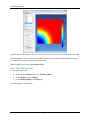
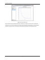
403 Poyntz Avenue, Suite B
Manhattan, KS 66502
USA
+1.785.770.8511
www.thunderheadeng.com
PetraSim Examples:
Five-Spot Geothermal Injection and
Production using Polygonal Cells and
Wells
2010
Table of Contents
Five-Spot Geothermal Injection and Production using Polygonal Cells and Wells ......................... 1
Add Wells..................................................................................................................................... 1
Create Mesh ................................................................................................................................ 1
Edit Well Flow Rates .................................................................................................................... 1
Save and Run ............................................................................................................................... 2
Save and Run with Well on Delivery Conditions ......................................................................... 4
View 3D Results ........................................................................................................................... 4
View Time History Plots............................................................................................................... 5
View Well Flow Time History Plots .............................................................................................. 6
ii
PetraSim Examples
Five-Spot Geothermal Injection and Production using Polygonal
Cells and Wells
We will repeat the previous example, but this time using a different mesh and wells to define the
injection and production. Open the Five-Spot Geothermal Production and Injection model and save it to
a new folder. This will preserve all the parameters not related to the mesh that we already defined in
the previous model.
Add Wells
To add wells:
1. On the Model menu, click Add Well…
2. In the Name box, type Inject
3. In the Ordered Well Coordinates table, type these values:
X
0.0
0.0
Y
0.0
0.0
Z
310.0
0.0
4. Click OK to create the well
5. Repeat this for the production well. Use the name Produce and the following coordinates:
X
500.0
500.0
Y
500.0
500.0
Z
310.0
0.0
Create Mesh
To create a polygonal (Voronoi) mesh:
1. On the Model menu, click Create Mesh
2. For Mesh Type, select Polygonal
3. Click OK to create the mesh
Your mesh should be refined near the wells, Figure
1. When a new mesh is created, the previous cellspecific properties, names and sources/sink data,
are erased.
Edit Well Flow Rates
Figure 1: Polygonal (Voronoi) mesh showing
refinement near wells
To define the injection rate:
1.
2.
3.
4.
In the Tree View, right-click on the Inject well and click Properties…
On the Flow tab, in the Injection section, select the Water/Steam check box
In the Rate box, type 7.5
In the Enthalpy box, type 50000 (corresponding to about 6 °C)
1
PetraSim Examples
5. Click the Print Options tab
6. Click to select the Print Time Dependent Flow and Generation Data check box
7. Click OK to save changes and close the dialog
To define the production rate:
1.
2.
3.
4.
5.
6.
In the Tree View, right-click on the Produce well and click Properties…
On the Flow tab, in the Production section, select the Mass Out check box
In the Rate box, type 7.5
Click the Print Options tab
Click to select the Print Time Dependent Flow and Generation Data check box
Click OK to save changes and close the dialog
Save and Run
The input is complete and you can run the simulation. Save your model and run the simulation:
1. On the Analysis menu, click Run TOUGH2
The solution will start and then Halt Prematurely. Click OK to
close the Error dialog.
In the Running TOUGH2 dialog, click on the Graph tab. This
display will show how the time step increased and then became small before halting. Next click on the
Log tab. This displays the error messages from the TOUGH2 output file. The critical message that will
cause convergence failure is EOS CANNOT FIND PARAMETERS AT ELEMENT * 3*. Use the Find function
and it will show that cell 3 is the cell that contains the production well.
So, in the previous example we were able to run with injection and production, but in this example the
solution failed. This provides a good example of the critical importance of physically meaningful
2
PetraSim Examples
boundary conditions in TOUGH2 . Specifying a constant production rate is not a realistic boundary
condition. In a real well, we cannot specify any desired production rate. In a real well, the production
rate depends on the fluid conditions and material properties of the reservoir and the geometry and
conditions of the production well. By specifying a fixed production rate, we have attempted to remove
mass at a higher rate than physically possible. As shown below, the pressure in the production cell goes
to zero and the equation of state is no longer valid.
The reason the pressure goes to zero is that the production cell size in the polygonal model is smaller
than in the uniform rectangular grid. We are trying to remove the same total flow rate from a smaller
cell. Since the flow area to the well is smaller, this requires a greater pressure drop into the cell,
lowering the pressure in the production cell until an unphysical state is reached in the model.
A better approximation of a real well can be made using the Productivity Index (see p.64 of the TOUGH2
user manual). Using the Productivity Index, the flow into the well is proportional to the pressure
difference between the well and containing cell.
To define the production well using the Productivity Index:
1.
2.
3.
4.
5.
6.
7.
8.
9.
10.
In the Tree View, right-click on the Produce well and click Properties…
Click on the Flow tab
In the Production section, click to clear the Mass Out check box
In the Production section, click to select the Well on Deliv check box
In the Productivity Index box, type 2.0E-12 (based on calculation described in the TOUGH2 User
Manual)
In the Pressure box, type 8.6E6 (the initial pressure in the model)
For Gradient, select Well Model
Click the Print Options tab
Click to select the Print Time Dependent Flow and Generation Data check box
Click OK to save changes and close the dialog
3
PetraSim Examples
Save and Run with Well on Delivery Conditions
The input is complete and you can run the simulation. Save your model and run the simulation:
1. On the Analysis menu, click Run TOUGH2
The Simulation Complete dialog will notify you when the end time has been reached. Click OK to dismiss
the notification and click Close to exit the Running TOUGH2 dialog.
View 3D Results
To open the 3D Results dialog:
1. On the Results menu, click 3D Results
By default, the display will show isosurfaces corresponding to pressure for the first output step.
To show temperature isosurfaces for the last time step:
1. In the Scalar list, click T
2. In the Time(s) list, click the last entry (t = 1.15183E9)
To show scalar data on a slice plane:
1.
2.
3.
4.
Click Slice Planes...
In the Axis list, click Z
In the Coord box, type 305
Click Close
To remove isosurfaces and show only slice data:
1. Click to clear the Show Isosurfaces check box
The resulting visualization is shown below:
4
PetraSim Examples
Figure 2: Temperature contours at end of solution for analysis using Productivity Index and Voronoi cells
Comparing Figure 2 to the previous results shows that there is not a pressure and temperature drop at
the production well when using the Productivity Index.
When finished, you can close the 3D Results dialog.
View Time History Plots
To view time history plots:
1. On the PetraSim Results menu, click Cell History Plots...
2. In the Variable list, click T (deg C)
3. In the Cell Name (Id#) list, click Inject (1)
The resulting plot is shown below.
5
PetraSim Examples
Figure 3: Temperature history of injection cell using polygonal mesh
Comparing Figure 3 with the previous example, shows again the effect of the small cell near the
injection well in the polygonal mesh. Because the cell that contains the injection well has a small volume
in the polygonal mesh, it cools much more rapidly than the larger cell in the rectangular mesh.
When finished, you can close the Cell History dialog.
View Well Flow Time History Plots
The total flow from the well can be plotted by:
1.
2.
3.
4.
5.
6.
7.
On the PetraSim Results menu, click Well Plots...
In the Variable list, click Flow Rate (kg/s)
In the Well Name list, click Produce (1)
On the View menu, click Range.
Click to clear Auto Range
In the X-Max box type 5.0E6
Click OK
The resulting plot is shown below.
6
PetraSim Examples
Figure 4: Flow at output well
Figure 4 shows how the production flow rate is initially zero, and then increases until it matches the
injection flow. The initial two-phase state of the model that provides compressibility, so that although
injection is constant, there is a time delay as the production increases to the steady state value.
7