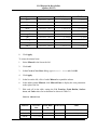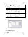
1
403 Poyntz Avenue, Suite B
Manhattan, KS 66502-6081
1.785.770.8511
www.thunderheadeng.com
PetraSim Example Manual
September 2008
TOUGHREACT Example Guide
Table of Contents
1. Overview .......................................................................................................................... 1
Using TOUGHREACT ................................................................................................. 1
Input Files ..................................................................................................................... 1
Thermodynamic Database ............................................................................................ 1
2. Aqueous Transport with Adsorption and Decay (EOS9) ............................................ 3
Description .................................................................................................................... 3
Specify the Equation of State (EOS) ............................................................................ 3
Create the Model Boundary .......................................................................................... 3
Create the Grid .............................................................................................................. 4
Global Properties .......................................................................................................... 5
Simulation Name .......................................................................................................... 5
EOS Data ...................................................................................................................... 5
Material Properties ........................................................................................................ 6
Material Data ................................................................................................................ 6
Relative Permeability .................................................................................................... 6
Capillary Pressure ......................................................................................................... 6
Initial Conditions .......................................................................................................... 7
Define Boundary Condtions ......................................................................................... 7
Water Source ................................................................................................................. 7
Production ..................................................................................................................... 8
Print Center Cell Data ................................................................................................... 8
Solution Controls .......................................................................................................... 9
Times ............................................................................................................................. 9
Weighting ...................................................................................................................... 9
Convergence ................................................................................................................. 9
Output Controls ........................................................................................................... 10
TOUGHREACT Solution Parameters ........................................................................ 11
TOUGHREACT Output Options ................................................................................ 11
TOUGHREACT Chemical Components .................................................................... 11
TOUGHREACT Zone Data ........................................................................................ 13
Associate Zones with Grid .......................................................................................... 15
Save and Run .............................................................................................................. 16
View 3D Results ......................................................................................................... 16
View Cell History Plots .............................................................................................. 17
3. CO2 Disposal in Deep Saline Aquifers (ECO2) ......................................................... 19
Description .................................................................................................................. 19
Specify the Equation of State (EOS) .......................................................................... 19
Global Properties ........................................................................................................ 19
Material Properties ...................................................................................................... 20
Material Data .............................................................................................................. 20
Relative Permeability .................................................................................................. 20
Capillary Pressure ....................................................................................................... 20
Miscellaneous ............................................................................................................. 21
Initial Conditions ........................................................................................................ 21
iv
TOUGHREACT Example
Guide
TOUGHREACT Solution Parameters ........................................................................ 22
TOUGHREACT Output Parameters ........................................................................... 22
TOUGHREACT Chemical Components .................................................................... 23
Primary Species .......................................................................................................... 23
Aqueous Complexes ................................................................................................... 24
Minerals ...................................................................................................................... 24
Gaseous Species .......................................................................................................... 28
TOUGHREACT Zone Data ........................................................................................ 28
Saving the Geochemical Data File as a Starting Point for a New Analysis ............... 31
Create the Model Boundary ........................................................................................ 31
Create the Grid ............................................................................................................ 32
Define Boundary Condtions ....................................................................................... 33
Solution Controls ........................................................................................................ 34
Times ........................................................................................................................... 34
Solver .......................................................................................................................... 35
Output Controls ........................................................................................................... 35
Associate Zones with Grid .......................................................................................... 35
Save and Run .............................................................................................................. 36
View Results ............................................................................................................... 37
The Continuation Run (Restart) .................................................................................. 38
Add Restart Data ......................................................................................................... 39
Set a New End Time ................................................................................................... 39
Start the Continuation Run ......................................................................................... 39
View Results ............................................................................................................... 39
References .......................................................................................................................... 41
v
List of Figures
2.1. Aqueous Transport with Adsorption and Decay Model (after [Xu, Sonnenthal, Spycher,
and Pruess, 2004]) ................................................................................................................. 3
2.2. The Create Grid dialog. The values shown will create a regular 60x1x1 grid .............. 5
2.3. Solution Controls - Convergence ................................................................................. 10
2.4. Primary Species ........................................................................................................... 12
2.5. 3D Results .................................................................................................................... 17
2.6. Cell History .................................................................................................................. 18
3.1. SAND Material Data .................................................................................................... 21
3.2. Primary Species ........................................................................................................... 23
3.3. Mineral Zone Data ....................................................................................................... 30
3.4. CO2 Injection ............................................................................................................... 33
3.5. CO2 Injection ............................................................................................................... 34
3.6. Zones Associated with Grid ......................................................................................... 36
3.7. Preparing a Line Plot ................................................................................................... 37
3.8. Line Plot of CO2 Saturation (Sg) ................................................................................. 38
3.9. Preparing a Line Plot ................................................................................................... 39
3.10. Line Plot of Total CO2 Sequestered in Minerals (SMco2) ........................................ 40
vi
List of Tables
2.1. Model Boundary Dimensions ........................................................................................ 3
2.2. Water Zone Data .......................................................................................................... 14
2.3. Water Zone Data .......................................................................................................... 14
3.1. Dissolution and Precipitation Data for Minerals ......................................................... 26
3.2. Additional Mechanism Data for Minerals ................................................................... 27
3.3. Dissolution and Precipitation Data for pyrite-2 ........................................................... 27
3.4. Additional Mechanism Data for pyrite-2 ..................................................................... 27
3.5. Water (Initial) Zone ..................................................................................................... 28
3.6. Mineral Zone ................................................................................................................ 29
3.7. Model Boundary Dimensions ...................................................................................... 31
vii
Chapter 1. Overview
Using TOUGHREACT
TOUGHREACT is an extension of the original TOUGH2 simulation that is available
as a simulator mode in PetraSim. The TOUGHREACT simulator supports a subset of
the TOUGH2 EOS modules. The supported EOS moduels are EOS1, EOS2, EOS3,
EOS9, and ECO2. You can perform a TOUGHREACT simulation by selecting the
TOUGHREACT simulator mode and one of the available EOS modules in the PetraSim Preferences dialog.
In PetraSim, options relating to TOUGHREACT are presented under the Tough React
menu item in the main window. These options allow you to configure the reactive
transport solver, simulation output, chemical zones, and other TOUGHREACT-specific parameters.
It is also possible to disable reactive transport during a TOUGHREACT simulation.
This will effectively revert the simulator to TOUGH2 mode. This option is available in
the Global Properties dialog, on the Analysis tab.
Input Files
A TOUGHREACT simulation requires four input files. These files are listed below:
•
flow.inp -- This is the standard TOUGH2 input file
•
solute.inp -- The chemical "geography" of the analysis
•
chemical.inp -- The chemical parameters
•
thermodb.txt -- The thermodynamic database
PetraSim creates each of these files into your simulation directory. However, the filenames cannot be changed. The naming scheme for the simulation output files follows a
similar pattern. To avoid overwriting previous simulation input and output data, you
must run each analysis in a separate directory.
Thermodynamic Database
A thermodynamic database listing the composition of many different species and minerals has been included with PetraSim. PetraSim will automatically load this database.
A valid database must be loaded prior to the inclusion of species or the definition of reactive zones. This is because the species used to build up the zones are loaded from the
thermodynamic database. If choose to use a custom databse, you must ensure that it is
loaded before configuring any species or zones. To load a custom thermodynamic
database:
1.
On the Tough React menu, click Thermodynamic Database...
1
Overview
2.
Select your custom thermodynamic database
3.
Click OK
2
Chapter 2. Aqueous Transport with Adsorption and Decay
(EOS9)
Description
This problem is the first example in the TOUGHREACT manual. It is a 1-D problem,
12 m in length, with a unit area, divided into 60 blocks of 0.2 m thickness, as shown in
Figure 2.1.
Figure 2.1. Aqueous Transport with Adsorption and Decay Model (after [Xu, Sonnenthal,
Spycher, and Pruess, 2004])
Specify the Equation of State (EOS)
To ensure that PetraSim uses TOUGHREACT and EOS9, you may need to edit your
PetraSim preferences. To edit preferences, you can use the Preferences dialog.
1.
On the File menu, click Preferences...
2.
In the Simulator Mode list, select TOUGHREACT
3.
In the Default Equation of State (EOS) list, select EOS9
4.
Click OK
Your preferences have now been updated, but you will need to create a new model or
restart PetraSim before they become active. If you already have a model open, it will
not be affected by the preference change.
On the File menu, click New.
Create the Model Boundary
To create the boundary for this model, use the Define Model Boundary dialog. The
boundary parameters for this model are shown in Table 2.1.
Table 2.1. Model Boundary Dimensions
3
Aqueous Transport with Adsorption and Decay (EOS9)
Axis
x
y
z
Min (m)
0.0
0.0
0.0
Max (m)
12.0
1.0
1.0
To create the model boundary:
1.
On the Model menu, click Define Boundary...
2.
Enter the values from Table 2.1
3.
Click OK to create the model boundary
Create the Grid
To create the gridas shown in Figure 2.2:
1.
On the Model menu, click Create Grid...
2.
In the Division Method box, select Regular
3.
In the X Cells box, type 60
4.
In the Y Cells box, type 1
5.
In the Z Cells box, type 1
6.
Click OK to create the grid
4
Aqueous Transport with Adsorption and Decay (EOS9)
Figure 2.2. The Create Grid dialog. The values shown will create a regular 60x1x1 grid
Global Properties
Global properties are properties that apply to the entire model. In this example, the
only thing we will change is the analysis name. To edit global properties, you can use
the Global Properties dialog.
On the Properties menu, click Global Properties...
Simulation Name
1.
In the Global Properties dialog, click the Analysis tab
2.
In the Name box, type TOUGHREACT Example 1
EOS Data
The EOS (Equation of State) tab displays options for EOS9.
1.
In the Global Properties dialog, click the EOS tab
2.
In the Reference Pressure (Pa) box, type 1.0E5
5
Aqueous Transport with Adsorption and Decay (EOS9)
3.
In the Reference Temperature (C) box, type 4.0
Click OK to close the Global Properties dialog.
Material Properties
To specify the material properties, you use the Material Data dialog. This example requires one material.
To open the Material Data dialog: on the Properties menu, click Materials...
Material Data
1.
In the materials list, select ROCK1
2.
In all three Permeability boxes (X, Y, and Z), type 6.51E-12
3.
In the Wet Heat Conductivity box, type 0.0
4.
In the Specific Heat box, type 952.9
5.
Click Apply to save the changes
In addition to the physical rock parameters, we also need to specify the relative permeability and capillary pressure functions for this material. These options can be found
in the Additional Material Data dialog. To open this dialog, click the Additional
Material Data... button.
Relative Permeability
To specify the relative permeability function:
1.
Click the Relative Perm tab
2.
In the Relative Permeability list, select Linear Functions
3.
In the Slmin box, type 0.333
4.
In the Slmax box, type 1.0
5.
In the Sgmin box, type -0.1
6.
In the Sgmax box, type 0.0
Capillary Pressure
To specify the capillary pressure function:
1.
Click the Capillary Press tab
6
Aqueous Transport with Adsorption and Decay (EOS9)
2.
In the Capillary Pressure list, select Linear Function
3.
In the CPmax box, type 9.7902E3
4.
In the A box, type 0.333
5.
In the B box, type 1.0
Click OK to exit the Additional Material Data dialog.
Click OK again to save your settings and exit the Material Data dialog.
Initial Conditions
The initial state of each cell in the model must be defined. The Default Initial Conditions dialog is used to define initial conditions that will be applied to the entire model.
You can also specify initial conditions by cell, by region, or by importing the results of
a previous analysis. For any analysis, the specific initial conditions will depend on several factors including EOS selection, simulator mode, and the initial state of the simulation.
Correct specification of initial conditions is essential for proper convergence and obtaining a correct result. In general, the initial conditions need to physically meaningful.
Often this requires an initial state analysis in which a model is run to obtain initial
equilibrium conditions before the analysis of interest (geothermal production, VOC
spill, etc.) is run.
To edit global initial conditions: on the Properties menu, click Initial Conditions...
To set the initial conditions:
1.
In the list, select Pressure
2.
In the Pressure box, type 1.001E5
Click OK to exit the Default Initial Conditions dialog.
Define Boundary Condtions
To edit cells, you can use the Grid Editor. In this case, we will use the Grid Editor to
define boundary conditions in the model.
To open the Grid Editor: on the Model menu, click Edit Grid.
Water Source
We will inject into the cell on the left and produce from the cell on the right. Click on
the leftmost cell in the grid (cell #1). To edit the properties of this cell, on the Edit
menu, click Properties.
7
Aqueous Transport with Adsorption and Decay (EOS9)
Click the Properties tab. Then, in the Cell Name box, type Input.
Click the Sources/Sinks tab. To define the source:
1.
Under Injection, select Water
2.
In the Rate box, type 1.16E-4
3.
Because EOS9 is an isothermal analysis, the enthalpy value need not be set
Next, click the Print Options tab. Select Print Cell Time Dependent Flow and Generation (BC) Data. This will output data for this cell at every time step, which can
then be used to make detailed time history plots.
Click OK to close the Edit Cell Data dialog.
Similar steps are followed to define production in the model.
Production
We will produce from the cell on the right. Click on the rightmost cell in the grid (cell
#60). To edit the properties of this cell, on the Edit menu, click Properties.
Click the Properties tab. Then, in the Cell Name box, type Output.
Select the Sources/Sinks tab. To define the production:
1.
Under Production, select Mass Out
2.
In the Rate box, type 1.16E-4
Next, click the Print Options tab. Select Print Cell Time Dependent Flow and Generation (BC) Data.
Click OK to close the Edit Cell Data dialog.
Print Center Cell Data
In the grid editor, we will also choose a cell in the center of the model for which time
history data will be printed. Right-click on a cell near the center (for example, cell #30)
to edit the cell properties.
Click the Properties tab. Then, in the Cell Name box, type Center
Unlike the Input and Output cells, do not set any boundary condition data for the Center cell
8
Aqueous Transport with Adsorption and Decay (EOS9)
Click the Print Options tab. Select Print Cell Time Dependent Flow and Generation (BC) Data.
Click OK to close the Edit Cell Data dialog.
On the File menu, click Close to exit the grid editor.
Solution Controls
We will now define the solution options. Options relating the time step and other solution controls can be found in the Solution Controls dialog.
To open the Solution Controls dialog: on the Analysis menu, click Solution Controls...
Times
1.
In the Solution Controls dialog, click the Times tab
2.
In the End Time box, type 8.64E6
3.
In the Time Step box, type 10.0
4.
In the Max Num Time Steps list, type 1000
5.
In the Max Time Step list, select User Defined
6.
In the Max Time Step box, type 8.64E3
For consistency with the example problem, we will now change some of the default
values. In most cases, these values would not be changed.
Weighting
1.
In the Solution Controls dialog, click the Weighting tab
2.
As the Density at Interface option, select Average of Adjacent Elements
Convergence
1.
In the Solution Controls dialog, click the Convergence tab
2.
In the Relative Error Criterion box, type 1.0E-6
9
Aqueous Transport with Adsorption and Decay (EOS9)
Figure 2.3. Solution Controls - Convergence
Click OK to exit the Solution Controls dialog.
Output Controls
By default, the simulation will print output every 100 time steps. We can change the
resolution of the output in the Output Controls dialog.
1.
On the Analysis menu, click Output Controls...
2.
In the Print and Plot Every # Steps box, type 500
3.
In the Additional Output Datagroup, select Fluxes and Velocities, Primary
Variables, and Additional T2React Variables
In addition to printing output every 500 steps, we can also specify times for which we
want to view data in the Additional Print Times dialog.
To specify additional times for output:
1.
On the Output Controls dialog, click the Edit button to open the Additional
Print Times dialog
2.
In the Times table, type 4.32E6 and 8.64E6
10
Aqueous Transport with Adsorption and Decay (EOS9)
3.
Click OK to exit the Additional Print Times dialog.
Click OK to exit the Output Controls dialog.
TOUGHREACT Solution Parameters
We will now set the TOUGHREACT parameters. In this example, we are doing this
last, since the entire model will lie in the same zone. However, if we wanted to define
different zones in the model, we would specify the TOUGHREACT parameters first.
TOUGHREACT solution parameters can be entered on the Solution Parameters dialog. To open the Solution Parameters dialog: on the Tough React menu, click Solution Parameters....
Select Advanced from the list on the left, to display the Advanced Options pane. Under the Advanced Options, select Print Porosity, Permeability, Capillary Pressure
Changes.
Next, select Times and Convergence from the list on the left, to open the Time Stepping and Convergence Options pane.
In the Max Iterations to Solve Geochemical System box, type 300.
In the Relative Sorption Concentration Tolerance box, type 1.0E-6.
Click OK to exit the Solver Parameters dialog.
TOUGHREACT Output Options
TOUGHREACT output options can be changed on the Output Options dialog.
1.
On the Tough React menu, click Output Options....
2.
In the Grid Block Output Frequency(s) box, type 40.
3.
For Aqueous Concentration Output, select Write Total Aqueous Component
Concentrations.
4.
For Aqueous Concentration Units, select mol/L Liquid.
5.
For Mineral Abundance Units, select Change in Volume Fraction.
Click OK to exit the Output Options dialog.
TOUGHREACT Chemical Components
TOUGHREACT chemical components can be specified in the Chemical Components
dialog. To open the Chemical Components dialog: on the Tough React menu, select
Chemical Components....
11
Aqueous Transport with Adsorption and Decay (EOS9)
To define the primary species:
1.
In the list on the left of the Chemical Components dialog, select Primary Species
2.
In the Thermodynamic Database list in the middle of the dialog, select h+, h2o,
na+, skdd1, skdd2, and skdd3
3.
Click the --> button to move the selected species into the Current Simulation list
on the right, as shown in Figure 2.4.
Figure 2.4. Primary Species
4.
Click Apply to add the selected species to the analysis
The parameters specific to each type can be viewed and changed by clicking on that
type in the subtree under Primary Species in the list on the left.
To edit parameters for na+ :
1.
Select na+ in the list under Primary Species.
2.
In the pane on the right, select Output Concentration History at Selected Cells.
This will output additional data for cells that have previously been identified for
printing time history data.
To edit parameters for skdd1 :
1.
Select skdd1 in the list
12
Aqueous Transport with Adsorption and Decay (EOS9)
2.
In the pane on the right, select Output Concentration History at Selected Cells
3.
Select Enable Kd and Decay.
4.
In the Decay Constant box, type 0.0
To edit parameters for skdd2 :
1.
Select skdd2 in the list
2.
In the pane on the right, select Output Concentration History at Selected Cells
3.
Select Enable Kd and Decay.
4.
In the Decay Constant box, type 4.0113E-7
To edit parameters for skdd3 :
1.
Select skdd3 in the list
2.
In the pane on the right, select Output Concentration History at Selected Cells
3.
Select Enable Kd and Decay.
4.
In the Decay Constant box, type 4.0113E-7
Click OK to exit the Chemical Components dialog.
TOUGHREACT Zone Data
The next task is to create the zone data, which can be done in the Geochemical Zones
dialog. To open the Geochemical Zones dialog: on the Tough React menu, click
Zone Data.... Initially, there will not be any zones in the mdoel.
To create the initial water zone:
1.
Select Water (Initial) in the list on the left
2.
Click Add
3.
In the Create a New Zone dialog, type Water Zone and click OK
4.
Click Apply
5.
In the list on the left, click + beside Water (Initial) to expand the subtree.
6.
In the subtree under Water (Initial), click Water Zone to display the zone parameters to the right of the list.
13
Aqueous Transport with Adsorption and Decay (EOS9)
7.
Enter the data that is shown in Table 2.2
Table 2.2. Water Zone Data
Species
h+
h20
na+
skdd1
skdd2
skdd3
Constraint
Amount (mol)
Amount (mol)
Amount (mol)
Amount (mol)
Amount (mol)
Amount (mol)
CGUESS
CTOT
1.0e-7
1.0
1.0e-10
1.0e-10
1.0e-10
1.0e-10
1.0e-7
1.0
1.0e-10
1.0e-10
1.0e-10
1.0e-10
To create the boundary water zone:
1.
Select Water (Boundary) in the list on the left
2.
Click Add
3.
In the Create a New Zone dialog, type Water Boundary Zone and click
OK
4.
Click Apply
5.
In the list on the left, click + beside Water (Boundary) to expand the subtree.
6.
In the subtree under Water (Boundary), click Water Boundary Zone to display
the zone parameters to the right of the list
7.
Enter the data that is shown in Table 2.3
Table 2.3. Water Zone Data
Species
h+
h20
na+
skdd1
skdd2
skdd3
Constraint
Amount (mol)
Amount (mol)
Amount (mol)
Amount (mol)
Amount (mol)
Amount (mol)
To create the permeability porosity zone:
14
CGUESS
CTOT
1.0e-7
1.0
1.0e-4
1.0e-4
1.0e-4
1.0e-4
1.0e-7
1.0
1.0e-4
1.0e-4
1.0e-4
1.0e-4
Aqueous Transport with Adsorption and Decay (EOS9)
1.
Select Permeability Porosity in the list on the left
2.
Click Add
3.
In the Create a New Zone dialog, type Perm/Por Zone and click OK
4.
Click Apply
5.
In the list on the left, click + beside Permeability Porosity to expand the subtree.
6.
In the subtree under Permeability Porosity, click Perm/Por Zone to display the
zone parameters to the right of the list
7.
Select Modified Cubic Law
To create the linear Kd zone:
1.
Select Linear Kd in the list on the left
2.
Click Add
3.
In the Create a New Zone dialog, type Linear Kd Zone and click OK
4.
Click Apply
5.
In the list on the left, click + beside Linear Kd to expand the subtree.
6.
In the subtree under Linear Kd, click Linear Kd Zone to display the zone parameters to the right of the list
7.
For skdd1 and skdd3, in the Density box, type 2.6 and in the Kd box, type
4.2735E-2
Click OK to exit the Geochemical Zones dialog.
Associate Zones with Grid
The last task is to associate zones with the grid. This can be done in two ways, either
by region or for individual cells in the Grid Editor. Initially the model is one region,
but it can be subdivided into more regions by using internal boundaries. This can be
useful, since it is also possible to assign material data and initial conditions by region.
In this case, the model will remain a single region.
Click on the model to select it in entirety. You can better see the model selection by
unselecting Grid in the View menu.
After the model has been selected:
1.
Under the Model menu, click Edit Selection to open the Edit Region Data dia15
Aqueous Transport with Adsorption and Decay (EOS9)
log
2.
Click the Chemical Zones tab
3.
Select Specify Zones by Region
4.
From the Initial Water Zone, Boundary Water Zone, Permeability/Porosity
Zone, and Linear Kd Zone lists, select the respective zones that have previously
been created.
Click OK to exit the Edit Region Data dialog.
Save and Run
The input is complete and you can run the simulation. If you haven't already, you may
want to save your model in a directory specifically intended for the simulation results.
For example:
1.
On the File menu, click Save As...
2.
In
the
File
Name
box,
C:\t2react_example1\t2react_example1.sim
3.
Click Save
type
To run the simulation: on the Analysis menu, click Run T2REACT
View 3D Results
To view the 3D results for a simulation: on the Results menu, click 3D Results. The
data for the current simulation will be automatically loaded and displayed.
Because this is a 1-D model, the isosurfaces do not display the data well. To turn off
the isosurfaces: on the View menu, click Show Isosurfaces
We will instead define a slice plane through the model to better display the output data.
To create a slice plane:
1.
On the Results menu, click Slice Planes
2.
In the topmost Axis list, select Z
3.
In the topmost Coord box, type 0.5
4.
Click Close to close the Slice Planes dialog
To view 3D results, as shown in Figure 2.5:
1.
In the Time(s) list, select 0.13689
16
Aqueous Transport with Adsorption and Decay (EOS9)
2.
In the Scalar list, select na+
3.
Use the mouse to rotate the model to a good viewing perspective
Figure 2.5. 3D Results
On the File menu, click Close to close the 3D Results dialog.
View Cell History Plots
You can view time history plots with the Cell History dialog. On the Results menu,
click Cell History Plots.....
The Cell History dialog will be displayed. In this window, you can display time history data using a plotting parameter and a list of cells. For example, to view the isosurfaces for the Center cell, as shown in Figure 2.6:
1.
In the Variable list, select na+
2.
In the Cell Name (Id#) list, select Center
17
Aqueous Transport with Adsorption and Decay (EOS9)
Figure 2.6. Cell History
In the File menu, click Close to close the Cell History window.
18
Chapter 3. CO2 Disposal in Deep Saline Aquifers (ECO2)
Description
This problem is example five in the TOUGHREACT manual. It is a 1-D radial problem in which CO2 is injected into a well field 100 m in depth and extending with a
100,000 m radius. CO2 is injected at a rate of 90 kg/s, which is approximately equivalent to that generated by a 300 MW coal-fired power plant. The CO2 injection continues for 100 years. This problem demonstrates the restart feature to run for an additional
900 years with no additional CO2 injection.
Entering some parameters for the geochemical system in this example problem can be
time-intensive. To bypass entering the parameters for chemical components, please
open the file geochem_basic.sim after updating your EOS preferences (but before editing global properties). This file is available online via the PetraSim documentation page or on your PetraSim install CD.
Specify the Equation of State (EOS)
To ensure that PetraSim uses TOUGHREACT and ECO2, you may need to edit your
PetraSim preferences. To edit preferences, you can use the Preferences dialog.
1.
On the File menu, click Preferences...
2.
In the Simulator Mode list, select TOUGHREACT
3.
In the Default Equation of State (EOS) list, select ECO2N
4.
Click OK
Your preferences have now been updated, but you will need to create a new model or
restart PetraSim before they become active. If you already have a model open, it will
not be affected by the preference change.
On the File menu, click New.
Global Properties
We will first define all material and chemical properties, beginning by defining analysis options related to the equation of state (ECO2).
To edit global properties: on the Properties menu, click Global Properties...
1.
Click the Analysis tab
2.
In the Name box, type CO2 Injection
3.
Click the EOS tab
19
CO2 Disposal in Deep Saline
Aquifers (ECO2)
4.
Select Isothermal
5.
In the Brine Density in CO2 box, click Independent.
Click OK to exit the Global Properties dialog.
Material Properties
We next define the material properties. Since this problem uses only one material, we
will simply modify the default material.
To edit material properties: on the Properties menu, click Materials...
Material Data
1.
In the Name box, type SAND
2.
In the Porosity box, type 0.3
3.
In the three (x, y, and z) permeability boxes, type 1.0E-13
4.
In the Wet Heat Conductivity box, type 2.51
5.
In the Specific Heat box, type 920
Relative Permeability
1.
Click Relative Perm... to open the Additional Material Data dialog
2.
Click the Relative Perm tab
3.
In the Relative Permeability list, select van Genuchten-Mualem Model
4.
In the RP(1) box, type 0.457
5.
In the Slr box, type 0.3
6.
In the Sls box, type 1.0
7.
In the Sgr box, type 0.05
Capillary Pressure
1.
Click the Capillary Press tab
2.
In the Capillary Pressure list, select van Genuchten Function
3.
In the CP(1) box, type 0.457
20
CO2 Disposal in Deep Saline
Aquifers (ECO2)
4.
In the Slr box, type 0.0
5.
In the 1/P0 box, type 5.1E-5
6.
In the Pmax box, type 1.0E7
7.
In the Sls box, type 0.999
Miscellaneous
1.
Click the Misc tab
2.
In the Pore Compressibility box, type 4.5E-10
Click OK to exit the Additional Material Data dialog.
Figure 3.1. SAND Material Data
Click OK again to exit the Material Data dialog.
Initial Conditions
To open the Default Initial Conditions dialog: on the Properties menu, click Initial
Conditions...
1.
In the ECO2 list, select Two Fluid Phases (P, Xsm, Sg, T)
2.
In the Pressure box, type 2.0E7
3.
In the Temperature box, type 75.0
21
CO2 Disposal in Deep Saline
Aquifers (ECO2)
4.
In the Gas Saturation box, type 0.0
5.
In the Salt Mass Fraction box, type 0.06
Click OK to exit the Default Initial Conditions dialog.
TOUGHREACT Solution Parameters
TOUGHREACT solution parameters can be set in the Solver Parameters dialog. To
open the Solver Parameters dialog: on the Tough React menu, click Solution Parameters...
Click Standard
1.
Click to select Enable Gaseous Species Transport
Click Advanced
1.
Click to de-select Ignore Mineral Dissolution/Precipitation Effects on Flow
2.
Under Effect of CO2 and H2O Reactions on Flow, click to select CO2 and
H2O
Click Validation
1.
In the Max Stochiometric Ionic Strength box, type 6.0
Click Times and Convergence
1.
In the Relative Transport Concentration Tolerance, type 1.0E-6
2.
In the Relative Sorbtion Concentration Tolerance, type 1.0E-6
Click Diffusion Coefficients
1.
In the Aqueous Species Diffusion Coefficient box, type 1.0E-9
2.
In the Gaseous Species Diffusion Coefficient box, type 1.1E-5
Click OK to exit the Solver Parameters dialog.
TOUGHREACT Output Parameters
TOUGHREACT output parameters can be set in the Output Options dialog. To open
the Output Options dialog: on the Tough React menu, click Output Options...
1.
Under Aqueous Concentration Output, select Write Total Aqueous Component Concentrations
22
CO2 Disposal in Deep Saline
Aquifers (ECO2)
2.
Under Mineral Abundance Units, select Change in Volume Fraction
Click OK to exit the Output Options dialog.
TOUGHREACT Chemical Components
TOUGHREACT chemical components can be specified in the Chemical Components
dialog. To open the Chemical Components dialog: on the Tough React menu, select
Chemical Components....
The thermodynamic database contains the master list of chemical components. To use
a species (of any type), we first add the species to the simulation, then configure the
simulation-specific properties for that species.
Primary Species
To define the primary species:
1.
In the list on the left of the Chemical Components dialog, select Primary Species
2.
In the Thermodynamic Database list in the middle of the dialog, select alo2-,
ca+2, cl-, fe+2, h+, h2o, hco3-, k+, mg+2, na+, o2(aq), sio2(aq), and so4-2.
3.
Click the --> button to move the selected species into the Current Simulation list
on the right
4.
Click Apply to add the selected species to the analysis
Figure 3.2. Primary Species
23
CO2 Disposal in Deep Saline
Aquifers (ECO2)
The parameters specific to each type can be viewed and changed by clicking on that
type in the subtree under Primary Species in the list on the left. For this simulation,
there is no need to edit any additional parameters.
Aqueous Complexes
A similar process is used to define the aqueous complexes:
1.
In the list on the left of the Chemical Components dialog, select Aq. Complexes
2.
For Specify Secondary Species, select Select Species Individually
3.
In the Thermodynamic Database list in the middle of the dialog, select acetic~acid(aq), al(oh)2+, al(oh)3(aq), al+3, aloh+2, cacl+, cacl2(aq), caco3(aq),
cahco3+, caoh+, caso4(aq), ch4(aq), co2(aq), co3-2, fe+3, fecl+, fecl4-2,
feco3(aq), fehco3+, h2(aq), h2s(aq), h3sio4-, halo2(aq), hs-, hso3-, kcl(aq),
kso4-, mgcl+, mghco3+, mgso4(aq), naalo2(aq), nacl(aq), naco3-,
nahco3(aq),nahsio3(aq), naoh(aq), naso4-, oh-, and so2(aq)
4.
Click the --> button to move the selected species into the Current Simulation list
on the right
5.
Click Apply to add the selected species to the analysis
Minerals
A similar process is used to define the minerals:
1.
In the list on the left of the Chemical Components dialog, select Minerals
2.
In the Thermodynamic Database in the middle of the dialog, select albite~low,
ankerite-2, calcite, chlorite, dawsonite, dolomite-2, hematite, illite, k-feldspar,
kaolinite, magnesite, oligoclase, pyrite-2, quartz, siderite-2, smectite-ca, and
smectite-na
3.
Click the --> button to move the selected species into the Current Simulation list
on the right
4.
Click Apply to add the selected minerals to the analysis
The parameters specific to each mineral can be viewed and changed by clicking on that
type in the subtree under Minerals in the list on the left.
Each mineral has unique dissolution, precipitation, and additional mechanisms properties. The values for each of these properties for each mineral are shown in Table 3.1,
and Table 3.2. Pyrite is a bit different than the other minerals and its properties are
shown in Table 3.3 and Table 3.4. This section will demonstrate how to specify the
properties for albite~low, then you should be able to enter the remaining mineral
properties by following the same pattern and referring to the tables.
24
CO2 Disposal in Deep Saline
Aquifers (ECO2)
Please note, if table entries are blank, then those parameters should not be set. The
mineral calcite is considered to be at equilibrium and no parameters for dissolution, precipitation, or additional mechanisms should be specified. The mineral
quartz has no additional mechanisms. Several minerals have only 1 additional mechanism.
Select albite~low in the list under Minerals.
To edit dissolution rate parameters for albite~low:
1.
Under Specify Kinetic Constraints, click to select Dissolution.
2.
Click Edit... This will open the Edit dissolution Rate Parameters dialog.
3.
In the Activation Energy - EA box, type 69.8 (from Table 3.1).
4.
In the Rate Constant k25 box, type 2.7542e-13 (from Table 3.1).
5.
Click OK to save changes and exit the Edit Dissolution Rate Parameters dialog.
To edit precipitation rate parameters for albite~low:
1.
Under Specify Kinetic Constraints, click to select Precipitation.
2.
Click Edit... This will open the Edit Precipitation Rate Parameters dialog.
3.
On the Options tab, in the Initial Volume Fraction box, type 1.0e-6.
4.
Click the Energy tab.
5.
In the Activation Energy - EA box, type 69.8 (from Table 3.1).
6.
In the Rate Constant k25 box, type 2.7542e-13 (from Table 3.1).
7.
Click OK to save changes and exit the Edit Dissolution Rate Parameters dialog.
To add additional mechanisms for albite~low:
1.
Under Rate Constant Dependence on pH, click to select Specify Additional
Mechanisms.
2.
Click Edit... This will open the Edit Additional Mechanisms dialog.
3.
Click New. This will create Mechanism (1).
4.
In the Weighting Factor box, type 6.9183e-11 (from Table 3.2)
5.
In the Activation Energy box, type 65.0 (from Table 3.2)
6.
In the table, in the Species list, select h+ (from Table 3.2).
25
CO2 Disposal in Deep Saline
Aquifers (ECO2)
7.
In the table, in the Exponent box, type 0.457 (from Table 3.2).
8.
Click New. This will create Mechanism (2).
9.
In the Weighting Factor box, type 2.5119e-16 (from Table 3.2)
10. In the Activation Energy box, type 71.0 (from Table 3.2)
11. In the table, in the Species list, select h+ (from Table 3.2).
12. In the table, in the Exponent box, type -0.572 (from Table 3.2).
13. Click OK to save changes and exit the Edit Dissolution Rate Parameters dialog.
All other selected minerals should be edited in this fashion, using the values shown in
Table 3.1 and Table 3.2. Data for pyrite-2 can be found in Table 3.3 and Table 3.4.
Empty table cells indicate that the existing data is already correct and that new data
need not be entered (i.e. if there is no entry for a particular option, do not enable that
option).
Table 3.1. Dissolution and Precipitation Data for Minerals
Mineral
albite~low
ankerite-2
calcite
chlorite
dawsonite
dolomite-2
hematite
illite
k-feldspar
kaolinite
magnesite
oligoclase
quartz
siderite-2
smectite-ca
smectite-na
Activation
Rate ConEnergy
stant k25
69.8 2.754E-13
62.76 1.260E-09
88
62.76
52.2
66.2
35
38
22.2
23.5
69.8
87.7
62.76
35
35
3.020E-13
1.260E-09
2.951E-08
2.514E-15
1.660E-13
3.890E-13
6.918E-14
4.571E-10
1.445E-12
1.023E-14
1.260E-09
1.660E-13
1.660E-13
26
CO2 Disposal in Deep Saline
Aquifers (ECO2)
Table 3.2. Additional Mechanism Data for Minerals
Mineral
albite~low
ankerite-2
calcite
chlorite
dawsonite
dolomite-2
hematite
illite
k-feldspar
kaolinite
magnesite
oligoclase
quartz
siderite-2
smectite-ca
smectite-na
Mechanism(1)
Mechanism(2)
Weighting
Activation n(H+) Expo- Weighting
Activation n(H+) ExpoFactor k25
Energy
nent
Factor k25
Energy
nent
6.918E-11
65.0
0.457 2.512E-16
71
-0.572
6.457E-04
36.1
0.500
7.762E-12
6.457E-04
6.457E-04
4.074E-10
1.047E-11
8.710E-11
4.898E-12
4.169E-7
2.138E-10
88.0
36.1
36.1
66.2
23.6
51.7
65.9
14.4
65.0
0.500
0.500
0.5
1.0
0.340 3.020E-17
0.500 6.310E-22
0.777 8.913E-18
1.0
0.457
6.457E-04
1.047E-11
1.047E-11
36.1
23.6
23.6
0.500
0.34 3.020E-17
0.340 3.020E-17
58.9
94.1
17.9
-0.400
-0.823
-0.472
58.9
58.9
-0.400
-0.400
Table 3.3. Dissolution and Precipitation Data for pyrite-2
Mineral
pyrite-2
Dissolution
Precipitation
Activation
Rate ConActivation
Rate ConEnergy
stant k25
Energy
stant k25
0.0
0.0
56.9
4.0e-11
Table 3.4. Additional Mechanism Data for pyrite-2
Mineral
pyrite-2
Mechanism(1)
Mechanism(2)
Weighting
Activation
Exponents
Weighting
Activation
Exponent
Factor
Energy (Ea)
Factor k25
Energy
3.02e-8
56.9
[h+, - 2.8184e-5
56.9 [o2(aq),
0.5]
0.5]
[fe+3,
0.5]
27
CO2 Disposal in Deep Saline
Aquifers (ECO2)
To save these changes: click Apply
Gaseous Species
1.
In the list on the left of the Chemical Components dialog, select Gaseous Species
2.
In the Thermodynamic Database list in the middle of the dialog, select co2(g),
3.
Click the --> button to move co2(g) into the Current Simulation list on the right
4.
Click Apply to add the selected species to the analysis
Click OK to exit the Chemical Components dialog.
TOUGHREACT Zone Data
Geochemical zones describe the initial chemical composition of the model. You can
define geochemical zones using the Geochemical Zones dialog. To open the Geochemical Zones dialog: on the Tough React menu, click Zone Data.... Initially, there
will not be any zones in the mdoel.
To create the water zone:
1.
Select Water (Initial) in the list on the left
2.
Click Add
3.
In the Create a New Zone dialog, type Water Zone and click OK
4.
Click Apply
5.
In the list on the left, click + beside Water (Initial) to expand the subtree
6.
In the subtree under Water (Initial), click Water Zone to display the zone parameters to the right of the list
7.
Edit each cell in the table, setting the Constraint, CGUESS, and CTOT values
for each species as shown in Table 3.5.
Table 3.5. Water (Initial) Zone
Species
alo2ca+2
cl-
Constraint
Amount (mol)
Amount (mol)
Amount (mol)
28
CGUESS
1.078e-8
4.479e-3
0.9109
CTOT
1.361e-8
4.737e-3
1.001
CO2 Disposal in Deep Saline
Aquifers (ECO2)
Species
fe+2
h+
h2o
hco3k+
mg+2
na+
o2(aq)
sio2(aq)
so4-2
8.
Constraint
Amount (mol)
Amount (mol)
Amount (mol)
Amount (mol)
Amount (mol)
Amount (mol)
Amount (mol)
Amount (mol)
Amount (mol)
Amount (mol)
CGUESS
2.615e-7
8.48e-8
1.0
1.841e-8
5.805e-3
2.348e-5
0.9006
2.763e-66
9.203e-4
1.443e-16
CTOT
3.022e-7
0.0432
1.0
4.562e-2
5.980e-3
2.669e-5
0.9905
-8.646e-2
1.034e-3
1.324e-9
Click Apply
To create the mineral zone:
1.
Select Mineral in the list on the left
2.
Click Add
3.
In the Create a New Zone dialog, type Mineral Zone and click OK
4.
Click Apply
5.
In the list on the left, click + beside Mineral to expand the subtree
6.
In the subtree under Mineral, click Mineral Zone to display the zone parameters
to the right of the list
7.
Edit each cell in the table, setting the Vol. Fraction, Grain Radius, Surface
Area, and Units values for each mineral as shown in Table 3.6.
Table 3.6. Mineral Zone
Mineral
albite~low
ankerite-2
calcite
Vol. Fraction
Grain Radi- Surface Area
us
0
0.001
9.8
0
0.001
9.8
0.01929
29
Units
cm^2/g mineral
cm^2/g mineral
CO2 Disposal in Deep Saline
Aquifers (ECO2)
Mineral
chlorite
dawsonite
dolomite-2
hematite
illite
k-feldspar
kaolinite
magnesite
oligoclase
pyrite-2
quartz
siderite-2
smectite-ca
smectite-na
8.
Vol. Frac- Grain Radi- Surface Area
tion
us
0.04556
0.001
9.8
0
0.001
9.8
0
0.001
9.8
0.00497
0.001
12.87
0.00954
0.001
151.63
0.08179
0.001
9.8
0.02015
0.001
151.6
0
0.001
9.8
0.19795
0.001
9.8
0
0.001
12.87
0.57888
0.001
9.8
0
0.001
9.8
0
0.001
151.63
0.03897
0.001
151.63
Click Apply
Figure 3.3. Mineral Zone Data
To create the permeability porosity zone:
1.
Select Permeability Porosity in the list on the left
2.
Click Add
30
Units
cm^2/g
cm^2/g
cm^2/g
cm^2/g
cm^2/g
cm^2/g
cm^2/g
cm^2/g
cm^2/g
cm^2/g
cm^2/g
cm^2/g
cm^2/g
cm^2/g
mineral
mineral
mineral
mineral
mineral
mineral
mineral
mineral
mineral
mineral
mineral
mineral
mineral
mineral
CO2 Disposal in Deep Saline
Aquifers (ECO2)
3.
In the Create a New Zone dialog, type Perm-Pore Zone and click OK
4.
Click Apply
5.
In the list on the left, click + beside Permeability Porosity to expand the subtree
6.
In the subtree under Permeability Porosity, click Perm-Pore Zone to display the
zone parameters to the right of the list
7.
For Permeability Law, select Cubic Law
8.
Click Apply
Click OK to exit the Geochemical Zones dialog.
Saving the Geochemical Data File as a Starting Point for a New
Analysis
All of the problem data that is not specific to a particular geometry and loading condition has now been defined. At this point, save the data by clicking Save... on the File
menu, and typing "geochemical data" as the file name. We can now open "geochemical data" and click Save As... on the File menu, giving the new name as
"eco2_example". Anytime you want to create a model that uses the same (or similar) geochemical data, you can open the "geochemical data" file and save it as a different file as a starting point for a different analysis. In this manner you can avoid repeating all the data input.
In continuing this example, model specific data will now be entered and simulated.
Create the Model Boundary
To create the boundary for this model, use the Define Model Boundary dialog. The
boundary parameters for this model are shown in Table 3.7.
Table 3.7. Model Boundary Dimensions
Axis
x
y
z
Min (m)
0.0
0.0
-100.0
Max (m)
100000.0
1.0
0.0
To create the model boundary:
31
CO2 Disposal in Deep Saline
Aquifers (ECO2)
1.
On the Model menu, click Define Boundary...
2.
Enter the values from Table 3.7
3.
Click OK to create the model boundary
Create the Grid
To create the grid:
1.
On the Model menu, click Create Grid...
2.
In the Division Method box, select Regular
3.
For Grid Type, select RZ Grid
4.
In the X Cells box, type 100
5.
In the X Factor box, type 1.1096251
6.
In the Z Cells box, type 1
7.
In the Z Factor box, type 1.0
8.
Click OK to create the grid
This 100 cell grid used here is different than the 130 cell meshmaker grid used in the
example problem writeup from the TOUGHREACT user's manual. The style of the
grid used in TOUGHREACT user's manual would require a logarithmic capability in
PetraSim's meshmaker grid creater that is currently not supported. The 100 cell logarithmic grid used in this example problem appears to be sufficient based on a sensitivity
analysis (Figure 3.4) of the Sg parameter after 100 years of simulation with different
grid sizes.
32
CO2 Disposal in Deep Saline
Aquifers (ECO2)
Figure 3.4. CO2 Injection
To use a 200 cell grid, change the value of the X Cells paramter to 200 and the value
of the X Factor parameter to 1.04950055. The running time of this simulation is
linear in the number of cells. It takes approximately 10 minutes to run the first 100
years of the simulation with 100 cells, this time would be doubled for 200 cells.
Define Boundary Condtions
To edit cells, you can use the Grid Editor. In this case, we will use the Grid Editor to
define boundary conditions in the model.
To open the Grid Editor: on the Model menu, click Edit Grid. In this model, 90 kg/s
of CO2 is injected into the center. Since this is an RZ grid, the center cell is the min x
cell (far left). Since this is an isothermal simulation, it will not be necessary to specify
an enthalpy for the injected CO2 - we will leave this value at 0.0.
To select and edit the injection cell:
1.
In the Find box, type 1, then press Enter. Cell 1 will be selected and centered in
the Grid Editor.
2.
On the Edit menu, click Properties. This will open the Edit Cell Data dialog.
To specify the properties for the injection cell:
1.
Click the Sources/Sinks tab.
2.
Under Injection, click to select CO2
33
CO2 Disposal in Deep Saline
Aquifers (ECO2)
3.
In the Rate box, type 90.0
Figure 3.5. CO2 Injection
Click OK to close the Edit Cell Data dialog. On the File menu, click Close to close
the Grid Editor.
Solution Controls
We will now define the solution options. Options relating the time step and other solution controls can be found in the Solution Controls dialog.
To open the Solution Controls dialog: on the Analysis menu, click Solution Controls...
Times
1.
In the Solution Controls dialog, click the Times tab
34
CO2 Disposal in Deep Saline
Aquifers (ECO2)
2.
In the End Time box, type 3.1557E9 (100 years).
3.
In the Time Step box, type 1.0
4.
In the Max Num Time Steps list, click Infinite
5.
In the Max Time Step list, select User Defined
6.
In the Max Time Step box, type 2.592E6 (30 days).
1.
Click the Solver tab
2.
For the Conjugate Gradient Solvers, select Stabilized Bi-Conjugate Gradient
3.
In the Max CG Iterations (Frac. of Eqns.) box, type 0.8
4.
In the CG Convergence Criterion box, type 1E-7
Solver
Click OK to exit the Solution Parameters dialog.
Output Controls
By default, the simulation will print output every 100 time steps. We can change the
resolution of the output in the Output Controls dialog.
1.
On the Analysis menu, click Output Controls...
2.
In the Print and Plot Every # Steps box, type 9999 (we will specify specific
output times).
To specify specific times for output:
1.
On the Output Controls dialog, click the Edit button to open the Additional
Print Times dialog
2.
In the Times table, type 3.15576E7, 3.15576E8, 1.57788E9,
3.15576E9,
1.57788E10,
3.15576E10,
6.31152E10,
and
1.57788E11.
3.
Click OK to exit the Additional Print Times dialog.
Click OK to exit the Output Controls dialog.
Associate Zones with Grid
The last task is to associate zones with the grid. This can be done in two ways, either
by region or for individual cells in the Grid Editor. Initially the model is one region,
35
CO2 Disposal in Deep Saline
Aquifers (ECO2)
but it can be subdivided into more regions by using internal boundaries. This can be
useful, since it is also possible to assign material data and initial conditions by region.
In this case, the model will remain a single region and we will specify zones for the entire domain.
To specify zone data:
1.
In the tree view at the left, under Regions, click to select Region 1.
2.
Under the Model menu, click Edit Selection to open the Edit Region Data dialog
3.
Click the Chemical Zones tab
4.
Select Specify Zones by Region
5.
From the Initial Water Zone, Mineral Zone, and Permeability/Porosity Zone
lists, select the respective zones that have previously been created.
Figure 3.6. Zones Associated with Grid
Click OK to exit the Edit Region Data dialog.
Save and Run
The input is complete and you can run the simulation. To retain the geochemical data
as a reusable starting point, save this model as a different file in a separate directory.
For example:
1.
On the File menu, click Save As...
2.
In the File Name box, type C:\t2react_co2dsa\eco2_co2sda.sim
36
CO2 Disposal in Deep Saline
Aquifers (ECO2)
3.
Click Save
To run the simulation: on the Analysis menu, click Run T2REACT
View Results
The best way to view results for this problem is to use the Line Plot feature in PetraSim. Line plots allow us to view the data in 2D as a function of distance from a
point. In this case, we will view the data as it radiates from the center of the model (as
a function of R). Line plots are availble in the 3D Results view.
To create a line plot:
1.
On the Results menu, click 3D Results.
2.
In the 3D Results view, on the File menu, click Line Plot...
3.
In the Line Plot dialog, enter the following two points: Point1=(0.0, 0.5, 50), Point2=(8000, 0.5, -50), then click OK.
Figure 3.7. Preparing a Line Plot
In the Line Plot dialog, to show CO2 saturation (Sg):
1.
In the Variable list, select SG
2.
In the Time list, select 3.156E9
This result is shown in Figure 3.8
37
CO2 Disposal in Deep Saline
Aquifers (ECO2)
Figure 3.8. Line Plot of CO2 Saturation (Sg)
The Continuation Run (Restart)
During the first part of this simulation, we injected 90 kg/s of CO2 into the aquifer for
100 years. During the second part, we will stop injecting CO2 and monitor the aquifer
out to 1,000 years. Before proceeding, create a second folder on your computer for the
restart run - otherwise the continuation run will overwrite the results from the first run.
1.
On the File menu, click Save As...
2.
In
the
File
Name
C:\t2react_co2dsa\restart\restart.sim
3.
Click Save
box,
type
Next, turn off the CO2 injection.
1.
In the Find box, type 1, then press Enter. Cell 1 will be selected and centered in
the Grid Editor.
2.
On the Edit menu, click Properties. This will open the Edit Cell Data dialog.
3.
Click the Sources/Sinks tab.
4.
Under Injection, click to de-select CO2
5.
Under OK, click to exit the Edit Cell Data dialog.
Click OK to close the Edit Cell Data dialog. On the File menu, click Close to close
the Grid Editor.
38
CO2 Disposal in Deep Saline
Aquifers (ECO2)
Add Restart Data
We will use the initial conditions and geochemical data from the end of the previous
simulation, to start the continuation run. To enable the simulation restart feature:
1.
On the TOUGHREACT menu, click Restart Options...
2.
In the Restart Options dialog, click to enable Activate Simulation Restart.
3.
For Initial Conditions (SAVE), click Browse... and select the SAVE file from the
previous run.
4.
For Geochem Data (savechem), click Browse... and select the savechem file
from the previous run.
5.
Click OK, to save changes and close the Restart Options dialog.
Set a New End Time
To specify the new 1,000 year end time for the simulation:
1.
On the Anaysis menu, click Solution Controls...
2.
In the Solution Controls dialog, in the End Time box, type 3.1557E10
3.
Click OK, to save changes and close the Solution Controls dialog.
Start the Continuation Run
On the Analysis menu, click Run T2React...
View Results
To look at the total amount of sequestered CO2 after 1,000 years, we can create another line plot.
To create a line plot:
1.
On the Results menu, click 3D Results.
2.
In the 3D Results view, on the File menu, click Line Plot...
3.
In the Line Plot dialog, enter the following two points: Point1=(0.0, 0.5, 50), Point2=(8000, 0.5, -50), then click OK.
39
CO2 Disposal in Deep Saline
Aquifers (ECO2)
Figure 3.9. Preparing a Line Plot
In the Line Plot dialog, to show total CO2 sequestered in minerals (SMco2):
1.
In the Variable list, select SMco2
2.
In the Time list, select 3.156E10
This result is shown in Figure 3.10
Figure 3.10. Line Plot of Total CO2 Sequestered in Minerals (SMco2)
You can also look at the mineral abundance as a function of x (R), using the Line Plot
dialog.
40
References
[Pruess, Oldenburg, and Moridis, 1999] Karsten Pruess, Curt Oldenburg, and George Moridis.
TOUGH2 User's Guide, Version 2.0. November, 1999. Earth Sciences Division,
Lawrence Berkeley National Laboratory. Berkeley CA USA . LBNL-43134.
[Xu, Sonnenthal, Spycher, and Pruess, 2004] Tianfu Xu, Eric Sonnenthal, Nicolas Spycher, and
Karsten Pruess. TOUGHREACT User's Guide. September, 2004. Earth Sciences Division, Lawrence Berkeley National Laboratory. Berkeley CA USA . LBNL-55460.
[Pruess and Garcia, 2002] Karsten Pruess and J. Garcia. Solutions of Test Problems for Disposal
of CO2 in Saline Aquifers. December, 2002. Earth Sciences Division, Lawrence Berkeley
National Laboratory. Berkeley CA USA . LBNL-51812.
[Pruess et al., 2002] Karsten Pruess, J. Garcia, T. Kovscek, Curt Oldenburg, J. Rutqvist, C.
Steefel, and T. Xu. Intercomparison of Numerical Simulation Codes for Geologic Disposal of CO2. December, 2002. Earth Sciences Division, Lawrence Berkeley National
Laboratory. Berkeley CA USA . LBNL-51813.
[Pruess, 2005] Karsten Pruess. ECO2N: A TOUGH2 Fluid Property Module for Mixtures of Water, NaCl, and CO2. August, 2005. Earth Sciences Division, Lawrence Berkeley National
Laboratory. Berkeley CA USA . LBNL-57952.
41