Download The relax manual - Welcome, but

relax
Version 1.3.1
A program for NMR relaxation
data analysis
September 29, 2008
ii
Contents
1 Introduction
1.1 Program features . . . . . . . . . . . . .
1.1.1 Literature . . . . . . . . . . . . .
1.1.2 Supported NMR theories . . . .
1.1.3 Data analysis tools . . . . . . . .
1.1.4 Data visualisation . . . . . . . .
1.1.5 Interfacing with other programs .
1.1.6 The user interfaces (UI) . . . . .
1.2 How to use relax . . . . . . . . . . . . .
1.2.1 The prompt . . . . . . . . . . . .
1.2.2 Python . . . . . . . . . . . . . .
1.2.3 User functions . . . . . . . . . .
1.2.4 The help system . . . . . . . . .
1.2.5 Tab completion . . . . . . . . . .
1.2.6 The data pipe . . . . . . . . . . .
1.2.7 Scripting . . . . . . . . . . . . .
1.2.8 Sample scripts . . . . . . . . . .
1.2.9 The test suite . . . . . . . . . . .
1.2.10 The GUI . . . . . . . . . . . . .
1.2.11 Access to the internals of relax .
1.3 Usage of the name relax . . . . . . . . .
.
.
.
.
.
.
.
.
.
.
.
.
.
.
.
.
.
.
.
.
.
.
.
.
.
.
.
.
.
.
.
.
.
.
.
.
.
.
.
.
.
.
.
.
.
.
.
.
.
.
.
.
.
.
.
.
.
.
.
.
.
.
.
.
.
.
.
.
.
.
.
.
.
.
.
.
.
.
.
.
.
.
.
.
.
.
.
.
.
.
.
.
.
.
.
.
.
.
.
.
.
.
.
.
.
.
.
.
.
.
.
.
.
.
.
.
.
.
.
.
.
.
.
.
.
.
.
.
.
.
.
.
.
.
.
.
.
.
.
.
.
.
.
.
.
.
.
.
.
.
.
.
.
.
.
.
.
.
.
.
.
.
.
.
.
.
.
.
.
.
.
.
.
.
.
.
.
.
.
.
.
.
.
.
.
.
.
.
.
.
.
.
.
.
.
.
.
.
.
.
.
.
.
.
.
.
.
.
.
.
.
.
.
.
.
.
.
.
.
.
.
.
.
.
.
.
.
.
.
.
.
.
.
.
.
.
.
.
.
.
.
.
.
.
.
.
.
.
.
.
.
.
.
.
.
.
.
.
.
.
.
.
.
.
.
.
.
.
.
.
.
.
.
.
.
.
.
.
.
.
.
.
.
.
.
.
.
.
.
.
.
.
.
.
.
.
.
.
.
.
1
1
1
2
2
3
3
3
4
4
4
5
5
6
6
7
8
8
8
9
9
2 Installation instructions
2.1 Dependencies . . . . . . . . . . . . . . . . . . . . .
2.2 Installation . . . . . . . . . . . . . . . . . . . . . .
2.2.1 The precompiled verses source distribution
2.2.2 Installation on GNU/Linux . . . . . . . . .
2.2.3 Installation on MS Windows . . . . . . . .
2.2.4 Installation on Mac OS X . . . . . . . . . .
2.2.5 Installation on your OS . . . . . . . . . . .
2.2.6 Running a non-compiled version . . . . . .
2.3 Optional programs . . . . . . . . . . . . . . . . . .
2.3.1 Grace . . . . . . . . . . . . . . . . . . . . .
2.3.2 OpenDX . . . . . . . . . . . . . . . . . . . .
2.3.3 Molmol . . . . . . . . . . . . . . . . . . . .
2.3.4 PyMOL . . . . . . . . . . . . . . . . . . . .
2.3.5 Dasha . . . . . . . . . . . . . . . . . . . . .
2.3.6 Modelfree4 . . . . . . . . . . . . . . . . . .
.
.
.
.
.
.
.
.
.
.
.
.
.
.
.
.
.
.
.
.
.
.
.
.
.
.
.
.
.
.
.
.
.
.
.
.
.
.
.
.
.
.
.
.
.
.
.
.
.
.
.
.
.
.
.
.
.
.
.
.
.
.
.
.
.
.
.
.
.
.
.
.
.
.
.
.
.
.
.
.
.
.
.
.
.
.
.
.
.
.
.
.
.
.
.
.
.
.
.
.
.
.
.
.
.
.
.
.
.
.
.
.
.
.
.
.
.
.
.
.
.
.
.
.
.
.
.
.
.
.
.
.
.
.
.
.
.
.
.
.
.
.
.
.
.
.
.
.
.
.
.
.
.
.
.
.
.
.
.
.
.
.
.
.
.
.
.
.
.
.
.
.
.
.
.
.
.
.
.
.
.
.
.
.
.
.
.
.
.
.
.
.
.
.
.
.
.
.
.
.
.
.
.
.
.
.
.
.
.
.
11
11
11
11
12
12
13
13
13
13
13
13
14
14
14
14
iii
.
.
.
.
.
.
.
.
.
.
.
.
.
.
.
.
.
.
.
.
.
.
.
.
.
.
.
.
.
.
.
.
.
.
.
.
.
.
.
.
.
.
.
.
.
.
.
.
.
.
.
.
.
.
.
.
.
.
.
.
.
.
.
.
.
.
.
.
.
.
.
.
.
.
.
.
.
.
.
.
.
.
.
.
.
.
.
.
.
.
.
.
.
.
.
.
.
.
.
.
iv
CONTENTS
3 Open source infrastructure
3.1 The relax web sites . . . . . . . . . . .
3.2 The mailing lists . . . . . . . . . . . .
3.2.1 relax-announce . . . . . . . . .
3.2.2 relax-users . . . . . . . . . . . .
3.2.3 relax-devel . . . . . . . . . . .
3.2.4 relax-commits . . . . . . . . . .
3.2.5 Replying to a message . . . . .
3.3 Reporting bugs . . . . . . . . . . . . .
3.4 Latest sources – the relax repositories
3.5 News . . . . . . . . . . . . . . . . . . .
3.6 The relax distribution archives . . . .
4 Calculating the NOE
4.1 Introduction . . . . . . . . . .
4.2 The sample script . . . . . . .
4.3 Initialisation of the data pipe
4.4 Loading the data . . . . . . .
4.5 Setting the errors . . . . . . .
4.6 Unresolved residues . . . . . .
4.7 The NOE . . . . . . . . . . .
4.8 Viewing the results . . . . . .
.
.
.
.
.
.
.
.
.
.
.
.
.
.
.
.
.
.
.
.
.
.
.
.
.
.
.
.
.
.
.
.
.
.
.
.
.
.
.
.
.
.
.
.
.
.
.
.
.
.
.
.
.
.
.
.
.
.
.
.
.
.
.
.
.
.
.
.
.
.
.
.
.
.
.
.
.
.
.
.
.
.
.
.
.
.
.
.
.
.
.
.
.
.
.
.
.
5 Relaxation curve-fitting
5.1 Introduction . . . . . . . . . . . . . . . . . .
5.2 The sample script . . . . . . . . . . . . . . .
5.3 Initialisation of the data pipe and loading of
5.4 The rest of the setup . . . . . . . . . . . . .
5.5 Optimisation . . . . . . . . . . . . . . . . .
5.6 Error analysis . . . . . . . . . . . . . . . . .
5.7 Finishing off . . . . . . . . . . . . . . . . . .
.
.
.
.
.
.
.
.
.
.
.
.
.
.
.
.
.
.
.
.
.
.
.
.
.
.
.
.
.
.
.
.
.
.
.
.
.
.
.
.
.
.
.
.
.
.
.
.
.
.
.
.
.
.
.
.
.
.
.
.
.
.
.
.
.
.
.
.
.
.
.
.
.
.
.
.
.
.
.
.
.
.
.
.
.
.
.
.
.
.
.
.
.
.
.
.
.
.
.
.
.
.
.
.
.
.
.
.
.
.
.
.
.
.
.
.
.
.
.
.
.
.
.
.
.
.
.
.
.
.
.
.
.
.
.
.
.
.
.
.
.
.
.
.
.
.
.
.
.
.
.
.
.
.
.
.
.
.
.
.
.
.
.
.
.
.
.
.
.
.
.
.
.
.
.
.
.
.
.
.
.
.
.
.
.
.
.
.
.
.
.
.
.
.
.
.
.
.
15
15
15
15
16
16
16
16
16
17
17
17
.
.
.
.
.
.
.
.
.
.
.
.
.
.
.
.
.
.
.
.
.
.
.
.
.
.
.
.
.
.
.
.
.
.
.
.
.
.
.
.
.
.
.
.
.
.
.
.
.
.
.
.
.
.
.
.
.
.
.
.
.
.
.
.
.
.
.
.
.
.
.
.
.
.
.
.
.
.
.
.
.
.
.
.
.
.
.
.
.
.
.
.
.
.
.
.
.
.
.
.
.
.
.
.
19
19
19
20
20
21
21
21
22
. . . . . .
. . . . . .
the data
. . . . . .
. . . . . .
. . . . . .
. . . . . .
.
.
.
.
.
.
.
.
.
.
.
.
.
.
.
.
.
.
.
.
.
.
.
.
.
.
.
.
.
.
.
.
.
.
.
.
.
.
.
.
.
.
.
.
.
.
.
.
.
.
.
.
.
.
.
.
.
.
.
.
.
.
.
.
.
.
.
.
.
.
.
.
.
.
.
.
.
.
.
.
.
.
.
.
25
25
25
26
27
28
28
29
.
.
.
.
.
.
.
.
.
.
.
.
.
.
.
.
.
.
.
.
.
.
.
.
.
.
.
.
.
.
.
.
.
.
.
.
.
.
.
.
.
.
.
.
.
.
.
.
.
.
.
.
.
.
.
.
.
.
.
.
.
.
.
.
.
.
.
.
.
.
.
.
.
.
.
.
.
.
.
.
.
.
.
.
.
.
.
.
.
.
.
.
.
.
.
.
.
.
.
.
.
.
.
.
.
.
.
.
.
.
.
.
.
.
.
.
.
.
.
.
.
.
.
.
.
.
.
.
.
.
.
.
.
.
.
.
.
.
.
.
.
.
.
.
.
.
.
.
.
.
.
.
.
.
.
.
.
.
.
.
.
.
.
.
.
.
.
.
.
.
.
.
.
.
.
.
.
.
.
.
.
.
.
.
.
.
.
.
.
.
.
.
.
.
.
.
.
.
.
.
.
.
.
.
31
31
31
31
32
32
33
35
36
47
47
48
48
48
49
49
49
50
.
.
.
.
.
.
.
.
.
.
.
.
.
.
.
.
.
.
.
.
.
.
.
.
.
.
.
.
.
.
.
.
.
.
.
.
.
.
.
.
6 Model-free analysis
6.1 Theory . . . . . . . . . . . . . . . . . . . . . . . . . .
6.1.1 The chi-squared function – χ2 (θ) . . . . . . .
6.1.2 The transformed relaxation equations – Ri (θ)
6.1.3 The relaxation equations – R′i (θ) . . . . . . .
6.1.4 The spectral density functions – J(ω) . . . .
6.1.5 Brownian rotational diffusion . . . . . . . . .
6.1.6 The model-free models . . . . . . . . . . . . .
6.1.7 Model-free optimisation theory . . . . . . . .
6.2 Optimisation of a single model-free model . . . . . .
6.2.1 The sample script . . . . . . . . . . . . . . .
6.2.2 The rest . . . . . . . . . . . . . . . . . . . . .
6.3 Optimisation of all model-free models . . . . . . . .
6.3.1 The sample script . . . . . . . . . . . . . . .
6.3.2 The rest . . . . . . . . . . . . . . . . . . . . .
6.4 Model-free model selection . . . . . . . . . . . . . . .
6.4.1 The sample script . . . . . . . . . . . . . . .
6.4.2 The rest . . . . . . . . . . . . . . . . . . . . .
.
.
.
.
.
.
.
.
.
.
.
.
.
.
.
.
.
v
CONTENTS
6.5
6.6
6.7
The methodology of Mandel et al., 1995 . . . . . . . . . . . . . . . . . . . . 50
The diffusion seeded paradigm . . . . . . . . . . . . . . . . . . . . . . . . . 50
The new model-free optimisation protocol . . . . . . . . . . . . . . . . . . . 53
7 Reduced spectral density mapping
8 Values, gradients, and Hessians
8.1 Introduction . . . . . . . . . . . . . . . . . . . . . . . .
8.2 Minimisation concepts . . . . . . . . . . . . . . . . . .
8.2.1 The function value . . . . . . . . . . . . . . . .
8.2.2 The gradient . . . . . . . . . . . . . . . . . . .
8.2.3 The Hessian . . . . . . . . . . . . . . . . . . . .
8.3 The four parameter combinations . . . . . . . . . . . .
8.3.1 Optimisation of the model-free models . . . . .
8.3.2 Optimisation of the local τm models . . . . . .
8.3.3 Optimisation of the diffusion tensor parameters
8.3.4 Optimisation of the global model S . . . . . .
8.4 Construction of the values, gradients, and Hessians . .
8.4.1 The sum of chi-squared values . . . . . . . . .
8.4.2 Construction of the gradient . . . . . . . . . .
8.4.3 Construction of the Hessian . . . . . . . . . . .
8.5 The value, gradient, and Hessian dependency chain . .
8.6 The χ2 value, gradient, and Hessian . . . . . . . . . .
8.6.1 The χ2 value . . . . . . . . . . . . . . . . . . .
8.6.2 The χ2 gradient . . . . . . . . . . . . . . . . .
8.6.3 The χ2 Hessian . . . . . . . . . . . . . . . . . .
8.7 The Ri (θ) values, gradients, and Hessians . . . . . . .
8.7.1 The Ri (θ) values . . . . . . . . . . . . . . . . .
8.7.2 The Ri (θ) gradients . . . . . . . . . . . . . . .
8.7.3 The Ri (θ) Hessians . . . . . . . . . . . . . . . .
8.8 R′i (θ) values, gradients, and Hessians . . . . . . . . . .
8.8.1 Components of the R′i (θ) equations . . . . . . .
8.8.2 R′i (θ) values . . . . . . . . . . . . . . . . . . . .
8.8.3 R′i (θ) gradients . . . . . . . . . . . . . . . . . .
8.8.4 R′i (θ) Hessians . . . . . . . . . . . . . . . . . .
8.9 Model-free analysis . . . . . . . . . . . . . . . . . . . .
8.9.1 The model-free equations . . . . . . . . . . . .
8.9.2 The original model-free gradient . . . . . . . .
8.9.3 The original model-free Hessian . . . . . . . . .
8.9.4 The extended model-free gradient . . . . . . .
8.9.5 The extended model-free Hessian . . . . . . . .
8.9.6 The alternative extended model-free gradient .
8.9.7 The alternative extended model-free Hessian .
8.10 Ellipsoidal diffusion tensor . . . . . . . . . . . . . . . .
8.10.1 The diffusion equation of the ellipsoid . . . . .
8.10.2 The weights of the ellipsoid . . . . . . . . . . .
8.10.3 The weight gradients of the ellipsoid . . . . . .
8.10.4 The weight Hessians of the ellipsoid . . . . . .
8.10.5 The correlation times of the ellipsoid . . . . . .
55
.
.
.
.
.
.
.
.
.
.
.
.
.
.
.
.
.
.
.
.
.
.
.
.
.
.
.
.
.
.
.
.
.
.
.
.
.
.
.
.
.
.
.
.
.
.
.
.
.
.
.
.
.
.
.
.
.
.
.
.
.
.
.
.
.
.
.
.
.
.
.
.
.
.
.
.
.
.
.
.
.
.
.
.
.
.
.
.
.
.
.
.
.
.
.
.
.
.
.
.
.
.
.
.
.
.
.
.
.
.
.
.
.
.
.
.
.
.
.
.
.
.
.
.
.
.
.
.
.
.
.
.
.
.
.
.
.
.
.
.
.
.
.
.
.
.
.
.
.
.
.
.
.
.
.
.
.
.
.
.
.
.
.
.
.
.
.
.
.
.
.
.
.
.
.
.
.
.
.
.
.
.
.
.
.
.
.
.
.
.
.
.
.
.
.
.
.
.
.
.
.
.
.
.
.
.
.
.
.
.
.
.
.
.
.
.
.
.
.
.
.
.
.
.
.
.
.
.
.
.
.
.
.
.
.
.
.
.
.
.
.
.
.
.
.
.
.
.
.
.
.
.
.
.
.
.
.
.
.
.
.
.
.
.
.
.
.
.
.
.
.
.
.
.
.
.
.
.
.
.
.
.
.
.
.
.
.
.
.
.
.
.
.
.
.
.
.
.
.
.
.
.
.
.
.
.
.
.
.
.
.
.
.
.
.
.
.
.
.
.
.
.
.
.
.
.
.
.
.
.
.
.
.
.
.
.
.
.
.
.
.
.
.
.
.
.
.
.
.
.
.
.
.
.
.
.
.
.
.
.
.
.
.
.
.
.
.
.
.
.
.
.
.
.
.
.
.
.
.
.
.
.
.
.
.
.
.
.
.
.
.
.
.
.
.
.
.
.
.
.
.
.
.
.
.
.
.
.
.
.
.
.
.
.
.
.
.
.
.
.
.
.
.
.
.
.
.
.
.
.
.
.
.
.
.
.
.
.
.
.
.
.
.
.
.
.
.
.
.
.
.
.
.
.
.
.
.
.
.
.
.
.
.
.
.
.
.
.
.
.
.
.
.
.
.
.
.
.
.
.
.
.
.
.
.
.
.
.
.
.
.
.
.
.
.
.
.
.
.
.
.
.
.
.
57
57
57
57
57
58
58
58
59
59
59
60
60
60
62
62
62
62
64
64
65
65
65
65
66
66
69
69
70
74
74
75
76
79
81
86
88
93
93
93
94
96
102
vi
CONTENTS
8.11
8.12
8.13
8.14
8.10.6 The correlation time gradients of the ellipsoid .
8.10.7 The correlation time Hessians of the ellipsoid .
Spheroidal diffusion tensor . . . . . . . . . . . . . . . .
8.11.1 The diffusion equation of the spheroid . . . . .
8.11.2 The weights of the spheroid . . . . . . . . . . .
8.11.3 The weight gradients of the spheroid . . . . . .
8.11.4 The weight Hessians of the spheroid . . . . . .
8.11.5 The correlation times of the spheroid . . . . . .
8.11.6 The correlation time gradients of the spheroid .
8.11.7 The correlation time Hessians of the spheroid .
Spherical diffusion tensor . . . . . . . . . . . . . . . .
8.12.1 The diffusion equation of the sphere . . . . . .
8.12.2 The weight of the sphere . . . . . . . . . . . . .
8.12.3 The weight gradient of the sphere . . . . . . .
8.12.4 The weight Hessian of the sphere . . . . . . . .
8.12.5 The correlation time of the sphere . . . . . . .
8.12.6 The correlation time gradient of the sphere . .
8.12.7 The correlation time Hessian of the sphere . . .
Ellipsoidal dot product derivatives . . . . . . . . . . .
8.13.1 The dot product of the ellipsoid . . . . . . . .
8.13.2 The dot product gradient of the ellipsoid . . .
8.13.3 The dot product Hessian of the ellipsoid . . . .
Spheroidal dot product derivatives . . . . . . . . . . .
8.14.1 The dot product of the spheroid . . . . . . . .
8.14.2 The dot product gradient of the spheroid . . .
8.14.3 The dot product Hessian of the spheroid . . . .
.
.
.
.
.
.
.
.
.
.
.
.
.
.
.
.
.
.
.
.
.
.
.
.
.
.
.
.
.
.
.
.
.
.
.
.
.
.
.
.
.
.
.
.
.
.
.
.
.
.
.
.
.
.
.
.
.
.
.
.
.
.
.
.
.
.
.
.
.
.
.
.
.
.
.
.
.
.
.
.
.
.
.
.
.
.
.
.
.
.
.
.
.
.
.
.
.
.
.
.
.
.
.
.
.
.
.
.
.
.
.
.
.
.
.
.
.
.
.
.
.
.
.
.
.
.
.
.
.
.
.
.
.
.
.
.
.
.
.
.
.
.
.
.
.
.
.
.
.
.
.
.
.
.
.
.
.
.
.
.
.
.
.
.
.
.
.
.
.
.
.
.
.
.
.
.
.
.
.
.
.
.
.
.
.
.
.
.
.
.
.
.
.
.
.
.
.
.
.
.
.
.
.
.
.
.
.
.
.
.
.
.
.
.
.
.
.
.
.
.
.
.
.
.
.
.
.
.
.
.
.
.
.
.
.
.
.
.
.
.
.
.
.
.
.
.
.
.
.
.
.
.
.
.
.
.
.
.
.
.
.
.
.
.
.
.
.
.
.
.
.
.
.
.
.
.
.
.
.
.
.
.
.
.
.
.
.
.
.
.
.
.
.
.
.
.
.
.
.
.
.
.
.
.
.
.
.
.
.
.
.
.
102
104
106
106
106
107
107
108
108
108
110
110
110
110
111
111
111
111
112
112
112
114
116
116
116
116
9 relax development
119
9.1 Version control using Subversion . . . . . . . . . . . . . . . . . . . . . . . . 119
9.2 Coding conventions . . . . . . . . . . . . . . . . . . . . . . . . . . . . . . . . 120
9.2.1 Indentation . . . . . . . . . . . . . . . . . . . . . . . . . . . . . . . . 120
9.2.2 Doc strings . . . . . . . . . . . . . . . . . . . . . . . . . . . . . . . . 120
9.2.3 Variable, function, and class names . . . . . . . . . . . . . . . . . . . 121
9.2.4 Whitespace . . . . . . . . . . . . . . . . . . . . . . . . . . . . . . . . 123
9.2.5 Comments . . . . . . . . . . . . . . . . . . . . . . . . . . . . . . . . . 124
9.3 Submitting changes to the relax project . . . . . . . . . . . . . . . . . . . . 124
9.3.1 Submitting changes as a patch . . . . . . . . . . . . . . . . . . . . . 124
9.3.2 Modification of official releases – creating patches with diff . . . . . 125
9.3.3 Modification of the latest sources – creating patches with Subversion 125
9.4 Committers . . . . . . . . . . . . . . . . . . . . . . . . . . . . . . . . . . . . 125
9.4.1 Becoming a committer . . . . . . . . . . . . . . . . . . . . . . . . . . 125
9.4.2 Joining Gna! . . . . . . . . . . . . . . . . . . . . . . . . . . . . . . . 126
9.4.3 Joining the relax project . . . . . . . . . . . . . . . . . . . . . . . . . 126
9.4.4 Format of the commit logs . . . . . . . . . . . . . . . . . . . . . . . . 126
9.4.5 Discussing major changes . . . . . . . . . . . . . . . . . . . . . . . . 128
9.4.6 Branches . . . . . . . . . . . . . . . . . . . . . . . . . . . . . . . . . 128
9.5 The SCons build system . . . . . . . . . . . . . . . . . . . . . . . . . . . . . 130
9.5.1 SCons help . . . . . . . . . . . . . . . . . . . . . . . . . . . . . . . . 130
9.5.2 C module compilation . . . . . . . . . . . . . . . . . . . . . . . . . . 130
vii
CONTENTS
9.6
9.7
9.8
9.9
9.5.3 Compilation of the user manual (PDF version) . . . . .
9.5.4 Compilation of the user manual (HTML version) . . . .
9.5.5 Compilation of the API documentation (HTML version)
9.5.6 Making distribution archives . . . . . . . . . . . . . . .
9.5.7 Cleaning up . . . . . . . . . . . . . . . . . . . . . . . . .
The core design of relax . . . . . . . . . . . . . . . . . . . . . .
9.6.1 The divisions of relax’s source code . . . . . . . . . . . .
9.6.2 The major components of relax . . . . . . . . . . . . . .
The mailing lists . . . . . . . . . . . . . . . . . . . . . . . . . .
9.7.1 Private vs. public messages . . . . . . . . . . . . . . . .
The bug, task, and support request trackers . . . . . . . . . . .
9.8.1 Submitting a bug report . . . . . . . . . . . . . . . . . .
9.8.2 Assigning an issue to yourself . . . . . . . . . . . . . . .
9.8.3 Closing an issue . . . . . . . . . . . . . . . . . . . . . .
Links, links, and more links . . . . . . . . . . . . . . . . . . . .
9.9.1 Navigation . . . . . . . . . . . . . . . . . . . . . . . . .
9.9.2 Search engine indexing . . . . . . . . . . . . . . . . . . .
10 Alphabetical listing of user functions
10.1 A warning about the formatting . .
10.2 The list of functions . . . . . . . . .
10.2.1 The synopsis . . . . . . . . .
10.2.2 Defaults . . . . . . . . . . . .
10.2.3 Docstring sectioning . . . . .
10.2.4 align tensor.copy . . . . . . .
10.2.5 align tensor.delete . . . . . .
10.2.6 align tensor.display . . . . . .
10.2.7 align tensor.init . . . . . . . .
10.2.8 align tensor.matrix angles . .
10.2.9 align tensor.svd . . . . . . . .
10.2.10 angle diff frame . . . . . . . .
10.2.11 calc . . . . . . . . . . . . . .
10.2.12 consistency tests.set frq . . .
10.2.13 dasha.create . . . . . . . . . .
10.2.14 dasha.execute . . . . . . . . .
10.2.15 dasha.extract . . . . . . . . .
10.2.16 deselect.all . . . . . . . . . .
10.2.17 deselect.read . . . . . . . . .
10.2.18 deselect.reverse . . . . . . . .
10.2.19 deselect.spin . . . . . . . . .
10.2.20 diffusion tensor.copy . . . . .
10.2.21 diffusion tensor.delete . . . .
10.2.22 diffusion tensor.display . . . .
10.2.23 diffusion tensor.init . . . . . .
10.2.24 dx.execute . . . . . . . . . . .
10.2.25 dx.map . . . . . . . . . . . .
10.2.26 eliminate . . . . . . . . . . .
10.2.27 fix . . . . . . . . . . . . . . .
10.2.28 frq.set . . . . . . . . . . . . .
.
.
.
.
.
.
.
.
.
.
.
.
.
.
.
.
.
.
.
.
.
.
.
.
.
.
.
.
.
.
.
.
.
.
.
.
.
.
.
.
.
.
.
.
.
.
.
.
.
.
.
.
.
.
.
.
.
.
.
.
.
.
.
.
.
.
.
.
.
.
.
.
.
.
.
.
.
.
.
.
.
.
.
.
.
.
.
.
.
.
.
.
.
.
.
.
.
.
.
.
.
.
.
.
.
.
.
.
.
.
.
.
.
.
.
.
.
.
.
.
.
.
.
.
.
.
.
.
.
.
.
.
.
.
.
.
.
.
.
.
.
.
.
.
.
.
.
.
.
.
.
.
.
.
.
.
.
.
.
.
.
.
.
.
.
.
.
.
.
.
.
.
.
.
.
.
.
.
.
.
.
.
.
.
.
.
.
.
.
.
.
.
.
.
.
.
.
.
.
.
.
.
.
.
.
.
.
.
.
.
.
.
.
.
.
.
.
.
.
.
.
.
.
.
.
.
.
.
.
.
.
.
.
.
.
.
.
.
.
.
.
.
.
.
.
.
.
.
.
.
.
.
.
.
.
.
.
.
.
.
.
.
.
.
.
.
.
.
.
.
.
.
.
.
.
.
.
.
.
.
.
.
.
.
.
.
.
.
.
.
.
.
.
.
.
.
.
.
.
.
.
.
.
.
.
.
.
.
.
.
.
.
.
.
.
.
.
.
.
.
.
.
.
.
.
.
.
.
.
.
.
.
.
.
.
.
.
.
.
.
.
.
.
.
.
.
.
.
.
.
.
.
.
.
.
.
.
.
.
.
.
.
.
.
.
.
.
.
.
.
.
.
.
.
.
.
.
.
.
.
.
.
.
.
.
.
.
.
.
.
.
.
.
.
.
.
.
.
.
.
.
.
.
.
.
.
.
.
.
.
.
.
.
.
.
.
.
.
.
.
.
.
.
.
.
.
.
.
.
.
.
.
.
.
.
.
.
.
.
.
.
.
.
.
.
.
.
.
.
.
.
.
.
.
.
.
.
.
.
.
.
.
.
.
.
.
.
.
.
.
.
.
.
.
.
.
.
.
.
.
.
.
.
.
.
.
.
.
.
.
.
.
.
.
.
.
.
.
.
.
.
.
.
.
.
.
.
.
.
.
.
.
.
.
.
.
.
.
.
.
.
.
.
.
.
.
.
.
.
.
.
.
.
.
.
.
.
.
.
.
.
.
.
.
.
.
.
.
.
.
.
.
.
.
.
.
.
.
.
.
.
.
.
.
.
.
.
.
.
130
130
131
131
131
132
132
132
135
135
135
135
136
136
136
136
137
.
.
.
.
.
.
.
.
.
.
.
.
.
.
.
.
.
.
.
.
.
.
.
.
.
.
.
.
.
.
.
.
.
.
.
.
.
.
.
.
.
.
.
.
.
.
.
.
.
.
.
.
.
.
.
.
.
.
.
.
.
.
.
.
.
.
.
.
.
.
.
.
.
.
.
.
.
.
.
.
.
.
.
.
.
.
.
.
.
.
.
.
.
.
.
.
.
.
.
.
.
.
.
.
.
.
.
.
.
.
.
.
.
.
.
.
.
.
.
.
.
.
.
.
.
.
.
.
.
.
.
.
.
.
.
.
.
.
.
.
.
.
.
.
.
.
.
.
.
.
.
.
.
.
.
.
.
.
.
.
.
.
.
.
.
.
.
.
.
.
.
.
.
.
.
.
.
.
.
.
.
.
.
.
.
.
.
.
.
.
.
.
.
.
.
.
.
.
.
.
.
.
.
.
.
.
.
.
.
.
139
139
139
139
139
140
141
142
143
144
146
147
149
150
151
152
153
154
155
156
158
159
160
161
162
163
169
170
175
177
178
viii
CONTENTS
10.2.29 grace.view . . . . . . . . . . . .
10.2.30 grace.write . . . . . . . . . . .
10.2.31 grid search . . . . . . . . . . .
10.2.32 intro off . . . . . . . . . . . . .
10.2.33 intro on . . . . . . . . . . . . .
10.2.34 jw mapping.set frq . . . . . . .
10.2.35 minimise . . . . . . . . . . . .
10.2.36 model free.create model . . . .
10.2.37 model free.delete . . . . . . . .
10.2.38 model free.remove tm . . . . .
10.2.39 model free.select model . . . .
10.2.40 model selection . . . . . . . . .
10.2.41 molecule.copy . . . . . . . . . .
10.2.42 molecule.create . . . . . . . . .
10.2.43 molecule.delete . . . . . . . . .
10.2.44 molecule.display . . . . . . . .
10.2.45 molecule.name . . . . . . . . .
10.2.46 molmol.clear history . . . . . .
10.2.47 molmol.command . . . . . . . .
10.2.48 molmol.macro exec . . . . . . .
10.2.49 molmol.ribbon . . . . . . . . .
10.2.50 molmol.tensor pdb . . . . . . .
10.2.51 molmol.view . . . . . . . . . .
10.2.52 molmol.write . . . . . . . . . .
10.2.53 monte carlo.create data . . . .
10.2.54 monte carlo.error analysis . . .
10.2.55 monte carlo.initial values . . .
10.2.56 monte carlo.off . . . . . . . . .
10.2.57 monte carlo.on . . . . . . . . .
10.2.58 monte carlo.setup . . . . . . .
10.2.59 n state model.CoM . . . . . . .
10.2.60 n state model.cone pdb . . . .
10.2.61 n state model.number of states
10.2.62 n state model.ref domain . . .
10.2.63 n state model.select model . .
10.2.64 n state model.set domain . . .
10.2.65 n state model.set type . . . . .
10.2.66 noe.error . . . . . . . . . . . .
10.2.67 noe.read . . . . . . . . . . . . .
10.2.68 palmer.create . . . . . . . . . .
10.2.69 palmer.execute . . . . . . . . .
10.2.70 palmer.extract . . . . . . . . .
10.2.71 pcs.back calc . . . . . . . . . .
10.2.72 pcs.centre . . . . . . . . . . . .
10.2.73 pcs.copy . . . . . . . . . . . . .
10.2.74 pcs.delete . . . . . . . . . . . .
10.2.75 pcs.display . . . . . . . . . . .
10.2.76 pcs.read . . . . . . . . . . . . .
10.2.77 pcs.write . . . . . . . . . . . .
.
.
.
.
.
.
.
.
.
.
.
.
.
.
.
.
.
.
.
.
.
.
.
.
.
.
.
.
.
.
.
.
.
.
.
.
.
.
.
.
.
.
.
.
.
.
.
.
.
.
.
.
.
.
.
.
.
.
.
.
.
.
.
.
.
.
.
.
.
.
.
.
.
.
.
.
.
.
.
.
.
.
.
.
.
.
.
.
.
.
.
.
.
.
.
.
.
.
.
.
.
.
.
.
.
.
.
.
.
.
.
.
.
.
.
.
.
.
.
.
.
.
.
.
.
.
.
.
.
.
.
.
.
.
.
.
.
.
.
.
.
.
.
.
.
.
.
.
.
.
.
.
.
.
.
.
.
.
.
.
.
.
.
.
.
.
.
.
.
.
.
.
.
.
.
.
.
.
.
.
.
.
.
.
.
.
.
.
.
.
.
.
.
.
.
.
.
.
.
.
.
.
.
.
.
.
.
.
.
.
.
.
.
.
.
.
.
.
.
.
.
.
.
.
.
.
.
.
.
.
.
.
.
.
.
.
.
.
.
.
.
.
.
.
.
.
.
.
.
.
.
.
.
.
.
.
.
.
.
.
.
.
.
.
.
.
.
.
.
.
.
.
.
.
.
.
.
.
.
.
.
.
.
.
.
.
.
.
.
.
.
.
.
.
.
.
.
.
.
.
.
.
.
.
.
.
.
.
.
.
.
.
.
.
.
.
.
.
.
.
.
.
.
.
.
.
.
.
.
.
.
.
.
.
.
.
.
.
.
.
.
.
.
.
.
.
.
.
.
.
.
.
.
.
.
.
.
.
.
.
.
.
.
.
.
.
.
.
.
.
.
.
.
.
.
.
.
.
.
.
.
.
.
.
.
.
.
.
.
.
.
.
.
.
.
.
.
.
.
.
.
.
.
.
.
.
.
.
.
.
.
.
.
.
.
.
.
.
.
.
.
.
.
.
.
.
.
.
.
.
.
.
.
.
.
.
.
.
.
.
.
.
.
.
.
.
.
.
.
.
.
.
.
.
.
.
.
.
.
.
.
.
.
.
.
.
.
.
.
.
.
.
.
.
.
.
.
.
.
.
.
.
.
.
.
.
.
.
.
.
.
.
.
.
.
.
.
.
.
.
.
.
.
.
.
.
.
.
.
.
.
.
.
.
.
.
.
.
.
.
.
.
.
.
.
.
.
.
.
.
.
.
.
.
.
.
.
.
.
.
.
.
.
.
.
.
.
.
.
.
.
.
.
.
.
.
.
.
.
.
.
.
.
.
.
.
.
.
.
.
.
.
.
.
.
.
.
.
.
.
.
.
.
.
.
.
.
.
.
.
.
.
.
.
.
.
.
.
.
.
.
.
.
.
.
.
.
.
.
.
.
.
.
.
.
.
.
.
.
.
.
.
.
.
.
.
.
.
.
.
.
.
.
.
.
.
.
.
.
.
.
.
.
.
.
.
.
.
.
.
.
.
.
.
.
.
.
.
.
.
.
.
.
.
.
.
.
.
.
.
.
.
.
.
.
.
.
.
.
.
.
.
.
.
.
.
.
.
.
.
.
.
.
.
.
.
.
.
.
.
.
.
.
.
.
.
.
.
.
.
.
.
.
.
.
.
.
.
.
.
.
.
.
.
.
.
.
.
.
.
.
.
.
.
.
.
.
.
.
.
.
.
.
.
.
.
.
.
.
.
.
.
.
.
.
.
.
.
.
.
.
.
.
.
.
.
.
.
.
.
.
.
.
.
.
.
.
.
.
.
.
.
.
.
.
.
.
.
.
.
.
.
.
.
.
.
.
.
.
.
.
.
.
.
.
.
.
.
.
.
.
.
.
.
.
.
.
.
.
.
.
.
.
.
.
.
.
.
.
.
.
.
.
.
.
.
.
.
.
.
.
.
.
.
.
.
.
.
.
.
.
.
.
.
.
.
.
.
.
.
.
.
.
.
.
.
.
.
.
.
.
.
.
.
.
.
.
.
.
.
.
.
.
.
.
.
.
.
.
.
.
.
.
.
.
.
.
.
.
.
.
.
.
.
.
.
.
.
.
.
.
.
.
.
.
.
.
.
.
.
.
.
.
.
.
.
.
.
.
.
.
.
.
.
.
.
.
.
.
.
.
.
.
.
.
.
.
.
.
.
.
.
.
.
.
.
.
.
.
.
.
.
.
.
.
.
.
.
.
.
.
.
.
.
.
.
.
.
.
.
.
.
.
.
.
.
.
.
.
.
.
.
.
.
.
.
.
.
.
.
.
.
.
.
.
.
.
.
.
.
.
.
.
.
.
.
.
.
.
.
.
.
.
.
.
.
.
.
.
179
180
185
186
187
188
189
196
198
199
200
205
207
209
210
212
213
215
216
217
219
220
222
223
228
231
234
236
238
240
242
243
245
246
247
248
249
250
251
253
255
256
257
258
259
260
261
262
263
ix
CONTENTS
10.2.78 pipe.copy . . . . . . . .
10.2.79 pipe.create . . . . . . .
10.2.80 pipe.current . . . . . . .
10.2.81 pipe.delete . . . . . . .
10.2.82 pipe.hybridise . . . . . .
10.2.83 pipe.list . . . . . . . . .
10.2.84 pipe.switch . . . . . . .
10.2.85 pymol.cartoon . . . . .
10.2.86 pymol.clear history . . .
10.2.87 pymol.command . . . .
10.2.88 pymol.cone pdb . . . . .
10.2.89 pymol.macro exec . . .
10.2.90 pymol.tensor pdb . . . .
10.2.91 pymol.vector dist . . . .
10.2.92 pymol.view . . . . . . .
10.2.93 pymol.write . . . . . . .
10.2.94 rdc.back calc . . . . . .
10.2.95 rdc.copy . . . . . . . . .
10.2.96 rdc.delete . . . . . . . .
10.2.97 rdc.display . . . . . . .
10.2.98 rdc.read . . . . . . . . .
10.2.99 rdc.write . . . . . . . .
10.2.100relax data.back calc . .
10.2.101relax data.copy . . . . .
10.2.102relax data.delete . . . .
10.2.103relax data.display . . .
10.2.104relax data.read . . . . .
10.2.105relax data.write . . . . .
10.2.106relax fit.mean and error
10.2.107relax fit.read . . . . . .
10.2.108relax fit.select model . .
10.2.109reset . . . . . . . . . . .
10.2.110residue.copy . . . . . . .
10.2.111residue.create . . . . . .
10.2.112residue.delete . . . . . .
10.2.113residue.display . . . . .
10.2.114residue.name . . . . . .
10.2.115residue.number . . . . .
10.2.116results.display . . . . . .
10.2.117results.read . . . . . . .
10.2.118results.write . . . . . . .
10.2.119select.all . . . . . . . . .
10.2.120select.read . . . . . . . .
10.2.121select.reverse . . . . . .
10.2.122select.spin . . . . . . . .
10.2.123sequence.copy . . . . . .
10.2.124sequence.display . . . .
10.2.125sequence.read . . . . . .
10.2.126sequence.write . . . . .
.
.
.
.
.
.
.
.
.
.
.
.
.
.
.
.
.
.
.
.
.
.
.
.
.
.
.
.
.
.
.
.
.
.
.
.
.
.
.
.
.
.
.
.
.
.
.
.
.
.
.
.
.
.
.
.
.
.
.
.
.
.
.
.
.
.
.
.
.
.
.
.
.
.
.
.
.
.
.
.
.
.
.
.
.
.
.
.
.
.
.
.
.
.
.
.
.
.
.
.
.
.
.
.
.
.
.
.
.
.
.
.
.
.
.
.
.
.
.
.
.
.
.
.
.
.
.
.
.
.
.
.
.
.
.
.
.
.
.
.
.
.
.
.
.
.
.
.
.
.
.
.
.
.
.
.
.
.
.
.
.
.
.
.
.
.
.
.
.
.
.
.
.
.
.
.
.
.
.
.
.
.
.
.
.
.
.
.
.
.
.
.
.
.
.
.
.
.
.
.
.
.
.
.
.
.
.
.
.
.
.
.
.
.
.
.
.
.
.
.
.
.
.
.
.
.
.
.
.
.
.
.
.
.
.
.
.
.
.
.
.
.
.
.
.
.
.
.
.
.
.
.
.
.
.
.
.
.
.
.
.
.
.
.
.
.
.
.
.
.
.
.
.
.
.
.
.
.
.
.
.
.
.
.
.
.
.
.
.
.
.
.
.
.
.
.
.
.
.
.
.
.
.
.
.
.
.
.
.
.
.
.
.
.
.
.
.
.
.
.
.
.
.
.
.
.
.
.
.
.
.
.
.
.
.
.
.
.
.
.
.
.
.
.
.
.
.
.
.
.
.
.
.
.
.
.
.
.
.
.
.
.
.
.
.
.
.
.
.
.
.
.
.
.
.
.
.
.
.
.
.
.
.
.
.
.
.
.
.
.
.
.
.
.
.
.
.
.
.
.
.
.
.
.
.
.
.
.
.
.
.
.
.
.
.
.
.
.
.
.
.
.
.
.
.
.
.
.
.
.
.
.
.
.
.
.
.
.
.
.
.
.
.
.
.
.
.
.
.
.
.
.
.
.
.
.
.
.
.
.
.
.
.
.
.
.
.
.
.
.
.
.
.
.
.
.
.
.
.
.
.
.
.
.
.
.
.
.
.
.
.
.
.
.
.
.
.
.
.
.
.
.
.
.
.
.
.
.
.
.
.
.
.
.
.
.
.
.
.
.
.
.
.
.
.
.
.
.
.
.
.
.
.
.
.
.
.
.
.
.
.
.
.
.
.
.
.
.
.
.
.
.
.
.
.
.
.
.
.
.
.
.
.
.
.
.
.
.
.
.
.
.
.
.
.
.
.
.
.
.
.
.
.
.
.
.
.
.
.
.
.
.
.
.
.
.
.
.
.
.
.
.
.
.
.
.
.
.
.
.
.
.
.
.
.
.
.
.
.
.
.
.
.
.
.
.
.
.
.
.
.
.
.
.
.
.
.
.
.
.
.
.
.
.
.
.
.
.
.
.
.
.
.
.
.
.
.
.
.
.
.
.
.
.
.
.
.
.
.
.
.
.
.
.
.
.
.
.
.
.
.
.
.
.
.
.
.
.
.
.
.
.
.
.
.
.
.
.
.
.
.
.
.
.
.
.
.
.
.
.
.
.
.
.
.
.
.
.
.
.
.
.
.
.
.
.
.
.
.
.
.
.
.
.
.
.
.
.
.
.
.
.
.
.
.
.
.
.
.
.
.
.
.
.
.
.
.
.
.
.
.
.
.
.
.
.
.
.
.
.
.
.
.
.
.
.
.
.
.
.
.
.
.
.
.
.
.
.
.
.
.
.
.
.
.
.
.
.
.
.
.
.
.
.
.
.
.
.
.
.
.
.
.
.
.
.
.
.
.
.
.
.
.
.
.
.
.
.
.
.
.
.
.
.
.
.
.
.
.
.
.
.
.
.
.
.
.
.
.
.
.
.
.
.
.
.
.
.
.
.
.
.
.
.
.
.
.
.
.
.
.
.
.
.
.
.
.
.
.
.
.
.
.
.
.
.
.
.
.
.
.
.
.
.
.
.
.
.
.
.
.
.
.
.
.
.
.
.
.
.
.
.
.
.
.
.
.
.
.
.
.
.
.
.
.
.
.
.
.
.
.
.
.
.
.
.
.
.
.
.
.
.
.
.
.
.
.
.
.
.
.
.
.
.
.
.
.
.
.
.
.
.
.
.
.
.
.
.
.
.
.
.
.
.
.
.
.
.
.
.
.
.
.
.
.
.
.
.
.
.
.
.
.
.
.
.
.
.
.
.
.
.
.
.
.
.
.
.
.
.
.
.
.
.
.
.
.
.
.
.
.
.
.
.
.
.
.
.
.
.
.
.
.
.
.
.
.
.
.
.
.
.
.
.
.
.
.
.
.
.
.
.
.
.
.
.
.
.
.
.
.
.
.
.
.
.
.
.
.
.
.
.
.
.
.
.
.
.
.
.
.
.
.
.
.
.
.
.
.
.
.
.
.
.
.
.
.
.
.
.
.
.
.
.
.
.
.
.
.
.
.
.
.
.
.
.
.
.
.
.
.
.
.
.
.
.
.
.
.
.
.
.
.
.
.
.
.
.
.
.
.
.
.
.
.
.
.
.
.
.
.
.
.
.
.
.
.
.
.
.
.
.
.
.
.
.
.
.
.
.
.
.
.
.
.
.
.
.
.
.
.
.
.
.
.
.
.
.
.
.
.
.
.
.
.
.
.
.
.
.
.
.
.
.
.
.
.
.
.
.
.
.
.
.
.
.
.
.
.
.
.
.
.
.
.
264
265
266
267
268
269
270
271
272
273
274
275
277
279
280
281
285
286
287
288
289
290
291
292
293
294
295
297
298
299
301
302
303
305
306
308
309
311
313
314
315
316
317
319
320
321
322
323
325
x
CONTENTS
10.2.127spin.copy . . . . . . . . . . . .
10.2.128spin.create . . . . . . . . . . .
10.2.129spin.delete . . . . . . . . . . . .
10.2.130spin.display . . . . . . . . . . .
10.2.131spin.name . . . . . . . . . . . .
10.2.132spin.number . . . . . . . . . . .
10.2.133state.load . . . . . . . . . . . .
10.2.134state.save . . . . . . . . . . . .
10.2.135structure.create diff tensor pdb
10.2.136structure.create vector dist . .
10.2.137structure.load spins . . . . . .
10.2.138structure.read pdb . . . . . . .
10.2.139structure.vectors . . . . . . . .
10.2.140structure.write pdb . . . . . . .
10.2.141system . . . . . . . . . . . . . .
10.2.142temperature . . . . . . . . . . .
10.2.143value.copy . . . . . . . . . . . .
10.2.144value.display . . . . . . . . . .
10.2.145value.read . . . . . . . . . . . .
10.2.146value.set . . . . . . . . . . . . .
10.2.147value.write . . . . . . . . . . .
10.2.148vmd.view . . . . . . . . . . . .
.
.
.
.
.
.
.
.
.
.
.
.
.
.
.
.
.
.
.
.
.
.
.
.
.
.
.
.
.
.
.
.
.
.
.
.
.
.
.
.
.
.
.
.
.
.
.
.
.
.
.
.
.
.
.
.
.
.
.
.
.
.
.
.
.
.
.
.
.
.
.
.
.
.
.
.
.
.
.
.
.
.
.
.
.
.
.
.
.
.
.
.
.
.
.
.
.
.
.
.
.
.
.
.
.
.
.
.
.
.
.
.
.
.
.
.
.
.
.
.
.
.
.
.
.
.
.
.
.
.
.
.
.
.
.
.
.
.
.
.
.
.
.
.
.
.
.
.
.
.
.
.
.
.
.
.
.
.
.
.
.
.
.
.
.
.
.
.
.
.
.
.
.
.
.
.
.
.
.
.
.
.
.
.
.
.
.
.
.
.
.
.
.
.
.
.
.
.
.
.
.
.
.
.
.
.
.
.
.
.
.
.
.
.
.
.
.
.
.
.
.
.
.
.
.
.
.
.
.
.
.
.
.
.
.
.
.
.
.
.
.
.
.
.
.
.
.
.
.
.
.
.
.
.
.
.
.
.
.
.
.
.
.
.
.
.
.
.
.
.
.
.
.
.
.
.
.
.
.
.
.
.
.
.
.
.
.
.
.
.
.
.
.
.
.
.
.
.
.
.
.
.
.
.
.
.
.
.
.
.
.
.
.
.
.
.
.
.
.
.
.
.
.
.
.
.
.
.
.
.
.
.
.
.
.
.
.
.
.
.
.
.
.
.
.
.
.
.
.
.
.
.
.
.
.
.
.
.
.
.
.
.
.
.
.
.
.
.
.
.
.
.
.
.
.
.
.
.
.
.
.
.
.
.
.
.
.
.
.
.
.
.
.
.
.
.
.
.
.
.
.
.
.
.
.
.
.
.
.
.
.
.
.
.
.
.
.
.
.
.
.
.
.
.
.
.
.
.
.
.
.
.
.
.
.
.
.
.
.
.
.
.
.
.
.
.
.
.
.
.
.
.
.
.
.
.
.
.
.
.
.
.
326
328
330
332
333
335
337
338
340
342
343
344
345
347
348
349
350
355
359
364
375
379
11 Licence
381
11.1 Copying, modification, sublicencing, and distribution of relax . . . . . . . . 381
11.2 The GPL . . . . . . . . . . . . . . . . . . . . . . . . . . . . . . . . . . . . . 381
List of Figures
4.1
NOE plot . . . . . . . . . . . . . . . . . . . . . . . . . . . . . . . . . . . . . 23
6.1
6.2
6.3
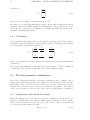
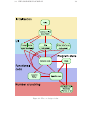
A schematic of the model-free optimisation protocol of Mandel et al., 1995 . 51
Model-free analysis using the diffusion seeded paradigm . . . . . . . . . . . 52
A schematic of the new model-free optimisation protocol . . . . . . . . . . . 54
8.1
8.2
8.3
The construction of the model-free gradient. . . . . . . . . . . . . . . . . . . 61
The model-free Hessian kite. . . . . . . . . . . . . . . . . . . . . . . . . . . . 63
χ2 dependencies of the values, gradients, and Hessians. . . . . . . . . . . . . 64
9.1
The core design of relax. . . . . . . . . . . . . . . . . . . . . . . . . . . . . . 133
xi
xii
LIST OF FIGURES
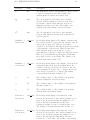
Abbreviations
AIC Akaike’s Information Criteria
AICc small sample size corrected AIC
BIC Bayesian Information Criteria
C(τ ) correlation function
χ2 chi-squared function
CSA chemical shift anisotropy
D the set of diffusion tensor parameters
Dk the eigenvalue of the spheroid diffusion tensor corresponding to the unique axis of the
tensor
D⊥ the eigenvalue of the spheroid diffusion tensor corresponding to the two axes perpendicular to the unique axis
Da the anisotropic component of the Brownian rotational diffusion tensor
Diso the isotropic component of the Brownian rotational diffusion tensor
Dr the rhombic component of the Brownian rotational diffusion tensor
Dratio the ratio of Dk to D⊥
Dx the eigenvalue of the Brownian rotational diffusion tensor in which the corresponding
eigenvector defines the x-axis of the tensor
Dy the eigenvalue of the Brownian rotational diffusion tensor in which the corresponding
eigenvector defines the y-axis of the tensor
Dz the eigenvalue of the Brownian rotational diffusion tensor in which the corresponding
eigenvector defines the z-axis of the tensor
ǫi elimination value
J(ω) spectral density function
NOE nuclear Overhauser effect
pdf probability distribution function
r bond length
xiii
xiv
R1 spin-lattice relaxation rate
R2 spin-spin relaxation rate
Rex chemical exchange relaxation rate
S 2 , Sf2 , and Ss2 model-free generalised order parameters
τe , τf , and τs model-free effective internal correlation times
τm global rotational correlation time
LIST OF FIGURES
Chapter 1
Introduction
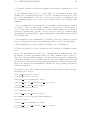
The program relax is designed for the study of the dynamics of proteins or other macromolecules though the analysis of NMR relaxation data. It is a community driven project
created by NMR spectroscopists for NMR spectroscopists. It supports exponential curve
fitting for the calculation of the R1 and R2 relaxation rates, calculation of the NOE,
reduced spectral density mapping, and the Lipari and Szabo model-free analysis.
The aim of relax is to provide a seamless and extremely flexible environment able to accept
input in any format produced by other NMR software, able to faultlessly create input files,
control, and read output from various programs including Modelfree and Dasha, output
results in many formats, and visualise the data by controlling programs such as Grace,
OpenDX, MOLMOL, and PyMOL. All data analysis tools from optimisation to model
selection to Monte Carlo simulations are inbuilt into relax. Therefore the use of additional
programs is optional.
The flexibility of relax arises from the choice of either relax’s scripting capabilities or its
Python prompt interface. Extremely complex scripts can be created from simple building
blocks to fully automate data analysis. A number of sample scripts have been provided
to help understand script construction. In addition, any of Python’s powerful features
or functions can be incorporated as the script is executed as an arbitrary Python source
file within relax’s environment. The modules of relax can also used as a vast library of
dynamics related functions by your own software.
relax is free software (free as in freedom) which is licenced under the GNU General Public
Licence (GPL). You are free to copy, modify, or redistribute relax under the terms of the
GPL.
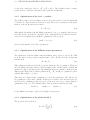
1.1
1.1.1
Program features
Literature
The primary references for the program relax are d’Auvergne and Gooley (2008a) and
d’Auvergne and Gooley (2008b).
1
2
CHAPTER 1. INTRODUCTION
Other literature related to the improved model-free analysis used within relax, which can
nevertheless be applied to other techniques such as SRLS, include model-free model selection (d’Auvergne and Gooley, 2003; Chen et al., 2004), model-free model elimination
(d’Auvergne and Gooley, 2006), the theory (d’Auvergne and Gooley, 2007) behind the
new model-free optimisation protocol (d’Auvergne and Gooley, 2008b), and the hybridisation of different models (Horne et al., 2007; d’Auvergne and Gooley, 2008b). Most of
these details can be found in the PhD thesis of d’Auvergne (2006).
1.1.2
Supported NMR theories
The following relaxation data analysis techniques are currently supported by relax:
• Model-free analysis (Lipari and Szabo, 1982a,b; Clore et al., 1990).
• Reduced spectral density mapping (Farrow et al., 1995; Lefevre et al., 1996).
• Exponential curve fitting (to find the R1 and R2 relaxation rates).
• Steady-state NOE calculation.
The future
At some time in the future the following techniques are planned to be implemented within
relax:
• Relaxation dispersion.
• SRLS – Slowly relaxing local structure (Tugarinov et al., 2001).
Because relax is free software, if you would like to contribute addition features, functions,
or modules which you have written for your own publications for the benefit of the field,
almost anything relating to molecular dynamics may be accepted. Please see the Open
Source chapter for more details.
1.1.3
Data analysis tools
The following tools are implemented as modular components to be used by any data
analysis technique:
• Numerous high-precision optimisation algorithms.
• Model selection (d’Auvergne and Gooley, 2003; Chen et al., 2004):
– Akaike’s Information Criteria (AIC).
– Small sample size corrected AIC (AICc).
– Bayesian or Schwarz Information Criteria (BIC).
1.1. PROGRAM FEATURES
3
– Bootstrap model selection.
– Single-item-out cross-validation (CV).
– Hypothesis testing ANOVA model selection (only the model-free specific technique of Mandel et al. (1995) is supported).
• Monte Carlo simulations (error analysis for all data analysis techniques).
• Model elimination – the removal of failed models prior to model selection (d’Auvergne and Gooley,
2006).
1.1.4
Data visualisation
The results of an analysis, or any data input into relax, can be visualised using a number
of programs:
MOLMOL 1D data can be mapped onto a structure either by the creation of MOLMOL
macros or by direct control of the program.
PyMOL 3D objects such as the diffusion tensor representation can be displayed with the
structure.
Grace any 2D data can be plotted.
OpenDX The chi-squared space of models with three parameters can be mapped and 3D
images of the space produced.
1.1.5
Interfacing with other programs
relax can create the input files, execute in-line, and then read the output of the following
programs. These programs can be used as optimisation engines replacing the minimisation
algorithms built into relax:
• Dasha (model-free analysis).
• Modelfree (model-free analysis).
1.1.6
The user interfaces (UI)
relax can be used through the following UIs:
The prompt this is the primary interface of relax. Rather than reinventing a new command language, relax’s interface is the powerful Python prompt. This gives the
power user full access to a proven programming language.
Scripting this provides a more powerful and flexible framework for controlling the program. The script will be executed as Python code enabling advanced programming
for automating data analysis. All the features available within the prompt environment are accessible to the script.
4
1.2
1.2.1
CHAPTER 1. INTRODUCTION
How to use relax
The prompt
The primary interface of relax is the prompt. After typing ‘relax’ within a terminal you
will be presented with
relax>
This is the Python prompt which has been tailored specifically for relax. You will hence
have full access, if desired, to the power of the Python programing language to manipulate
your data. You can for instance type
relax> print "Hello World"
the result being
relax> print "Hello World"
Hello World
relax>
Or using relax as a calculator
relax> (1.0 + (2 * 3))/10
0.69999999999999996
relax>
1.2.2
Python
relax has been designed such that knowledge about Python is not required to be able to
fully use the program. A few basics though will aid in understanding relax.
A number of simple programming axioms includes that of strings, integers, floating point
numbers, and lists. A string is text and within Python (as well as relax) this is delimited
by either single or double quotes. An integer is a number with no decimal point whereas
a float is a number with a decimal point. A list in Python (called an array in other
languages) is a list of anything separated by commas and delimited by square brackets,
an example is [0, 1, 2, ‘a’, 1.2143235].
Probably the most important detail is that functions in Python require brackets around
their arguments. For example
relax> minimise()
will commence minimisation however
relax> minimise
will do nothing.
The arguments to a function are simply a comma separated list within the brackets of the
function. For example to save the program’s current state type
relax> state.save(‘save’, force=True)
1.2. HOW TO USE RELAX
5
Two types of arguments exist in Python – standard arguments and keyword arguments.
The majority of arguments you will encounter within relax are keyword arguments however
you may, in rare cases, encounter a non-keyword argument. For these standard arguments
just type the values in, although they must be in the correct order. Keyword arguments
consist of two parts – the key and the value. For example the key may be file and
the value you would like to supply is ‘R1.out’. Various methods exist for supplying
this argument. Firstly you could simply type ‘R1.out’ into the correct position in the
argument list. Secondly you can type file=‘R1.out’. The power of this second option
is that argument order is unimportant. Therefore if you would like to change the default
value of the very last argument, you don’t have to supply values for all other arguments.
The only catch is that standard arguments must come before the keyword arguments.
1.2.3
User functions
For standard data analysis a large number of specially tailored functions called ‘user functions’ have been implemented. These are accessible from the relax prompt by simply
typing the name of the function. An example is ‘help()’. An alphabetical listing of all
accessible user functions together with full descriptions is presented later in this manual.
A few special objects which are available within the prompt are not actually functions.
These objects do not require brackets at their end for them to function. For example to
exit relax type
relax> exit
Another special object is that of the function class. This object is simply a container
which holds a number of user functions. You can access the user function within the class
by typing the name of the class, then a dot ‘.’, followed by the name of the user function.
An example is the user function for reading relaxation data out of a file and loading the
data into relax. The function is called ‘read’ and the class is called ‘relax data’. To
execute the function, type something like
relax> relax data.read(‘R1’, ‘600’, 600.0 * 1e6, ‘r1.600.out’)
On first usage the relax prompt can be quite daunting. Two features exist to increase the
usability of the prompt – the help system and tab completion.
1.2.4
The help system
For assistance in using a function simply type
help(function)
In addition to functions if
help(object)
is typed the help for the python object is returned. This system is similar to the help
function built into the python interpreter, which has been renamed to help python, with
the interactive component removed. For the standard interactive python help system type
help python()
6
1.2.5
CHAPTER 1. INTRODUCTION
Tab completion
Tab completion is implemented to prevent insanity as the function names can be quite
long – a deliberate feature to improve usability. The behaviour of the tab completion is
very similar to that of the bash prompt.
Not only is tab completion useful for preventing RSI but it can also be used for listing all
available functions. To begin with if you hit the [TAB] key without typing any text all
available functions will be listed (along with function classes and other python objects).
This extends to the exploration of user functions within a function class. For example to
list the user functions within the function class ‘model free’ type
relax> model free.
The dot character at the end is essential. After hitting the [TAB] key you should see
something like
relax> model free.
model free. class
model free. doc
model free. init
model free. module
model free. relax
model free. relax help
model free.create model
model free.delete
model free.remove tm
model free.select model
relax> model free.
All the objects beginning with an underscore are “hidden”, they contain information
about the function class and should be ignored. From the listing the user functions
‘copy’, ‘create model’, ‘delete’, ‘remove tm’, and ‘select model’ contained within
‘model free’ are all visible.
1.2.6
The data pipe
Within relax all user functions operate on data stored within the current data pipe. This
pipe stores data is input, processed, or output as user functions are called. There are
different types of data pipe for different analyses, e.g. a reduced spectral density mapping
pipe, a model-free pipe, an exponential curve-fitting pipe, etc. Multiple data pipes can be
created within relax and various operations performed in sequence on these pipes. This is
useful for operations such as model selection whereby the function ‘model selection’ can
operate on a number of pipes corresponding to different models and then assign the results
to a newly created pipe. When running relax you choose which pipe you are currently in
by using the ‘pipe.switch’ user function to jump between pipes.
The flow of data through relax can be thought of as travelling through these pipes. User
functions exist to transfer data between these pipes and other functions combine data
from multiple pipes into one or vice versa. The simplest invocation of relax would be the
7
1.2. HOW TO USE RELAX
creation of a single data pipe and with the data being processed as it is passing through
this pipe.
The primary method for creating a data pipe is through the user function ‘pipe.create’.
For example
relax> pipe.create(‘m1’, ‘mf’)
will create a model-free data pipe labelled ‘m1’. The following is a table of all the types
which can be assigned to a data pipe.
Data pipe type
Description
‘jw’
‘mf’
‘N-state’
‘noe’
‘relax fit’
‘srls’
Reduced spectral density mapping
Model-free data analysis
N-state model of domain motions
Steady state NOE calculation
Relaxation curve-fitting
SRLS analysis
Currently the NOE calculation, relaxation curve-fitting, model-free analysis, and reduced
spectral density mapping features of relax are implemented (if this documentation is out
of date then you may be able to do a lot more).
1.2.7
Scripting
What ever is done within the prompt is also accessible through scripting. Just type your
commands into a text file and then at the terminal type
$ relax your script
An example of a simple script which will minimise the model-free model ‘m4’ after loading
six relaxation data sets is
# Create the data pipe.
name = ‘m4’
pipe.create(name, ‘mf’)
# Nuclei type
nuclei(‘N’)
# Load the sequence.
sequence.read(‘noe.500.out’)
# Load the relaxation data.
relax data.read(‘R1’, ‘600’, 600.0 * 1e6, ‘r1.600.out’)
relax data.read(‘R2’, ‘600’, 600.0 * 1e6, ‘r2.600.out’)
relax data.read(‘NOE’, ‘600’, 600.0 * 1e6, ‘noe.600.out’)
relax data.read(‘R1’, ‘500’, 500.0 * 1e6, ‘r1.500.out’)
relax data.read(‘R2’, ‘500’, 500.0 * 1e6, ‘r2.500.out’)
8
CHAPTER 1. INTRODUCTION
relax data.read(‘NOE’, ‘500’, 500.0 * 1e6, ‘noe.500.out’)
# Setup other values.
diffusion tensor.init((2e-8, 1.3, 60, 290), param types=1, axial type=‘prolate’,
fixed=True)
value.set(1.02 * 1e-10, ‘bond length’)
value.set(-160 * 1e-6, ‘csa’)
value.set(‘15N’, ‘heteronucleus’)
value.set(‘1H’, ‘proton’)
# Select a preset model-free model.
model free.select model(model=name)
# Grid search.
grid search(inc=11)
# Minimise.
minimise(‘newton’)
# Finish.
results.write(file=‘results’, force=True)
state.save(‘save’, force=True)
Scripting is much more powerful than the prompt as advanced Python programming can
be employed (see the file ‘full analysis.py’ in the ‘sample scripts’ directory for an example).
1.2.8
Sample scripts
A few sample scripts have been provided in the directory ‘sample scripts’. These can be
copied and modified for different types of data analysis.
1.2.9
The test suite
To test that the program functions correctly, relax possesses an inbuilt test suite. The
suite is a collection of simple tests which execute or probe different parts of the program
checking that the software runs without problem. The test suite is executed by running
relax using the command ‘relax --test-suite’.
1.2.10
The GUI
relax has been designed primarily for scripting and, as such, no graphical user interface
(GUI) currently exists. The internal structure of the program has been specifically designed
so any type of control mechanism can be easily added, including a GUI, therefore in the
future one may be written. A GUI will, however, detract from the power and flexibility
inherent in the control by scripting.
1.3. USAGE OF THE NAME RELAX
1.2.11
9
Access to the internals of relax
To enable advanced Python scripting and control many parts of relax have been designed
in an object oriented fashion. If you would like to play with internals of the program the
entirety of relax is accessible by importation. For example all data is contained within
the object called the relax data store which, to be able to access it, needs be imported by
typing:
relax> from data import Data as relax data store
This is a dictionary type object which contains the multiple data pipes. All of relax’s
packages, modules, functions, and classes are also accessible by import statements. For
example to create a rotation matrix from three Euler angles in the z-y-z notation, type:
relax> alpha = 0.1342
relax> beta = 1.0134
relax> gamma = 2.4747
relax> from maths fns.rotation matrix import R euler zyz
relax> from numpy import float64, zeros
relax> R = zeros((3,3), float64)
relax> R euler zyz(R, alpha, beta, gamma)
relax> R
1.3
Usage of the name relax
The program relax is so relaxed that the first letter should always be in lower case!
10
CHAPTER 1. INTRODUCTION
Chapter 2
Installation instructions
2.1
Dependencies
The following packages need to be installed before using relax:
Python: Version 2.4 or higher (although any 2.x version may work).
Numeric: Version 21 or higher.
ScientificPython: Version 2.2 or higher.
Optik: Version 1.4 or higher. This is only needed if running python <= 2.2.
Older versions of these packages may work, use them at your own risk. If, for older
dependency versions, errors do occur please submit a bug report to the bug tracker at
https://gna.org/bugs/?group=relax. That way a solution may be created for the next
relax release.
2.2
2.2.1
Installation
The precompiled verses source distribution
Two types of software packages are available for download – the precompiled and source
distribution. Currently only relaxation curve-fitting requires compilation to function and
all other features of relax will be fully functional without compilation. If relaxation curvefitting is required but no precompiled version of relax exists for your operating system
or architecture then, if a C compiler is present, the C code can be compiled into the
shared objects files *.so which are loaded as modules into relax. To build these modules
the Sconstruct system from http://scons.org/ is required. This software only depends on
Python which is essential for running relax anyway. Once Sconstruct is installed type
$ scons
11
12
CHAPTER 2. INSTALLATION INSTRUCTIONS
in the base directory where relax has been installed and the C modules should, hopefully,
compile without any problems. Otherwise please submit a bug report to the bug tracker
at https://gna.org/bugs/?group=relax.
2.2.2
Installation on GNU/Linux
To install the program relax on a GNU/Linux system download either the precompiled
distribution labelled relax-x.x.x.GNU-Linux.arch.tar.bz2 matching your machine architecture or the source distribution relax-x.x.x.src.tar.bz2. A number of installation
methods are possible. The simplest way is to switch to the user ‘root’, unpack and decompress the archive within the /usr/local directory by typing, for instance
$ tar jxvf relax-x.x.x.GNU-Linux.i686.tar.bz2
then create a symbolic link in /usr/local/bin by moving to that directory and typing
$ ln -s ../relax/relax .
and finally running relax to create the byte-compiled Python *.pyc files to speed up the
start time of relax by typing
$ relax --test
Alternatively if the Sconstruct system is installed typing
$ scons install
in the relax base directory will create a directory in /usr/local/ called relax, copy
all the uncompressed and untarred files into this directory, create a symbolic link in
/usr/local/bin to the file /usr/local/relax/relax, and then finally run relax to create the byte-compiled Python *.pyc. To change the installation path to a non-standard
location the Sconstruct script sconstruct in the base relax directory should be modified
by changing the variable INSTALL PATH to point to the desired location.
2.2.3
Installation on MS Windows
In addition to the above dependencies, running relax on MS Windows requires a number
of additional programs. These include:
pyreadline: Version 1.3 or higher (download).
ctypes: The pyreadline package requires ctypes (download).
To install, simply download the pre-compiled binary distribution relax-x.x.x.Win32.zip
or the source distribution relax-x.x.x.src.zip and extract the files to C:\Program
Files\relax-x.x.x. Then add this directory to the system environment path (in Windows XP, right click on ‘My Computer’, go to ‘Properties’, click on the ‘Advanced’ tab, and
click on the ‘Envirnment Variables’ button. Then double click on the ‘Path’ system variable and add the text “;C:\Program Files\relax-x.x.x” to the end of variable value field.
The Python installation must also be located on the path (add the text “;C:\Program
2.3. OPTIONAL PROGRAMS
13
Files\Python24”, changing the text to point to the correct directory, to the field). To run
the program from any directory inside the Windows command prompt (or dos prompt)
type:
C:\> relax
2.2.4
Installation on Mac OS X
Please write me if you know how to do this!
2.2.5
Installation on your OS
Please write me if you know how to do this!
2.2.6
Running a non-compiled version
Compilation of the C code is not essential for running relax, however certain features of
the program will be disabled. Currently only the exponential curve-fitting for determining
the R1 and R2 relaxation rates requires compilation. To run relax without compilation
install the dependencies detailed above, download the source distribution which should be
named relax-x.x.x.src.tar.bz2, extract the files, and then run the file called relax in
the base directory.
2.3
Optional programs
The following is a list of programs which can be used by relax although they are not
essential for normal use.
2.3.1
Grace
Grace is a program for plotting two dimensional data sets in a professional looking manner. It is used to visualise parameter values. It can be downloaded from
http://plasma-gate.weizmann.ac.il/Grace/.
2.3.2
OpenDX
Version 4.1.3 or compatible. OpenDX is used for viewing the output of the space mapping
function and is executed by passing the command dx to the command line with various
options. The program is designed for visualising multidimensional data and can be found
at http://www.opendx.org/.
14
2.3.3
CHAPTER 2. INSTALLATION INSTRUCTIONS
Molmol
Molmol is used for viewing the PDB structures loaded into the program and to display
parameter values mapped onto the structure.
2.3.4
PyMOL
PDB structures can also be viewed using PyMOL. Although the mapping of parameter
values onto the structure is not yet supported, this program can be used to display geometric objects generated by relax for representing physical concepts such as the diffusion
tensor.
2.3.5
Dasha
Dasha is a program used for model-free analysis of NMR relaxation data. It can be used as
an optimisation engine to replace the minimisation algorithms implemented within relax.
2.3.6
Modelfree4
Art Palmer’s Modelfree4 program is also designed for model-free analysis and can be used
as an optimisation engine to replace relax’s high precision minimisation algorithms.
Chapter 3
Open source infrastructure
3.1
The relax web sites
The main web site for relax is http://nmr-relax.com. From these pages general information
about the program, links to the latest documentation, links to the most current software
releases, and information about the mailing lists are available. There are also Google search
capabilities built into the pages for searching both the HTML version of the manual and
the archives of the mailing lists.
The relax web site is hosted by the Gna! project (https://gna.org/) which is described as
“a central point for development, distribution and maintenance of Libre Software (Free
Software) projects”. relax is a registered Gna! project and its primary Gna! web site is
https://gna.org/projects/relax. This site contains many more technical details than the
main web site.
3.2
The mailing lists
A number of mailing lists have been created covering different aspects of relax. These
include the announcement list, the relax users list, the relax development list, and the
relax committers list.
3.2.1
relax-announce
The relax announcement list “relax-announce at gna.org” is reserved for important announcements about the program including the release of new program versions. The
amount of traffic on this list is relatively low. If you would like to receive information about relax you can subscribe to the list by vising the information page at
https://mail.gna.org/listinfo/relax-announce/. Previous announcements can be viewed
at https://mail.gna.org/public/relax-announce/.
15
16
3.2.2
CHAPTER 3. OPEN SOURCE INFRASTRUCTURE
relax-users
If you would like to ask questions about relax, discuss certain features, receive help, or to
communicate on any other subject related to relax the mailing list “relax-users at gna.org”
is the place to post your message. To subscribe to the list go to the relax-users information
page at https://mail.gna.org/listinfo/relax-users/. You can also browse the mailing list
archives at https://mail.gna.org/public/relax-users/.
3.2.3
relax-devel
A second mailing list exists for posts relating to the development of relax. The list
is “relax-devel at gna.org” and to subscribe go to the relax-devel information page at
https://mail.gna.org/listinfo/relax-devel/. Feature requests, program design, or any other
posts relating to relax’s structure or code should be sent to this list instead. The mailing
list archives can be browsed at https://mail.gna.org/public/relax-devel/.
3.2.4
relax-commits
One last mailing list is the relax commits list. This list is reserved for automatically
generated posts created by the version control software which looks after the relax source
code and these web pages. If you would like to become a developer you can subscribe to
the list at relax-commits information page https://mail.gna.org/listinfo/relax-commits/.
The list can also be browsed at https://mail.gna.org/public/relax-commits/.
3.2.5
Replying to a message
When replying to a message on these lists remember to hit ‘respond to all’ so that the
mailing list is included in the CC field. Otherwise your message will only be sent to the
original poster and not return back to the list. Only messages to relax-users and relaxdevel will be accepted. If you are using Gmail’s web based interface, please do not click
on ‘Edit Subject’ as this currently mangles the email headers, creates a new thread on the
mailing list, and makes it difficult to follow the thread.
3.3
Reporting bugs
One of the philosophies in the construction of relax is that if there is something which
is not immediately obvious then that is considered a design bug. If any flaws in relax are uncovered including general design flaws, bugs in the code, or documentation
issues these can be reported within relax’s bug tracker system. The link to submit
a bug is https://gna.org/bugs/?group=relax&func=additem while the main page for
browsing, submitting, viewing the statistics, or searching through the database is at
https://gna.org/bugs/?group=relax. Please do not report bugs to personal email addresses or to the mailing lists.
3.4. LATEST SOURCES – THE RELAX REPOSITORIES
17
When reporting a bug please include as much information as possible so that the problem
can be reproduced. Include information such as the release version or the revision number
if the repository sources are being used. Also include all the steps performed in order to
trigger the bug. Attachment of files is allowed so scripts and subsets of the input data
can be included. However please do not attach large files to the report. Prior to reporting
the bug try to make sure that the problem is indeed a bug and if you have any doubts
please feel free to ask on the relax-users mailing list. To avoid duplicates be sure that the
bug has not already been submitted to the bug tracker. You can search the bugs from the
page https://gna.org/project/search.php?group=relax.
Once the bug has been confirmed by one of the relax developers you may speed up the
resolution of the problem by trying to fixing the bug yourself. If you do wish to play with
the source code and try to fix the issue see the relax development chapter of this manual
on how to check out the latest sources, how to generate a patch (which is just the output
of diff in the ‘unified’ format), and the guidelines for the format of the code.
3.4
Latest sources – the relax repositories
relax’s source code is kept within a version control system called Subversion
(http://subversion.tigris.org/). Subversion or SVN allows fine control over the development of the program. The repository contains all information about every change ever
made to the program. To learn more about the system the Subversion book located at
http://svnbook.red-bean.com/ is a good place to start. The contents of the relax repository can be viewed on-line at http://svn.gna.org/viewcvs/relax/. The current sources,
assuming that the most recent minor version number is 1.2, can be downloaded using the
SVN protocol by typing
$ svn co svn://svn.gna.org/svn/relax/1.2 relax
however if this does not work, try the command
$ svn co http://svn.gna.org/svn/relax/1.2 relax
to download using the HTTP protocol. The entire relax repository is backed up daily to
http://svn.gna.org/daily/relax.dump.gz.
3.5
News
Summaries of the latest news on relax can be found on the relax web site
https://gna.org/projects/relax. However more information can be found at the dedicated
news page https://gna.org/news/?group=relax.
3.6
The relax distribution archives
The relax distribution archives, the files to download to install relax, can be found at
http://download.gna.org/relax/. If a compiled binary distribution for your architecture
18
CHAPTER 3. OPEN SOURCE INFRASTRUCTURE
does not exist you are welcome to create this distribution yourself and submit it for inclusion in the relax project. To do this a number of steps are required. Firstly, the code
to each relax release or version resides in the ‘tags’ directory of the relax repository. To
check out version 1.2.0 for example type
$ svn co svn://svn.gna.org/svn/relax/tags/1.2.0 relax
Again the sources are available through HTTP by typing
$ svn co http://svn.gna.org/svn/relax/tags/1.2.0 relax
The binary distribution can then be created for your architecture by shifting to the main
directory of the checked out sources and typing
$ cd relax
$ scons binary dist
At the end SCons will attempt to make a GPG signature for the newly created archive.
However this will fail as the current relax private GPG key is not available for security reasons. If the SCons command fails, excluding the GPG signing, please submit
a bug report with as much information possible including the details described next to
https://gna.org/bugs/?group=relax&func=additem (the python and SCons version numbers may also be useful). Once the file has been created post a message to the relax
development mailing list describing the compilation and the creation of the archive, the
relax version number, the machine architecture, operating system, and the name of the
new file. Do not attach the file though. You will then receive a response explaining where
to send the file to. For security the archive will be thoroughly checked and if the source
code is identical to that in the repository and the C modules are okay, the file will be GPG
signed and uploaded to http://download.gna.org/relax/.
Chapter 4
Calculating the NOE
4.1
Introduction
The calculation of NOE values is a straight forward and quick procedure which involves
two components – the calculation of the value itself and the calculation of the errors. To
understand the steps involved the execution of a sample NOE calculation script will be
followed in detail.
4.2
The sample script
# Script for calculating NOEs.
# Create the data pipe.
pipe.create(‘NOE’, ‘noe’)
# Load the sequence from a PDB file.
structure.read pdb(name, ‘Ap4Aase new 3.pdb’)
structure.load spins(spin id=‘@N’)
# Load the reference spectrum and saturated spectrum peak intensities.
noe.read(file=‘ref.list’, spectrum type=‘ref’)
noe.read(file=‘sat.list’, spectrum type=‘sat’)
# Set the errors.
noe.error(error=3600, spectrum type=‘ref’)
noe.error(error=3000, spectrum type=‘sat’)
# Individual residue errors.
noe.error(error=122000, spectrum type=‘ref’, res num=114)
noe.error(error=8500, spectrum type=‘sat’, res num=114)
# Deselect unresolved residues.
deselect.read(file=‘unresolved’)
19
20
CHAPTER 4. CALCULATING THE NOE
# Calculate the NOEs.
calc()
# Save the NOEs.
value.write(param=‘noe’, file=‘noe.out’, force=True)
# Create grace files.
grace.write(y data type=‘ref’, file=‘ref.agr’, force=True)
grace.write(y data type=‘sat’, file=‘sat.agr’, force=True)
grace.write(y data type=‘noe’, file=‘noe.agr’, force=True)
# View the grace files.
grace.view(file=‘ref.agr’)
grace.view(file=‘sat.agr’)
grace.view(file=‘noe.agr’)
# Write the results.
results.write(file=‘results’, dir=None, force=True)
# Save the program state.
state.save(‘save’, force=True)
4.3
Initialisation of the data pipe
The data pipe is simply created by the command
pipe.create(‘NOE’, ‘noe’)
This user function will then create a NOE calculation specific data pipe labelled ‘NOE’.
The second argument sets the pipe type to that of the NOE calculation. Setting the pipe
type is important so that the program knows which user functions are compatible with
the data pipe, for example the function minimise() is meaningless in this sample script
as the NOE values are directly calculated rather than optimised.
4.4
Loading the data
The first thing which need to be completed prior to any residue specific command is to
generate the sequence from a PDB file. In this case the command
structure.read pdb(name, ‘Ap4Aase new 3.pdb’)
will load the PDB file ‘Ap4Aase new 3.pdb’ into relax. Then
structure.load spins(spin id=‘@N’)
will generate the molecule, residue, and spin sequence for the current data pipe. In this
situation there will be a single spin system per residue generated corresponding to the
backbone amide nitrogens. Although the PDB coordinates have been loaded into the
program, the structural information serves no purpose when calculating NOE values.
4.5. SETTING THE ERRORS
21
The next two commands
noe.read(file=‘ref.list’, spectrum type=‘ref’)
noe.read(file=‘sat.list’, spectrum type=‘sat’)
load the peak heights of the reference and saturated NOE experiments (although the
volume could be used instead). The keyword argument format has not been specified
hence the default format of a Sparky peak list (saved after typing ‘lt’) is assumed. If
the program XEasy was used to analyse the spectra the argument format=‘xeasy’ is
necessary. The first column of the file should be the Sparky assignment string and it is
assumed that the 4th column contains either the peak height or peak volume. If you have
any other format you would like read by relax please send an email to the relax development
mailing list detailing the software used, the format of the file (specifically where the residue
number and peak intensity are located), and possibly attaching an example of the file itself.
4.5
Setting the errors
In this example the errors where measured from the base plain noise. The Sparky RMSD
function was used to estimate the maximal noise levels across the spectrum in regions
containing no peaks. For the reference spectrum the RMSD was approximately 3600
whereas in the saturated spectrum the RMSD was 3000. These errors are set by the
commands
noe.error(error=3600, spectrum type=‘ref’)
noe.error(error=3000, spectrum type=‘sat’)
For the residue G114, the noise levels are significantly increased compared to the rest of
the protein as the peak is located close to the water signal. The higher errors for this
residue are specified by the commands
noe.error(error=122000, spectrum type=‘ref’, res num=114)
noe.error(error=8500, spectrum type=‘sat’, res num=114)
4.6
Unresolved residues
As the peaks of certain residues overlap to such an extent that the heights cannot be
resolved, a simple text file was created called unresolved in which each line consists of a
single residue number. By using the command
deselect.read(name, file=‘unresolved’)
all residues in the file unresolved are excluded from the analysis.
4.7
The NOE
At this point the NOE can be calculated. The user function
22
CHAPTER 4. CALCULATING THE NOE
calc()
will calculate both the NOE and the errors. The NOE value will be calculated using the
formula
Isat
,
(4.1)
N OE =
Iref
where Isat is the intensity of the peak in the saturated spectrum and Iref is that of the
reference spectrum. The error is calculated by
s
(σsat · Iref )2 + (σref · Isat )2
σN OE =
,
(4.2)
Iref
where σsat and σref are the peak intensity errors in the saturated and reference spectra
respectively. To create a file of the NOEs the command
value.write(param=‘noe’, file=‘noe.out’, force=True)
will create a file called noe.out with the NOE values and errors. The force flag will cause
any file with the same name to be overwritten. An example of the format of noe.out is
Num
1
2
3
4
5
6
7
8
9
10
11
12
13
14
4.8
Name
GLY
PRO
LEU
GLY
SER
MET
ASP
SER
PRO
PRO
GLU
GLY
TYR
ARG
Value
None
None
None
0.12479588727508535
0.42240815792914105
0.45281703194372114
0.60727570079478255
0.63871921623680161
None
None
None
0.92927160307645906
0.88832516377296256
0.84945042565860407
Error
None
None
None
0.020551827436105764
0.02016346825976852
0.026272719841642134
0.032369427242382849
0.024695665815261791
None
None
None
0.059569089743604184
0.044119641308479306
0.060533543601110441
Viewing the results
Any two dimensional data set can be plotted in relax in conjunction with the program
Grace. The program is also known as Xmgrace and was previously known as ACE/gr or
Xmgr. The highly flexible relax user function grace.write is capable of producing 2D
plots of any x-y data sets. The three commands
grace.write(y data type=‘ref’, file=‘ref.agr’, force=True)
grace.write(y data type=‘sat’, file=‘sat.agr’, force=True)
grace.write(y data type=‘noe’, file=‘noe.agr’, force=True)
create three separate plots of the peak intensity of the reference and saturated spectra as
well as the NOE. The x-axis in all three defaults to the residue number. As the x and
y-axes can be any parameter the command
23
4.8. VIEWING THE RESULTS
1
0.9
0.8
0.7
NOE
0.6
0.5
0.4
0.3
0.2
0.1
0
0
10
20
30
40
50
60
70
80
90
100 110 120 130 140 150 160 170
Residue number
Figure 4.1: A Grace plot of the NOE value and error against the residue number. This is
an example of the output of the user function grace.write().
grace.write(x data type=‘ref’, y data type=‘sat’, file=‘ref vs sat.agr’, force=True)
would create a plot of the reference verses the saturated intensity with one point per
residue. Returning to the sample script three Grace data files are created ref.agr,
sat.agr, and noe.agr and placed in the default directory ./grace. These can be visualised by opening the file within Grace. However relax will do that for you with the
commands
grace.view(file=‘ref.agr’)
grace.view(file=‘sat.agr’)
grace.view(file=‘noe.agr’)
An example of the output after modifying the axes is shown in figure 4.1.
24
CHAPTER 4. CALCULATING THE NOE
Chapter 5
The R1 and R2 relaxation rates –
relaxation curve-fitting
5.1
Introduction
Relaxation curve-fitting involves a number of steps including the loading of data, the
calculation of both the average peak intensity across replicated spectra and the standard
deviations of those peak intensities, selection of the experiment type, optimisation of the
parameters of the fit, Monte Carlo simulations to find the parameter errors, and saving
and viewing the results. To simplify the process a sample script will be followed step by
step as was done with the NOE calculation.
5.2
The sample script
# Script for relaxation curve-fitting.
# Create the ‘rx’ data pipe.
pipe.create(‘rx’, ‘relax fit’)
# Load the backbone amide 15N spins from a PDB file.
structure.read pdb(‘Ap4Aase new 3.pdb’)
structure.load spins(spin id=‘@N’)
# Load the peak intensities.
relax fit.read(file=‘T2 ncyc1.list’, relax time=0.0176)
relax fit.read(file=‘T2 ncyc1b.list’, relax time=0.0176)
relax fit.read(file=‘T2 ncyc2.list’, relax time=0.0352)
relax fit.read(file=‘T2 ncyc4.list’, relax time=0.0704)
relax fit.read(file=‘T2 ncyc4b.list’, relax time=0.0704)
relax fit.read(file=‘T2 ncyc6.list’, relax time=0.1056)
relax fit.read(file=‘T2 ncyc9.list’, relax time=0.1584)
relax fit.read(file=‘T2 ncyc9b.list’, relax time=0.1584)
25
26
CHAPTER 5. RELAXATION CURVE-FITTING
relax fit.read(file=‘T2 ncyc11.list’, relax time=0.1936)
relax fit.read(file=‘T2 ncyc11b.list’, relax time=0.1936)
# Calculate the peak intensity averages and the standard deviation of all spectra.
relax fit.mean and error()
# Deselect unresolved residues.
deselect.read(file=‘unresolved’)
# Set the relaxation curve type.
relax fit.select model(‘exp’)
# Grid search.
grid search(inc=11)
# Minimise.
minimise(‘simplex’, scaling=False, constraints=False)
# Monte Carlo simulations.
monte carlo.setup(number=500)
monte carlo.create data()
monte carlo.initial values()
minimise(‘simplex’, scaling=False, constraints=False)
monte carlo.error analysis()
# Save the relaxation rates.
value.write(param=‘rx’, file=‘rx.out’, force=True)
# Grace plots of the relaxation rate.
grace.write(y data type=‘rx’, file=‘rx.agr’, force=True)
grace.view(file=‘rx.agr’)
# Save the program state.
state.save(file=‘rx.save’, force=True)
5.3
Initialisation of the data pipe and loading of the data
The start of this sample script is very similar to that of the NOE calculation on page 20.
The command
pipe.create(‘rx’, ‘relax fit’)
initialises the data pipe labelled ‘rx’. The data pipe type is set to relaxation curve-fitting
by the argument ‘relax fit’. The backbone amide nitrogen sequence is extracted from
a PDB file using the same commands as the NOE calculation script
structure.read pdb(name, ‘Ap4Aase new 3.pdb’)
structure.load spins(spin id=‘@N’)
27
5.4. THE REST OF THE SETUP
To load the peak intensities into relax the user function relax fit.read is executed. Two
important keyword arguments to this command are the file name and the relaxation time
period of the experiment in seconds. It is assumed that the file format is that of a Sparky
peak list. Using the format argument, this can be changed to XEasy text window output
format. To be able to import any other type of format please send an email to the relax
development mailing list with the details of the format. Adding support for new formats
is trivial. The following series of commands will load peak intensities from six different
relaxation periods, four of which have been duplicated
relax fit.read(file=‘T2 ncyc1.list’, relax time=0.0176)
relax fit.read(file=‘T2 ncyc1b.list’, relax time=0.0176)
relax fit.read(file=‘T2 ncyc2.list’, relax time=0.0352)
relax fit.read(file=‘T2 ncyc4.list’, relax time=0.0704)
relax fit.read(file=‘T2 ncyc4b.list’, relax time=0.0704)
relax fit.read(file=‘T2 ncyc6.list’, relax time=0.1056)
relax fit.read(file=‘T2 ncyc9.list’, relax time=0.1584)
relax fit.read(file=‘T2 ncyc9b.list’, relax time=0.1584)
relax fit.read(file=‘T2 ncyc11.list’, relax time=0.1936)
relax fit.read(file=‘T2 ncyc11b.list’, relax time=0.1936)
5.4
The rest of the setup
Once all the peak intensity data has been loaded a few calculations are required prior
to optimisation. Firstly the peak intensities for individual residues needs to be averaged
across replicated spectra. The peak intensity errors also have to be calculated using the
standard deviation formula. These two operations are executed by the user function
relax fit.mean and error()
Any residues which cannot be resolved due to peak overlap were included in a file called
‘unresolved’. This file consists solely of one residue number per line. These residues are
excluded from the analysis by the user function
deselect.read(file=‘unresolved’)
Finally the experiment type is specified by the command
relax fit.select model(‘exp’)
The argument ‘exp’ sets the relaxation curve to a two parameter {Rx , I0 } exponential
which decays to zero. The formula of this function is
I(t) = I0 e−Rx ·t ,
(5.1)
where I(t) is the peak intensity at any time point t, I0 is the initial intensity, and Rx is
the relaxation rate (either the R1 or R2 ). Changing the user function argument to ‘inv’
will select the inversion recovery experiment. This curve consists of three paremeters {R1 ,
I0 , I∞ } and does not decay to zero. The formula is
I(t) = I∞ − I0 e−R1 ·t .
(5.2)
28
5.5
CHAPTER 5. RELAXATION CURVE-FITTING
Optimisation
Now that everything has been setup minimision can be used to optimise the parameter
values. Firstly a grid search is applied to find a rough starting position for the subsequent
optimisation algorithm. Eleven increments per dimension of the model (in this case the
two dimensions {Rx , I0 }) is sufficient. The user function for executing the grid search is
grid search(inc=11)
The next step is to select one of the minimisation algorithms to optimise the model parameters. Currently for relaxation curve-fitting only simplex minimisation is supported.
This is because the relaxation curve-fitting C module is incomplete only implementing the
chi-squared function. The chi-squared gradient (the vector of first partial derivatives) and
chi-squared Hessian (the matrix of second partial derivatives) are not yet implemented in
the C modules and hence optimisation algorithms which only employ function calls are
supported. Simplex minimisation is the only technique in relax which fits this criteron. In
addition constraints cannot be used as the constraint algorithm is dependent on gradient
calls. Therefore the minimisation command for relaxation curve-fitting is forced to be
minimise(‘simplex’, constraints=False)
5.6
Error analysis
Only one technique adequately estimates parameter errors when the parameter values
where found by optimisation – Monte Carlo simulations. In relax this can be implemented
by using a series of functions from the monte carlo user function class. Firstly the number
of simulations needs to be set
monte carlo.setup(number=500)
For each simulation, randomised relaxation curves will be fit using exactly the same
methodology as the original exponential curves. These randomised curves are created
by back calculation from the fitted model parameter values and then each point on the
curve randomised using the error values set earlier in the script
monte carlo.create data()
As a grid search for each simulation would be too computationally expensive, the starting
point for optimisation for each simulation can be set to the position of the optimised
parameter values of the model
monte carlo.initial values()
Then exactly the same optimisation as was used for the model can be performed
minimise(‘simplex’, constraints=False)
The parameter errors are then determined as the standard deviation of the optimised
parameter values of the simulations
monte carlo.error analysis()
5.7. FINISHING OFF
5.7
29
Finishing off
To finish off, the script first saves the relaxation rates together with their errors in a simple
text file
value.write(param=‘rx’, file=‘rx.out’, force=True)
Grace plots are created and viewed
grace.write(y data type=‘rx’, file=‘rx.agr’, force=True)
grace.view(file=‘rx.agr’)
and finally the program state is saved for future reference
state.save(file=‘rx.save’, force=True)
30
CHAPTER 5. RELAXATION CURVE-FITTING
Chapter 6
Model-free analysis
6.1
6.1.1
Theory
The chi-squared function – χ2 (θ)
For the minimisation of the model-free models a chain of calculations, each based on a
different theory, is required. At the highest level the equation which is actually minimised
is the chi-squared function
n
X
(Ri − Ri (θ))2
,
(6.1)
χ2 (θ) =
σi2
i=1
where the index i is the summation index ranging over all the experimentally collected
relaxation data of all residues used in the analysis; Ri belongs to the relaxation data set R
for an individual residue, a collection of residues, or the entire macromolecule and includes
the R1 , R2 , and NOE data at all field strengths; Ri (θ) is the back-calculated relaxation
value belonging to the set R(θ); θ is the model parameter vector which when minimised
is denoted by θ̂; and σi is the experimental error.
The significance of the chi-squared equation (6.1) is that the function returns a single value
which is then minimised by the optimisation algorithm to find the model-free parameter
values of the given model.
6.1.2
The transformed relaxation equations – Ri (θ)
The chi-squared equation is itself dependent on the relaxation equations through the backcalculated relaxation data R(θ). Letting the relaxation values of the set R(θ) be the
R1 (θ), R2 (θ), and NOE(θ) an additional layer of abstraction can be used to simplify the
calculation of the gradients and Hessians. This involves decomposing the NOE equation
into the cross relaxation rate constant σNOE (θ) and the auto relaxation rate R1 (θ). Taking
31
32
CHAPTER 6. MODEL-FREE ANALYSIS
equation (6.6) below the transformed relaxation equations are
R1 (θ) = R′1 (θ),
(6.2a)
R′2 (θ),
(6.2b)
R2 (θ) =
NOE(θ) = 1 +
γH σNOE (θ)
.
γX R1 (θ)
(6.2c)
whereas the relaxation equations are the R1 (θ), R2 (θ), σNOE (θ).
6.1.3
The relaxation equations – R′i (θ)
The relaxation values of the set R′ (θ) include the spin-lattice, spin-spin, and crossrelaxation rates at all field strengths. These rates are respectively (Abragam, 1961)
R1 (θ) = d J(ωH − ωX ) + 3J(ωX ) + 6J(ωH + ωX ) + cJ(ωX ),
(6.3a)
d
4J(0) + J(ωH − ωX ) + 3J(ωX ) + 6J(ωH )
R2 (θ) =
2
c
+ 6J(ωH + ωX ) +
4J(0) + 3J(ωX ) + Rex ,
(6.3b)
6
σNOE (θ) = d 6J(ωH + ωX ) − J(ωH − ωX ) ,
(6.3c)
where J(ω) is the power spectral density function and Rex is the relaxation due to chemical
exchange. The dipolar and CSA constants are defined in SI units as
d=
1 µ0 2 (γH γX ~)2
,
4 4π
hr 6 i
(ωH ∆σ)2
c=
,
3
(6.4)
(6.5)
where µ0 is the permeability of free space, γH and γX are the gyromagnetic ratios of the
H and X spins respectively, ~ is Plank’s constant divided by 2π, r is the bond length, and
∆σ is the chemical shift anisotropy measured in ppm. The cross-relaxation rate σNOE is
related to the steady state NOE by the equation
NOE(θ) = 1 +
6.1.4
γH σNOE (θ)
.
γX R1 (θ)
(6.6)
The spectral density functions – J(ω)
The relaxation equations are themselves dependent on the calculation of the spectral
density values J(ω). Within model-free analysis these are modelled by the original modelfree formula (Lipari and Szabo, 1982a,b)
!
k
S2
(1 − S 2 )(τe + τi )τe
2 X
ci · τi
+
,
J(ω) =
5
1 + (ωτi )2 (τe + τi )2 + (ωτe τi )2
i=−k
(6.7)
33
6.1. THEORY
where S 2 is the square of the Lipari and Szabo generalised order parameter and τe is
the effective correlation time. The order parameter reflects the amplitude of the motion
and the correlation time in an indication of the time scale of that motion. The theory
was extended by Clore et al. (1990) by the modelling of two independent internal motions
using the equation
k
(1 − Sf2 )(τf + τi )τf
2 X
S2
+
J(ω) =
ci · τi
5
1 + (ωτi )2 (τf + τi )2 + (ωτf τi )2
i=−k
+
(Sf2 − S 2 )(τs + τi )τs
(τs + τi )2 + (ωτs τi )2
!
. (6.8)
where Sf2 and τf are the amplitude and timescale of the faster of the two motions whereas
Ss2 and τs are those of the slower motion. Sf2 and Ss2 are related by the formula S 2 = Sf2 ·Ss2 .
6.1.5
Brownian rotational diffusion
In equations (6.7) and (6.8) the generic Brownian diffusion NMR correlation function
presented in d’Auvergne (2006) has been used. This function is
C(τ ) =
k
1 X
ci · e−τ /τi ,
5
(6.9)
i=−k
where the summation index i ranges over the number of exponential terms within the
correlation function. This equation is generic in that it can describe the diffusion of an
ellipsoid, a spheroid, or a sphere.
Diffusion as an ellipsoid
For the ellipsoid defined by the parameter set {Diso , Da , Dr , α, β, γ} the variable k
is equal to two and therefore the index i ∈ {−2, −1, 0, 1, 2}. The geometric parameters
{Diso , Da , Dr } are defined as
Diso = 13 (Dx + Dy + Dz ),
1
2 (Dx
(6.10a)
+ Dy ),
Da = Dz −
Dy − Dx
Dr =
,
2Da
(6.10b)
0 < Diso < ∞,
Diso
≤ 3Diso ,
0 ≤ Da < 1
3 + Dr
(6.11a)
(6.10c)
and are constrained by
0 ≤ Dr ≤ 1.
(6.11b)
(6.11c)
34
CHAPTER 6. MODEL-FREE ANALYSIS
The orientational parameters {α, β, γ} are the Euler angles using the z-y-z rotation
notation.
The five weights ci are defined as
c−2 = 14 (d − e),
(6.12a)
c−1 = 3δy2 δz2 ,
(6.12b)
c0 =
c1 =
c2 =
3δx2 δz2 ,
3δx2 δy2 ,
1
4 (d + e),
(6.12c)
(6.12d)
(6.12e)
where
d = 3 δx4 + δy4 + δz4 − 1,
1
4
2 2
4
2 2
4
2 2
e=
(1 + 3Dr ) δx + 2δy δz + (1 − 3Dr ) δy + 2δx δz − 2 δz + 2δx δy ,
R
and where
p
(6.13)
(6.14)
1 + 3D2r .
(6.15)
1/τ−2 = 6Diso − 2Da R,
(6.16a)
1/τ−1 = 6Diso − Da (1 + 3Dr ),
(6.16b)
1/τ0 = 6Diso − Da (1 − 3Dr ),
(6.16c)
1/τ1 = 6Diso + 2Da ,
(6.16d)
1/τ2 = 6Diso + 2Da R.
(6.16e)
R=
The five correlation times τi are
Diffusion as a spheroid
The variable k is equal to one in the case of the spheroid defined by the parameter set
{Diso , Da , θ, φ}, hence i ∈ {−1, 0, 1}. The geometric parameters {Diso , Da } are defined
as
Diso = 13 (Dk + 2D⊥ ),
(6.17a)
Da = Dk − D⊥ .
(6.17b)
and are constrained by
0 < Diso < ∞,
− 32 Diso
< Da < 3Diso .
(6.18a)
(6.18b)
The orientational parameters {θ, φ} are the spherical angles defining the orientation of
the major axis of the diffusion frame within the lab frame.
35
6.1. THEORY
The three weights ci are
c−1 = 14 (3δz2 − 1)2 ,
(6.19a)
3δz2 (1 − δz2 ),
2
3 2
4 (δz − 1) .
(6.19b)
c0 =
c1 =
(6.19c)
The five correlation times τi are
1/τ−1 = 6Diso − 2Da ,
(6.20a)
1/τ0 = 6Diso − Da ,
(6.20b)
1/τ1 = 6Diso + 2Da .
(6.20c)
Diffusion as a sphere
In the situation of a molecule diffusing as a sphere either described by the single parameter
τm or Diso , the variable k is equal to zero. Therefore i ∈ {0}. The single weight c0 is
equal to one and the single correlation time τ0 is equivalent to the global tumbling time
τm given by
1/τm = 6Diso .
(6.21)
This is diffusion equation presented in Bloembergen et al. (1948).
6.1.6
The model-free models
Extending the list of models given in Mandel et al. (1995); Fushman et al. (1997);
Orekhov et al. (1999); Korzhnev et al. (2001); Zhuravleva et al. (2004), the models built
into relax include
m0 = {},
(6.22.0)
2
(6.22.1)
2
m2 = {S , τe },
(6.22.2)
m3 = {S 2 , Rex },
(6.22.3)
m1 = {S },
2
m4 = {S , τe , Rex },
(6.22.4)
m5 = {S 2 , Sf2 , τs },
(6.22.5)
2
(6.22.6)
m6 =
m7 =
m8 =
{S , τf , Sf2 , τs },
{S 2 , Sf2 , τs , Rex },
{S 2 , τf , Sf2 , τs , Rex },
m9 = {Rex }.
(6.22.7)
(6.22.8)
(6.22.9)
The parameter Rex is scaled quadratically with field strength in these models as it is
assumed to be fast. In the set theory notation, the model-free model for the spin system
i is represented by the symbol Fi . Through the addition of the local τm to each of these
36
CHAPTER 6. MODEL-FREE ANALYSIS
models, only the component of Brownian rotational diffusion experienced by the spin
system is probed. These models, represented in set notation by the symbol Ti , are
tm0 = {τm },
(6.23.0)
2
(6.23.1)
2
(6.23.2)
2
(6.23.3)
2
tm4 = {τm , S , τe , Rex },
(6.23.4)
tm5 = {τm , S 2 , Sf2 , τs },
(6.23.5)
tm1 = {τm , S },
tm2 = {τm , S , τe },
tm3 = {τm , S , Rex },
tm6 =
tm7 =
tm8 =
2
{τm , S , τf , Sf2 , τs },
{τm , S 2 , Sf2 , τs , Rex },
{τm , S 2 , τf , Sf2 , τs , Rex },
tm9 = {τm , Rex }.
6.1.7
(6.23.6)
(6.23.7)
(6.23.8)
(6.23.9)
Model-free optimisation theory
The model-free space
The optimisation of the parameters of an arbitrary model is dependent on a function f
which takes the current parameter values θ ∈ Rn and returns a single real value f (θ) ∈ R
corresponding to position θ in the n-dimensional space. For it is that single value which
is minimised as
θ̂ = arg min f (θ),
(6.24)
θ
where θ̂ is the parameter vector which is equal to the argument which minimises the
function f (θ). In model-free analysis f (θ) is the chi-squared equation
2
χ (θ) =
n
X
(Ri − Ri (θ))2
i=1
σi2
,
(6.25)
where i is the summation index, Ri is the experimental relaxation data which belongs to the
data set R and includes the R1 , R2 , and NOE values at all field strengths, Ri (θ) is the back
calculated relaxation data belonging to the set R(θ), and σi is the experimental error. For
the optimisation of the model-free parameters while the diffusion tensor is held fixed, the
summation index ranges over the relaxation data of an individual residue. If the diffusion
parameters are optimised simultaneously with the model-free parameters the summation
index ranges over all relaxation data of all selected residues of the macromolecule.
Given the current parameter values the model-free function provided to the algorithm will
calculate the value of the model-free spectral density function J(ω) at the five frequencies
which induce NMR relaxation by using Equations (6.7) and (6.8). The theoretical R1 , R2 ,
and NOE values are then back-calculated using Equations (6.3a), (6.3b), (6.3c), and (6.6).
Finally, the chi-squared value is calculated using Equation (6.25).
37
6.1. THEORY
Topology of the space
The problem of finding the minimum is complicated by the fact that optimisation algorithms are blind to the curvature of the complete space. Instead they rely on topological
information about the current and, sometimes, the previous parameter positions in the
space. The techniques use this information to walk iteratively downhill to the minimum.
Very few optimisation algorithms rely solely on the function value, conceptually the height
of the space, at the current position. Most techniques also utilise the gradient at the current
position. Although symbolically complex in the case of model-free analysis, the gradient
can simply be calculated as the vector of first partial derivatives of the chi-squared equation with respect to each model-free parameter. The gradient is supplied as a second
function to the algorithm which is then utilised in diverse ways by different optimisation
techniques. The function value together with the gradient can be combined to construct
a linear or planar description of the space at the current parameter position by first-order
Taylor series approximation
f (θk + x) ≈ fk + xT ∇fk ,
(6.26)
where fk is the function value at the current parameter position θk , ∇fk is the gradient at
the same position, and x is an arbitrary vector. By accumulating information from previous
parameter positions a more comprehensive geometric description of the curvature of the
space can be exploited by the algorithm for more efficient optimisation.
The best and most comprehensive description of the space is given by the quadratic approximation of the topology which is generated from the combination of the function
value, the gradient, and the Hessian. From the second-order Taylor series expansion the
quadratic model of the space is
f (θk + x) ≈ fk + xT ∇fk + 12 xT ∇2 fk x,
(6.27)
where ∇2 fk is the Hessian, which is the symmetric matrix of second partial derivatives of
the function, at the position θk . As the Hessian is computationally expensive a number of
optimisation algorithms try to approximate it.
To produce the gradient and Hessian required for model-free optimisation a large chain of
first and second partial derivatives needs to be calculated. Firstly the partial derivatives
of the spectral density functions (6.7) and (6.8) are necessary. Then the partial derivatives
of the relaxation equations (6.3a) to (6.3c) followed by the NOE equation (6.6) are needed.
Finally the partial derivative of the chi-squared formula (6.25) is required. These first and
second partial derivatives, as well as those of the components of the Brownian diffusion
correlation function for non-isotropic tumbling, are presented in Chapter 8.
Optimisation algorithms
Prior to minimisation, all optimisation algorithms investigated require a starting position
within the model-free space. This initial parameter vector is found by employing a coarse
grid search – chi-squared values at regular positions spanning the space are calculated
and the grid point with the lowest value becomes the starting position. The grid search
38
CHAPTER 6. MODEL-FREE ANALYSIS
itself is an optimisation technique. As it is computationally expensive the number of grid
points needs to be kept to a minimum. Hence the initial parameter values are a rough and
imprecise approximation of the local minimum. Due to the complexity of the curvature of
the model-free space, the grid point with the lowest chi-squared value may in fact be on
the opposite side of the space to the local minimum.
Once the starting position has been determined by the grid search the optimisation algorithm can be executed. The number of algorithms developed within the mathematical
field of optimisation is considerable. They can nevertheless be grouped into one of a small
number of major categories based on the fundamental principles of the technique. These
include the line search methods, the trust region methods, and the conjugate gradient
methods. For more details on the algorithms described below see Nocedal and Wright
(1999).
Line search methods
The defining characteristic of a line search algorithm is to choose a search direction pk
and then to find the minimum along that vector starting from θk (Nocedal and Wright,
1999). The distance travelled along pk is the step length αk and the parameter values for
the next iteration are
θk+1 = θk + αk pk .
(6.28)
The line search algorithm determines the search direction pk whereas the value of αk is
found using an auxiliary step-length selection algorithm.
One of the simplest line search methods is the steepest descent algorithm. The search
direction is simply the negative gradient, pk = −∇fk , and hence the direction of maximal
descent is always followed. This method is inefficient – the linear rate of convergence
requires many iterations of the algorithm to reach the minimum and it is susceptible to
being trapped on saddle points within the space.
The coordinate descent algorithms are a simplistic group of line search methods whereby
the search directions alternate between vectors parallel to the parameter axes. For
the back-and-forth coordinate descent the search directions cycle in one direction and
then back again. For example for a three parameter model the search directions cycle
θ1 , θ2 , θ3 , θ2 , θ1 , θ2 , . . ., which means that each parameter of the model is optimised one by
one. The method becomes less efficient when approaching the minimum as the step length
αk continually decreases (ibid.).
The quasi-Newton methods begin with an initial guess of the Hessian and update it at
each iteration using the function value and gradient. Therefore the benefits of using the
quadratic model of (6.27) are obtained without calculating the computationally expensive
Hessian. The Hessian approximation Bk is updated using various formulae, the most
common being the BFGS formula (Broyden, 1970; Fletcher, 1970; Goldfarb, 1970; Shanno,
1970). The search direction is given by the equation pk = −Bk−1 ∇fk . The quasi-Newton
algorithms can attain a superlinear rate of convergence, being superior to the steepest
descent or coordinate descent methods.
39
6.1. THEORY
The most powerful line search method when close to the minimum is the Newton search
direction
(6.29)
pk = −∇2 fk−1 ∇fk .
This direction is obtained from the derivative of (6.27) which is assumed to be zero at
the minimum of the quadratic model. The vector pk points from the current position
to the exact minimum of the quadratic model of the space. The rate of convergence is
quadratic, being superior to both linear and superlinear convergence. The technique is
computationally expensive due to the calculation of the Hessian. It is also susceptible to
failure when optimisation commences from distant positions in the space as the Hessian
may not be positive definite and hence not convex, a condition required for the search
direction both to point downhill and to be reasonably oriented. In these cases the quadratic
model is a poor description of the space.
A practical Newton algorithm which is robust for distant starting points is the Newton
conjugate gradient method (Newton-CG). This line search method, which is also called the
truncated Newton algorithm, finds an approximate solution to Equation (6.29) by using
a conjugate gradient (CG) sub-algorithm. Retaining the performance of the pure Newton
algorithm, the CG sub-algorithm guarantees that the search direction is always downhill as
the method terminates when negative curvature is encountered. This algorithm is similar
to the Newton-Raphson-CG algorithm implemented within Dasha. Newton optimisation
is sometimes also known as the Newton-Raphson algorithm and, as documented in the
source code, the Newton algorithm in Dasha is coupled to a conjugate gradient algorithm.
The auxiliary step-length selection algorithm in Dasha is undocumented and may not be
employed.
Once the search direction has been determined by the above algorithms the minimum
along that direction needs to be determined. Not to be confused with the methodology
for determining the search direction pk , the line search itself is performed by an auxiliary
step-length selection algorithm to find the value αk . A number of step-length selection
methods can be used to find a minimum along the line θk + αk pk , although only two will
be investigated. The first is the backtracking line search of Nocedal and Wright (1999).
This method is inexact – it takes a starting step length αk and decreases the value until
a sufficient decrease in the function is found. The second is the line search method of
Moré and Thuente (1994). Designed to be robust, the MT algorithm finds the exact
minimum along the search direction and guarantees sufficient decrease.
Trust region methods
In the trust region class of algorithms the curvature of the space is modelled quadratically
by (6.27). This model is assumed to be reliable only within a region of trust defined by
the inequality kpk 6 ∆k where p is the step taken by the algorithm and ∆k is the radius
of the n-dimensional sphere of trust (Nocedal and Wright, 1999). The solution sought for
each iteration of the algorithm is
min mk (p) = fk + pT ∇fk + 21 pT Bk p,
p∈Rn
s.t. kpk 6 ∆k ,
(6.30)
where mk (p) is the quadratic model, Bk is a positive definite matrix which can be the true
Hessian as in the Newton model or an approximation such as the BFGS matrix, and kpk
40
CHAPTER 6. MODEL-FREE ANALYSIS
is the Euclidean norm of p. The trust region radius ∆k is modified dynamically during
optimisation – if the quadratic model is found to be a poor representation of the space the
radius is decreased whereas if the quadratic model is found to be reasonable the radius is
increased to allow larger, more efficient steps to be taken.
The Cauchy point algorithm is similar in concept to the steepest descent line search algorithm. The Cauchy point is the point lying on the gradient which minimises the quadratic
model subject to the step being within the trust region. By iteratively finding the Cauchy
point the local minimum can be found. The convergence of the technique is inefficient,
being similar to that of the steepest descent algorithm.
In changing the trust region radius the exact solutions to (6.30) map out a curved trajectory
which starts parallel to the gradient for small radii. The end of the trajectory, which occurs
for radii greater than the step length, is the bottom of the quadratic model. The dogleg
algorithm attempts to follow a similar path by first finding the minimum along the gradient
and then finding the minimum along a trajectory from the current point to the bottom
of the quadratic model. The minimum along the second path is either the trust region
boundary or the quadratic solution. The matrix Bk of (6.30) can be the BFGS matrix,
the unmodified Hessian, or a Hessian modified to be positive definite.
Another trust region algorithm is Steihaug’s modified conjugate gradient approach
(Steihaug, 1983). For each step k an iterative technique is used which is almost identical to the standard conjugate gradient procedure except for two additional termination
conditions. The first is if the next step is outside the trust region, the second is if a
direction of zero or negative curvature is encountered.
An almost exact solution to (6.30) can be found using an algorithm described in
Nocedal and Wright (1999). This exact trust region algorithm aims to precisely find the
minimum of the quadratic model mk of the space within the trust region ∆k . Any matrix
Bk can be used to construct the quadratic model. However, the technique is computationally expensive.
Conjugate gradient methods
The conjugate gradient algorithm (CG) was originally designed as a mathematical technique for solving a large system of linear equations Hestenes and Stiefel (1952), but was
later adapted to solving nonlinear optimisation problems (Fletcher and Reeves, 1964). The
technique loops over a set of directions p0 , p1 , . . ., pn which are all conjugate to the Hessian
(Nocedal and Wright, 1999), a property defined as
pTi ∇2 fk pj = 0,
for all i 6= j.
(6.31)
By performing line searches over all directions pj the solution to the quadratic model
(6.27) of the position θk will be found in n or less iterations of the CG algorithm where
n is the total number of parameters in the model. The technique performs well on
large problems with many parameters as no matrices are calculated or stored. The algorithms perform better than the steepest descent method and preconditioning of the
system is used to improve optimisation. A number of preconditioned techniques will be
investigated including the Fletcher-Reeves algorithm which was the original conjugate
6.1. THEORY
41
gradient optimisation technique (Fletcher and Reeves, 1964), the Polak-Ribière method
(Polak and Ribière, 1969), a modified Polak-Ribière method called the Polak-Ribière +
method (Nocedal and Wright, 1999), and the Hestenes-Stiefel algorithm which originates
from a formula in Hestenes and Stiefel (1952). As a line search is performed to find the
minimum along each conjugate direction both the backtracking and Moré and Thuente
auxiliary step-length selection algorithms will be tested with the CG algorithms.
Hessian modifications
The Newton search direction, used in both the line search and trust region methods, is
dependent on the Hessian being positive definite for the quadratic model to be convex so
that the search direction points sufficiently downhill. This is not always the case as saddle
points and other non-quadratic features of the space can be problematic. Two classes of
algorithms can be used to handle this situation. The first involves using the conjugate
gradient method as a sub-algorithm for solving the Newton problem for the step k. The
Newton-CG line search algorithm described above is one such example. The second class
involves modifying the Hessian prior to, or at the same time as, finding the Newton step
to guarantee that the replacement matrix Bk is positive definite. The convexity of Bk is
ensured by its eigenvalues all being positive. The performance of two of these methods
within the model-free space will be investigated.
The first modification uses the Cholesky factorisation of the matrix Bk , initialised to the
true Hessian, to test for convexity (Algorithm 6.3 of Nocedal and Wright (1999)). If factorisation fails the matrix is not positive definite and a constant τk times the identity
matrix I is then added to Bk . The constant originates from the Robbins norm of the Hessian k∇2 fk kF and is steadily increased until the factorisation is successful. The resultant
Cholesky lower triangular matrix L can then be used to find the approximate Newton
direction. If τk is too large the convergence of this technique can approach that of the
steepest descent algorithm.
The second method is the Gill, Murray, and Wright (GMW) algorithm (Gill et al., 1981)
which modifies the Hessian during the execution of the Cholesky factorisation ∇2 fk =
LILT , where L is a lower triangular matrix and D is a diagonal matrix. Only a single
factorisation is required. As rows and columns are interchanged during the algorithm
the technique may be slow for large problems such as the optimisation of the model-free
parameters of all residues together with the diffusion tensor parameters. The rate of
convergence of the technique is quadratic.
Other methods
Two other optimisation algorithms which cannot be classified within line search, trust
region, or conjugate gradient categories will also be investigated. The first is the well
known simplex optimisation algorithm. The technique is often used as the only the function
value is employed and hence the derivation of the gradient and Hessian can be avoided.
The simplex is created as an n-dimensional geometric object with n + 1 vertices. The first
vertex is the starting position. Each of the other n vertices are created by shifting the
starting position by a small amount parallel to one of unit vectors defining the coordinate
system of the space. Four simple rules are used to move the simplex through the space:
42
CHAPTER 6. MODEL-FREE ANALYSIS
reflection, extension, contraction, and a shrinkage of the entire simplex. The result of these
movements is that the simplex moves in an ameoboid-like fashion downhill, shrinking to
pass through tight gaps and expanding to quickly move through non-convoluted space,
eventually finding the minimum.
Key to these four movements is the pivot point, the centre of the face created by the n
vertices with the lowest function values. The first movement is a reflection – the vertex
with the greatest function value is reflected through the pivot point on the opposite face
of the simplex. If the function value at this new position is less than all others the simplex
is allowed to extend – the point is moved along the line to twice the distance between the
current position and the pivot point. Otherwise if the function value is greater than the
second highest value but less than the highest value, the reflected simplex is contracted.
The reflected point is moved to be closer to the simplex, its position being half way between
the reflected position and the pivot point. Otherwise if the function value at the reflected
point is greater than all other vertices, then the original simplex is contracted – the highest
vertex is moved to a position half way between the current position and the pivot point.
Finally if none of these four movements yield an improvement, then the simplex is shrunk
halfway towards the vertex with the lowest function value.
The other algorithm is the commonly used Levenberg-Marquardt algorithm (Levenberg,
1944; Marquardt, 1963) which is implemented in Modelfree4, Dasha, and Tensor2. This
technique is designed for least-squares problems to which the chi-squared equation (6.25)
belongs. The key to the algorithm is the replacement of the Hessian with the LevenbergMarquardt matrix J T J + λI, where J is the Jacobian of the system calculated as the
matrix of partial derivatives of the residuals, λ > 0 is a factor related to the trust-region
radius, and I is the identity matrix. The algorithm is conceptually allied to the trust
region methods and its performance varies finely between that of the steepest descent and
the pure Newton step. When far from the minimum λ is large and the algorithm takes
steps close to the gradient; when in vicinity of the minimum λ heads towards zero and the
steps taken approximate the Newton direction. Hence the algorithm avoids the problems
of the Newton algorithm when non-convex curvature is encountered and approximates the
Newton step in convex regions of the space.
Constraint algorithms
To guarantee that the minimum will still be reached the implementation of constraints
limiting the parameter values together with optimisation algorithms is not a triviality.
For this to occur the space and its boundaries must remain smooth thereby allowing the
algorithm to move along the boundary to either find the minimum along the limit or to
slide along the limit and then move back into the centre of the constrained space once the
curvature allows it. One of the most powerful approaches is the Method of Multipliers
(Nocedal and Wright, 1999), also known as the Augmented Lagrangian. Instead of a single
optimisation the algorithm is iterative with each iteration consisting of an independent
unconstrained minimisation on a sequentially modified space. When inside the limits the
function value is unchanged but when outside a penalty, which is proportional to the
distance outside the limit, is added to the function value. This penalty, which is based on
the Lagrange multipliers, is smooth and hence the gradient and Hessian are continuous at
and beyond the constraints. For each iteration of the Method of Multipliers the penalty
is increased until it becomes impossible for the parameter vector to be in violation of the
43
6.1. THEORY
limits. This approach allows the parameter vector θ outside the limits yet the successive
iterations ensure that the final results will not be in violation of the constraint.
For inequality constraints, each iteration of the Method of Multipliers attempts to solve
the quadratic sub-problem
def
min LA (θ, λk ; µk ) = f (θ) +
θ
X
Ψ(ci (θ), λki ; µk ),
(6.32)
i∈I
where the function Ψ is defined as
(
−λk ci (θ) +
k
Ψ(ci (θ), λ ; µk ) =
− µ2k (λk )2
1 2
2µk ci (θ)
if ci (θ) − µk λk 6 0,
otherwise.
(6.33)
In (6.32), θ is the parameter vector; LA is the Augmented Lagrangian function; k is the
current iteration of the Method of Multipliers; λk are the Lagrange multipliers which are
positive factors such that, at the minimum θ̂, ∇f (θ̂) = λi ∇ci (θ̂); µk > 0 is the penalty
parameter which decreases to zero as k → ∞; I is the set of inequality constraints; and
ci (θ) is an individual constraint value. The Lagrange multipliers are updated using the
formula
λk+1
= max(λki − ci (θ)/µk , 0),
for all i ∈ I.
(6.34)
i
The gradient of the Augmented Lagrangian is
X
k
∇LA (θ, λ ; µk ) = ∇f (θ) −
i∈I|ci (θ)6µk λki
λki
ci (θ)
−
µk
∇ci (θ),
(6.35)
and the Hessian is
2
k
2
∇ LA (θ, λ ; µk ) = ∇ f (θ) +
X
i∈I|ci (θ)6µk λki
1
ci (θ)
2
k
2
∇c (θ) − λi −
∇ ci (θ) . (6.36)
µk i
µk
The Augmented Lagrangian algorithm can accept any set of three arbitrary constraint
functions c(θ), ∇c(θ), and ∇2 c(θ). When given the current parameter values c(θ) returns
a vector of constraint values whereby each position corresponds to one of the model parameters. The constraint is defined as ci > 0. The function ∇c(θ) returns the matrix of
constraint gradients and ∇2 c(θ) is the constraint Hessian function which should return the
3D matrix of constraint Hessians.
A more specific set of constraints accepted by the Method of Multipliers are bound constraints. These are defined by the function
l 6 θ 6 u,
(6.37)
where l and u are the vectors of lower and upper bounds respectively and θ is the parameter
vector. For example for model-free model m4 to place lower and upper bounds on the order
44
CHAPTER 6. MODEL-FREE ANALYSIS
parameter and lower bounds on the correlation time and chemical exchange parameters,
the vectors are
   2  
0
S
1
0 6  τe  6 ∞ .
(6.38)
0
Rex
∞
The default setting in the program relax is to use linear constraints which are defined as
A · θ > b,
(6.39)
where A is an m × n matrix where the rows are the transposed vectors ai of length
n; the elements of ai are the coefficients of the model parameters; θ is the vector of
model parameters of dimension n; b is the vector of scalars of dimension m; m is the
number of constraints; and n is the number of model parameters. For model-free analysis,
linear constraints are the most useful type of constraint as the correlation time τf can be
restricted to being less than τs by using the inequality τs − τf > 0.
In rearranging (6.39) the linear constraint function c(θ) returns the vector A·θ−b. Because
of the linearity of the constraints the gradient and Hessian are greatly simplified. The
gradient ∇c(θ) is simply the matrix A and the Hessian ∇2 c(θ) is zero. For the parameters
specific to individual residues the linear constraints in the notation of (6.39) are




1 0
0 0 0 0 0 0
0
0
1 0
 −1 
0 0 0 0 0 0
0




0 1

 0 
0 0 0 0 0 0
0



0 −1 0 0 0 0 0 0
 −1 
0

 


 
0 0

S2
1 0 0 0 0 0
0


 0 
0 0 −1 0 0 0 0 0


2
S 
0 
−1 


 f2  
1 1


  0 
0 0 0 0 0 0
0 
S


s
 

 


1 0 0 0 0 0
0 
0
τ
1 0


e 

 




0
0
0
1
0
0
0
0
0
·
>
0

  τf  
.

 



0 0 1 0 0 0
0   τs   0 
0 0

 


0 0
 0 
0 0 0 1 0 0
0   Rex 





0 0
0 0 −1 1 0 0
0  r   0 




0 0
 0 
0 0 0 0 1 0
0
CSA




0 0

0.9e−10 
0
0
0
0
0
1
0


 −10 
0 0
 2e

0 0 0 0 0 −1 0 




−6
0 0
 300e 
0 0 0 0 0 0
1
0 0
0 0 0 0 0 0 −1
0
(6.40)
Through the isolation of each individual element, the constraints can be see to be equivalent
45
6.1. THEORY
to
0 6 S 2 6 1,
(6.41a)
Sf2
Ss2
6 1,
(6.41b)
6 1,
(6.41c)
Sf2 ,
Ss2 ,
(6.41d)
06
06
2
S 6
S2 6
(6.41e)
τe > 0,
(6.41f)
τf > 0,
(6.41g)
τs > 0,
(6.41h)
τs > 0,
(6.41i)
τf 6 τs ,
(6.41j)
Rex > 0,
−10
0.9e
6 r 6 2e
−6
−300e
(6.41k)
−10
,
(6.41l)
6 CSA 6 0.
(6.41m)
To prevent the computationally expensive optimisation of failed models in which the internal correlation times minimise to infinity (d’Auvergne and Gooley, 2006), the constraint
τe , τf , τs 6 2τm was implemented. When the global correlation time is fixed the constraints
in the matrix notation of (6.39) are

   

−1 0
0
τe
−2τm
 0 −1 0  · τf  > −2τm  .
0
0 −1
τs
−2τm
(6.42)
However when the global correlation time τm is one of the parameters being optimised the
constraints become
 


 
τm
2 −1 0
0
0
 τe 
2 0 −1 0  ·   > 0 .
(6.43)
 τf 
2 0
0 −1
0
τs
For the parameters of the diffusion tensor the constraints utilised are
0 6 τm 6 200.0e−9 ,
(6.44a)
Da > 0,
(6.44b)
0 6 Dr 6 1,
(6.44c)
which in the matrix notation of (6.39) become

1
−1

0

0
0



0 0
0
 
−200.0e−9 
0 0
τm



.
  
1 0
0
 · Da > 



0 1
Dr
0
0 −1
−1
(6.45)
46
CHAPTER 6. MODEL-FREE ANALYSIS
The upper limit of 200 ns on τm prevents the parameter from heading towards infinity when
model failure occurs (see Chapter ??). This can significantly decrease the computation
time. To isolate the prolate spheroid the constraint
1 · Da > 0 ,
(6.46)
is used whereas to isolate the oblate spheroid the constraint used is
−1 · Da > 0 .
(6.47)
Dependent on the model optimised, the matrix A and vector b are constructed from
combinations of the above linear constraints.
Diagonal scaling
Model scaling can have a significant effect on the optimisation algorithm – a poorly scaled
model can cause certain techniques to fail. When two parameters of the model lie on very
different numeric scales the model is said to be poorly scaled. For example in model-free
analysis the order of magnitude of the order parameters is one whereas for the internal
correlation times the order of magnitude is between 1e−12 to 1e−8 . Most effected are the
trust region algorithms – the multidimensional sphere of trust will either be completely
ineffective against the correlation time parameters or severely restrict optimisation in the
order parameter dimensions. In model-free analysis the significant scaling disparity can
even cause failure of optimisation due to amplified effects of machine precision. Therefore
the model parameters need to be scaled.
This can be done by supplying the optimisation algorithm with the scaled rather than
unscaled parameters. When the chi-squared function, gradient, and Hessian are called
the vector is then premultiplied with a diagonal matrix in which the diagonal elements
are the scaling factors. For the model-free analysis the scaling factor of one was used
for the order parameter and a scaling factor of 1e−12 was used for the correlation times.
The Rex parameter was scaled to be the chemical exchange rate of the first field strength.
The scaling matrix for the parameters {S 2 , Sf2 , Ss2 , τe , τf , τs , Rex , r, CSA} of individual
residues is

1
0

0

0

0

0

0

0
0
0
1
0
0
0
0
0
0
0

0
0
0
0
0
0
0
0
0
0
0
0
0
0 

1
0
0
0
0
0
0 

0 1e−12
0
0
0
0
0 

0
0
1e−12
0
0
0
0 
.
0
0
0
1e−12
0
0
0 

0
0
0
0
(2πωH )−2
0
0 

0
0
0
0
0
1e−10
0 
0
0
0
0
0
0
1e−4
(6.48)
6.2. OPTIMISATION OF A SINGLE MODEL-FREE MODEL
47
For the ellipsoidal diffusion parameters {τm , Da , Dr , α, β, γ} the scaling matrix is

1e−12 0
 0
1e7

 0
0

 0
0

 0
0
0
0
0
0
1
0
0
0
0
0
0
1
0
0
0
0
0
0
1
0

0
0

0
.
0

0
1
For the spheroidal diffusion parameters {τm , Da , θ, φ} the scaling matrix is
 −12

1e
0 0 0
 0
1e7 0 0

.
 0
0 1 0
0
0 0 1
6.2
6.2.1
(6.49)
(6.50)
Optimisation of a single model-free model
The sample script
The sample script which demonstrates the optimisation of model-free model m4 which
consists of the parameters {S 2 , τe , Rex } is ‘model-free.py’. The text of the script is:
# Script for model-free analysis.
# Create the data pipe.
name = ‘m4’
pipe.create(name, ‘mf’)
# Load the sequence.
sequence.read(‘noe.500.out’)
# Load the relaxation data.
relax data.read(‘R1’, ‘600’, 600.0 * 1e6, ‘r1.600.out’)
relax data.read(‘R2’, ‘600’, 600.0 * 1e6, ‘r2.600.out’)
relax data.read(‘NOE’, ‘600’, 600.0 * 1e6, ‘noe.600.out’)
relax data.read(‘R1’, ‘500’, 500.0 * 1e6, ‘r1.500.out’)
relax data.read(‘R2’, ‘500’, 500.0 * 1e6, ‘r2.500.out’)
relax data.read(‘NOE’, ‘500’, 500.0 * 1e6, ‘noe.500.out’)
# Setup other values.
diffusion tensor.init(10e-9, fixed=True)
value.set(1.02 * 1e-10, ‘bond length’)
value.set(-160 * 1e-6, ‘csa’)
value.set(‘15N’, ‘heteronucleus’)
value.set(‘1H’, ‘proton’)
# Select the model-free model.
48
CHAPTER 6. MODEL-FREE ANALYSIS
model free.select model(model=name)
# Grid search.
grid search(inc=11)
# Minimise.
minimise(‘newton’)
# Monte Carlo simulations.
monte carlo.setup(number=100)
monte carlo.create data()
monte carlo.initial values()
minimise(‘newton’)
eliminate()
monte carlo.error analysis()
# Finish.
results.write(file=‘results’, force=True)
state.save(‘save’, force=True)
6.2.2
The rest
Please write me!
Until this section is completed please look at the sample script ‘model-free.py’.
6.3
6.3.1
Optimisation of all model-free models
The sample script
The sample script which demonstrates the optimisation of all model-free models from m0
to m9 of individual residues is ‘mf multimodel.py’. The important parts of the script
are:
# Set the data pipe names (also the names of preset model-free models).
pipes = [‘m0’, ‘m1’, ‘m2’, ‘m3’, ‘m4’, ‘m5’, ‘m6’, ‘m7’, ‘m8’, ‘m9’]
# Loop over the pipes.
for name in pipes:
# Create the data pipe.
pipe.create(name, ‘mf’)
# Load the sequence.
sequence.read(‘noe.500.out’)
# Load the relaxation data.
relax data.read(‘R1’, ‘600’, 600.0 * 1e6, ‘r1.600.out’)
6.4. MODEL-FREE MODEL SELECTION
49
relax data.read(‘R2’, ‘600’, 600.0 * 1e6, ‘r2.600.out’)
relax data.read(‘NOE’, ‘600’, 600.0 * 1e6, ‘noe.600.out’)
relax data.read(‘R1’, ‘500’, 500.0 * 1e6, ‘r1.500.out’)
relax data.read(‘R2’, ‘500’, 500.0 * 1e6, ‘r2.500.out’)
relax data.read(‘NOE’, ‘500’, 500.0 * 1e6, ‘noe.500.out’)
# Setup other values.
diffusion tensor.init(1e-8, fixed=True)
value.set(1.02 * 1e-10, ‘bond length’)
value.set(-160 * 1e-6, ‘csa’)
value.set(‘15N’, ‘heteronucleus’)
value.set(‘1H’, ‘proton’)
# Select the model-free model.
model free.select model(model=name)
# Minimise.
grid search(inc=11)
minimise(‘newton’)
# Write the results.
results.write(file=‘results’, force=True)
# Save the program state.
state.save(‘save’, force=True)
6.3.2
The rest
Please write me!
Until this section is completed please look at the sample script ‘mf multimodel.py’.
6.4
6.4.1
Model-free model selection
The sample script
The sample script which demonstrates both model-free model elimination and model-free
model selection between models from m0 to m9 is ‘modsel.py’. The text of the script is:
# Set the data pipe names.
pipes = [‘m0’, ‘m1’, ‘m2’, ‘m3’, ‘m4’, ‘m5’, ‘m6’, ‘m7’, ‘m8’, ‘m9’]
# Loop over the data pipe names.
for name in pipes:
print ‘‘\n\n# ’’ + name + ‘‘ #’’
# Create the data pipe.
50
CHAPTER 6. MODEL-FREE ANALYSIS
pipe.create(name, ‘mf’)
# Reload precalculated results from the file ‘m1/results’, etc.
results.read(file=‘results’, dir=name)
# Model elimination.
eliminate()
# Model selection.
model selection(method=‘AIC’, modsel pipe=‘aic’)
# Write the results.
state.save(‘save’, force=True)
results.write(file=‘results’, force=True)
6.4.2
The rest
Please write me!
Until this section is completed please look at the sample script ‘modsel.py’.
6.5
The methodology of Mandel et al., 1995
By presenting a systematic methodology for obtaining a consistent model-free description
of the dynamics of the system, the manuscript of Mandel et al. (1995) revolutionised the
application of model-free analysis. The full protocol is presented in Figure 6.1.
All of the data analysis techniques required for this protocol can be implemented within
relax. The chi-squared distributions required for the chi-squared tests are constructed
by Modelfree4 from the Monte Carlo simulations. If the optimisation algorithms and
Monte Carlo simulations built into relax are utilised, then the relax script will need to
construct the chi-squared distributions from the results as this is not yet coded into relax.
The specific step-up hypothesis testing model selection of Mandel et al. (1995) is available
through the model selection() user function. Coding the rest of the protocol into a
script should be straightforward.
6.6
The diffusion seeded paradigm
Ever since the original Lipari and Szabo papers (Lipari and Szabo, 1982a,b), the question
of how to obtain the model-free description of the system has followed the route in which
the diffusion tensor is initially estimated. Using this rough estimate, the model-free models
are optimised for each spin system i, the best model selected, and then the global model
S of the diffusion model D with each model-free model Fi is optimised. This procedure is
then repeated using the diffusion tensor parameters of S as the initial input. Finally the
global model is selected. The full protocol is illustrated in Figure 6.2.
6.6. THE DIFFUSION SEEDED PARADIGM
51
Figure 6.1: A schematic of the model-free optimisation protocol of Mandel et al. (1995).
This specific protocol is for single field strength data. The initial diffusion tensor estimate
is calculated using the R2 /R1 ratio. The diffusion parameters of D are held constant
while model-free models m1 to m5 (6.22.1–6.22.5) of the set Fi for each residue i are
optimised and 500 Monte Carlo simulations executed. Using a web of ANOVA statistical
tests, specifically χ2 and F-tests, a step-up hypothesis testing model selection procedure is
used to choose the best model-free model. These steps are repeated for all residues of the
protein. The global model S, the union of D and all Fi , is then optimised. These steps
are repeated until convergence of the global model. The iterative process is repeated for
both isotropic diffusion (sphere) and anisotropic diffusion (spheroid).
52
CHAPTER 6. MODEL-FREE ANALYSIS
Figure 6.2: A schematic of model-free analysis using the diffusion seeded paradigm – the
initial diffusion tensor estimate – together with AIC model selection and model elimination.
The initial estimates of the parameters of D are held constant while model-free models m0
to m9 (6.22.0–6.22.9) of the set Fi for each spin system i are optimised, model elimination
applied to remove failed models, and AIC model selection used to determine the best
model. The global model S, the union of D and all Fi , is then optimised. These steps are
repeated until convergence of the global model. The entire iterative process is repeated for
each of the Brownian diffusion models. Finally AIC model selection is used to determine
the best description of the dynamics of the molecule by selecting between the global models
S including the sphere, oblate spheroid, prolate spheroid, and ellipsoid. Once the solution
has been found, Monte Carlo simulations can be utilised for error analysis.
6.7. THE NEW MODEL-FREE OPTIMISATION PROTOCOL
6.7
53
The new model-free optimisation protocol
Please write me!
Until this section is written please look at the sample script ‘full analysis.py’. A
description of the protocol is given at the top of the script. The protocol is summarised
in Figure 6.3.
54
CHAPTER 6. MODEL-FREE ANALYSIS
Figure 6.3: A schematic of the new model-free optimisation protocol. Initially models
tm0 to tm9 (6.23.0–6.23.9) of the set Ti for each spin system i are optimised, model
elimination used to remove failed models, and AIC model selection used to pick the best
model. Once all the Ti have been determined for the system the the local τm parameter is
removed, the model-free parameters are held fixed, and the global diffusion parameters of
D are optimised. These parameters are used as input for the central part of the schematic
which follows the same procedure as that of Figure 6.2. Convergence is however precisely
defined as identical models S, identical χ2 values, and identical parameters θ between two
b the best description of the dynamics of the molecule,
iterations. The universal solution U,
is determined using AIC model selection to select between the local τm models for all
spins, the sphere, oblate spheroid, prolate spheroid, ellipsoid, and possibly hybrid models
whereby multiple diffusion tensors have been applied to different parts of the molecule.
Chapter 7
Reduced spectral density mapping
Please write me!
Until this chapter is written please look at the sample script ‘jw mapping.py’.
55
56
CHAPTER 7. REDUCED SPECTRAL DENSITY MAPPING
Chapter 8
Values, gradients, and Hessians
8.1
Introduction
A word of warning before reading this chapter, the topics covered here are quite advanced
and are not necessary for understanding how to either use relax or to implement any of the
data analysis techniques present within relax. The material of this chapter is intended as an
in-depth explanation of the mathematics involved in the optimisation of the parameters of
the model-free models. As such it contains the chi-squared equation, relaxation equations,
spectral density functions, and diffusion tensor equations as well as their gradients (the
vector of first partial derivatives) and Hessians (the matrix of second partial derivatives).
All these equations are used in the optimisation of models m0 to m9; models tm0 to
tm9; the ellipsoidal, spheroidal, and spherical diffusion tensors; and the combination of
the diffusion tensor and the model-free models.
8.2
8.2.1
Minimisation concepts
The function value
At the simplest level all minimisation techniques require at least a function which will
supply a single value for different parameter values θ. For the modelling of NMR relaxation
data this function is the chi-squared equation (6.1) on page 31. For certain algorithms,
such a simplex minimisation, this single value suffices.
8.2.2
The gradient
The majority of minimisation algorithms also require the gradient at the point in the space
represented by the parameter values θ. The gradient is a vector of partial derivatives and
57
58
CHAPTER 8. VALUES, GRADIENTS, AND HESSIANS
is defined as
∂ 
∂θ1
 ∂ 
 ∂θ2 

(8.1)
∇= . 
 .. 
∂
∂θn
where n is the total number of parameters in the model.
An example of a powerful algorithm which requires both the value and gradient at current
parameter values is the BFGS quasi-Newton minimisation. The gradient is also essential for the use of the Method of Multipliers constraints algorithm (also known as the
Augmented Lagrangian algorithm).
8.2.3
The Hessian
A few optimisation algorithms, which are among the most reliable for model-free analysis,
additionally require the Hessian at current parameter values θ. The Hessian is the matrix
of second partial derivatives and is defined as

 ∂2
2
∂2
. . . ∂θ1∂·∂θn
∂θ1 ·∂θ2
∂θ1 2
2

 ∂2
∂2
. . . ∂θ2∂·∂θn 
 ∂θ2 ·∂θ1
∂θ2 2
2


(8.2)
∇ = .
..
..  .
..
.
 ..
.
. 
∂2
∂2
∂2
∂θn ·∂θ1
∂θn ·∂θ2 . . .
∂θ 2
n
As the order in which the partial derivatives are calculated is inconsequential the Hessian
is symmetric.
The most powerful minimisation algorithm for model-free analysis – Newton optimisation
– requires the value, gradient, and Hessian at the current parameter values.
8.3
The four parameter combinations
In model-free analysis four different combinations of parameters can be optimised, each of
which requires a different approach to the construction of the chi-squared value, gradient,
and Hessian. These categories depend on whether the model-free parameter set F, the
diffusion tensor parameter set D, or both sets are simultaneously optimised. The addition
of the local τm parameter to the model-free set F creates a fourth parameter combination.
8.3.1
Optimisation of the model-free models
This is the simplest category as it involves solely the optimisation of the model-free parameters of an individual residue while the diffusion tensor parameters are held constant.
The model-free parameters belong to the set Fi of the residue i. The models include m0
to m9 and the dimensionality is low with
dim Fi = k 6 5
(8.3)
59
8.3. THE FOUR PARAMETER COMBINATIONS
for the most complex model m8 = {S 2 , τf , Sf2 , τs , Rex }. The relaxation data of a single
residue is used to build the chi-squared value, gradient, and Hessian.
8.3.2
Optimisation of the local τm models
The addition of the local τm parameter to the set Fi creates a new set of models which will
be labelled Ti . These include models tm0 to tm9. The local τm parameter is the single
member of the set Di and in set notation
Ti = D i ∪ F i .
(8.4)
Although the Brownian rotational diffusion parameter local τm is optimised, this category
is residue specific. As such the complexity of the optimisation is lower than the next two
categories. It is slightly greater than the optimisation of the set Fi as
dim Ti = 1 + k 6 6,
(8.5)
where k is the number of model-free parameters.
8.3.3
Optimisation of the diffusion tensor parameters
The parameters of the Brownian rotational diffusion tensor belong to the set D. This
set is the union of the geometric parameters G = {Diso , Da , Dr } and the orientational
parameters O,
D = G ∪ O.
(8.6)
When diffusion is spherical solely the geometric parameter Diso is optimised. When the
molecule diffuses as a spheroid the geometric parameters Diso and Da and the orientational
parameters θ (the polar angle) and φ (the azimuthal angle) are optimised. If the molecule
diffuses as an ellipsoid the geometric parameters Diso , Da , and Dr are optimised together
with the Euler angles α, β, and γ.
This category is defined as the optimisation of solely the parameters of D. The modelfree parameters of F are held constant. As all selected residues of the macromolecule are
involved in the optimisation, this category is global and can be more complex than the
optimisation of Fi or Ti . The dimensionality of the problem nevertheless low with
dim D = 1,
dim D = 4,
dim D = 6,
(8.7)
for the diffusion as a sphere, spheroid, and ellipsoid respectively.
8.3.4
Optimisation of the global model S
The global model is defined as
S=D∪
l
[
i=1
Fi
!
,
(8.8)
60
CHAPTER 8. VALUES, GRADIENTS, AND HESSIANS
where i is the residue index and l is the total number of residues used in the analysis. This
is the most complex of the four categories as both diffusion tensor parameters and modelfree parameters of all selected residues are optimised simultaneously. The dimensionality
of the model S is much greater than the other categories and is equal to
dim S = dim D +
l
X
ki 6 6 + 5l,
(8.9)
i=1
where ki is the number of model-free parameters for the residue i and is equal to dim Fi ,
the number six corresponds to the maximum dimensionality of D, and the number five
corresponds to the maximum dimensionality of Fi .
8.4
8.4.1
Construction of the values, gradients, and Hessians
The sum of chi-squared values
For the single residue models of Fi and Ti the chi-squared value χ2i which is optimised
is simply Equation (8.15) on page 62 in which the relaxation data is that of residue i.
However for the global models D and S in which all selected residues are involved the
optimised chi-squared value is the sum of those for each residue,
χ2 =
l
X
χ2i ,
(8.10)
i=1
where i is the residue index and l is the total number of residues used in the analysis. This
is equivalent to Equation (8.15) when the index i ranges over the relaxation data of all
selected residues.
8.4.2
Construction of the gradient
The construction of the gradient is significantly different for the models Fi , Ti , D, and S.
In Figure 8.1 the construction of the chi-squared gradient ∇χ2 for the global model S is
demonstrated. In this case
l
X
∇χ2i ,
(8.11)
∇χ2 =
i=1
where ∇χ2i is the vector of partial derivatives of the chi-squared equation χ2i for the residue
i. The length of this vector is
k∇χ2i k = dim S,
(8.12)
with each position of the vector j equal to
∂χ2i
∂θj
where each θj is a parameter of the model.
The construction of the gradient ∇χ2 for the model D is simply a subset of that of S.
This is demonstrated in Figure 8.1 by simply taking the component of the gradient ∇χ2i
8.4. CONSTRUCTION OF THE VALUES, GRADIENTS, AND HESSIANS
61
Figure 8.1: The construction of the model-free gradient ∇χ2 for the global model S.
For each residue i a different vector ∇χ2i is constructed. The first element of the vector
represented by the symbol ∂D (the orange block) is the sub-vector of chi-squared partial
derivatives with respect to each of the diffusion tensor parameters Dj . The rest of the
elements, grouped into blocks for each residue denoted by the symbol ∂Fi , are the subvectors of chi-squared partial derivatives with respect to each of the model-free parameters
Fji . For the residue dependent vector ∇χ2i the partial derivatives with respect to the modelfree parameters of Fj where i 6= j are zero. These blocks are left uncoloured. The complete
gradient of S is the sum of the vectors ∇χ2i .
62
CHAPTER 8. VALUES, GRADIENTS, AND HESSIANS
denoted by the symbol ∂D (the orange blocks) and summing these for all residues. This
sum is given by (8.11) and
k∇χ2i k = dim D.
(8.13)
For the parameter set Ti , which consists of the local τm parameter and the model-free
parameters of a single residue, the gradient ∇χ2i for the residue i is simply the combination
of the single orange block and single yellow block of the index i (Figure 8.1).
The model-free parameter set Fi is even simpler. In Figure 8.1 the gradient ∇χ2i is simply
the vector denoted by the single yellow block for the residue i.
8.4.3
Construction of the Hessian
The construction of the Hessian for the models Fi , Ti , D, and S is very similar to the
procedure used for the gradient. The chi-squared Hessian for the global models D and S
is
l
X
∇2 χ2i .
(8.14)
∇ 2 χ2 =
i=1
Figure 8.2 demonstrates the construction of the full Hessian for the model S. The Hessian
for the model D is the sum of all the red blocks. The Hessian for the model Ti is the
combination of the single red block for residue i, the two orange blocks representing the submatrices of chi-squared second partial derivatives with respect to the diffusion parameter
Dj and the model-free parameter Fki , and the single yellow block for that residue. The
Hessian for the model-free model Fi is simply the sub-matrix for the residue i coloured
yellow.
8.5
The value, gradient, and Hessian dependency chain
The dependency chain which was outlined in the model-free chapter – that the chi-squared
function is dependent on the transformed relaxation equations which are dependent on the
relaxation equations which themselves are dependent on the spectral density functions –
combine with the values, gradients, and Hessians to create a complex web of dependencies.
The relationship between all the values, gradients, and Hessians are outlined in Figure 8.3.
8.6
8.6.1
The χ2 value, gradient, and Hessian
The χ2 value
As was presented in Equation (6.1) on page 31 the χ2 value is
2
χ (θ) =
n
X
(Ri − Ri (θ))2
i=1
σi2
,
(8.15)
where the summation index i ranges over all the relaxation data of all residues used in the
analysis.
8.6. THE χ2 VALUE, GRADIENT, AND HESSIAN
63
Figure 8.2: The model-free Hessian kite – a demonstration of the construction of the
model-free Hessian ∇2 χ2 for the global model S. For each residue i a different matrix
∇2 χ2i is constructed. The first element of the matrix represented by the two symbols ∂D
(the red block) is the sub-matrix of chi-squared second partial derivatives with respect to
the diffusion tensor parameters Dj and Dk . The orange blocks are the sub-matrices of
chi-squared second partial derivatives with respect to the diffusion parameter Dj and the
model-free parameter Fki . The yellow blocks are the sub-matrices of chi-squared second
partial derivatives with respect to the model-free parameters Fji and Fki . For the residue
dependent matrix ∇2 χ2i the second partial derivatives with respect to the model-free parameters Fjl and Fkl where i 6= l are zero. In addition, the second partial derivatives with
respect to the model-free parameters Fji and Fkl where i 6= l are also zero. These blocks of
sub-matrices are left uncoloured. The complete Hessian of S is the sum of the matrices
∇2 χ2i .
64
CHAPTER 8. VALUES, GRADIENTS, AND HESSIANS
Figure 8.3: Dependencies between the χ2 , transformed relaxation, relaxation, and spectral
density equations, gradients, and Hessians.
8.6.2
The χ2 gradient
The χ2 gradient in vector notation is
2
∇χ (θ) = 2
n
X
(Ri − Ri (θ))2
i=1
8.6.3
σi2
∇Ri (θ).
(8.16)
The χ2 Hessian
The χ2 Hessian in vector notation is
∇2 χ2 (θ) = 2
n
X
1
∇Ri (θ) · ∇Ri (θ)T − (Ri − Ri (θ))∇2 Ri (θ) .
2
σ
i=1 i
(8.17)
8.7. THE RI (θ) VALUES, GRADIENTS, AND HESSIANS
8.7
8.7.1
65
The Ri(θ) values, gradients, and Hessians
The Ri (θ) values
The Ri (θ) values are given by
R1 (θ) = R′1 (θ),
(8.18a)
R′2 (θ),
(8.18b)
R2 (θ) =
NOE(θ) = 1 +
8.7.2
γH σNOE (θ)
.
γX R1 (θ)
(8.18c)
The Ri (θ) gradients
The Ri (θ) gradients in vector notation are
∇R1 (θ) = ∇R′1 (θ),
(8.19a)
∇R′2 (θ),
(8.19b)
∇R2 (θ) =
γH 1 ∇NOE(θ) =
R
(θ)∇σ
(θ)
−
σ
(θ)∇R
(θ)
.
1
NOE
NOE
1
γX R1 (θ)2
8.7.3
(8.19c)
The Ri (θ) Hessians
The Ri (θ) Hessians in vector notation are
∇2 R1 (θ) = ∇2 R′1 (θ),
∇2 R2 (θ) = ∇2 R′2 (θ),
(8.20a)
(8.20b)
γH 1
∇2 NOE(θ) =
σNOE (θ) 2∇R1 (θ) · ∇R1 (θ)T − R1 (θ)∇2 R1 (θ)
γX R1 (θ)3
T
2
− R1 (θ) ∇σNOE (θ) · ∇R1 (θ) − R1 (θ)∇ σNOE (θ) .
(8.20c)
66
8.8
CHAPTER 8. VALUES, GRADIENTS, AND HESSIANS
R′i (θ) values, gradients, and Hessians
The partial and second partial derivatives of the relaxation equations of the set R′ (θ) are
different for each parameter of the vector θ. The vector representation of the gradient
∇R′i (θ) and the matrix representation of the Hessian ∇2 R′i (θ) can be reconstructed from
the individual elements presented in the next section.
8.8.1
Components of the R′i (θ) equations
To simplify the calculations of the gradients and Hessians the R′i (θ) equations have been
broken down into a number of components. These include the dipolar and CSA constants
as well as the dipolar and CSA spectral density terms for each of the three transformed
relaxation data types {R1 , R2 , σNOE }. The segregation of these components simplifies the
maths as many partial derivatives of the components are zero.
Dipolar constant
The dipolar constant is defined as
1 µ0 2 (γH γX ~)2
.
4 4π
< r6 >
d=
(8.21)
This component of the relaxation equations is independent of the parameter of the spectral
density function θj , the chemical exchange parameter ρex , and the CSA parameter ∆σ.
Therefore the partial and second partial derivatives with respect to these parameters is
zero. Only the derivative with respect to the bond length r is non-zero being
3 µ0 2 (γH γX ~)2
dd
=−
.
(8.22)
d′ ≡
dr
2 4π
< r7 >
The second derivative with respect to the bond length is
d2 d
21 µ0 2 (γH γX ~)2
d′′ ≡ 2 =
.
dr
2 4π
< r8 >
(8.23)
CSA constant
The CSA constant is defined as
c=
(ωX · ∆σ)2
.
3
(8.24)
The partial derivative of this component with respect to all parameters but the CSA
parameter ∆σ is zero. This derivative is
c′ ≡
2ω 2 · ∆σ
dc
= X
.
d∆σ
3
(8.25)
The CSA constant second derivative with respect to ∆σ is
c′′ ≡
2
2ωX
d2 c
.
=
2
d∆σ
3
(8.26)
8.8. R′I (θ) VALUES, GRADIENTS, AND HESSIANS
67
Rex constant
The Rex constant is defined as
Rex = ρex (2πωH )2 .
(8.27)
The partial derivative of this component with respect to all parameters but the chemical
exchange parameter ρex is zero. This derivative is
′
Rex
≡
dRex
= (2πωH )2 .
dρex
(8.28)
The Rex constant second derivative with respect to ρex is
′′
Rex
≡
d2 Rex
= 0.
dρ2ex
(8.29)
Spectral density terms of the R1 dipolar component
For the dipolar component of the R1 equation (6.3a) on page 32 the spectral density terms
are
JdR1 = J(ωH − ωX ) + 3J(ωX ) + 6J(ωH + ωX ).
(8.30)
The partial derivative of these terms with respect to the spectral density function parameter θj is
∂JdR1
∂J(ωH − ωX )
∂J(ωX )
∂J(ωH + ωX )
′
=
+3
+6
.
(8.31)
JdR1 ≡
∂θj
∂θj
∂θj
∂θj
The second partial derivative with respect to the spectral density function parameters θj
and θk is
′′
JdR1 ≡
∂ 2 JdR1
∂ 2 J(ωH − ωX )
∂ 2 J(ωX )
∂ 2 J(ωH + ωX )
=
+3
+6
.
∂θj · ∂θk
∂θj · ∂θk
∂θj · ∂θk
∂θj · ∂θk
(8.32)
Spectral density terms of the R1 CSA component
For the CSA component of the R1 equation (6.3a) on page 32 the spectral density terms
are
JcR1 = J(ωX ).
(8.33)
The partial derivative of these terms with respect to the spectral density function parameter θj is
∂J(ωX )
∂JcR1
′
=
.
(8.34)
JcR1 ≡
∂θj
∂θj
The second partial derivative with respect to the spectral density function parameters θj
and θk is
∂ 2 JcR1
∂ 2 J(ωX )
′′
JcR1 ≡
=
.
(8.35)
∂θj .∂θk
∂θj · ∂θk
68
CHAPTER 8. VALUES, GRADIENTS, AND HESSIANS
Spectral density terms of the R2 dipolar component
For the dipolar component of the R2 equation (6.3b) on page 32 the spectral density terms
are
JdR2 = 4J(0) + J(ωH − ωX ) + 3J(ωX ) + 6J(ωH ) + 6J(ωH + ωX ).
(8.36)
The partial derivative of these terms with respect to the spectral density function parameter θj is
′
JdR2 ≡
∂JdR2
∂J(0) ∂J(ωH − ωX )
∂J(ωX )
∂J(ωH )
∂J(ωH + ωX )
=4
+
+3
+6
+6
. (8.37)
∂θj
∂θj
∂θj
∂θj
∂θj
∂θj
The second partial derivative with respect to the spectral density function parameters θj
and θk is
′′
JdR2 ≡
∂ 2 JdR2
∂ 2 J(0)
∂ 2 J(ωH − ωX )
∂ 2 J(ωX )
=4
+
+3
∂θj · ∂θk
∂θj · ∂θk
∂θj · ∂θk
∂θj · ∂θk
2
∂ J(ωH )
∂ 2 J(ωH + ωX )
+6
+6
. (8.38)
∂θj · ∂θk
∂θj · ∂θk
Spectral density terms of the R2 CSA component
For the CSA component of the R2 equation (6.3b) on page 32 the spectral density terms
are
JcR2 = 4J(0) + 3J(ωX ).
(8.39)
The partial derivative of these terms with respect to the spectral density function parameter θj is
∂JcR2
∂J(0)
∂J(ωX )
′
JcR2 ≡
=4
+3
.
(8.40)
∂θj
∂θj
∂θj
The second partial derivative with respect to the spectral density function parameters θj
and θk is
∂ 2 J(0)
∂ 2 J(ωX )
∂ 2 JcR2
′′
=4
+3
.
(8.41)
JcR2 ≡
∂θj · ∂θk
∂θj · ∂θk
∂θj · ∂θk
Spectral density terms of the σNOE dipolar component
For the dipolar component of the σNOE equation (6.3c) on page 32 the spectral density
terms are
(8.42)
JdσNOE = 6J(ωH + ωX ) − J(ωH − ωX ).
The partial derivative of these terms with respect to the spectral density function parameter θj is
∂JdσNOE
∂J(ωH + ωX ) ∂J(ωH − ωX )
=6
−
.
(8.43)
JdσNOE ′ ≡
∂θj
∂θj
∂θj
8.8. R′I (θ) VALUES, GRADIENTS, AND HESSIANS
69
The second partial derivative with respect to the spectral density function parameters θj
and θk is
∂ 2 JdσNOE
∂ 2 J(ωH + ωX ) ∂ 2 J(ωH − ωX )
=6
−
.
(8.44)
JdσNOE ′′ ≡
∂θj · ∂θk
∂θj · ∂θk
∂θj · ∂θk
8.8.2
R′i (θ) values
Using the components of the relaxation equations defined above the three relaxation equations can be re-expressed as
R1 (θ) = dJdR1 + cJcR1 ,
d
c
R2 (θ) = JdR2 + JcR2 ,
2
6
σNOE (θ) = dJdσNOE .
8.8.3
(8.45a)
(8.45b)
(8.45c)
R′i (θ) gradients
A different partial derivative exists for the spectral density function parameter θj , the
chemical exchange parameter ρex , CSA parameter ∆σ, and bond length parameter r. In
model-free analysis the spectral density parameters include both the parameters of the
diffusion tensor and the parameters of the various model-free models.
θj partial derivative
The partial derivatives of the relaxation equations with respect to the spectral density
function parameter θj are
∂R1 (θ)
′
′
= dJdR1 + cJcR1 ,
∂θj
∂R2 (θ)
c
d
′
′
= JdR2 + JcR2 ,
∂θj
2
6
∂σNOE (θ)
= dJdσNOE ′ .
∂θj
(8.46a)
(8.46b)
(8.46c)
ρex partial derivative
The partial derivatives of the relaxation equations with respect to the chemical exchange
parameter ρex are
∂R1 (θ)
= 0,
∂ρex
∂R2 (θ)
= (2πωH )2 ,
∂ρex
∂σNOE (θ)
= 0.
∂ρex
(8.47a)
(8.47b)
(8.47c)
70
CHAPTER 8. VALUES, GRADIENTS, AND HESSIANS
∆σ partial derivative
The partial derivatives of the relaxation equations with respect to the CSA parameter ∆σ
are
∂R1 (θ)
= c′ JcR1 ,
∂∆σ
∂R2 (θ)
c′
= JcR2 ,
∂∆σ
6
∂σNOE (θ)
= 0.
∂∆σ
(8.48a)
(8.48b)
(8.48c)
r partial derivative
The partial derivatives of the relaxation equations with respect to the bond length parameter r are
∂R1 (θ)
= d′ JdR1 ,
∂r
d′
∂R2 (θ)
= JdR2 ,
∂r
2
∂σNOE (θ)
= d′ JdσNOE .
∂r
8.8.4
(8.49a)
(8.49b)
(8.49c)
R′i (θ) Hessians
Again different second partial derivatives with respect to the spectral density function
parameters θj and θk , the chemical exchange parameter ρex , CSA parameter ∆σ, and
bond length parameter r. These second partial derivatives are the components of the
R′i (θ) Hessian matrices.
θj – θk partial derivative
The second partial derivatives of the relaxation equations with respect to the spectral
density function parameters θj and θk are
∂ 2 R1 (θ)
′′
′′
= dJdR1 + cJcR1 ,
∂θj · ∂θk
c
d
∂ 2 R2 (θ)
′′
′′
= JdR2 + JcR2 ,
∂θj · ∂θk
2
6
2
∂ σNOE (θ)
= dJdσNOE ′′ .
∂θj · ∂θk
(8.50a)
(8.50b)
(8.50c)
8.8. R′I (θ) VALUES, GRADIENTS, AND HESSIANS
71
θj – ρex partial derivative
The second partial derivatives of the relaxation equations with respect to the spectral
density function parameter θj and the chemical exchange parameter ρex are
∂ 2 R1 (θ)
= 0,
∂θj · ∂ρex
∂ 2 R2 (θ)
= 0,
∂θj · ∂ρex
∂ 2 σNOE (θ)
= 0.
∂θj · ∂ρex
(8.51a)
(8.51b)
(8.51c)
θj – ∆σ partial derivative
The second partial derivatives of the relaxation equations with respect to the spectral
density function parameter θj and the CSA parameter ∆σ are
∂ 2 R1 (θ)
′
= c′ JcR1 ,
∂θj · ∂∆σ
c′
∂ 2 R2 (θ)
′
= JcR2 ,
∂θj · ∂∆σ
6
2
∂ σNOE (θ)
= 0.
∂θj · ∂∆σ
(8.52a)
(8.52b)
(8.52c)
θj – r partial derivative
The second partial derivatives of the relaxation equations with respect to the spectral
density function parameter θj and the bond length parameter r are
∂ 2 R1 (θ)
′
= d′ JdR1 ,
∂θj · ∂r
d′
∂ 2 R2 (θ)
′
= JdR2 ,
∂θj · ∂r
2
2
∂ σNOE (θ)
= d′ JdσNOE ′ .
∂θj · ∂r
(8.53a)
(8.53b)
(8.53c)
ρex – ρex partial derivative
The second partial derivatives of the relaxation equations with respect to the chemical
exchange parameter ρex twice are
∂ 2 R1 (θ)
= 0,
∂ρex 2
∂ 2 R2 (θ)
= 0,
∂ρex 2
∂ 2 σNOE (θ)
= 0.
∂ρex 2
(8.54a)
(8.54b)
(8.54c)
72
CHAPTER 8. VALUES, GRADIENTS, AND HESSIANS
ρex – ∆σ partial derivative
The second partial derivatives of the relaxation equations with respect to the chemical
exchange parameter ρex and the CSA parameter ∆σ are
∂ 2 R1 (θ)
= 0,
∂ρex · ∂∆σ
∂ 2 R2 (θ)
= 0,
∂ρex · ∂∆σ
∂ 2 σNOE (θ)
= 0.
∂ρex · ∂∆σ
(8.55a)
(8.55b)
(8.55c)
ρex – r partial derivative
The second partial derivatives of the relaxation equations with respect to the chemical
exchange parameter ρex and the bond length parameter r are
∂ 2 R1 (θ)
= 0,
∂ρex · ∂r
∂ 2 R2 (θ)
= 0,
∂ρex · ∂r
∂ 2 σNOE (θ)
= 0.
∂ρex · ∂r
(8.56a)
(8.56b)
(8.56c)
∆σ – ∆σ partial derivative
The second partial derivatives of the relaxation equations with respect to the CSA parameter ∆σ twice are
∂ 2 R1 (θ)
′′ R1
2 = c Jc ,
∂∆σ
c′′ R2
∂ 2 R2 (θ)
J ,
=
6 c
∂∆σ 2
∂ 2 σNOE (θ)
= 0.
∂∆σ 2
(8.57a)
(8.57b)
(8.57c)
∆σ – r partial derivative
The second partial derivatives of the relaxation equations with respect to the CSA parameter ∆σ and the bond length parameter r are
∂ 2 R1 (θ)
= 0,
∂∆σ · ∂r
∂ 2 R2 (θ)
= 0,
∂∆σ · ∂r
∂ 2 σNOE (θ)
= 0.
∂∆σ · ∂r
(8.58a)
(8.58b)
(8.58c)
8.8. R′I (θ) VALUES, GRADIENTS, AND HESSIANS
73
r – r partial derivative
The second partial derivatives of the relaxation equations with respect to the bond length
parameter r twice are
∂ 2 R1 (θ)
= d′′ JdR1 ,
∂r 2
d′′
∂ 2 R2 (θ)
= JdR2 ,
2
2
∂r
2
∂ σNOE (θ)
= d′′ JdσNOE .
2
∂r
(8.59a)
(8.59b)
(8.59c)
74
8.9
8.9.1
CHAPTER 8. VALUES, GRADIENTS, AND HESSIANS
Model-free analysis
The model-free equations
In the original model-free analysis of Lipari and Szabo (1982a) the correlation function
C(τ ) of the XH bond vector is approximated by decoupling the internal fluctuations of
the bond vector CI (τ ) from the correlation function of the overall Brownian rotational
diffusion CO (τ ) by the equation
C(τ ) = CO (τ ) · CI (τ ).
(8.60)
The overall correlation functions of the diffusion of a sphere, spheroid, and ellipsoid are
presented respectively in section 8.10.1 on page 93, section 8.11.1 on page 106, and section 8.12.1 on page 110. These three different equations can be combined into one generic
correlation function which is independent of the type of diffusion. This generic correlation
function is
k
1 X
ci · e−τ /τi ,
(8.61)
CO (τ ) =
5
i=−k
where ci are the weights and τi are correlation times of the exponential terms. In the original model-free analysis of Lipari and Szabo (1982a,b) the internal motions are modelled
by the correlation function
CI (τ ) = S 2 + (1 − S 2 )e−τ /τe ,
(8.62)
where S 2 is the generalised Lipari and Szabo order parameter which is related to the
amplitude of the motion and τe is the effective correlation time which is an indicator of
the timescale of the motion, albeit being dependent on the value of the order parameter.
The order parameter ranges from one for complete rigidity to zero for unrestricted motions.
Model-free theory was extended by Clore et al. (1990) to include motions on two timescales
by the correlation function
CI (τ ) = S 2 + (1 − Sf2 )e−τ /τf + (Sf2 − S 2 )e−τ /τs ,
(8.63)
where the faster of the motions is defined by the order parameter Sf2 and the correlation
time τf , the slower by the parameters Ss2 and τs , and the two order parameter are related
by the equation S 2 = Sf2 · Ss2 .
The relaxation equations of Abragam (1961) are composed of a sum of power spectral
density functions J(ω) at five frequencies. The spectral density function is related to the
correlation function as the two are a Fourier pair. Applying the Fourier transform to the
correlation function composed of the generic diffusion equation and the original model-free
correlation function results in the equation
!
k
S2
(1 − S 2 )(τe + τi )τe
2 X
ci · τi
+
.
J(ω) =
5
1 + (ωτi )2 (τe + τi )2 + (ωτe τi )2
i=−k
(8.64)
75
8.9. MODEL-FREE ANALYSIS
The Fourier transform using the extended model-free correlation function is
!
k
(1 − Sf2 )(τf + τi )τf
(Sf2 − S 2 )(τs + τi )τs
S2
2 X
+
+
. (8.65)
ci · τi
J(ω) =
5
1 + (ωτi )2 (τf + τi )2 + (ωτf τi )2 (τs + τi )2 + (ωτs τi )2
i=−k
8.9.2
The original model-free gradient
The model-free gradient of the original spectral density function (8.64) is the vector of
partial derivatives of the function with respect to the geometric parameter Gi , the orientational parameter Oi , the order parameter S 2 , and the internal correlation time τe . The
positions in the vector correspond to the model parameters which are being optimised.
Gj partial derivative
The partial derivative of (8.64) with respect to the geometric parameter Gj is
k
2 X
∂J(ω)
=
∂Gj
5
i=−k
∂τi
ci
∂Gj
S
1 − (ωτi )2
2
(1 + (ωτi )2 )2
+
∂ci
τi
∂Gj
+ (1 − S
2
)τe2
(τe + τi )2 − (ωτe τi )2
!
((τe + τi )2 + (ωτe τi )2 )2
!!
S2
(1 − S 2 )(τe + τi )τe
+
. (8.66)
1 + (ωτi )2 (τe + τi )2 + (ωτe τi )2
Oj partial derivative
The partial derivative of (8.64) with respect to the orientational parameter Oj is
!
k
∂J(ω)
2 X ∂ci
S2
(1 − S 2 )(τe + τi )τe
=
τi
+
.
(8.67)
∂Oj
5
∂Oj
1 + (ωτi )2 (τe + τi )2 + (ωτe τi )2
i=−k
S 2 partial derivative
The partial derivative of (8.64) with respect to the order parameter S 2 is
!
k
∂J(ω)
2 X
(τe + τi )τe
1
=
−
ci τi
.
∂S 2
5
1 + (ωτi )2 (τe + τi )2 + (ωτe τi )2
(8.68)
i=−k
τe partial derivative
The partial derivative of (8.64) with respect to the correlation time τe is
k
X
∂J(ω)
2
(τe + τi )2 − (ωτe τi )2
= (1 − S 2 )
.
ci τi2
∂τe
5
((τe + τi )2 + (ωτe τi )2 )2
i=−k
(8.69)
76
CHAPTER 8. VALUES, GRADIENTS, AND HESSIANS
8.9.3
The original model-free Hessian
The model-free Hessian of the original spectral density function (8.64) is the matrix of
second partial derivatives. The matrix coordinates correspond to the model parameters
which are being optimised.
Gj – Gk partial derivative
The second partial derivative of (8.64) with respect to the geometric parameters Gj and
Gk is
k
2 X
∂ 2 J(ω)
=
∂Gj · ∂Gk
5
− 2ci
i=−k
3 − (ωτi )2
∂τi ∂τi
S 2 ω 2 τi
·
∂Gj ∂Gk
(1 + (ωτi )2 )3
3
2 3
4 3
2 (τe + τi ) + 3ω τe τi (τe + τi ) − (ωτe ) τi
+ (1 − S 2 )τe
+
!
((τe + τi )2 + (ωτe τi )2 )3
!
∂τi ∂ci
1 − (ωτi )2
∂τi ∂ci
∂ 2 τi
S2
+
·
·
+ ci
∂Gj ∂Gk
∂Gk ∂Gj
∂Gj · ∂Gk
(1 + (ωτi )2 )2
!
2
2
2 2 (τe + τi ) − (ωτe τi )
+ (1 − S )τe
((τe + τi )2 + (ωτe τi )2 )2
!!!
S2
(1 − S 2 )(τe + τi )τe
∂ 2 ci
τi
+
. (8.70)
+
∂Gj · ∂Gk
1 + (ωτi )2 (τe + τi )2 + (ωτe τi )2
Gj – Ok partial derivative
The second partial derivative of (8.64) with respect to the geometric parameter Gj and
the orientational parameter Ok is
!
k
2
2
2
∂ 2 J(ω)
2 X
∂τi ∂ci
2 2 (τe + τi ) − (ωτe τi )
2 1 − (ωτi )
+ (1 − S )τe
S
=
2 )2
∂Gj · ∂Ok
5
∂Gj ∂Ok
(1
+
(ωτ
)
((τe + τi )2 + (ωτe τi )2 )2
i
i=−k
!!
∂ 2 ci
S2
(1 − S 2 )(τe + τi )τe
+
τi
+
. (8.71)
∂Gj · ∂Ok
1 + (ωτi )2 (τe + τi )2 + (ωτe τi )2
Gj – S 2 partial derivative
The second partial derivative of (8.64) with respect to the geometric parameter Gj and
the order parameter S 2 is
!
k
2
2
∂ 2 J(ω)
2 X
1 − (ωτi )2
∂τi
2 (τe + τi ) − (ωτe τi )
− τe
=
ci
∂Gj · ∂S 2
5
∂Gj (1 + (ωτi )2 )2
((τe + τi )2 + (ωτe τi )2 )2
i=−k
!!
1
(τe + τi )τe
∂ci
τi
−
. (8.72)
+
∂Gj
1 + (ωτi )2 (τe + τi )2 + (ωτe τi )2
77
8.9. MODEL-FREE ANALYSIS
Gj – τe partial derivative
The second partial derivative of (8.64) with respect to the geometric parameter Gj and
the correlation time τe is
k
X
2
∂ 2 J(ω)
2
= (1 − S )
∂Gj · ∂τe
5
2ci
i=−k
∂τi
(τe + τi )2 − 3(ωτe τi )2
τe τi (τe + τi )
∂Gj
((τe + τi )2 + (ωτe τi )2 )3
!
∂ci 2 (τe + τi )2 − (ωτe τi )2
+
τ
. (8.73)
∂Gj i ((τe + τi )2 + (ωτe τi )2 )2
Oj – Ok partial derivative
The second partial derivative of (8.64) with respect to the orientational parameters Oj
and Ok is
!
k
2 X
(1 − S 2 )(τe + τi )τe
∂ 2 ci
S2
∂ 2 J(ω)
=
τi
+
.
∂Oj · ∂Ok
5
∂Oj · ∂Ok
1 + (ωτi )2 (τe + τi )2 + (ωτe τi )2
(8.74)
i=−k
Oj – S 2 partial derivative
The second partial derivative of (8.64) with respect to the orientational parameter Oj and
the order parameter S 2 is
!
k
∂ 2 J(ω)
2 X ∂ci
1
(τe + τi )τe
=
τi
−
.
∂Oj · ∂S 2
5
∂Oj
1 + (ωτi )2 (τe + τi )2 + (ωτe τi )2
(8.75)
i=−k
Oj – τe partial derivative
The second partial derivative of (8.64) with respect to the orientational parameter Oj and
the correlation time τe is
k
X
∂ci 2 (τe + τi )2 − (ωτe τi )2
2
∂ 2 J(ω)
2
= (1 − S )
τ
.
∂Oj · ∂τe
5
∂Oj i ((τe + τi )2 + (ωτe τi )2 )2
i=−k
(8.76)
S 2 – S 2 partial derivative
The second partial derivative of (8.64) with respect to the order parameter S 2 twice is
∂ 2 J(ω)
= 0.
(∂S 2 )2
(8.77)
78
CHAPTER 8. VALUES, GRADIENTS, AND HESSIANS
S 2 – τe partial derivative
The second partial derivative of (8.64) with respect to the order parameter S 2 and correlation time τe is
k
2
2
∂ 2 J(ω)
2 X
2 (τe + τi ) − (ωτe τi )
.
=
−
c
τ
i
i
∂S 2 · ∂τe
5
((τe + τi )2 + (ωτe τi )2 )2
(8.78)
i=−k
τe – τe partial derivative
The second partial derivative of (8.64) with respect to the correlation time τe twice is
k
X
(τe + τi )3 + 3ω 2 τi3 τe (τe + τi ) − (ωτi )4 τe3
∂ 2 J(ω)
4
2
(1
−
S
)
ci τi2
=
−
2
5
∂τe
((τe + τi )2 + (ωτe τi )2 )3
i=−k
(8.79)
79
8.9. MODEL-FREE ANALYSIS
8.9.4
The extended model-free gradient
The model-free gradient of the extended spectral density function (8.65) is the vector
of partial derivatives of the function with respect to the geometric parameter Gi , the
orientational parameter Oi , the order parameters S 2 and Sf2 , and the internal correlation
times τf and τs . The positions in the vector correspond to the model parameters which
are being optimised.
Gj partial derivative
The partial derivative of (8.65) with respect to the geometric parameter Gj is
k
∂J(ω)
2 X
=
∂Gj
5
i=−k
ci
∂τi
∂Gj
S2
1 − (ωτi )2
(1 + (ωτi )2 )2
+ (1 − Sf2 )τf2
(τf + τi )2 − (ωτf τi )2
((τf + τi )2 + (ωτf τi )2 )2
!
2
2
2 (τs + τi ) − (ωτs τi )
+ (Sf2 − S 2 )τs
((τs + τi )2 + (ωτs τi )2 )2
(1 − Sf2 )(τf + τi )τf
(Sf2 − S 2 )(τs + τi )τs
S2
∂ci
τi
+
+
+
∂Gj
1 + (ωτi )2 (τf + τi )2 + (ωτf τi )2 (τs + τi )2 + (ωτs τi )2
!!
. (8.80)
Oj partial derivative
The partial derivative of (8.65) with respect to the orientational parameter Oj is
!
k
(1 − Sf2 )(τf + τi )τf
(Sf2 − S 2 )(τs + τi )τs
∂J(ω)
2 X ∂ci
S2
=
τi
+
+
.
∂Oj
5
∂Oj
1 + (ωτi )2 (τf + τi )2 + (ωτf τi )2 (τs + τi )2 + (ωτs τi )2
i=−k
(8.81)
S 2 partial derivative
The partial derivative of (8.65) with respect to the order parameter S 2 is
!
k
2 X
(τs + τi )τs
∂J(ω)
1
=
−
.
ci τi
∂S 2
5
1 + (ωτi )2 (τs + τi )2 + (ωτs τi )2
(8.82)
i=−k
Sf2 partial derivative
The partial derivative of (8.65) with respect to the order parameter Sf2 is
!
k
(τf + τi )τf
2 X
(τs + τi )τs
∂J(ω)
=−
−
.
ci τi
5
(τf + τi )2 + (ωτf τi )2 (τs + τi )2 + (ωτs τi )2
∂Sf2
i=−k
(8.83)
80
CHAPTER 8. VALUES, GRADIENTS, AND HESSIANS
τf partial derivative
The partial derivative of (8.65) with respect to the correlation time τf is
k
X
(τf + τi )2 − (ωτf τi )2
∂J(ω)
2
.
= (1 − Sf2 )
ci τi2
∂τf
5
((τf + τi )2 + (ωτf τi )2 )2
(8.84)
i=−k
τs partial derivative
The partial derivative of (8.65) with respect to the correlation time τs is
k
X
2
(τs + τi )2 − (ωτs τi )2
∂J(ω)
.
= (Sf2 − S 2 )
ci τi2
∂τs
5
((τs + τi )2 + (ωτs τi )2 )2
i=−k
(8.85)
81
8.9. MODEL-FREE ANALYSIS
8.9.5
The extended model-free Hessian
The model-free Hessian of the extended spectral density function (8.65) is the matrix of
second partial derivatives. The matrix coordinates correspond to the model parameters
which are being optimised.
Gj – Gk partial derivative
The second partial derivative of (8.65) with respect to the geometric parameters Gj and
Gk is
k
2 X
∂ 2 J(ω)
=
∂Gj · ∂Gk
5
− 2ci
i=−k
3 − (ωτi )2
∂τi ∂τi
S 2 ω 2 τi
·
∂Gj ∂Gk
(1 + (ωτi )2 )3
+ (1 − Sf2 )τf2
+
+
(Sf2
−S
2
(τf + τi )3 + 3ω 2 τf3 τi (τf + τi ) − (ωτf )4 τi3
(τs
)τs2
((τf + τi )2 + (ωτf τi )2 )3
+ τi )3 + 3ω 2 τs3 τi (τs + τi ) − (ωτs )4 τi3
!
((τs + τi )2 + (ωτs τi )2 )3
!
1 − (ωτi )2
∂τi ∂ci
∂ 2 τi
∂τi ∂ci
S2
·
+
·
+ ci
∂Gj ∂Gk
∂Gk ∂Gj
∂Gj · ∂Gk
(1 + (ωτi )2 )2
+ (1 − Sf2 )τf2
(τf + τi )2 − (ωτf τi )2
((τf + τi )2 + (ωτf τi )2 )2
!
2 − (ωτ τ )2
(τ
+
τ
)
s
i
s
i
2
+ (Sf2 − S 2 )τs
+
((τs + τi )2 + (ωτs τi )2 )2
(1 − Sf2 )(τf + τi )τf
(Sf2 − S 2 )(τs + τi )τs
∂ 2 ci
S2
τi
+
+
∂Gj · ∂Gk
1 + (ωτi )2 (τf + τi )2 + (ωτf τi )2 (τs + τi )2 + (ωτs τi )2
!!!
.
(8.86)
Gj – Ok partial derivative
The second partial derivative of (8.65) with respect to the geometric parameter Gj and
the orientational parameter Ok is
k
2 X
∂ 2 J(ω)
=
∂Gj · ∂Ok
5
i=−k
∂τi ∂ci
1 − (ωτi )2
S2
∂Gj ∂Ok
(1 + (ωτi )2 )2
+ (1 − Sf2 )τf2
(τf + τi )2 − (ωτf τi )2
((τf + τi )2 + (ωτf τi )2 )2
!
2 − (ωτ τ )2
(τ
+
τ
)
s
i
s
i
2
+ (Sf2 − S 2 )τs
((τs + τi )2 + (ωτs τi )2 )2
(1 − Sf2 )(τf + τi )τf
(Sf2 − S 2 )(τs + τi )τs
∂ 2 ci
S2
+
τi
+
+
∂Gj · ∂Ok
1 + (ωτi )2 (τf + τi )2 + (ωτf τi )2 (τs + τi )2 + (ωτs τi )2
!!
. (8.87)
82
CHAPTER 8. VALUES, GRADIENTS, AND HESSIANS
Gj – S 2 partial derivative
The second partial derivative of (8.65) with respect to the geometric parameter Gj and
the order parameter S 2 is
k
2 X
∂ 2 J(ω)
=
∂Gj · ∂S 2
5
i=−k
∂τi
ci
∂Gj
1 − (ωτi )2
(1 + (ωτi )2 )2
− τs2
(τs + τi )2 − (ωτs τi )2
((τs + τi )2 + (ωτs τi )2 )2
!
∂ci
(τs + τi )τs
1
+
τi
−
2
∂Gj
1 + (ωτi )
(τs + τi )2 + (ωτs τi )2
!!
. (8.88)
Gj – Sf2 partial derivative
The second partial derivative of (8.65) with respect to the geometric parameter Gj and
the order parameter Sf2 is
!
2 − (ωτ τ )2
2 − (ωτ τ )2
(τ
+
τ
)
(τ
+
τ
)
∂τi
i
i
s
i
s
i
f
f
− τs2
ci
τ2
∂Gj f ((τf + τi )2 + (ωτf τi )2 )2
((τs + τi )2 + (ωτs τi )2 )2
i=−k
!!
(τf + τi )τf
∂ci
(τs + τi )τs
+
τi
−
. (8.89)
∂Gj
(τf + τi )2 + (ωτf τi )2 (τs + τi )2 + (ωτs τi )2
k
2 X
∂ 2 J(ω)
=−
5
∂Gj · ∂Sf2
Gj – τf partial derivative
The second partial derivative of (8.65) with respect to the geometric parameter Gj and
the correlation time τf is
k
X
2
∂ 2 J(ω)
= (1 − Sf2 )
∂Gj · ∂τf
5
i=−k
2ci
(τf + τi )2 − 3(ωτf τi )2
∂τi
τf τi (τf + τi )
∂Gj
((τf + τi )2 + (ωτf τi )2 )3
!
∂ci 2 (τf + τi )2 − (ωτf τi )2
τ
. (8.90)
+
∂Gj i ((τf + τi )2 + (ωτf τi )2 )2
Gj – τs partial derivative
The second partial derivative of (8.65) with respect to the geometric parameter Gj and
the correlation time τs is
k
X
∂ 2 J(ω)
2
= (Sf2 − S 2 )
∂Gj · ∂τs
5
i=−k
2ci
(τs + τi )2 − 3(ωτs τi )2
∂τi
τs τi (τs + τi )
∂Gj
((τs + τi )2 + (ωτs τi )2 )3
!
∂ci 2 (τs + τi )2 − (ωτs τi )2
. (8.91)
τ
+
∂Gj i ((τs + τi )2 + (ωτs τi )2 )2
83
8.9. MODEL-FREE ANALYSIS
Oj – Ok partial derivative
The second partial derivative of (8.65) with respect to the orientational parameters Oj
and Ok is
k
(1 − Sf2 )(τf + τi )τf
2 X
S2
∂ 2 ci
∂ 2 J(ω)
=
τi
+
∂Oj · ∂Ok
5
∂Oj · ∂Ok
1 + (ωτi )2 (τf + τi )2 + (ωτf τi )2
i=−k
+
(Sf2 − S 2 )(τs + τi )τs
(τs + τi )2 + (ωτs τi )2
!
. (8.92)
Oj – S 2 partial derivative
The second partial derivative of (8.65) with respect to the orientational parameter Oj and
the order parameter S 2 is
!
k
∂ 2 J(ω)
2 X ∂ci
(τs + τi )τs
1
=
τi
−
.
(8.93)
∂Oj · ∂S 2
5
∂Oj
1 + (ωτi )2 (τs + τi )2 + (ωτs τi )2
i=−k
Oj – Sf2 partial derivative
The second partial derivative of (8.65) with respect to the orientational parameter Oj and
the order parameter Sf2 is
!
k
(τf + τi )τf
(τs + τi )τs
∂ 2 J(ω)
2 X ∂ci
τi
−
.
=−
5
∂Oj
(τf + τi )2 + (ωτf τi )2 (τs + τi )2 + (ωτs τi )2
∂Oj · ∂Sf2
(8.94)
i=−k
Oj – τf partial derivative
The second partial derivative of (8.65) with respect to the orientational parameter Oj and
the correlation time τf is
k
X
∂ci 2 (τf + τi )2 − (ωτf τi )2
2
∂ 2 J(ω)
= (1 − Sf2 )
τ
.
∂Oj · ∂τf
5
∂Oj i ((τf + τi )2 + (ωτf τi )2 )2
(8.95)
i=−k
Oj – τs partial derivative
The second partial derivative of (8.65) with respect to the orientational parameter Oj and
the correlation time τs is
k
X
∂ci 2 (τs + τi )2 − (ωτs τi )2
2
∂ 2 J(ω)
.
= (Sf2 − S 2 )
τ
∂Oj · ∂τs
5
∂Oj i ((τs + τi )2 + (ωτs τi )2 )2
i=−k
(8.96)
84
CHAPTER 8. VALUES, GRADIENTS, AND HESSIANS
S 2 – S 2 partial derivative
The second partial derivative of (8.65) with respect to the order parameter S 2 twice is
∂ 2 J(ω)
= 0.
(∂S 2 )2
(8.97)
S 2 – Sf2 partial derivative
The second partial derivative of (8.65) with respect to the order parameters S 2 and Sf2 is
∂ 2 J(ω)
= 0.
∂S 2 · ∂Sf2
(8.98)
S 2 – τf partial derivative
The second partial derivative of (8.65) with respect to the order parameter S 2 and correlation time τf is
∂ 2 J(ω)
= 0.
(8.99)
∂S 2 · ∂τf
S 2 – τs partial derivative
The second partial derivative of (8.65) with respect to the order parameter S 2 and correlation time τs is
k
2
2
∂ 2 J(ω)
2 X
2 (τs + τi ) − (ωτs τi )
.
=
−
c
τ
i i
∂S 2 · ∂τs
5
((τs + τi )2 + (ωτs τi )2 )2
(8.100)
i=−k
Sf2 – Sf2 partial derivative
The second partial derivative of (8.65) with respect to the order parameter Sf2 twice is
∂ 2 J(ω)
= 0.
(∂Sf2 )2
(8.101)
Sf2 – τf partial derivative
The second partial derivative of (8.65) with respect to the order parameter Sf2 and correlation time τf is
k
(τf + τi )2 − (ωτf τi )2
2 X
∂ 2 J(ω)
.
=
−
ci τi2
2
5
∂Sf · ∂τf
((τf + τi )2 + (ωτf τi )2 )2
i=−k
(8.102)
85
8.9. MODEL-FREE ANALYSIS
Sf2 – τs partial derivative
The second partial derivative of (8.65) with respect to the order parameter Sf2 and correlation time τs is
k
2
2
2 X
∂ 2 J(ω)
2 (τs + τi ) − (ωτs τi )
=
.
(8.103)
c
τ
i
i
5
∂Sf2 · ∂τs
((τs + τi )2 + (ωτs τi )2 )2
i=−k
τf – τf partial derivative
The second partial derivative of (8.64) with respect to the correlation time τf twice is
k
X
(τ + τi )3 + 3ω 2 τi3 τf (τf + τi ) − (ωτi )4 τf3
4
∂ 2 J(ω)
2 f
2
=
−
c
τ
)
(1
−
S
i i
f
5
∂τf 2
((τf + τi )2 + (ωτf τi )2 )3
i=−k
(8.104)
τf – τs partial derivative
The second partial derivative of (8.64) with respect to the correlation times τf and τs is
∂ 2 J(ω)
= 0.
∂τf · ∂τs
(8.105)
τs – τs partial derivative
The second partial derivative of (8.64) with respect to the correlation time τs twice is
k
3
2 3
4 3
X
4 2
∂ 2 J(ω)
2
2 (τs + τi ) + 3ω τi τs (τs + τi ) − (ωτi ) τs
=
−
−
S
)
(S
c
τ
i
i
5 f
∂τs 2
((τs + τi )2 + (ωτs τi )2 )3
i=−k
(8.106)
86
CHAPTER 8. VALUES, GRADIENTS, AND HESSIANS
8.9.6
The alternative extended model-free gradient
Because of the equation S 2 = Sf2 · Ss2 and the form of the extended spectral density
function (8.65) a convolution of the model-free space occurs if the model-free parameters
{Sf2 , Ss2 , τf , τs } are optimised rather than the parameters {S 2 , Sf2 , τf , τs }. This convolution
increases the complexity of the gradient. For completeness the first partial derivatives are
presented below.
Gj partial derivative
The partial derivative of (8.65) with respect to the geometric parameter Gj is
k
∂J(ω)
2 X
=
∂Gj
5
i=−k
ci
1 − (ωτi )2
∂τi
Sf2 · Ss2
∂Gj
(1 + (ωτi )2 )2
+ (1 − Sf2 )τf2
+
Sf2 (1
−
(τf + τi )2 − (ωτf τi )2
((τf + τi )2 + (ωτf τi )2 )2
Ss2 )τs2
(τs + τi )2 − (ωτs τi )2
((τs + τi )2 + (ωτs τi )2 )2
!
Sf2 · Ss2
(1 − Sf2 )(τf + τi )τf
Sf2 (1 − Ss2 )(τs + τi )τs
∂ci
τi
+
+
+
∂Gj
1 + (ωτi )2 (τf + τi )2 + (ωτf τi )2
(τs + τi )2 + (ωτs τi )2
!!
. (8.107)
Oj partial derivative
The partial derivative of (8.65) with respect to the orientational parameter Oj is
!
k
Sf2 · Ss2
(1 − Sf2 )(τf + τi )τf
Sf2 (1 − Ss2 )(τs + τi )τs
∂J(ω)
2 X ∂ci
=
τi
+
+
.
∂Oj
5
∂Oj
1 + (ωτi )2 (τf + τi )2 + (ωτf τi )2
(τs + τi )2 + (ωτs τi )2
i=−k
(8.108)
Sf2 partial derivative
The partial derivative of (8.65) with respect to the order parameter Sf2 is
!
k
(τf + τi )τf
(1 − Ss2 )(τs + τi )τs
2 X
Ss2
∂J(ω)
−
+
. (8.109)
=
ci τi
5
1 + (ωτi )2 (τf + τi )2 + (ωτf τi )2 (τs + τi )2 + (ωτs τi )2
∂Sf2
i=−k
Ss2 partial derivative
The partial derivative of (8.65) with respect to the order parameter Ss2 is
!
k
∂J(ω)
2 2 X
(τs + τi )τs
1
= Sf
−
.
ci τi
∂Ss2
5
1 + (ωτi )2 (τs + τi )2 + (ωτs τi )2
i=−k
(8.110)
87
8.9. MODEL-FREE ANALYSIS
τf partial derivative
The partial derivative of (8.65) with respect to the correlation time τf is
k
X
(τf + τi )2 − (ωτf τi )2
∂J(ω)
2
.
= (1 − Sf2 )
ci τi2
∂τf
5
((τf + τi )2 + (ωτf τi )2 )2
(8.111)
i=−k
τs partial derivative
The partial derivative of (8.65) with respect to the correlation time τs is
k
X
2
(τs + τi )2 − (ωτs τi )2
∂J(ω)
.
= Sf2 (1 − Ss2 )
ci τi2
∂τs
5
((τs + τi )2 + (ωτs τi )2 )2
i=−k
(8.112)
88
CHAPTER 8. VALUES, GRADIENTS, AND HESSIANS
8.9.7
The alternative extended model-free Hessian
The model-free Hessian of the extended spectral density function (8.65) is also complicated
by the convolution resulting from the use of the parameters {Sf2 , Ss2 , τf , τs }. The second
partial derivatives with respect to these parameters are presented below.
Gj – Gk partial derivative
The second partial derivative of (8.65) with respect to the geometric parameters Gj and
Gk is
k
2 X
∂ 2 J(ω)
=
∂Gj · ∂Gk
5
− 2ci
i=−k
3 − (ωτi )2
∂τi ∂τi
Sf2 · Ss2 ω 2 τi
·
∂Gj ∂Gk
(1 + (ωτi )2 )3
+ (1 − Sf2 )τf2
+
+
Sf2 (1
−
(τf + τi )3 + 3ω 2 τf3 τi (τf + τi ) − (ωτf )4 τi3
(τs
Ss2 )τs2
((τf + τi )2 + (ωτf τi )2 )3
+ τi )3 + 3ω 2 τs3 τi (τs + τi ) − (ωτs )4 τi3
((τs + τi )2 + (ωτs τi )2 )3
!
1 − (ωτi )2
∂τi ∂ci
∂ 2 τi
∂τi ∂ci
Sf2 · Ss2
·
+
·
+ ci
∂Gj ∂Gk
∂Gk ∂Gj
∂Gj · ∂Gk
(1 + (ωτi )2 )2
+ (1 − Sf2 )τf2
(τf + τi )2 − (ωτf τi )2
((τf + τi )2 + (ωτf τi )2 )2
+ Sf2 (1 − Ss2 )τs2
+
!
(τs + τi )2 − (ωτs τi )2
((τs + τi )2 + (ωτs τi )2 )2
!
Sf2 · Ss2
(1 − Sf2 )(τf + τi )τf
Sf2 (1 − Ss2 )(τs + τi )τs
∂ 2 ci
τi
+
+
∂Gj · ∂Gk
1 + (ωτi )2 (τf + τi )2 + (ωτf τi )2
(τs + τi )2 + (ωτs τi )2
!!!
.
(8.113)
Gj – Ok partial derivative
The second partial derivative of (8.65) with respect to the geometric parameter Gj and
the orientational parameter Ok is
k
2 X
∂ 2 J(ω)
=
∂Gj · ∂Ok
5
i=−k
∂τi ∂ci
1 − (ωτi )2
Sf2 · Ss2
∂Gj ∂Ok
(1 + (ωτi )2 )2
+ (1 − Sf2 )τf2
(τf + τi )2 − (ωτf τi )2
((τf + τi )2 + (ωτf τi )2 )2
+ Sf2 (1 − Ss2 )τs2
(τs + τi )2 − (ωτs τi )2
((τs + τi )2 + (ωτs τi )2 )2
!
Sf2 · Ss2
(1 − Sf2 )(τf + τi )τf
Sf2 (1 − Ss2 )(τs + τi )τs
∂ 2 ci
+
τi
+
+
∂Gj · ∂Ok
1 + (ωτi )2 (τf + τi )2 + (ωτf τi )2
(τs + τi )2 + (ωτs τi )2
!!
. (8.114)
89
8.9. MODEL-FREE ANALYSIS
Gj – Sf2 partial derivative
The second partial derivative of (8.65) with respect to the geometric parameter Gj and
the order parameter Sf2 is
k
∂ 2 J(ω)
2 X
=
5
∂Gj · ∂Sf2
ci
i=−k
+
2
2
1 − (ωτi )2
∂τi
2 (τf + τi ) − (ωτf τi )
−
τ
Ss2
f
∂Gj
(1 + (ωτi )2 )2
((τf + τi )2 + (ωτf τi )2 )2
!
2 − (ωτ τ )2
(τ
+
τ
)
s
i
s
i
+ (1 − Ss2 )τs2
((τs + τi )2 + (ωτs τi )2 )2
(τf + τi )τf
Ss2
∂ci
τi
−
2
∂Gj
1 + (ωτi )
(τf + τi )2 + (ωτf τi )2
(1 − Ss2 )(τs + τi )τs
+
(τs + τi )2 + (ωτs τi )2
!!
. (8.115)
Gj – Ss2 partial derivative
The second partial derivative of (8.65) with respect to the geometric parameter Gj and
the order parameter Ss2 is
k
∂ 2 J(ω)
2 2 X
=
S
∂Gj · ∂Ss2
5 f
i=−k
∂τi
ci
∂Gj
1 − (ωτi )2
(1 + (ωτi )2 )2
− τs2
(τs + τi )2 − (ωτs τi )2
((τs + τi )2 + (ωτs τi )2 )2
1
(τs + τi )τs
∂ci
τi
−
+
∂Gj
1 + (ωτi )2 (τs + τi )2 + (ωτs τi )2
!
!!
. (8.116)
Gj – τf partial derivative
The second partial derivative of (8.65) with respect to the geometric parameter Gj and
the correlation time τf is
k
X
∂ 2 J(ω)
2
= (1 − Sf2 )
∂Gj · ∂τf
5
i=−k
2ci
(τf + τi )2 − 3(ωτf τi )2
∂τi
τf τi (τf + τi )
∂Gj
((τf + τi )2 + (ωτf τi )2 )3
!
∂ci 2 (τf + τi )2 − (ωτf τi )2
. (8.117)
τ
+
∂Gj i ((τf + τi )2 + (ωτf τi )2 )2
90
CHAPTER 8. VALUES, GRADIENTS, AND HESSIANS
Gj – τs partial derivative
The second partial derivative of (8.65) with respect to the geometric parameter Gj and
the correlation time τs is
k
X
∂ 2 J(ω)
2
= Sf2 (1 − Ss2 )
∂Gj · ∂τs
5
i=−k
2ci
(τs + τi )2 − 3(ωτs τi )2
∂τi
τs τi (τs + τi )
∂Gj
((τs + τi )2 + (ωτs τi )2 )3
!
∂ci 2 (τs + τi )2 − (ωτs τi )2
+
. (8.118)
τ
∂Gj i ((τs + τi )2 + (ωτs τi )2 )2
Oj – Ok partial derivative
The second partial derivative of (8.65) with respect to the orientational parameters Oj
and Ok is
k
Sf2 · Ss2
(1 − Sf2 )(τf + τi )τf
2 X
∂ 2 ci
∂ 2 J(ω)
=
τi
+
∂Oj · ∂Ok
5
∂Oj · ∂Ok
1 + (ωτi )2 (τf + τi )2 + (ωτf τi )2
i=−k
+
Sf2 (1 − Ss2 )(τs + τi )τs
(τs + τi )2 + (ωτs τi )2
!
. (8.119)
Oj – Sf2 partial derivative
The second partial derivative of (8.65) with respect to the orientational parameter Oj and
the order parameter Sf2 is
!
k
(τf + τi )τf
∂ 2 J(ω)
(1 − Ss2 )(τs + τi )τs
Ss2
2 X ∂ci
τi
−
+
.
=
5
∂Oj
1 + (ωτi )2 (τf + τi )2 + (ωτf τi )2 (τs + τi )2 + (ωτs τi )2
∂Oj · ∂Sf2
i=−k
(8.120)
Oj – Ss2 partial derivative
The second partial derivative of (8.65) with respect to the orientational parameter Oj and
the order parameter Ss2 is
!
k
2 2 X ∂ci
1
(τs + τi )τs
∂ 2 J(ω)
= Sf
τi
−
.
(8.121)
∂Oj · ∂Ss2
5
∂Oj
1 + (ωτi )2 (τs + τi )2 + (ωτs τi )2
i=−k
Oj – τf partial derivative
The second partial derivative of (8.65) with respect to the orientational parameter Oj and
the correlation time τf is
k
X
∂ci 2 (τf + τi )2 − (ωτf τi )2
∂ 2 J(ω)
2
.
= (1 − Sf2 )
τ
∂Oj · ∂τf
5
∂Oj i ((τf + τi )2 + (ωτf τi )2 )2
i=−k
(8.122)
91
8.9. MODEL-FREE ANALYSIS
Oj – τs partial derivative
The second partial derivative of (8.65) with respect to the orientational parameter Oj and
the correlation time τs is
k
X
∂ 2 J(ω)
∂ci 2 (τs + τi )2 − (ωτs τi )2
2
.
= Sf2 (1 − Ss2 )
τ
∂Oj · ∂τs
5
∂Oj i ((τs + τi )2 + (ωτs τi )2 )2
i=−k
(8.123)
Sf2 – Sf2 partial derivative
The second partial derivative of (8.65) with respect to the order parameter Sf2 twice is
∂ 2 J(ω)
= 0.
(∂Sf2 )2
(8.124)
Sf2 – Ss2 partial derivative
The second partial derivative of (8.65) with respect to the order parameters Sf2 and Ss2 is
!
k
∂ 2 J(ω)
1
(τs + τi )τs
2 X
ci τi
−
.
(8.125)
=
5
1 + (ωτi )2 (τs + τi )2 + (ωτs τi )2
∂Sf2 · ∂Ss2
i=−k
Sf2 – τf partial derivative
The second partial derivative of (8.65) with respect to the order parameter Sf2 and correlation time τf is
k
(τf + τi )2 − (ωτf τi )2
2 X
∂ 2 J(ω)
ci τi2
=
−
.
2
5
∂Sf · ∂τf
((τf + τi )2 + (ωτf τi )2 )2
(8.126)
i=−k
Sf2 – τs partial derivative
The second partial derivative of (8.65) with respect to the order parameter Sf2 and correlation time τs is
k
2
2
X
2
∂ 2 J(ω)
2
2 (τs + τi ) − (ωτs τi )
(1
−
S
)
c
τ
=
.
i i
s
5
∂Sf2 · ∂τs
((τs + τi )2 + (ωτs τi )2 )2
(8.127)
i=−k
Ss2 – Ss2 partial derivative
The second partial derivative of (8.65) with respect to the order parameter Ss2 twice is
∂ 2 J(ω)
= 0.
(∂Ss2 )2
(8.128)
92
CHAPTER 8. VALUES, GRADIENTS, AND HESSIANS
Ss2 – τf partial derivative
The second partial derivative of (8.65) with respect to the order parameter Ss2 and correlation time τf is
∂ 2 J(ω)
= 0.
(8.129)
∂Ss2 · ∂τf
Ss2 – τs partial derivative
The second partial derivative of (8.65) with respect to the order parameter Ss2 and correlation time τs is
k
2
2
∂ 2 J(ω)
2 2 X
2 (τs + τi ) − (ωτs τi )
.
=
−
S
c
τ
i
i
f
∂Ss2 · ∂τs
5
((τs + τi )2 + (ωτs τi )2 )2
(8.130)
i=−k
τf – τf partial derivative
The second partial derivative of (8.64) with respect to the correlation time τf twice is
k
X
(τ + τi )3 + 3ω 2 τi3 τf (τf + τi ) − (ωτi )4 τf3
4
∂ 2 J(ω)
2
2 f
=
−
(1
−
S
)
c
τ
i
f
i
5
∂τf 2
((τf + τi )2 + (ωτf τi )2 )3
i=−k
(8.131)
τf – τs partial derivative
The second partial derivative of (8.64) with respect to the correlation times τf and τs is
∂ 2 J(ω)
= 0.
∂τf · ∂τs
(8.132)
τs – τs partial derivative
The second partial derivative of (8.64) with respect to the correlation time τs twice is
k
3
2 3
4 3
X
∂ 2 J(ω)
4 2
2 (τs + τi ) + 3ω τi τs (τs + τi ) − (ωτi ) τs
2
c
τ
S
(1
−
S
)
=
−
i
i
s
5 f
∂τs 2
((τs + τi )2 + (ωτs τi )2 )3
i=−k
(8.133)
93
8.10. ELLIPSOIDAL DIFFUSION TENSOR
8.10
Ellipsoidal diffusion tensor
8.10.1
The diffusion equation of the ellipsoid
The correlation function of the Brownian rotational diffusion of an ellipsoid is
CO (τ ) =
2
1 X
−τ
ci e τi .
5
(8.134)
i=−2
where ci are the weights of the five exponential terms which are dependent on the orientation of the XH bond vector and τi are the correlation times of the five exponential
terms.
8.10.2
The weights of the ellipsoid
Definitions
The three direction cosines defining the XH bond vector within the diffusion frame are
d ·D
cx ,
δx = XH
d ·D
cy ,
δy = XH
d ·D
cz .
δz = XH
(8.135a)
(8.135b)
(8.135c)
Let the set of geometric parameters be
G = {Diso , Da , Dr },
(8.136)
and the set of orientational parameters be the Euler angles
O = {α, β, γ}.
(8.137)
The weights
The five weights ci in the correlation function of the Brownian rotational diffusion of an
ellipsoid (8.134) are
c−2 = 14 (d − e),
(8.138a)
3δy2 δz2 ,
3δx2 δz2 ,
3δx2 δy2 ,
1
4 (d + e),
(8.138b)
c−1 =
c0 =
c1 =
c2 =
(8.138c)
(8.138d)
(8.138e)
94
CHAPTER 8. VALUES, GRADIENTS, AND HESSIANS
where
d = 3 δx4 + δy4 + δz4 − 1,
1
4
2 2
4
2 2
4
2 2
(1 + 3Dr ) δx + 2δy δz + (1 − 3Dr ) δy + 2δx δz − 2 δz + 2δx δy .
e=
R
(8.139)
(8.140)
The factor R is defined as
R=
8.10.3
p
1 + 3D2r .
(8.141)
The weight gradients of the ellipsoid
Oi partial derivative
The partial derivatives with respect to the orientational parameter Oi are
∂c−2
∂Oi
∂c−1
∂Oi
∂c0
∂Oi
∂c1
∂Oi
∂c2
∂Oi
∂δx
∂δy
∂δz
= 3 δx3
+ δy3
+ δz3
−
∂Oi
∂Oi
∂Oi
∂δy
∂δz
= 6δy δz δy
+ δz
,
∂Oi
∂Oi
∂δz
∂δx
= 6δx δz δx
+ δz
,
∂Oi
∂Oi
∂δx
∂δy
= 6δx δy δx
+ δy
,
∂Oi
∂Oi
3 ∂δx
3 ∂δy
3 ∂δz
= 3 δx
+ δy
+ δz
+
∂Oi
∂Oi
∂Oi
∂e
,
∂Oi
(8.142a)
(8.142b)
(8.142c)
(8.142d)
∂e
,
∂Oi
(8.142e)
where
"
∂e
1
∂δy
∂δz
3 ∂δx
(1 + 3Dr ) δx
=
+ δy δz δy
+ δz
∂Oi
R
∂Oi
∂Oi
∂Oi
∂δx
∂δz
3 ∂δy
+ δx δz δx
+ δz
+(1 − 3Dr ) δy
∂Oi
∂Oi
∂Oi
#
∂δ
∂δ
∂δ
y
z
x
−2 δz3
.
+ δx δy δx
+ δy
∂Oi
∂Oi
∂Oi
(8.143)
95
8.10. ELLIPSOIDAL DIFFUSION TENSOR
τm partial derivative
The partial derivatives with respect to the τm geometric parameter are
∂c−2
∂τm
∂c−1
∂τm
∂c0
∂τm
∂c1
∂τm
∂c2
∂τm
= 0,
(8.144a)
= 0,
(8.144b)
= 0,
(8.144c)
= 0,
(8.144d)
= 0.
(8.144e)
Da partial derivative
The partial derivatives with respect to the Da geometric parameter are
∂c−2
∂Da
∂c−1
∂Da
∂c0
∂Da
∂c1
∂Da
∂c2
∂Da
= 0,
(8.145a)
= 0,
(8.145b)
= 0,
(8.145c)
= 0,
(8.145d)
= 0.
(8.145e)
Dr partial derivative
The partial derivatives with respect to the Dr geometric parameter are
∂c−2
∂Dr
∂c−1
∂Dr
∂c0
∂Dr
∂c1
∂Dr
∂c2
∂Dr
where
=−
3 ∂e
,
4 ∂Dr
(8.146a)
= 0,
(8.146b)
= 0,
(8.146c)
= 0,
(8.146d)
=
3 ∂e
,
4 ∂Dr
(8.146e)
∂e
1
4
2 2
4
2 2
4
2 2
= 3 (1 − Dr ) δx + 2δy δz − (1 + Dr ) δy + 2δx δz + 2Dr δz + 2δx δy . (8.147)
∂Dr
R
96
CHAPTER 8. VALUES, GRADIENTS, AND HESSIANS
8.10.4
The weight Hessians of the ellipsoid
Oi – Oj partial derivative
The second partial derivatives with respect to the orientational parameters Oi and Oj are
∂ 2 c−2
∂δx ∂δx
∂ 2 δx
= 3 δx2 δx
+3
·
∂Oi · ∂Oj
∂Oi · ∂Oj
∂Oi ∂Oj
∂ 2 δy
∂δy ∂δy
2
+δy δy
+3
·
∂Oi · ∂Oj
∂Oi ∂Oj
!
∂ 2 δz
∂2e
∂δz ∂δz
2
+δz δz
−
+3
·
,
∂Oi · ∂Oj
∂Oi ∂Oj
∂Oi · ∂Oj
(8.148a)
∂δz
∂ 2 c−1
∂ 2 δz
2
= 6δy δz
+
·
∂Oi · ∂Oj
∂Oi · ∂Oj
∂Oi
∂δy
+ 12δy δz
∂Oi
∂δz
∂Oj
∂δz
∂δz ∂δy
·
+
·
∂Oj
∂Oi ∂Oj
∂δy ∂δy
∂ 2 δy
+
·
+ 6δz2 δy
, (8.148b)
∂Oi · ∂Oj
∂Oi ∂Oj
∂δz
∂ 2 δz
∂ 2 c0
2
= 6δx δz
+
·
∂Oi · ∂Oj
∂Oi · ∂Oj
∂Oi
∂δx
+ 12δx δz
∂Oi
∂δz
∂Oj
∂δz
∂δz ∂δx
·
+
·
∂Oj
∂Oi ∂Oj
∂δx ∂δx
∂ 2 δx
2
+
·
, (8.148c)
+ 6δz δx
∂Oi · ∂Oj
∂Oi ∂Oj
∂δy
∂ 2 δy
∂ 2 c1
2
= 6δx δy
+
·
∂Oi · ∂Oj
∂Oi · ∂Oj
∂Oi
∂δx
+ 12δx δy
∂Oi
∂δy
∂Oj
∂δy
∂δy ∂δx
·
+
·
∂Oj
∂Oi ∂Oj
∂δx ∂δx
∂ 2 δx
2
+
·
, (8.148d)
+ 6δy δx
∂Oi · ∂Oj
∂Oi ∂Oj
∂ 2 c2
∂δx ∂δx
∂ 2 δx
2
= 3 δx δx
+3
·
∂Oi · ∂Oj
∂Oi · ∂Oj
∂Oi ∂Oj
∂δy ∂δy
∂ 2 δy
+3
·
+δy2 δy
∂Oi · ∂Oj
∂Oi ∂Oj
!
2δ
∂2e
∂δ
∂δ
∂
z
z
z
+
+3
·
,
+δz2 δz
∂Oi · ∂Oj
∂Oi ∂Oj
∂Oi · ∂Oj
(8.148e)
97
8.10. ELLIPSOIDAL DIFFUSION TENSOR
where
"
1
∂δx
∂ 2 δx
∂2e
2
(1 + 3Dr ) δx δx
=
+3
∂Oi · ∂Oj
R
∂Oi · ∂Oj
∂Oi
∂δz
∂ 2 δz
+δy2 δz
+
∂Oi · ∂Oj
∂Oi
∂δy
∂ 2 δy
+δz2 δy
+
∂Oi · ∂Oj
∂Oi
∂δy ∂δz
∂δz
·
+
+2δy δz
∂Oi ∂Oj
∂Oi
∂ 2 δy
∂δy
2
+(1 − 3Dr ) δy δy
+3
∂Oi · ∂Oj
∂Oi
∂δz
∂ 2 δz
+
+δx2 δz
∂Oi · ∂Oj
∂Oi
∂ 2 δx
∂δx
+δz2 δx
+
∂Oi · ∂Oj
∂Oi
∂δx ∂δz
∂δz
+2δx δz
·
+
∂Oi ∂Oj
∂Oi
∂ 2 δz
∂δz
−2 δz2 δz
+3
∂Oi · ∂Oj
∂Oi
∂δy
∂ 2 δy
2
+
+δx δy
∂Oi · ∂Oj
∂Oi
∂ 2 δx
∂δx
2
+δy δx
+
∂Oi · ∂Oj
∂Oi
∂δx ∂δy
∂δy
+2δx δy
·
+
∂Oi ∂Oj
∂Oi
∂δx
·
∂Oj
∂δz
·
∂Oj
∂δy
·
∂Oj
∂δy
·
∂Oj
∂δy
·
∂Oj
∂δz
·
∂Oj
∂δx
·
∂Oj
∂δx
·
∂Oj
·
∂δz
∂Oj
∂δy
·
∂Oj
∂δx
·
∂Oj
∂δx
·
∂Oj
!
!
!#
.
(8.149)
Oi – τm partial derivative
The second partial derivatives with respect to the orientational parameter Oi and the
geometric parameter τm are
∂ 2 c−2
∂Oi · ∂τm
∂ 2 c−1
∂Oi · ∂τm
∂ 2 c0
∂Oi · ∂τm
∂ 2 c1
∂Oi · ∂τm
= 0,
(8.150a)
= 0,
(8.150b)
= 0,
(8.150c)
= 0,
(8.150d)
98
CHAPTER 8. VALUES, GRADIENTS, AND HESSIANS
∂ 2 c2
= 0.
∂Oi · ∂τm
(8.150e)
Oi – Da partial derivative
The second partial derivatives with respect to the orientational parameter Oi and the
geometric parameter Da are
∂ 2 c−2
∂Oi · ∂Da
∂ 2 c−1
∂Oi · ∂Da
∂ 2 c0
∂Oi · ∂Da
∂ 2 c1
∂Oi · ∂Da
∂ 2 c2
∂Oi · ∂Da
= 0,
(8.151a)
= 0,
(8.151b)
= 0,
(8.151c)
= 0,
(8.151d)
= 0.
(8.151e)
Oi – Dr partial derivative
The second partial derivatives with respect to the orientational parameter Oi and the
geometric parameter Dr are
∂ 2 c−2
∂Oi · ∂Dr
∂ 2 c−1
∂Oi · ∂Dr
∂ 2 c0
∂Oi · ∂Dr
∂ 2 c1
∂Oi · ∂Dr
∂ 2 c2
∂Oi · ∂Dr
= −3
∂2e
,
∂Oi · ∂Dr
(8.152a)
= 0,
(8.152b)
= 0,
(8.152c)
= 0,
(8.152d)
=3
∂2e
,
∂Oi · ∂Dr
(8.152e)
where
"
1
∂δy
∂δz
∂2e
3 ∂δx
= 3 (1 − Dr ) δx
+ δy δz δy
+ δz
∂Oi · ∂Dr
R
∂Oi
∂Oi
∂Oi
∂δx
∂δz
3 ∂δy
+ δx δz δx
+ δz
−(1 + Dr ) δy
∂Oi
∂Oi
∂Oi
#
∂δ
∂δ
∂δ
y
z
x
+2Dr δz3
.
+ δx δy δx
+ δy
∂Oi
∂Oi
∂Oi
(8.153)
99
8.10. ELLIPSOIDAL DIFFUSION TENSOR
τm – τm partial derivative
The second partial derivatives with respect to the geometric parameter τm twice are
∂ 2 c−2
∂τm 2
∂ 2 c−1
∂τm 2
∂ 2 c0
∂τm 2
∂ 2 c1
∂τm 2
∂ 2 c2
∂τm 2
= 0,
(8.154a)
= 0,
(8.154b)
= 0,
(8.154c)
= 0,
(8.154d)
= 0.
(8.154e)
τm – Da partial derivative
The second partial derivatives with respect to the geometric parameters τm and Da are
∂ 2 c−2
∂τm · ∂Da
∂ 2 c−1
∂τm · ∂Da
∂ 2 c0
∂τm · ∂Da
∂ 2 c1
∂τm · ∂Da
∂ 2 c2
∂τm · ∂Da
= 0,
(8.155a)
= 0,
(8.155b)
= 0,
(8.155c)
= 0,
(8.155d)
= 0.
(8.155e)
τm – Dr partial derivative
The second partial derivatives with respect to the geometric parameters τm and Dr are
∂ 2 c−2
∂τm · ∂Dr
∂ 2 c−1
∂τm · ∂Dr
∂ 2 c0
∂τm · ∂Dr
∂ 2 c1
∂τm · ∂Dr
∂ 2 c2
∂τm · ∂Dr
= 0,
(8.156a)
= 0,
(8.156b)
= 0,
(8.156c)
= 0,
(8.156d)
= 0.
(8.156e)
100
CHAPTER 8. VALUES, GRADIENTS, AND HESSIANS
Da – Da partial derivative
The second partial derivatives with respect to the geometric parameter Da twice are
∂ 2 c−2
∂Da 2
∂ 2 c−1
∂Da 2
∂ 2 c0
∂Da 2
∂ 2 c1
∂Da 2
∂ 2 c2
∂Da 2
= 0,
(8.157a)
= 0,
(8.157b)
= 0,
(8.157c)
= 0,
(8.157d)
= 0.
(8.157e)
Da – Dr partial derivative
The second partial derivatives with respect to the geometric parameters Da and Dr are
∂ 2 c−2
∂Da · ∂Dr
∂ 2 c−1
∂Da · ∂Dr
∂ 2 c0
∂Da · ∂Dr
∂ 2 c1
∂Da · ∂Dr
∂ 2 c2
∂Da · ∂Dr
= 0,
(8.158a)
= 0,
(8.158b)
= 0,
(8.158c)
= 0,
(8.158d)
= 0.
(8.158e)
Dr – Dr partial derivative
The second partial derivatives with respect to the geometric parameter Dr twice are
∂ 2 c−2
∂Dr 2
∂ 2 c−1
∂Dr 2
∂ 2 c0
∂Dr 2
∂ 2 c1
∂Dr 2
∂ 2 c2
∂Dr 2
=−
3 ∂2e
,
4 ∂D2r
(8.159a)
= 0,
(8.159b)
= 0,
(8.159c)
= 0,
(8.159d)
=
3 ∂2e
,
4 ∂D2r
(8.159e)
8.10. ELLIPSOIDAL DIFFUSION TENSOR
101
where
1
∂2e
= 5 (6D2r − 9Dr − 1) δx4 + 2δy2 δz2
2
∂Dr
R
+(6D2r + 9Dr − 1) δy4 + 2δx2 δz2
2
4
2 2
−2(6Dr − 1) δz + 2δx δy .
(8.160)
102
8.10.5
CHAPTER 8. VALUES, GRADIENTS, AND HESSIANS
The correlation times of the ellipsoid
The five correlation times τi in the correlation function of the Brownian rotational diffusion
of an ellipsoid (8.134) on page 93 are
τ−2 = (6Diso − 2Da R)−1 ,
(8.161a)
−1
,
(8.161b)
−1
,
(8.161c)
τ−1 = (6Diso − Da (1 + 3Dr ))
τ0 = (6Diso − Da (1 − 3Dr ))
τ1 = (6Diso + 2Da )−1 ,
−1
τ2 = (6Diso + 2Da R)
(8.161d)
,
(8.161e)
where R is defined in Equation (8.141) on page 94.
8.10.6
The correlation time gradients of the ellipsoid
τm partial derivative
The partial derivatives with respect to the geometric parameter τm are
∂τ−2
∂τm
∂τ−1
∂τm
∂τ0
∂τm
∂τ1
∂τm
∂τ2
∂τm
= τm −2 (6Diso − 2Da R)−2 ,
(8.162a)
= τm −2 (6Diso − Da (1 + 3Dr ))−2 ,
(8.162b)
= τm −2 (6Diso − Da (1 − 3Dr ))−2 ,
(8.162c)
= τm −2 (6Diso + 2Da )−2 ,
(8.162d)
= τm −2 (6Diso + 2Da R)−2 .
(8.162e)
Da partial derivative
The partial derivatives with respect to the geometric parameter Da are
∂τ−2
∂Da
∂τ−1
∂Da
∂τ0
∂Da
∂τ1
∂Da
∂τ2
∂Da
= 2R(6Diso − 2Da R)−2 ,
(8.163a)
= (1 + 3Dr )(6Diso − Da (1 + 3Dr ))−2 ,
(8.163b)
= (1 − 3Dr )(6Diso − Da (1 − 3Dr ))−2 ,
(8.163c)
= −2(6Diso + 2Da )−2 ,
(8.163d)
= −2R(6Diso + 2Da R)−2 .
(8.163e)
8.10. ELLIPSOIDAL DIFFUSION TENSOR
103
Dr partial derivative
The partial derivatives with respect to the geometric parameter Dr are
∂τ−2
∂Dr
∂τ−1
∂Dr
∂τ0
∂Dr
∂τ1
∂Dr
∂τ2
∂Dr
Da Dr
(6Diso − 2Da R)−2 ,
R
(8.164a)
= 3Da (6Diso − Da (1 + 3Dr ))−2 ,
(8.164b)
= −3Da (6Diso − Da (1 − 3Dr ))−2 ,
(8.164c)
= 0,
(8.164d)
=6
= −6
Da Dr
(6Diso + 2Da R)−2 .
R
(8.164e)
104
8.10.7
CHAPTER 8. VALUES, GRADIENTS, AND HESSIANS
The correlation time Hessians of the ellipsoid
τm – τm partial derivative
The second partial derivatives with respect to the geometric parameter τm twice are
∂ 2 τ−2
∂τm 2
∂ 2 τ−1
∂τm 2
∂ 2 τ0
∂τm 2
∂ 2 τ1
∂τm 2
∂ 2 τ2
∂τm 2
= 2τm −4 (6Diso − 2Da R)−3 − 2τm −3 (6Diso − 2Da R)−2 ,
(8.165a)
= 2τm −4 (6Diso − Da (1 + 3Dr ))−3 − 2τm −3 (6Diso − Da (1 + 3Dr ))−2 ,
(8.165b)
= 2τm −4 (6Diso − Da (1 − 3Dr ))−3 − 2τm −3 (6Diso − Da (1 − 3Dr ))−2 ,
(8.165c)
= 2τm −4 (6Diso + 2Da )−3 − 2τm −3 (6Diso + 2Da )−2 ,
(8.165d)
= 2τm −4 (6Diso + 2Da R)−3 − 2τm −3 (6Diso + 2Da R)−2 .
(8.165e)
τm – Da partial derivative
The second partial derivatives with respect to the geometric parameters τm and Da are
∂ 2 τ−2
∂τm · ∂Da
∂ 2 τ−1
∂τm · ∂Da
∂ 2 τ0
∂τm · ∂Da
∂ 2 τ1
∂τm · ∂Da
∂ 2 τ2
∂τm · ∂Da
= 4Rτm −2 (6Diso − 2Da R)−3 ,
(8.166a)
= 2(1 + 3Dr )τm −2 (6Diso − Da (1 + 3Dr ))−3 ,
(8.166b)
= 2(1 − 3Dr )τm −2 (6Diso − Da (1 − 3Dr ))−3 ,
(8.166c)
= −4τm −2 (6Diso + 2Da )−3 ,
(8.166d)
= −4Rτm −2 (6Diso + 2Da R)−3 .
(8.166e)
τm – Dr partial derivative
The second partial derivatives with respect to the geometric parameters τm and Dr are
∂ 2 τ−2
∂τm · ∂Dr
∂ 2 τ−1
∂τm · ∂Dr
∂ 2 τ0
∂τm · ∂Dr
∂ 2 τ1
∂τm · ∂Dr
∂ 2 τ2
∂τm · ∂Dr
= 12
Da Dr −2
τm (6Diso − 2Da R)−3 ,
R
(8.167a)
= 6Da τm −2 (6Diso − Da (1 + 3Dr ))−3 ,
(8.167b)
= −6Da τm −2 (6Diso − Da (1 − 3Dr ))−3 ,
(8.167c)
= 0,
(8.167d)
= −12
Da Dr −2
τm (6Diso + 2Da R)−3 .
R
(8.167e)
105
8.10. ELLIPSOIDAL DIFFUSION TENSOR
Da – Da partial derivative
The second partial derivatives with respect to the geometric parameter Da twice are
∂ 2 τ−2
∂Da 2
∂ 2 τ−1
∂Da 2
∂ 2 τ0
∂Da 2
∂ 2 τ1
∂Da 2
∂ 2 τ2
∂Da 2
= 8R2 (6Diso − 2Da R)−3 ,
(8.168a)
= 2(1 + 3Dr )2 (6Diso − Da (1 + 3Dr ))−3 ,
(8.168b)
= 2(1 − 3Dr )2 (6Diso − Da (1 − 3Dr ))−3 ,
(8.168c)
= 8(6Diso + 2Da )−3 ,
(8.168d)
= 8R2 (6Diso + 2Da R)−3 .
(8.168e)
Da – Dr partial derivative
The second partial derivatives with respect to the geometric parameters Da and Dr are
Dr
∂ 2 τ−2
= 24Da Dr (6Diso − 2Da R)−3 + 6 (6Diso − 2Da R)−2 ,
(8.169a)
∂Da · ∂Dr
R
∂ 2 τ−1
= 6Da (1 + 3Dr )(6Diso − Da (1 + 3Dr ))−3 + 3(6Diso − Da (1 + 3Dr ))−2 ,
∂Da · ∂Dr
(8.169b)
∂ 2 τ0
= −6Da (1 − 3Dr )(6Diso − Da (1 − 3Dr ))−3 − 3(6Diso − Da (1 − 3Dr ))−2 ,
∂Da · ∂Dr
(8.169c)
∂ 2 τ1
= 0,
∂Da · ∂Dr
Dr
∂ 2 τ2
= 24Da Dr (6Diso + 2Da R)−3 − 6 (6Diso + 2Da R)−2 .
∂Da · ∂Dr
R
(8.169d)
(8.169e)
Dr – Dr partial derivative
The second partial derivatives with respect to the geometric parameter Dr twice are
∂ 2 τ−2
Da
Da Dr 2
(8.170a)
(6Diso − 2Da R)−3 + 6 3 (6Diso − 2Da R)−2 ,
2 = 72
R
R
∂Dr
∂ 2 τ−1
= 18D2a (6Diso − Da (1 + 3Dr ))−3 ,
(8.170b)
∂Dr 2
∂ 2 τ0
2
−3
(8.170c)
2 = 18Da (6Diso − Da (1 − 3Dr )) ,
∂Dr
∂ 2 τ1
= 0,
(8.170d)
∂Dr 2
Da Dr 2
Da
∂ 2 τ2
(6Diso − 2Da R)−3 − 6 3 (6Diso + 2Da R)−2 .
(8.170e)
2 = 72
R
R
∂Dr
106
CHAPTER 8. VALUES, GRADIENTS, AND HESSIANS
8.11
Spheroidal diffusion tensor
8.11.1
The diffusion equation of the spheroid
The correlation function of the Brownian rotational diffusion of a spheroid is
CO (τ ) =
1
1 X
−τ
ci e τi .
5
(8.171)
i=−1
where ci are the weights of the three exponential terms which are dependent on the orientation of the XH bond vector and τi are the correlation times of the three exponential
terms.
8.11.2
The weights of the spheroid
Definitions
The direction cosine defining the XH bond vector within the spheroidal diffusion frame is
d ·D
cz .
δz = XH
(8.172)
Let the set of geometric parameters be
G = {Diso , Da },
(8.173)
and the set of orientational parameters be the spherical angles
O = {θ, φ}.
(8.174)
The weights
The three spheroid weights ci in the correlation function of the Brownian rotational diffusion of a spheroid (8.171) are
c−1 = 14 (3δz2 − 1)2 ,
(8.175a)
c0 = 3δz2 (1 − δz2 ),
(8.175b)
c1 =
3 2
4 (δz
2
− 1) .
(8.175c)
8.11. SPHEROIDAL DIFFUSION TENSOR
8.11.3
107
The weight gradients of the spheroid
Oi partial derivative
The partial derivatives with respect to the orientational parameter Oi are
∂c−1
∂δz
= 3δz (3δz2 − 1)
,
∂Oi
∂Oi
∂δz
∂c0
= 6δz (1 − 2δz2 )
,
∂Oi
∂Oi
∂δz
∂c1
= 3δz (δz2 − 1)
.
∂Oi
∂Oi
8.11.4
(8.176a)
(8.176b)
(8.176c)
The weight Hessians of the spheroid
Oi – Oj partial derivative
The second partial derivatives with respect to the orientational parameters Oi and Oj are
∂ 2 c−1
∂δz ∂δz
∂ 2 δz
2
2
= 3 (9δz − 1)
·
+ δz (3δz − 1)
,
(8.177a)
∂Oi · ∂Oj
∂Oi ∂Oj
∂Oi · ∂Oj
∂δz ∂δz
∂ 2 δz
∂ 2 c0
= 6 (1 − 6δz2 )
·
+ δz (1 − 2δz2 )
,
(8.177b)
∂Oi · ∂Oj
∂Oi ∂Oj
∂Oi · ∂Oj
∂δz ∂δz
∂ 2 δz
∂ 2 c1
2
2
= 3 (3δz − 1)
·
+ δz (δz − 1)
.
(8.177c)
∂Oi · ∂Oj
∂Oi ∂Oj
∂Oi · ∂Oj
108
8.11.5
CHAPTER 8. VALUES, GRADIENTS, AND HESSIANS
The correlation times of the spheroid
The three spheroid correlation times τi in the correlation function of the Brownian rotational diffusion of a spheroid (8.171) are
τ−1 = (6Diso − 2Da )−1 ,
−1
τ0 = (6Diso − Da )
,
τ1 = (6Diso + 2Da )−1 .
8.11.6
(8.178a)
(8.178b)
(8.178c)
The correlation time gradients of the spheroid
τm partial derivative
The partial derivatives with respect to the geometric parameter τm are
∂τ−1
= τm −2 (6Diso − 2Da )−2 ,
∂τm
∂τ0
= τm −2 (6Diso − Da )−2 ,
∂τm
∂τ1
= τm −2 (6Diso + 2Da )−2 .
∂τm
(8.179a)
(8.179b)
(8.179c)
Da partial derivative
The partial derivatives with respect to the geometric parameter Da are
∂τ−1
= 2(6Diso − 2Da )−2 ,
∂Da
∂τ0
= (6Diso − Da )−2 ,
∂Da
∂τ1
= −2(6Diso + 2Da )−2 .
∂Da
8.11.7
(8.180a)
(8.180b)
(8.180c)
The correlation time Hessians of the spheroid
τm – τm partial derivative
The second partial derivatives with respect to the geometric parameter τm twice are
∂ 2 τ−1
−4
−3
− 2τm −3 (6Diso − 2Da )−2 ,
2 = 2τm (6Diso − 2Da )
∂τm
∂ 2 τ0
= 2τm −4 (6Diso − Da )−3 − 2τm −3 (6Diso − Da )−2 ,
∂τm 2
∂ 2 τ1
= 2τm −4 (6Diso + 2Da )−3 − 2τm −3 (6Diso + 2Da )−2 .
∂τm 2
(8.181a)
(8.181b)
(8.181c)
109
8.11. SPHEROIDAL DIFFUSION TENSOR
τm – Da partial derivative
The second partial derivatives with respect to the geometric parameters τm and Da are
∂ 2 τ−1
= 4τm −2 (6Diso − 2Da )−3 ,
∂τm · ∂Da
∂ 2 τ0
= 2τm −2 (6Diso − Da )−3 ,
∂τm · ∂Da
∂ 2 τ1
= −4τm −2 (6Diso + 2Da )−3 .
∂τm · ∂Da
(8.182a)
(8.182b)
(8.182c)
Da – Da partial derivative
The second partial derivatives with respect to the geometric parameter Da twice are
∂ 2 τ−1
= 8(6Diso − 2Da )−3 ,
∂Da 2
∂ 2 τ0
= 2(6Diso − Da )−3 ,
∂Da 2
∂ 2 τ1
−3
2 = 8(6Diso + 2Da ) .
∂Da
(8.183a)
(8.183b)
(8.183c)
110
CHAPTER 8. VALUES, GRADIENTS, AND HESSIANS
8.12
Spherical diffusion tensor
8.12.1
The diffusion equation of the sphere
The correlation function of the Brownian rotational diffusion of a sphere is
τ
1
CO (τ ) = e− τm ,
5
0
1 X − ττ
=
ci e i .
5
(8.184)
(8.185)
i=0
where ci is the weight of the single exponential term and τi is the correlation time of the
single exponential term.
8.12.2
The weight of the sphere
Definitions
The entire diffusion parameter set consists of a single geometric parameter and is
D = {τm }.
(8.186)
Summation terms
The summation indices of the correlation function of the Brownian rotational diffusion of
a sphere (8.171) range from k = 0 to k = 0 therefore
i ∈ {0}.
(8.187)
The weights
The single weight ci in the correlation function of the Brownian rotational diffusion of a
sphere (8.171) is
c0 = 1.
(8.188)
8.12.3
The weight gradient of the sphere
τm partial derivative
The partial derivative with respect to the geometric parameter τm is
∂c0
= 0.
∂τm
(8.189)
111
8.12. SPHERICAL DIFFUSION TENSOR
8.12.4
The weight Hessian of the sphere
τm – τm partial derivative
The second partial derivatives with respect to the geometric parameter τm twice is
∂ 2 c0
= 0.
∂τm 2
8.12.5
(8.190)
The correlation time of the sphere
The single correlation time τi of the correlation function of the Brownian rotational diffusion of a sphere (8.171) is
τ0 = τm .
(8.191)
8.12.6
The correlation time gradient of the sphere
τm partial derivative
The partial derivative with respect to the geometric parameter τm is
∂τ0
= 1.
∂τm
8.12.7
(8.192)
The correlation time Hessian of the sphere
τm – τm partial derivative
The second partial derivative with respect to the geometric parameter τm twice is
∂ 2 τ0
= 0.
∂τm 2
(8.193)
112
CHAPTER 8. VALUES, GRADIENTS, AND HESSIANS
8.13
Ellipsoidal dot product derivatives
8.13.1
The dot product of the ellipsoid
The dot product is defined as
ci ,
d ·D
δi = XH
(8.194)
ci is
d is a unit vector parallel to the XH bond vector, and D
where i is one of {x, y, z}, XH
one of the unit vectors defining the diffusion frame. The three diffusion frame unit vectors
can be expressed using the Euler angles α, β, and γ as


− sin α sin γ + cos α cos β cos γ
cx = − sin α cos γ − cos α cos β sin γ  ,
(8.195a)
D
cos α sin β


cos α sin γ + sin α cos β cos γ
cy = cos α cos γ − sin α cos β sin γ  ,
(8.195b)
D
sin α sin β


− sin β cos γ
cz =  sin β sin γ  .
(8.195c)
D
cos β
8.13.2
The dot product gradient of the ellipsoid
The partial derivative of the dot product δi with respect to the orientational parameter
Oj is
c
d
∂ d c
∂δi
d ∂ Di + ∂ XH D
ci .
XH · Di = XH
=
(8.196)
∂Oj
∂Oj
∂Oj
∂Oj
d is constant and not dependent on the Euler angles its derivative is zero.
Because XH
Therefore
c
∂δi
d ∂ Di .
= XH
(8.197)
∂Oj
∂Oj
cx gradient
The D
cx with respect to the Euler angles are
The partial derivatives of the unit vector D


− cos α sin γ − sin α cos β cos γ
c
∂ Dx 
= − cos α cos γ + sin α cos β sin γ  ,
(8.198a)
∂α
− sin α sin β


− cos α sin β cos γ
c
∂ Dx 
=
cos α sin β sin γ  ,
(8.198b)
∂β
cos α cos β


− sin α cos γ − cos α cos β sin γ
c
∂ Dx 
=
sin α sin γ − cos α cos β cos γ  .
(8.198c)
∂γ
0
8.13. ELLIPSOIDAL DOT PRODUCT DERIVATIVES
113
cy gradient
The D
cy with respect to the Euler angles are
The partial derivatives of the unit vector D


− sin α sin γ + cos α cos β cos γ
cy
∂D
= − sin α cos γ − cos α cos β sin γ  ,
(8.199a)
∂α
cos α sin β


− sin α sin β cos γ
c
∂ Dy
=  sin α sin β sin γ  ,
(8.199b)
∂β
sin α cos β


cos α cos γ − sin α cos β sin γ
c
∂ Dy
(8.199c)
= − cos α sin γ − sin α cos β cos γ  .
∂γ
0
cz gradient
The D
cz with respect to the Euler angles are
The partial derivatives of the unit vector D
 
0
c
∂ Dz

= 0 ,
(8.200a)
∂α
0


− cos β cos γ
cz
∂D
=  cos β sin γ  ,
(8.200b)
∂β
− sin β


sin β sin γ
cz
∂D
= sin β cos γ  .
(8.200c)
∂γ
0
114
8.13.3
CHAPTER 8. VALUES, GRADIENTS, AND HESSIANS
The dot product Hessian of the ellipsoid
The second partial derivative of the dot product δi with respect to the orientational parameters Oj and Ok is
2c
∂ 2 δi
∂2
d ∂ Di .
d ·D
ci = XH
=
XH
∂Oj · ∂Ok
∂Oj · ∂Ok
∂Oj · ∂Ok
(8.201)
cx Hessian
The D
cx with respect to the Euler angles are
The second partial derivatives of the unit vector D


sin α sin γ − cos α cos β cos γ
cx
∂2D
= sin α cos γ + cos α cos β sin γ  ,
∂α2
− cos α sin β


sin α sin β cos γ
2
c
∂ Dx
= − sin α sin β sin γ  ,
∂α · ∂β
− sin α cos β


− cos α cos γ + sin α cos β sin γ
2
c
∂ Dx
=  cos α sin γ + sin α cos β cos γ  ,
∂α · ∂γ
0


− cos α cos β cos γ
2
c
∂ Dx 
=
cos α cos β sin γ  ,
∂β 2
− cos α sin β


cos α sin β sin γ
2
c
∂ Dx
= cos α sin β cos γ  ,
∂β · ∂γ
0


sin α sin γ − cos α cos β cos γ
cx
∂2D
= sin α cos γ + cos α cos β sin γ  .
∂γ 2
0
(8.202a)
(8.202b)
(8.202c)
(8.202d)
(8.202e)
(8.202f)
cy Hessian
The D
cy with respect to the Euler angles are
The second partial derivatives of the unit vector D
cy
∂2D
∂α2
cy
∂2D
∂α · ∂β
cy
∂2D
∂α · ∂γ


− cos α sin γ − sin α cos β cos γ
= − cos α cos γ + sin α cos β sin γ  ,
− sin α sin β


− cos α sin β cos γ
=  cos α sin β sin γ  ,
cos α cos β


− sin α cos γ − cos α cos β sin γ
=  sin α sin γ − cos α cos β cos γ  ,
0
(8.203a)
(8.203b)
(8.203c)
8.13. ELLIPSOIDAL DOT PRODUCT DERIVATIVES
cy
∂2D
∂β 2
cy
∂2D
∂β · ∂γ
cy
∂2D
∂γ 2
cz Hessian
The D


− sin α cos β cos γ
=  sin α cos β sin γ  ,
− sin α sin β


sin α sin β sin γ
= sin α sin β cos γ  ,
0


− cos α sin γ − sin α cos β cos γ
= − cos α cos γ + sin α cos β sin γ  .
0
115
(8.203d)
(8.203e)
(8.203f)
cz with respect to the Euler angles are
The second partial derivatives of the unit vector D
 
0
2
c
∂ Dz
0 ,
=
(8.204a)
∂α2
0
 
0
cz
∂2D

= 0 ,
(8.204b)
∂α · ∂β
0
 
0
2
c
∂ Dz

(8.204c)
= 0 ,
∂α · ∂γ
0


sin β cos γ
2
c
∂ Dz
= − sin β sin γ  ,
(8.204d)
∂β 2
− cos β


cos β sin γ
cz
∂2D
= cos β cos γ  ,
(8.204e)
∂β · ∂γ
0


sin β cos γ
cz
∂2D
= − sin β sin γ  .
(8.204f)
∂γ 2
0
116
CHAPTER 8. VALUES, GRADIENTS, AND HESSIANS
8.14
Spheroidal dot product derivatives
8.14.1
The dot product of the spheroid
The single dot product of the spheroid is defined as
ck ,
d ·D
δz = XH
(8.205)
ck is a unit vector parallel to the
d is a unit vector parallel to the XH vector. D
where XH
unique axis of the diffusion tensor and can be expressed using the spherical angles where
θ is the polar angle and φ is the azimuthal angle as


sin θ cos φ
ck =  sin θ sin φ  .
D
(8.206)
cos θ
8.14.2
The dot product gradient of the spheroid
The partial derivative of the dot product with respect to the orientational parameter Oi
is
d
c
∂ d c
∂δz
ck .
d ∂ Dk + ∂ XH D
=
(8.207)
XH · Dk = XH
∂Oi
∂Oi
∂Oi
∂Oi
Because the XH bond vector is constant and not dependent on the spherical angles its
derivative is zero. Therefore
c
∂δz
d ∂ Dk .
= XH
(8.208)
∂Oi
∂Oi
ck gradient
The D
ck with respect to the spherical angles are
The partial derivatives of the unit vector D


cos θ cos φ
c
∂ Dk 
= cos θ sin φ  ,
(8.209a)
∂θ
− sin θ


− sin θ sin φ
c
∂ Dk 
=
sin θ cos φ  .
(8.209b)
∂φ
0
8.14.3
The dot product Hessian of the spheroid
The second partial derivative of the single spheroidal dot product δz with respect to the
orientational parameters Oi and Oj is
2c
∂2
∂ 2 δz
ck = XH
d ∂ Dk .
d ·D
=
XH
∂Oi · ∂Oj
∂Oi · ∂Oj
∂Oi · ∂Oj
(8.210)
8.14. SPHEROIDAL DOT PRODUCT DERIVATIVES
ck Hessian
The D
117
ck with respect to the spherical angles
The second partial derivatives of the unit vector D
are


− sin θ cos φ
2
c
∂ Dk 
(8.211a)
= − sin θ sin φ  ,
∂θ 2
− cos θ


− cos θ sin φ
2
c
∂ Dk
(8.211b)
=  cos θ cos φ  ,
∂θ · ∂φ
0


− sin θ cos φ
ck
∂2D
(8.211c)
=  − sin θ sin φ  .
∂φ2
0
118
CHAPTER 8. VALUES, GRADIENTS, AND HESSIANS
Chapter 9
relax development
This chapter is for developers or those who would like to extend the functionality of
relax. It is not required for using relax. If you would like to make modifications to
the relax source code please subscribe to all the relax mailing lists (see the open source
infrastructure chapter for more details). Announcements are sent to “relax-announce at
gna.org” whereas “relax-users at gna.org” is the list where discussions about the usage
of relax should be posted. “relax-devel at gna.org” is where all discussions about the
development of relax including feature requests, program design, or any other discussions
relating to relax’s structure or code should be posted. Finally, “relax-commits at gna.org”
is where all changes to relax’s code and documentation, as well as changes to the web pages,
are automatically sent to. Anyone interested in joining the project should subscribe to all
four lists.
9.1
Version control using Subversion
The development of relax requires the use of the Subversion (SVN) version control software
downloadable from http://subversion.tigris.org/. The source code to relax is stored in an
SVN repository located at http://svn.gna.org/svn/relax/. Every single change which has
ever made to the program is recorded within this repository. For more information see
the open source infrastructure chapter.
Although the downloadable distribution archives can be modified it is best that the most
current and up to date revision (the head revision) is modified instead. More information
about the basics of version control and how this is implemented in Subversion can be found
in the Subversion book located at http://svnbook.red-bean.com/.
If you are not currently a relax developer you can check out the head revision, assuming
that 1.2 is the current major version number, by typing
$ svn co svn://svn.gna.org/svn/relax/1.2 relax
Otherwise if you are a developer type
$ svn co svn+ssh://[email protected]/svn/relax/1.2 relax
119
120
CHAPTER 9. RELAX DEVELOPMENT
replacing xxxxx with your Gna! login name. If your version is out of date it can be updated
to the latest revision by typing
$ svn up
Modifications can be made to these sources.
9.2
Coding conventions
The following conventions should be followed at all times for any code to be accepted into
the relax repository. A Python script which tests if code meets relax’s coding conventions
can be downloaded from http://nmr-relax.com/scripts/code validator. The main reason
for these conventions is for readability. By using a consistent coding style and a high
comment ratio, the code becomes much easier to read for non-coders and those new to
Python. It significantly decreases the barrier of entry into the relax source code for NMR
spectroscopists.
9.2.1
Indentation
Indentation should be set to four spaces rather than a tab character.
This is the recommendation given in the Python style guide found at
http://www.python.org/doc/essays/styleguide.html.
Emacs should automatically
set the tabstop correctly. For vi add the following lines to the vimrc file:
set tabstop=4
set shiftwidth=4
set expandtab
For UNIX systems, including Linux and Mac OS X, the vimrc file is ‘∼/.vimrc’
whereas in MS Windows the file is ‘$VIM/ vimrc’ which is usually ‘C:\Program
Files\vim\ vimrc’. Certain versions of vim, those within the 6.2 series, contain a bug
where the tabstop value cannot be changed using the vimrc file (although typing ‘:set
tabstop=4’ in vim will fix it). One solution is to edit the file ‘python.vim’ which on
GNU/Linux systems is located in the path ‘/usr/share/vim/ftplugin/’. It contains
the two lines
" Python always uses a ‘tabstop’ of 8.
setlocal ts=8
If these lines are deleted the bug will be removed. Another way to fix the problem is to
install newer versions of the run-time files (which will do the same thing).
9.2.2
Doc strings
The following are relax’s conventions for docstrings. Many of these are Python conventions.
• Each line of the should be set to no more than 100 characters long (this includes all
leading white space). For one line docstrings, the trailing double quotes are ignored.
9.2. CODING CONVENTIONS
121
• The standard Python convention of a one line description separated from a detailed
description by an empty line should be adhered to. This line must start with a
capital letter and end in a period. This convention is required for certain docstring
parsers (see the Python docs).
• All functions should have a docstring describing in detail the function, structure,
and organisation of the code.
• A docstring should be followed by an empty line.
• Indentation of the docstring should be the same as that of the first line of code,
excluding indented lists, etc.
An example of a single line docstring is:
def delete(self):
"""Function for deleting all model-free data."""
An example of a multiline docstring is:
def aic(chi2, k, n):
"""Akaike’s Information Criteria (AIC).
The formula is::
AIC = chi2 + 2k
@param chi2:
@type chi2:
@param k:
@type k:
@param n:
@type n:
@return:
@rtype:
"""
The minimised chi-squared value.
float
The number of parameters in the model.
int
The dimension of the relaxation data set.
int
The AIC value.
float
return chi2 + 2.0*k
9.2.3
Variable, function, and class names
In relax a mixture of both camel case (eg. CamelCase) and lower case with underscores
is used. Despite the variability there are fixed rules which should be adhered to. These
naming conventions should be observed at all times.
Variables and functions
For both variables and functions lower case with underscores between words is always used.
This is for readability as the convention is much more fluent than camel case. A few rare
122
CHAPTER 9. RELAX DEVELOPMENT
exceptions exist, an example is the Brownian diffusion tensor parameter of anisotropy Da
which is referenced as cdp.diff tensor.Da. As a rule though all new variable or function
names should be kept as lower case. An example of this convention for both the variable
name and function name is:
def assemble_param_vector(self, spin=None, spin_id=None, sim_index=None, model_type=None):
"""Assemble the model-free parameter vector (as numpy array).
If the spin argument is supplied, then the spin_id argument will be ignored.
@keyword spin:
@type spin:
@keyword spin_id:
@type spin_id:
@keyword sim_index:
@type sim_index:
@keyword model_type:
@type model_type:
@return:
@rtype:
"""
The spin data container.
SpinContainer instance
The spin identification string.
str
The optional MC simulation index.
int
The optional parameter set, one of ’all’, ’diff’, ’mf’, or
’local_tm’.
str or None
An array of the parameter values of the model-free model.
numpy array
# Initialise.
param_vector = []
# Determine the model type.
if not model_type:
model_type = self.determine_param_set_type()
# Alias the current data pipe.
cdp = relax_data_store[relax_data_store.current_pipe]
# Diffusion tensor parameters.
if model_type == ’diff’ or model_type == ’all’:
# Normal parameters.
if sim_index == None:
# Spherical diffusion.
if cdp.diff_tensor.type == ’sphere’:
param_vector.append(cdp.diff_tensor.tm)
Classes
For classes relax uses a mix of camel case (for example all the RelaxError objects) and
underscores (for example Model free). The first letter in all cases is always capitalised.
Generally the camel case is reserved for very low level classes which are involved in the
program’s infrastructure. Examples include the RelaxError code, the threading code, and
the self.relax.data code. All the data analysis specific code, generic code, interface
code, etc. uses underscores between the words with only the first letter capitalised. One
exception is the space mapping class OpenDX, the reason being that the program is called
‘OpenDX’. An example is:
class Model_free_main:
"""Class containing functions specific to model-free analysis."""
9.2. CODING CONVENTIONS
123
def are_mf_params_set(self, spin):
"""Test if the model-free parameter values are set.
@param spin:
@type spin:
@return:
@rtype:
"""
The spin container object.
SpinContainer instance
The name of the first parameter in the parameter list in which the
corresponding parameter value is None. If all parameters are set, then None
is returned.
str or None
# Deselected residue.
if spin.select == 0:
return
Long names
If you have a look at a few relax source files, you will notice that the variable,
function, and class names can be quite long. For example the model-free function ‘disassemble_param_vector()’ and the RelaxError class ‘RelaxNoSequenceError’.
While this is not normal for coding, it is an important component of relax as it facilitates
the reading of the source code by a non-coder or someone not familiar with the codebase.
Iteration counters can be single letter variables such as ‘i’, ‘j’, ‘k’, etc., however for all
other variables, functions, and classes please attempt to use descriptive names which are
instantly identifiable. Please minimise the amount of abbreviations used and only use those
which are obvious. For example naming the parameter vector ‘self.param_vector’, the
relaxation data ‘relax_data’, the model selection class ‘class Model_selection’, the
type of spheroidal diffusion ‘spheroid_type’, etc.
9.2.4
Whitespace
The following conventions are for general code cleanliness and readability:
• Trailing whitespace should be avoided, although this is not very important.
• All functions should be preceded by two empty lines. The only exception is the first
function of the class definition.
• Function arguments should be separated by a comma followed by a single space.
• The assignment operator should be surrounded by spaces, for example
‘tm = 1e-8’.
The exception is function arguments where for example
‘self.classic_colour(res_num=None, width=0.3)’.
• The comparison operators should also be surrounded by spaces, e.g. ‘ < ’, ‘ > ’,
‘ == ’, ‘ <= ’, ‘ => ’, ‘ <> ’, ‘ != ’, ‘ is ’, and ‘ in ’.
An example which shows most of these conventions is:
124
CHAPTER 9. RELAX DEVELOPMENT
class Scientific_data(Base_struct_API):
"""The Scientific Python specific data object."""
# Identification string.
id = ’scientific’
def __find_bonded_atom(self, attached_atom, mol_type, res):
"""Find the atom named attached_atom directly bonded to the desired atom.
@param attached_atom:
@type attached_atom:
@param mol_type:
@type mol_type:
@param res:
@type res:
@return:
@rtype:
The name of the attached atom to return.
str
The type of the molecule. This can be one of ’protein’, ’nucleic acid’,
or ’other’.
str
The Scientific Python residue object.
Scientific Python residue instance
A tuple of information about the bonded atom.
tuple consisting of the atom number (int), atom name (str), element
name (str), and atomic position (Numeric array of len 3)
"""
# Init.
bonded_found = False
# The attached atom is in the residue.
if attached_atom in res.atoms:
# The bonded atom object.
bonded = res[attached_atom]
9.2.5
Comments
Comments are a very important component within relax. In the current source code the
percentage of comment lines relative to lines of code ranges from 15% to over 30% for
different files. The average comment density would be close to 25%. The purpose of
having so many comment lines, much more than you would expect from source code, is so
that the relax’s code is fully self documented. It allows someone who is not familiar with
the codebase to read the code and quickly understand what is happening. It simplifies the
process of learning and allows NMR spectroscopists who are not coders to dive into the
code. If writing code for relax, please attempt to maintain the tradition by aiming towards
a 25% comment ratio. The comment should be descriptive of what the code below it is
supposed to do. Most importantly the comment explains why that code exists. The script
http://nmr-relax.com/scripts/code validator can be used to check the comment density.
9.3
9.3.1
Submitting changes to the relax project
Submitting changes as a patch
The preferred method for submitting fixes and improvements to the relax source code is
by the creation of a patch. If your changes are a fix make sure you have submitted a
bug report to the bug tracker located at https://gna.org/bugs/?group=relax first. See
section 3.3 on page 16 for more details. Two methods can be used to generate the patch
9.4. COMMITTERS
125
– the Unix command diff or the Subversion program. The resultant file patch of either
the diff or svn command described below can be posted to the “relax-devel at gna.org”
mailing list. Please label within your post which version of relax you modified or which
revision the patch is for. Also try to create a commit log message according to the format
described in section 9.4.4 on page 126 for one of the relax committers to use as a template
for committing the change.
9.3.2
Modification of official releases – creating patches with diff
If your modifications have been made to the source code of one of the official relax releases
(for example 1.2.2) then the Unix command diff can be used to create a patch. A patch
file is simply the output of the diff command run with the recursive flag and presented in
the ‘unified’ format. Therefore two directories need to be compared. If the original sources
are located in the directory relax orig and the modified sources in relax mod then the
patch can be created by typing
$ diff -ur relax orig relax mod > patch
9.3.3
Modification of the latest sources – creating patches with Subversion
If possible changes to the latest sources is preferred. Using the most up to date sources
from the relax SVN repository will significantly aid the relax developers to incorporate
your changes back into the main development line. To check out the current development
line see section 9.1 on page 119 for details. Prior to submitting a patch to the mailing list
your sources should be updated to include the most recent changes. To do this type
$ svn up
and note the revision number to include in your post. The update may cause a conflict
if changes added to the repository clash with your modifications. If this occurs see the
Subversion book at http://svnbook.red-bean.com/ for details on how to resolve the conflict
or submit a message to the relax-devel list.
Once the sources are up to date your changes can be can be converted into the patch text
file. Using SVN creating a patch is easy. Just type
$ svn diff > patch
in the base relax directory.
9.4
9.4.1
Committers
Becoming a committer
Anyone can become a relax developer and obtain commit access to the relax repository.
The main criteria for selection by the relax developers is to show good judgement, competence in producing good patches, compliance with the coding and commit log conventions,
126
CHAPTER 9. RELAX DEVELOPMENT
comportment on the mailing lists, not producing too many bugs, only taking on challenges
which can be handled, and the skill in judging your own abilities. You will also need to
have an understanding of the concepts of version control specifically those relating to Subversion. The SVN book at http://svnbook.red-bean.com/ contains all the version control
information you will need. After a number of patches have been submitted and accepted
any of the relax developers can propose that you receive commit access. If a number of
developers agree while no one says no then commit access will be offered.
One area where coding ability can be demonstrated is within the relax test suite. The addition of tests, especially those where the relax internal data structures of self.relax.data
are scrutinised, can be a good starting point for learning the structure of relax. This is
because the introduction of bugs has no effect on normal program execution. The relax
test suite is an ideal proving ground.
If skills in only certain areas of relax development, for example in creation of the documentation, an understanding of C but not python, an understanding of solely the code
of the user interface, or an understanding of the code specific to a certain type of data
analysis methodology, then partial commit access may be granted. Although you will have
the ability to make modifications to any part of the repository please make modifications
only those areas for which you have permission.
9.4.2
Joining Gna!
The first step in becoming a committer is to create a Gna! account.
Go to
https://gna.org/account/register.php and type in a login name, password, real name, and
the email address you would like to use. You will then get an automatic email from Gna!
which will contain a link to activate your registration.
9.4.3
Joining the relax project
The second step in becoming a committer is to register to become a member of the relax
project. Go to the Gna! website (https://gna.org/) and login. Click on ‘My Groups’ to go
to https://gna.org/my/groups.php. In the section ‘Request for inclusion’ type ‘relax’ and
hit enter. Select relax and write something in the comments. If you have been approved
(see section 9.4.1) you will be added to the project committers list.
9.4.4
Format of the commit logs
If you are a relax developer and you have commit access to the repository the following
conventions should be followed for all commit messages.
• The length of all lines in the commit log should never exceed 100 characters. This is
so that the log message viewed in either emails or by the command prompt command
svn log is legible.
127
9.4. COMMITTERS
• The first line of the commit log should be a short description or synopsis of the
changes. If the change relates to a bug or a task, include the bug and task number
using the notation type #num where type is either bug, task or support and num is
the id number (for example bug #6503). This terminology is important because the
Gna! infrastructure knows how to translate this into a link to the issue. Also include
a link to the issue.
• The second line should be blank.
• If the commit is a bug fix reported by a non-committer or if the commit originates
from a patch posted by a non-committer the next lines should be reserved for crediting. The name of the person and their obfuscated email address (for example edward
at nmr-relax dot com) should be included in the message.
• Next should be another blank line.
• If the commit relates to an entry in the bug tracker or to a discussion on the mailing
lists then the web address of either the bug report or the mailing list archive message
should be cited in the next section (separated from the synopsis or credit section
by a blank line). All relevant links should be included to allow easy navigation
between the repository, mailing lists, bug tracker, etc. An example is bug #5559
which is located at https://gna.org/bugs/?func=detailitem&item id=5559 and the
post to “relax-devel at gna.org” describing the fix to that bug which is located at
https://mail.gna.org/public/relax-devel/2006-03/msg00013.html.
• A full description with all the details can follow. This description should follow a
blank line, can itself be sectioned using blank lines, and finally the log is terminated
by one blank line at the end of the message.
An example of a commit message for the closure of a bug is:
Fixing the rest of bug #7241 (https://gna.org/bugs/?7241).
Bug #7241 was thought to be fixed in in r2591 and r2593, the commit messages describing
the solution being located at https://mail.gna.org/public/relax-commits/2006-09/msg00064.html
(Message-id: <[email protected]>) for r2591 and
https://mail.gna.org/public/relax-commits/2006-10/msg00001.html (Message-id:
<[email protected]>) for r2593.
However this was not the only place that the Scientific Python PDB data structure
peptide chains was being accessed.
The chains were being accessed in the file
’generic fns/sequence.py’ when the sequence was being read out of the PDB file.
This
has now been modified with changes similar to r2591 and r2593.
An example of a commit message for changes relating to a task is:
This change implements half of task #3630 (https://gna.org/task/?3630).
The docstring in the generic optimisation function has been modified to clear up the
ambiguity cased by supplying the option ’None’ together with Newton optimisation.
One last commit message example is:
Added the API documentation creation (using Epydoc) to the Scons scripts.
128
CHAPTER 9. RELAX DEVELOPMENT
The Scons target to create the HTML API documentation is called ’api manual html’.
documentation can be created by typing: $ scons api manual html
The
The function ’compile api manual html()’ was added to the ’scons/manuals.py’ file.
This function runs the ’epydoc’ command.
All the Epydoc options are specified in that
function.
9.4.5
Discussing major changes
If you are contemplating major changes, either for a bug fix, to add a completely new feature or user function for your own work, to improve the behaviour of part the program, or
any other potentially disruptive modifications, please discuss these ideas on the relax-devel
mailing list. If the planned changes have the potential to introduce problems the creation
of a private branch may be suggested.
9.4.6
Branches
Branch creation
If a change is likely to be disruptive or cause breakages in the program, the use of your
own temporary branch is recommended. This private branch is a complete copy of one of
the main development lines wherein you can make changes without disrupting the other
developers. Although called a private branch every change is visible to all other developers
and each commit will result in an automatic email to the relax-commits mailing list. Other
developers are even able to check out your branch and make modifications to it. Private
branches can also be used for testing ideas. If the idea does not work the branch can be
deleted from the repository (in reality the branch will always exist between the revision
numbers of its creation and deletion and can always be resurrected). For example to create
a branch from the main 1.2 development line called molmol macros whereby new Molmol
macros are to be written, type
$ svn cp svn+ssh://[email protected]/svn/relax/1.3 \
svn+ssh://[email protected]/svn/relax/branches/molmol macros
replacing xxxxx with your login name. You can then check out your private branch by
typing
$ svn co svn+ssh://[email protected]/svn/relax/branches/molmol macros
which will create a directory called molmol macros containing all the relax source files. To
have the files placed into a different directory, type the name of that directory at the end
of the last command. Modifications can be made to this copy while normal development
continues on the main line.
Keeping the branch up to date using svnmerge.py
As you develop your branch, changes will be occurring simultaneously within the main
line. These changes should be merged into your branch on a regular basis to avoid large
9.4. COMMITTERS
129
incompatible changes from forming between the two branches. To simplify this process,
the svnmerge.py script located at http://www.orcaware.com/svn/wiki/Svnmerge.py can
be used. It is best to download the trunk version from that page, unless that version is
non-functional. Once you have this script, the merging from the main line to your private
branch must be initialised by typing, from within the checked out copy of your branch,
$ svnmerge.py init
This then needs to be committed using the automatically generated log
$ svn ci -F svnmerge-commit-message.txt
To keep up to date, simply type
$ svnmerge.py merge
If conflicts have occurred please refer to the Subversion book at
http://svnbook.red-bean.com/ for information on how to resolve the problem. Otherwise,
or once fixed, the main line revisions merged into your branch can be committed using
the automatically generated log file:
$ svn ci -F svnmerge-commit-message.txt
Merging the branch back into the main line
Once you have completed the modifications desired for your branch, all changes which have
occurred in the main line have been merged using svnmerge.py, and the changes have been
approved for merging back into the main line – then your branch can be merged. First
check out a copy of the main line,
$ svn co svn+ssh://[email protected]/svn/relax/1.3 relax-1.3
or update a previously checked out version,
$ svn up
Then svnmerge.py can be utilised again. First initialise the merging process by typing,
from within the checked out copy of the main line,
$ svnmerge.py init svn+ssh://[email protected]/svn/relax/branches/molmol macros
Then commit the change
$ svn ci -F svnmerge-commit-message.txt
To merge the branch and commit the changes, type
$ svnmerge.py merge --bidirectional
$ svn ci -F svnmerge-commit-message.txt
Finally the merge properties need to be removed
$ svnmerge.py uninit -S svn+ssh://[email protected]/svn/relax/branches/molmol macros
the changes commited
$ svn ci -F svnmerge-commit-message.txt
130
CHAPTER 9. RELAX DEVELOPMENT
and your private branch deleted
$ svn rm svn+ssh://[email protected]/svn/relax/branches/molmol macros
9.5
The SCons build system
The SCons build system was chosen over other build systems including ‘make’ as it is
a cross-platform build system which can be used in Unix, GNU/Linux, Mac OS X, and
even MS Windows (the correct compilers are nevertheless required). Various components
of the program relax can be created using the SCons utility. This includes C module
compilation, manual creation, distribution creation, and cleaning up and removing certain
files. The file ‘sconstruct’ in the base relax directory, which consists of python code, directs
the operation of SCons for the various functions.
9.5.1
SCons help
Multiple functions have been built into the ‘sconstruct’ script and the modules of the
‘scons’ directory. Each of these can be selected by specifying different ‘targets’ when
running SCons. A description of each target is given by the SCons help system which is
accessible by typing ‘scons --help’ in the base relax directory.
9.5.2
C module compilation
As described in the installation chapter, typing ‘scons’ in the base directory will create
the shared objects or dll files which are imported into Python as modules.
9.5.3
Compilation of the user manual (PDF version)
To create the PDF version of the relax user manual type
$ scons user manual pdf
in the base directory. SCons will then run a series of shell commands to create the manual
from the LATEX sources located in the ‘docs/latex’ directory. This is dependent on
the programs ‘latex’, ‘makeindex’, ‘dvips’, and ‘ps2pdf’ being located within the
environment’s path.
9.5.4
Compilation of the user manual (HTML version)
The HTML version of the relax user manual is made by typing
$ scons user manual html
in the base directory. One command calling the program ‘latex2html’ will be executed
which will create HTML pages from the LATEX sources.
9.5. THE SCONS BUILD SYSTEM
9.5.5
131
Compilation of the API documentation (HTML version)
The HTML version of the relax API documentation is made by typing
$ scons api manual html
in the base directory. The programs Epydoc and Graphviz are required for creating this documentation. The resultant HTML pages will be located in the director
‘docs/api/index.html’.
9.5.6
Making distribution archives
Two types of distribution archive can be created from the currently checked out sources –
the source and binary distributions. To create the source distribution type
$ scons source dist
whereas to create the binary distribution, whereby the C modules are compiled and the
resultant shared objects are included in the bzipped tar file, type
$ scons binary dist
If a binary distribution does not exist for your architecture feel free to create it yourself
and contribute the archive to be included on the download pages. To do this you will need
to check out the appropriate tagged branch from the relax subversion repository. If the
current stable release is called 1.2.3 check out that branch by typing
$ svn co svn+ssh://[email protected]/svn/relax/tags/1.2.3 relax
replacing ‘bugman’ with your user name if you are a relax developer, otherwise typing
$ svn co svn://svn.gna.org/svn/relax/tags/1.2.3 relax
Then build the binary distribution and send a message to the relax development mailing list. If compilation does not work please submit a bug to the bug tracker system
at https://gna.org/bugs/?group=relax detailing the relax version, operation system, architecture, and any other information you believe will help to solve the problem. More
information about donating binary distributions to the relax project is given in the open
source infrastructure chapter.
9.5.7
Cleaning up
If the command
$ scons clean
is run in the base directory all Python byte compiled files ‘*.pyc’, all C object files
‘*.o’ and ‘*.os’, all C shared object files ‘*.so’, and any backup files with the extension ‘*.bak’ are removed from all sub-directories. In addition any temporary LATEX
compilation files are removed from the ‘docs/latex’ directory.
132
9.6
CHAPTER 9. RELAX DEVELOPMENT
The core design of relax
To enable flexibility the internal structure of relax is modular. By construction the large
collection of independent data analysis tools can be used individually and relatively easily
by any new code implementing other forms of relaxation data analysis or even by other
programs. The core modular design of the program is shown in Figure 9.1.
9.6.1
The divisions of relax’s source code
relax’s source code can be divided into five major areas: the initialisation code, the user
interface (UI) code, the functional code, the number crunching code, and the code storing
the program state.
Initialisation: The code belonging to this section initialises the program, processes the
command-line arguments, and determines what mode the program will be run in
including the choice of the UI.
UI: The user interface. Currently the prompt and the script are the only user interfaces
into relax. There are other program modes which are not part of a user interface.
These include the test mode in which the program instantly exits and threading
mode which is spawned by a parent process and waits for commands. In the future a
graphical user interface (GUI), a web based interface, or any other type of interface
may be added.
Functional code: This code is the main part of the program. It includes anything which
does not fit into the other sections and comprises the generic code, the specific code,
and the specific setup code used as an interface between the two.
Number crunching: The computationally expensive code belongs in this section.
Program state: The state of the program is contained within the data structure
self.relax.data which is accessible from all parts of the program. It should only
be read by the generic, specific, and number crunching code. Only the generic and
specific code should change its contents.
9.6.2
The major components of relax
Each of the boxes in Figure 9.1 represents a different grouping of code.
relax: The top level module. This initialises the entire program, tests the dependencies,
places the custom errors into the module builtin , and prints the program’s
introduction message.
Command line arguments: This code processes the arguments supplied to the program
and decides whether to print the help message, initialise the prompt, execute a script,
initialise a different UI, run the program in test mode, or run the program as a slave
thread.
9.6. THE CORE DESIGN OF RELAX
Figure 9.1: The core design of relax.
133
134
CHAPTER 9. RELAX DEVELOPMENT
Prompt: The main user interface consisting of a Python prompt. The namespace of the
interpreter contains the various user functions which are front ends to the generic
code. The user functions are simply Python functions which test the supplied arguments to make sure they are of the correct type (string, integer, list, or any other
type) before sending the values to the generic code. The code for the prompt is
located in the directory prompt/.
Script: If a script is supplied on the command line or executed within another user
interface it will be run in the same namespace as that of the prompt. Hence the
script has access to all the user functions available at the relax prompt. This allows
commands which are typed at the prompt to be pasted directly and unmodified into
a text file to be run as a script.
GUI: The graphical user interface. Although not coded the most mature and least destabilising widget set to use would be QT. The GUI should be relatively easy to tie into
relax. The design is such that the GUI can be dropped straight into relax without
effecting the normal prompt and script based operation of the program.
Other interfaces: Any number of interfaces for example other GUIs, an ncurses interface, a web based interface, or an MPI interface could be added to relax without
modification of the current sources.
Generic code: This code includes classes and functions which are independent of the
UI and not specific to a certain data pipe type, for example not being involved
in model-free analysis, relaxation curve-fitting, the NOE calculation, and reduced
spectral density mapping. All this code is located in the directory generic fns/.
Specific setup: This code implements the internal interface between the generic and
specific code. The generic code calls the specific setup asking for a specific function
for the given data pipe type. For example by asking for the minimise function
when the data pipe type is model-free analysis the function self.relax.specific.model free.minimise() is returned. Although the generic code accesses the
specific code solely through this interface the specific code can access the generic
code directly. The code is located in the file specific fns/specific setup.py.
Specific code: This is the code which is specific to the data pipe type – model-free
analysis, relaxation curve-fitting, reduced spectral density mapping, and the NOE
calculation. Each type is located in a separate file in the directory specific fns/.
Mathematical functions: This is reserved for CPU intensive code involved in calculations. The code may be written in Python however C code can be used to significantly
increase the speed of the calculations. For optimisation the code can include function
evaluations, calculation of gradients, and calculation of Hessians. These functions
are located in the directory maths fns/.
Data: The program state stored in the class self.relax.data. This class contains all the
program data and is accessed by the generic and specific code. The mathematical
functions may also access this data but this is not recommended. The structure is
initialised by the file data.py and the data is modified solely by the generic and
specific code.
135
9.7. THE MAILING LISTS
9.7
9.7.1
The mailing lists
Private vs. public messages
If you would like to start a private discussion, please label your email as such. Private
messages are however strongly discouraged, only start a private conversation if you really
must.
If you receive a reply to a message you have sent, a bug report you have filed, etc. which
has not been sent to the mailing list and has not been labelled as private, then the most
likely explanation is that ‘reply-to-all’ has not been used and hence the mailing list has
not been included on the CC list. If this occurs, please ask the person if the message was
meant to be private and refrain from discussing any of the comments within the post. Save
these comments until after the person responds by saying that the message was private or
re-sends the message to the mailing list. Try to encourage public messages if you think
that the post need not be private and if you think that it would be useful for the mailing
list archives.
For thread consistency, if you send a message which accidentally misses the mailing list,
please do not then forward the previously sent message to the list. For better readability
of the mailing list archives, it is best that you create an entirely new message responding
to the original post. Just cut and paste your miss-directed message into your new message.
That way the thread will be continuous – there will not be any messages missing from the
middle of the thread in between the original post and your forwarded message.
To simplify the process of checking if the message was supposed to be private, you could
cut and paste the following message (modifying it as you see fit):
The following is the standard pre-composed response to a post not sent to the relax
mailing lists and not labelled as private.
If you would like to start a private
conversation about relax, please label your message as such.
a private exchange, please respond to this message saying so.
If you really must start
If your message was meant
to be sent to the relax mailing list, please resend the message hitting ‘reply-to-all’ or
making sure that the mailing list is in the CC field.
Please do not forward your message,
for thread consistency in the mailing list archives sending a new message in response to
the original post with the text of the old is best.
9.8
The bug, task, and support request trackers
relax’s infrastructure includes three different issue trackers. These are the bug tracker, the
task tracker, and the support request tracker.
9.8.1
Submitting a bug report
If someone reports a bug to one of the relax mailing lists, ask that person if they would like
to create a bug report for that problem, pointing them to the submission web page. This
is a good starting point to allow the person to become more involved in the relax project.
136
CHAPTER 9. RELAX DEVELOPMENT
If they do not respond or say that they would prefer not to, then you can create bug
report for the issue linking to the original message and crediting the person for reporting
the issue.
9.8.2
Assigning an issue to yourself
If you are a relax committer and see an issue which you would like to solve, please assign
that issue to yourself before you start work on it. The assignment will prevent duplicated
efforts. If you can see an area where relax needs work, feel free to create a report within
task tracker and then assign the task to yourself.
9.8.3
Closing an issue
When closing an issue (whether a bug report, a task, or a support request) a number of
steps need to be taken. The tracker status should be changed to ‘Done’ and the issue
‘Closed’. In addition, a message should be included which states the repository revision
and the relax-commits mailing list archive link (with the message-id) in which the issue was
solved. If multiple commits were required, then include all the revisions and as many links
as possible (if a task required many commits, the relax-commits links could be skipped).
An example is bug #7402 where the closing comment was:
This documentation bug was fixed in r2641.
The commit message is located at
https://mail.gna.org/public/relax-commits/2006-10/msg00073.html (Message-id:
<[email protected]>).
9.9
Links, links, and more links
Creating links throughout the relax infrastructure is important for two major reasons –
navigation and search engine indexing. When including a link to a post within the mailing
list archives, please include the message-id email header. This enables subscribers to the
mailing lists to search for the specific message within their local copy of the email messages.
9.9.1
Navigation
To be able to easily navigate between the relax infrastructure components – the bug
tracker, the task tracker, the support request tracker, the relax-devel mailing list, the
commit logs, and the SVN and CVS repositories – try to include as many links as possible.
For example a bug may first be reported on the relax-users mailing list, then placed within
the bug tracker, discussed on relax-devel, a fix committed to the repository, and finally
the bug report closed. To be able to follow this chain, links are very important (email
message-ids are also important). When the bug is first added to the bug tracker, a link
to the relax-users mailing list archive message and the message-id should be included. If
you start a discussion on relax-devel, try to include links to the bug tracker entry and the
relax-users message. When committing a fix to the repository, include links to the bug
9.9. LINKS, LINKS, AND MORE LINKS
137
report, to the start of the thread in the mailing list archive, and the original message to
relax-users. Then when the bug report is closed, include the revision number of the fix
and a link to the relax-commits archive message (and message-id). By having all these
links, it is then very easy for someone else to jump between the systems and follow the
progression of the bug fix.
If you send a message referring to an old post which was sent the relax mailing lists, an old
bug report, or any other archived information, please take the time to find that original
information in the archives and include a link to it (including the message-id if relevant).
It is much more efficient for a single person to hunt down that message than for the many
recipients of your post to search for the message themselves. By including the link, you
decrease the overhead of following the mailing list.
9.9.2
Search engine indexing
Having a large web of links across relax’s infrastructure aids in the search engine indexing
of the mailing list archives and the http://nmr-relax.com web site. The web of links is
useful for catching those Google bots. That way the Google searching of the mailing list
archives located on the communication web page will be more up to date. However to
increase the search engine ranking of the web site, links to http://nmr-relax.com from
external sites is required. This is one reason why relax is a registered freshmeat project.
138
CHAPTER 9. RELAX DEVELOPMENT
Chapter 10
Alphabetical listing of user
functions
The following is a listing with descriptions of all the user functions available within the
relax prompt and scripting environments. These are simply an alphabetical list of the
docstrings which can normally be viewed in prompt mode by typing ‘help(function)’.
10.1
A warning about the formatting
The following documentation of the user functions has been automatically generated by a
script which extracts and formats the docstring associated with each function. There may
therefore be instances where the formatting has failed or where there are inconsistencies.
10.2
The list of functions
Each user function is presented within it’s own subsection with the documentation broken into multiple parts: the synopsis, the default arguments, and the sections from the
function’s docstring.
10.2.1
The synopsis
The synopsis presents a brief description of the function. It is taken as the first line of the
docstring when browsing the help system.
10.2.2
Defaults
This section lists all the arguments taken by the function and their default values. To
invoke the function type the function name then in brackets type a comma separated list
of arguments.
139
140
CHAPTER 10. ALPHABETICAL LISTING OF USER FUNCTIONS
The first argument printed is always ‘self’ but you can safely ignore it. ‘self’ is part of
the object oriented programming within Python and is automatically prefixed to the list
of arguments you supply. Therefore you can’t provide ‘self’ as the first argument even if
you do try.
10.2.3
Docstring sectioning
All other sections are created from the sectioning of the user function docstring.
141
10.2. THE LIST OF FUNCTIONS
10.2.4
align tensor.copy
Synopsis
Function for copying alignment tensor data.
Defaults
align tensor.copy(self,
pipe to=None)
tensor from=None,
pipe from=None,
tensor to=None,
Keyword Arguments
tensor from: The identification string of the alignment tensor to copy the data from.
pipe from: The name of the data pipe to copy the alignment tensor data from.
tensor to: The identification string of the alignment tensor to copy the data to.
pipe to: The name of the data pipe to copy the alignment tensor data to.
Description
This function will copy the alignment tensor data to a new tensor or a new data pipe.
The destination data pipe must not contain any alignment tensor data corresponding to
the tensor to label. If the pipe from or pipe to arguments are not supplied, then both will
default to the current data pipe. Both the tensor from and tensor to arguments must be
supplied.
Examples
To copy the alignment tensor data corresponding to ‘Pf1’ from the data pipe ‘old’ to the
current data pipe, type one of:
relax> align tensor.copy(‘Pf1’, ‘old’)
relax> align tensor.copy(tensor from=‘Pf1’, pipe from=‘old’)
To copy the alignment tensor data corresponding to ‘Otting’ from the current data pipe
to the data pipe new, type one of:
relax> align tensor.copy(‘Otting’, pipe to=‘new’)
relax> align tensor.copy(tensor from=‘Otting’, pipe to=‘new’)
To copy the alignment tensor data of ‘Otting’ to that of ‘Otting new’, type one of:
relax> align tensor.copy(‘Otting’, tensor to=‘Otting new’)
relax> align tensor.copy(tensor from=‘Pf1’, tensor to=‘Otting new’)
142
10.2.5
CHAPTER 10. ALPHABETICAL LISTING OF USER FUNCTIONS
align tensor.delete
Synopsis
Function for deleting alignment tensor data.
Defaults
align tensor.delete(self, tensor=None)
Keyword Arguments
tensor: The alignment tensor identification string.
Description
This function will delete the specified alignment tensor data from the current data pipe.
10.2. THE LIST OF FUNCTIONS
10.2.6
align tensor.display
Synopsis
Function for displaying the alignment tensor information.
Defaults
align tensor.display(self, tensor=None)
Keyword Arguments
tensor: The alignment tensor identification string.
143
144
10.2.7
CHAPTER 10. ALPHABETICAL LISTING OF USER FUNCTIONS
align tensor.init
Synopsis
Function for initialising the alignment tensor.
Defaults
align tensor.init(self,
tensor=None,
param types=0, errors=False)
params=None,
scale=1.0,
angle units=‘deg’,
Keyword Arguments
tensor: The alignment tensor identification string.
params: The alignment tensor data.
scale: The alignment tensor eigenvalue scaling value.
angle units: The units for the angle parameters.
param types: A flag to select different parameter combinations.
errors: A flag which determines if the alignment tensor data or its errors are being input.
Description
Using this function, the alignment tensor data can be set up. The params argument
should be a tuple of floating point numbers (a list surrounded by round brakets). These
correspond to the parameters of the tensor, which can be specified by the param types
argument, where the values correspond to
0 – {Sxx, Syy, Sxy, Sxz, Syz} (unitless),
1 – {Szz, Sxx-yy, Sxy, Sxz, Syz} (Pales default format),
2 – {Axx, Ayy, Axy, Axz, Ayz} (unitless),
3 – {Azz, Axx-yy, Axy, Axz, Ayz} (unitless),
4 – {Axx, Ayy, Axy, Axz, Ayz} (units of Hertz),
5 – {Azz, Axx-yy, Axy, Axz, Ayz} (units of Hertz),
6 – {Pxx, Pyy, Pxy, Pxz, Pyz} (unitless),
7 – {Pzz, Pxx-yy, Pxy, Pxz, Pyz} (unitless),
Other formats may be added later. The relationship between the Saupe order matrix S
and the alignment tensor A is
10.2. THE LIST OF FUNCTIONS
145
S = 3/2 A.
The probability matrix P is related to the alignment tensor A by
A = P - 1/3 I,
where I is the identity matrix. For the alignment tensor to be supplied in Hertz, the bond
vectors must all be of equal length.
Examples
To set a rhombic tensor to the run ‘CaM’, type one of:
relax> align tensor.init((-8.6322e-05, -5.5786e-04, -3.1732e-05, 2.2927e-05, 2.8599e-04),
param types=1)
relax> align tensor.init((-8.6322e-05, -5.5786e-04, -3.1732e-05, 2.2927e-05, 2.8599e-04),
param types=1)
relax> align tensor.init(params=(-8.6322e-05, -5.5786e-04, -3.1732e-05, 2.2927e-05,
2.8599e-04), param types=1)
relax> align tensor.init(params=(-8.6322e-05, -5.5786e-04, -3.1732e-05, 2.2927e-05,
2.8599e-04), param types=1)
146
10.2.8
CHAPTER 10. ALPHABETICAL LISTING OF USER FUNCTIONS
align tensor.matrix angles
Synopsis
Function for calculating the 5D angles between all alignment tensors.
Defaults
align tensor.matrix angles(self, basis set=0, tensors=None)
Keyword Arguments
basis set: The basis set to operate with.
tensors: A list of the tensors to apply the calculation to. If None, all tensors are used.
Description
This function will calculate the angles between all loaded alignment tensors for the current
data pipe. The matrices are first converted to a 5D vector form and then then angles are
calculated. The angles are dependent on the basis set. If the basis set argument is set to
the default of 0, the vectors {Sxx, Syy, Sxy, Sxz, Syz} are used. If the basis set argument
is set to 1, the vectors {Szz, Sxxyy, Sxy, Sxz, Syz} are used instead.
10.2. THE LIST OF FUNCTIONS
10.2.9
147
align tensor.svd
Synopsis
Function for calculating the singular values for all tensors and the condition number.
Defaults
align tensor.svd(self, basis set=0, tensors=None)
Keyword Arguments
basis set: The basis set to operate with.
tensors: A list of the tensors to apply the calculation to. If None, all tensors are used.
Description
This function will, using SVD, calculate the singular values of all tensors loaded for the
current data pipe. If the basis set argument is set to the default of 0, the matrix on which
SVD will be performed is composed of the unitary basis set {Sxx, Syy, Sxy, Sxz, Syz}
layed out as:
— Sxx1 Syy1 Sxy1 Sxz1 Syz1 —
— Sxx2 Syy2 Sxy2 Sxz2 Syz2 —
— Sxx3 Syy3 Sxy3 Sxz3 Syz3 —
—. . . . . —
—. . . . . —
—. . . . . —
— SxxN SyyN SxyN SxzN SyzN —
If basis set is set to 1, the geometric basis set consisting of the stretching and skewing
parameters Szz and Sxx-yy respectively {Szz, Sxxyy, Sxy, Sxz, Syz} will be used instead.
The matrix is:
— Szz1 Sxxyy1 Sxy1 Sxz1 Syz1 — — Szz2 Sxxyy2 Sxy2 Sxz2 Syz2 — — Szz3 Sxxyy3
Sxy3 Sxz3 Syz3 — — . . . . . — — . . . . . — — . . . . . — — SzzN SxxyyN SxyN
SxzN SyzN —
The relationships between the geometric and unitary basis sets are:
148
CHAPTER 10. ALPHABETICAL LISTING OF USER FUNCTIONS
Szz = - Sxx - Syy,
Sxxyy = Sxx - Syy,
The SVD values and condition number are dependendent upon the basis set chosen.
10.2. THE LIST OF FUNCTIONS
10.2.10
149
angle diff frame
Synopsis
Calculate the angles defining the XH bond vector within the diffusion frame.
Defaults
angle diff frame(self)
Description
If the diffusion tensor is isotropic, then nothing will be done.
If the diffusion tensor is axially symmetric, then the angle α will be calculated for each
XH bond vector.
If the diffusion tensor is asymmetric, then the three angles will be calculated.
150
10.2.11
CHAPTER 10. ALPHABETICAL LISTING OF USER FUNCTIONS
calc
Synopsis
Function for calculating the function value.
Defaults
calc(self, verbosity=1)
Keyword Arguments
verbosity: The amount of information to print to screen. Zero corresponds to minimal
output while higher values increase the amount of output. The default value is 1.
10.2. THE LIST OF FUNCTIONS
10.2.12
151
consistency tests.set frq
Synopsis
Function for selecting which relaxation data to use in the consistency tests.
Defaults
consistency tests.set frq(self, frq=None)
Keyword Arguments
frq: The spectrometer frequency in Hz.
Description
This function will select the relaxation data to use in the consistency tests corresponding
to the given frequencies.
Examples
relax> consistency tests.set frq(600.0 * 1e6)
relax> consistency tests.set frq(frq=600.0 * 1e6)
152
CHAPTER 10. ALPHABETICAL LISTING OF USER FUNCTIONS
10.2.13
dasha.create
Synopsis
Function for creating the Dasha script.
Defaults
dasha.create(self, algor=‘LM’, dir=None, force=False)
Keyword Arguments
algor: The minimisation algorithm.
dir: The directory to place the files.
force: A flag which if set to True will cause the results file to be overwritten if it already
exists.
Description
The script file created is called ‘dir/dasha script’.
Optimisation algorithms
The two minimisation algorithms within Dasha are accessible through the algor argument
which can be set to:
‘LM’ - The Levenberg-Marquardt algorithm.
‘NR’ - Newton-Raphson algorithm.
For Levenberg-Marquardt minimisation, the function ‘lmin’ will be called, while for Newton -Raphson, the function ‘min’ will be executed.
10.2. THE LIST OF FUNCTIONS
10.2.14
153
dasha.execute
Synopsis
Function for executing Dasha.
Defaults
dasha.execute(self, dir=None, force=False, binary=‘dasha’)
Keyword Arguments
dir: The directory to place the files.
force: A flag which if set to True will cause the results file to be overwritten if it already
exists.
binary: The name of the executable Dasha program file.
Execution
Dasha will be executed as
$ dasha < dasha script | tee dasha results
If you would like to use a different Dasha executable file, change the keyword argument
‘binary’ to the appropriate file name. If the file is not located within the environment’s
path, include the full path in front of the binary file name.
154
10.2.15
CHAPTER 10. ALPHABETICAL LISTING OF USER FUNCTIONS
dasha.extract
Synopsis
Function for extracting data from the Dasha results file.
Defaults
dasha.extract(self, dir=None)
Keyword Arguments
dir: The directory where the file ‘dasha results’ is found.
10.2. THE LIST OF FUNCTIONS
10.2.16
deselect.all
Synopsis
Function for deselecting all spins.
Defaults
deselect.all(self)
Examples
To deselect all spins, simply type:
relax> deselect.all()
155
156
10.2.17
CHAPTER 10. ALPHABETICAL LISTING OF USER FUNCTIONS
deselect.read
Synopsis
Function for deselecting the spins contained in a file.
Defaults
deselect.read(self,
res name col=None,
change all=False)
file=None,
dir=None,
spin num col=None,
res num col=0,
mol name col=None,
spin name col=None,
sep=None,
Keyword Arguments
file: The name of the file containing the list of spins to deselect.
dir: The directory where the file is located.
mol name col: The molecule name column (this defaults to no column).
res num col: The residue number column (the default is 0, i.e. the first column).
res name col: The residue name column (this defaults to no column).
spin num col: The spin number column (this defaults to no column).
spin name col: The spin name column (this defaults to no column).
sep: The column separator (the default is white space).
change all: A flag specifying if all other spins should be changed.
Description
Empty lines and lines beginning with a hash are ignored.
The ‘change all’ flag argument default is False meaning that all spins currently either
selected or deselected will remain that way. Setting the argument to True will cause all
spins not specified in the file to be selected.
Examples
To deselect all overlapped residues listed with residue numbers in the first column of the
file ‘unresolved’, type:
relax> deselect.read(‘unresolved’)
relax> deselect.read(file=‘unresolved’)
10.2. THE LIST OF FUNCTIONS
157
To deselect the spins in the second column of the relaxation data file ‘r1.600’ while
selecting all other spins, for example type:
relax> deselect.read(‘r1.600’, res num col=None, spin num col=1, change all=True)
relax> deselect.read(file=‘r1.600’, res num col=None, spin num col=1, change all=True)
158
10.2.18
CHAPTER 10. ALPHABETICAL LISTING OF USER FUNCTIONS
deselect.reverse
Synopsis
Function for the reversal of the spin selection.
Defaults
deselect.reverse(self, spin id=None)
Keyword Arguments
spin id: The spin identification string.
Description
By supplying the spin id argument, a subset of spin can have their selection status reversed.
Examples
To deselect all currently selected spins and select those which are deselected type:
relax> deselect.reverse()
10.2. THE LIST OF FUNCTIONS
10.2.19
159
deselect.spin
Synopsis
Function for deselecting specific spins.
Defaults
deselect.spin(self, spin id=None, change all=False)
Keyword Arguments
spin id: The spin identification string.
change all: A flag specifying if all other spins should be changed.
Description
The ‘change all’ flag argument default is False meaning that all spins currently either
selected or deselected will remain that way. Setting the argument to True will cause all
spins not specified by ‘spin id’ to be selected.
Examples
To deselect all glycines and alanines, type:
relax> deselect.spin(spin id=‘:GLY|:ALA’)
To deselect residue 12 MET type:
relax> deselect.spin(‘:12’)
relax> deselect.spin(spin id=‘:12’)
relax> deselect.spin(spin id=‘:12&:MET’)
160
10.2.20
CHAPTER 10. ALPHABETICAL LISTING OF USER FUNCTIONS
diffusion tensor.copy
Synopsis
Function for copying diffusion tensor data from one data pipe to another.
Defaults
diffusion tensor.copy(self, pipe from=None, pipe to=None)
Keyword Arguments
pipe from: The name of the data pipe to copy the diffusion tensor data from.
pipe to: The name of the data pipe to copy the diffusion tensor data to.
Description
This function will copy the diffusion tensor data between data pipes. The destination data
pipe must not contain any diffusion tensor data. If the pipe from or pipe to arguments are
not supplied, then both will default to the current data pipe (hence giving one argument
is essential).
Examples
To copy the diffusion tensor from the data pipe ‘m1’ to the current data pipe, type:
relax> diffusion tensor.copy(‘m1’)
relax> diffusion tensor.copy(pipe from=‘m1’)
To copy the diffusion tensor from the current data pipe to the data pipe ‘m9’, type:
relax> diffusion tensor.copy(pipe to=‘m9’)
To copy the diffusion tensor from the data pipe ‘m1’ to ‘m2’, type:
relax> diffusion tensor.copy(‘m1’, ‘m2’)
relax> diffusion tensor.copy(pipe from=‘m1’, pipe to=‘m2’)
10.2. THE LIST OF FUNCTIONS
10.2.21
diffusion tensor.delete
Synopsis
Function for deleting diffusion tensor data.
Defaults
diffusion tensor.delete(self)
Description
This function will delete all diffusion tensor data from the current data pipe.
161
162
10.2.22
CHAPTER 10. ALPHABETICAL LISTING OF USER FUNCTIONS
diffusion tensor.display
Synopsis
Function for displaying the diffusion tensor information.
Defaults
diffusion tensor.display(self)
10.2. THE LIST OF FUNCTIONS
10.2.23
163
diffusion tensor.init
Synopsis
Function for initialising the diffusion tensor.
Defaults
diffusion tensor.init(self, params=None, time scale=1.0, d scale=1.0, angle units=‘deg’,
param types=0, spheroid type=None, fixed=True)
Keyword Arguments
params: The diffusion tensor data.
time scale: The correlation time scaling value.
d scale: The diffusion tensor eigenvalue scaling value.
angle units: The units for the angle parameters.
param types: A flag to select different parameter combinations.
spheroid type: A string which, if supplied together with spheroid parameters, will restrict
the tensor to either being ‘oblate’ or ‘prolate’.
fixed: A flag specifying whether the diffusion tensor is fixed or can be optimised.
The sphere (isotropic diffusion)
When the molecule diffuses as a sphere, all three eigenvalues of the diffusion tensor are
equal, Dx = Dy = Dz . In this case, the orientation of the XH bond vector within the
diffusion frame is inconsequential to relaxation, hence, the spherical or Euler angles are
undefined. Therefore solely a single geometric parameter, either τm or Diso , can fully
and sufficiently parameterise the diffusion tensor. The correlation function for the global
rotational diffusion is
1
- tau / tm
C(tau) = - e
,
5
To select isotropic diffusion, the parameters argument should be a single floating point
number. The number is the value of the isotropic global correlation time, τm , in seconds.
To specify the time in nanoseconds, set the ‘time scale’ argument to 1e-9. Alternative
parameters can be used by changing the ‘param types’ flag to the following integers
164
CHAPTER 10. ALPHABETICAL LISTING OF USER FUNCTIONS
0 – {tm} (Default),
1 – {Diso},
where
1 / τm = 6Diso .
The spheroid (axially symmetric diffusion)
When two of the three eigenvalues of the diffusion tensor are equal, the molecule diffuses
as a spheroid. Four pieces of information are required to specify this tensor, the two
geometric parameters, Diso and Da , and the two orientational parameters, the polar angle
θ and the azimuthal angle φ describing the orientation of the axis of symmetry. The
correlation function of the global diffusion is
_1_
1 \
- tau / tau_i
C(tau) = - > ci . e
,
5 /__
i=-1
where
c-1 = 1/4 (3 δz ˆ2 - 1)ˆ2,
c0 = 3 δz ˆ2 (1 - δz ˆ2),
c1 = 3/4 (δz ˆ2 - 1)ˆ2,
and
1 / τ -1 = 6Diso - 2Da ,
1 / τ 0 = 6Diso - Da ,
1 / τ 1 = 6Diso + 2Da .
10.2. THE LIST OF FUNCTIONS
165
The direction cosine δz is defined as the cosine of the angle α between the XH bond vector
and the unique axis of the diffusion tensor.
To select axially symmetric anisotropic diffusion, the parameters argument should be a
tuple of floating point numbers of length four. A tuple is a type of data structure enclosed
in round brackets, the elements of which are separated by commas. Alternative sets of
parameters, ‘param types’, are
0 – {τm , Da , θ, φ} (Default),
1 – {Diso , Da , θ, φ},
2 – {τm , Dratio , θ, φ},
3 – {Dk , D⊥ , θ, φ},
4 – {Diso , Dratio , θ, φ},
where
τm = 1 / 6Diso ,
Diso = 1/3 (Dk + 2D⊥ ),
Da = Dk - D⊥ ,
Dratio = Dk / D⊥ .
The spherical angles {θ, φ} orienting the unique axis of the diffusion tensor within the
PDB frame are defined between
0 ≤ θ ≤ π,
0 ≤ φ ≤ 2π,
while the angle α which is the angle between this axis and the given XH bond vector is
defined between
0 ≤ α ≤ 2π.
The ‘spheroid type’ argument should be ‘oblate’, ‘prolate’, or None. The argument
will be ignored if the diffusion tensor is not axially symmetric. If ‘oblate’ is given, then
the constraint Da ≤ 0 is used while if ‘prolate’ is given, then the constraint Da ≥ 0
is used. If nothing is supplied, then Da will be allowed to have any values. To prevent
minimisation of diffusion tensor parameters in a space with two minima, it is recommended
to specify which tensor is to be minimised, thereby partitioning the two minima into the
two subspaces along the boundry Da = 0.
166
CHAPTER 10. ALPHABETICAL LISTING OF USER FUNCTIONS
The ellipsoid (rhombic diffusion)
When all three eigenvalues of the diffusion tensor are different, the molecule diffuses as an
ellipsoid. This diffusion is also known as fully anisotropic, asymmetric, or rhombic. The
full tensor is specified by six pieces of information, the three geometric parameters Diso ,
Da , and Dr representing the isotropic, anisotropic, and rhombic components of the tensor,
and the three Euler angles α, β, and γ orienting the tensor within the PDB frame. The
correlation function is
_2_
1 \
- tau / tau_i
C(tau) = - > ci . e
,
5 /__
i=-2
where the weights on the exponentials are
c-2 = 1/4 (d + e),
c-1 = 3 δy ˆ2 δz ˆ2,
c0 = 3 δx ˆ2 δz ˆ2,
c1 = 3 δx ˆ2 δy ˆ2,
c2 = 1/4 (d + e).
Let
R = sqrt(1 + 3Dr ),
then
d = 3 (δx ˆ4 + δy ˆ4 + δz ˆ4) - 1,
e = - 1 / R ((1 + 3Dr )(δx ˆ4 + 2δy ˆ2 δz ˆ2) + (1 - 3Dr )(δy ˆ4 + 2δx ˆ2 δz ˆ2) - 2(δz ˆ4
+ 2δx ˆ2 δy ˆ2)).
The correlation times are
1 / τ -2 = 6Diso - 2Da . R,
10.2. THE LIST OF FUNCTIONS
167
1 / τ -1 = 6Diso - Da (1 + 3Dr ),
1 / τ 0 = 6Diso - Da (1 - 3Dr ),
1 / τ 1 = 6Diso + 2Da ,
1 / τ 1 = 6Diso + 2Da . R.
The three direction cosines δx , δy , and δz are the coordinates of a unit vector parallel to
the XH bond vector. Hence the unit vector is [δx , δy , δz ].
To select fully anisotropic diffusion, the parameters argument should be a tuple of length
six. A tuple is a type of data structure enclosed in round brackets, the elements of which
are separated by commas. Alternative sets of parameters, ‘param types’, are
0 – {τm , Da , Dr , α, β, γ} (Default),
1 – {Diso , Da , Dr , α, β, γ},
2 – {Dx , Dy , Dz , α, β, γ},
where
τm = 1 / 6Diso ,
Diso = 1/3 (Dx + Dy + Dz ),
Da = Dz - (Dx + Dy )/2,
Dr = (Dy - Dx )/2Da .
The angles α, β, and γ are the Euler angles describing the diffusion tensor within the
PDB frame. These angles are defined using the z-y-z axis rotation notation where α is the
initial rotation angle around the z-axis, β is the rotation angle around the y-axis, and γ
is the final rotation around the z-axis again. The angles are defined between
0 ≤ α ≤ 2π,
0 ≤ β ≤ π,
0 ≤ γ ≤ 2π.
Within the PDB frame, the XH bond vector is described using the spherical angles θ and
φ where θ is the polar angle and φ is the azimuthal angle defined between
0 ≤ θ ≤ π,
0 ≤ φ ≤ 2π.
168
CHAPTER 10. ALPHABETICAL LISTING OF USER FUNCTIONS
Units
The ‘time scale’ argument should be a floating point number. The only parameter affected by this value is τm .
The ‘d scale’ argument should also be a floating point number. Parameters affected by
this value are Diso , Dk , D⊥ , Da , Dx , Dy , and Dz . Significantly, Dr is not affected.
The ‘angle units’ argument should either be the string ‘deg’ or ‘rad’. Parameters affected
are θ, φ, α, β, and γ.
Examples
To set an isotropic diffusion tensor with a correlation time of 10 ns, type:
relax> diffusion tensor.init(10e-9)
relax> diffusion tensor.init(params=10e-9)
relax> diffusion tensor.init(10.0, 1e-9)
relax> diffusion tensor.init(params=10.0, time scale=1e-9, fixed=True)
To select axially symmetric diffusion with a τm value of 8.5 ns, Dratio of 1.1, θ value of 20
degrees, and φ value of 20 degrees, type:
relax> diffusion tensor.init((8.5e-9, 1.1, 20.0, 20.0), param types=2)
To select a spheroid diffusion tensor with a Dk value of 1.698e7, D⊥ value of 1.417e7, θ
value of 67.174 degrees, and φ value of -83.718 degrees, type one of:
relax> diffusion tensor.init((1.698e7, 1.417e7, 67.174, -83.718), param types=3)
relax> diffusion tensor.init(params=(1.698e7, 1.417e7, 67.174, -83.718), param types=3)
relax> diffusion tensor.init((1.698e-1, 1.417e-1, 67.174, -83.718), param types=3,
d scale=1e8)
relax> diffusion tensor.init(params=(1.698e-1, 1.417e-1, 67.174, -83.718), param types=3,
d scale=1e8)
relax> diffusion tensor.init((1.698e-1, 1.417e-1, 1.1724, -1.4612), param types=3,
d scale=1e8, angle units=‘rad’)
relax> diffusion tensor.init(params=(1.698e-1, 1.417e-1, 1.1724, -1.4612), param types=3,
d scale=1e8, angle units=‘rad’, fixed=True)
To select ellipsoidal diffusion, type:
relax> diffusion tensor.init((1.340e7, 1.516e7, 1.691e7, -82.027, -80.573, 65.568),
param types=2)
10.2. THE LIST OF FUNCTIONS
10.2.24
169
dx.execute
Synopsis
Function for running OpenDX.
Defaults
dx.execute(self, file=‘map’, dir=‘dx’, dx exe=‘dx’, vp exec=True)
Keyword Arguments
file: The file name prefix. For example if file is set to ‘temp’, then the OpenDX program
temp.net will be loaded.
dir: The directory to change to for running OpenDX. If this is set to None, OpenDX will
be run in the current directory.
δx exe: The OpenDX executable file.
vp exec: A flag specifying whether to execute the visual program automatically at startup. The default of True causes the program to be executed.
170
10.2.25
CHAPTER 10. ALPHABETICAL LISTING OF USER FUNCTIONS
dx.map
Synopsis
Function for creating a map of the given space in OpenDX format.
Defaults
dx.map(self, params=None, map type=‘Iso3D’, spin id=None, inc=20, lower=None,
upper=None, axis incs=5, file prefix=‘map’, dir=‘dx’, point=None, point file=‘point’,
remap=None)
Keyword Arguments
params: The parameters to be mapped. This argument should be an array of strings, the
meanings of which are described below.
map type: The type of map to create. For example the default, a 3D isosurface, the type
is ‘Iso3D’. See below for more details.
spin id: The spin identification numbe.
inc: The number of increments to map in each dimension. This value controls the resolution of the map.
lower: The lower bounds of the space. If you wish to change the lower bounds of the map
then supply an array of length equal to the number of parameters in the model. A lower
bound for each parameter must be supplied. If nothing is supplied then the defaults will
be used.
upper: The upper bounds of the space. If you wish to change the upper bounds of the
map then supply an array of length equal to the number of parameters in the model. A
upper bound for each parameter must be supplied. If nothing is supplied then the defaults
will be used.
axis incs: The number of increments or ticks displaying parameter values along the axes
of the OpenDX plot.
file prefix: The file name. All the output files are prefixed with this name. The main file
containing the data points will be called the value of ‘file’. The OpenDX program will
be called ‘file.net’ and the OpenDX import file will be called ‘file.general’.
dir: The directory to output files to. Set this to ‘None’ if you do not want the files to be
placed in subdirectory. If the directory does not exist, it will be created.
point: An array of parameter values where a point in the map, shown as a red sphere,
will be placed. The length must be equal to the number of parameters.
point file: The name of that the point output files will be prefixed with.
171
10.2. THE LIST OF FUNCTIONS
remap: A user supplied remapping function. This function will receive the parameter
array and must return an array of equal length.
Map type
The map type can be changed by supplying the ‘map type’ keyword argument. Here is a
list of currently supported map types:
Surface type
Pattern
3D isosurface
‘Iso3D’
This argument is case insensitive.
Examples
The following commands will generate a map of the extended model-free space for model
‘m5’ consisting of the parameters {S 2 , Sf2 , τs }. Files will be output into the directory ‘dx’
and will be prefixed by ‘map’. In this case, the system is a protein and residue number 6
will be mapped.
relax> dx.map([‘S2’, ‘S2f’, ‘ts’], ‘:6’)
relax> dx.map([‘S2’, ‘S2f’, ‘ts’], ‘:6’, 20, ‘map’, ‘dx’)
relax> dx.map([‘S2’, ‘S2f’, ‘ts’], spin id=‘:6’, file=‘map’, dir=‘dx’)
relax> dx.map(params=[‘S2’, ‘S2f’, ‘ts’], spin id=‘:6’, inc=20, file=‘map’, dir=‘dx’)
relax> dx.map(params=[‘S2’, ‘S2f’, ‘ts’], spin id=‘:6’, type=‘Iso3D’, inc=20, file=‘map’,
dir=‘dx’)
To map the model-free space ‘m4’ for residue 2, spin N6 defined by the parameters {S 2 ,
τe , Rex }, name the results ‘test’, and to place the files in the current directory, use one
of the following commands:
relax> dx.map([‘S2’, ‘te’, ‘Rex’], spin id=‘:2@N6’, file=‘test’, dir=None)
relax> dx.map(params=[‘S2’, ‘te’, ‘Rex’], spin id=‘:2@N6’, inc=100, file=‘test’, dir=None)
Regular expression
The python function ‘match’, which uses regular expression, is used to determine which
data type to set values to, therefore various data type strings can be used to select the
same data type. Patterns used for matching for specific data types are listed below.
This is a short description of python regular expression, for more information see the
regular expression syntax section of the Python Library Reference. Some of the regular
expression syntax used in this function is:
172
CHAPTER 10. ALPHABETICAL LISTING OF USER FUNCTIONS
‘[]’ – A sequence or set of characters to match to a single character. For example, ‘[Ss]2’
will match both ‘S2’ and ‘s2’.
‘^’ – Match the start of the string.
‘$’ – Match the end of the string. For example, ‘^[Ss]2$’ will match ‘s2’ but not ‘S2f’
or ‘s2s’.
‘.’ – Match any character.
‘x*’ – Match the character ‘x’ any number of times, for example ‘x’ will match, as will
‘xxxxx’
‘.*’ – Match any sequence of characters of any length.
Importantly, do not supply a string for the data type containing regular expression. The
regular expression is implemented so that various strings can be supplied which all match
the same data type.
Diffusion tensor parameter string matching patterns
173
10.2. THE LIST OF FUNCTIONS
Data type
Object name
Patterns
Global correlation time - τm
‘tm’
‘^tm$’
Isotropic component of the diffusion tensor - Diso
‘Diso’
‘[Dd]iso’
Anisotropic component of the diffusion tensor - Da
‘Da’
‘[Dd]a’
Rhombic component of the diffusion tensor - Dr
‘Dr’
‘[Dd]r$’
Eigenvalue associated with the x-axis of the diffusion
diffusion tensor - Dx
‘Dx’
‘[Dd]x’
Eigenvalue associated with the y-axis of the diffusion
diffusion tensor - Dy
‘Dy’
‘[Dd]y’
Eigenvalue associated with the z-axis of the diffusion
diffusion tensor - Dz
‘Dz’
‘[Dd]z’
Diffusion coefficient parallel to the major axis of
the spheroid diffusion tensor - Dk
‘Dpar’
‘[Dd]par’
Diffusion coefficient perpendicular to the major axis
of the spheroid diffusion tensor - D⊥
‘Dper’
‘[Dd]per’
Ratio of the parallel and perpendicular components of
the spheroid diffusion tensor - Dratio
‘Dratio’
‘[Dd]ratio’
The first Euler angle of the ellipsoid diffusion
tensor - α
‘alpha’
‘^a$’ or ‘alpha’
The second Euler angle of the ellipsoid diffusion
tensor - β
‘beta’
‘^b$’ or ‘beta’
The third Euler angle of the ellipsoid diffusion
tensor - γ
‘gamma’
‘^g$’ or ‘gamma’
The polar angle defining the major axis of the
spheroid diffusion tensor - θ
‘theta’
‘theta’
The azimuthal angle defining the major axis of the
spheroid diffusion tensor - φ
‘phi’
‘phi’
Model-free data type string matching patterns
174
CHAPTER 10. ALPHABETICAL LISTING OF USER FUNCTIONS
Data type
Object name
Patterns
Local τm
‘local tm’
‘[Ll]ocal[ - ]tm’
Order parameter S 2
‘s2’
‘^[Ss]2$’
Order parameter Sf2
‘s2f’
‘^[Ss]2f$’
Order parameter Ss2
‘s2s’
‘^[Ss]2s$’
Correlation time τe
‘te’
‘^te$’
Correlation time τf
‘tf’
‘^tf$’
Correlation time τs
‘ts’
‘^ts$’
Chemical exchange
‘rex’
‘^[Rr]ex$’ or ‘[Cc]emical[ - ][Ee]xchange’
Bond length
‘r’
‘^r$’ or ‘[Bb]ond[ - ][Ll]ength’
CSA
‘csa’
‘^[Cc][Ss][Aa]$’
Heteronucleus type
‘heteronuc type’
‘^[Hh]eteronucleus$’
Proton type
‘proton type’
‘^[Pp]roton$’
10.2. THE LIST OF FUNCTIONS
10.2.26
175
eliminate
Synopsis
Function for model elimination.
Defaults
eliminate(self, function=None, args=None)
Keyword arguments
function: A user supplied function for model elimination.
args: A tuple of arguments for model elimination.
Description
This function is used for model validation to eliminate or reject models prior to model
selection. Model validation is a part of mathematical modelling whereby models are either
accepted or rejected.
Empirical rules are used for model rejection and are listed below. However these can be
overridden by supplying a function. The function should accept five arguments, a string
defining a certain parameter, the value of the parameter, the minimisation instance (ie the
residue index if the model is residue specific), and the function arguments. If the model is
rejected, the function should return True, otherwise it should return False. The function
will be executed multiple times, once for each parameter of the model.
The ‘args’ keyword argument should be a tuple, a list enclosed in round brackets, and
will be passed to the user supplied function or the inbuilt function. For a description of
the arguments accepted by the inbuilt functions, see below.
Once a model is rejected, the select flag corresponding to that model will be set to False
so that model selection, or any other function, will then skip the model.
Local τm model elimination rule
The local τm , in some cases, may exceed the value expected for a global correlation time.
Generally the τm value will be stuck at the upper limit defined for the parameter. These
models are eliminated using the rule:
τm ≥ c
176
CHAPTER 10. ALPHABETICAL LISTING OF USER FUNCTIONS
The default value of c is 50 ns, although this can be overridden by supplying the value (in
seconds) as the first element of the args tuple.
Internal correlation times {τe , τf , τs } model elimination rules
These parameters may experience the same problem as the local τm in that the model fails
and the parameter value is stuck at the upper limit. These parameters are constrained
using the formula (τe , τf , τs ≤ 2τm ). These failed models are eliminated using the rule:
τe , τf , τs ≥ c . τm
The default value of c is 1.5. Because of round-off errors and the constraint algorithm,
setting c to 2 will result in no models being eliminated as the minimised parameters will
always be less than 2τm . The value can be changed by supplying the value as the second
element of the tuple.
Arguments
The ‘args’ argument must be a tuple of length 2, the elements of which must be numbers.
For example, to eliminate models which have a local τm value greater than 25 ns and
models with internal correlation times greater than 1.5 times τm , set ‘args’ to (25 * 1e-9,
1.5).
10.2. THE LIST OF FUNCTIONS
10.2.27
177
fix
Synopsis
Function for either fixing or allowing parameter values to change during optimisation.
Defaults
fix(self, element=None, fixed=True)
Keyword Arguments
element: Which element to fix.
fixed: A flag specifying if the parameters should be fixed or allowed to change.
Description
The keyword argument ‘element’ can be any of the following:
‘diff’ - the diffusion tensor parameters. This will allow all diffusion tensor parameters to
be toggled.
‘all spins’ - using this keyword, all parameters from all spins will be toggled.
‘all’ - all parameter will be toggled. This is equivalent to combining both ‘diff’ and
‘all spins’.
The flag ‘fixed’, if set to True, will fix parameters during optimisation whereas a value
of False will allow parameters to vary.
178
10.2.28
CHAPTER 10. ALPHABETICAL LISTING OF USER FUNCTIONS
frq.set
Synopsis
Set the spectrometer frequency of the experiment.
Defaults
frq.set(self, id=None, frq=None)
Keyword arguments
id: The experiment identification string.
frq: The spectrometer frequency in Hertz.
Description
This user function allows the spectrometer frequency of a given experiment to be set.
10.2. THE LIST OF FUNCTIONS
10.2.29
179
grace.view
Synopsis
Function for running Grace.
Defaults
grace.view(self, file=None, dir=‘grace’, grace exe=‘xmgrace’)
Keyword Arguments
file: The name of the file.
dir: The directory name.
grace exe: The Grace executable file.
Description
This function can be used to execute Grace to view the specified file the Grace ‘.agr’ file
and the execute Grace. If the directory name is set to None, the file will be assumed to
be in the current working directory.
Examples
To view the file ‘s2.agr’ in the directory ‘grace’, type:
relax> grace.view(file=‘s2.agr’)
relax> grace.view(file=‘s2.agr’, dir=‘grace’)
180
10.2.30
CHAPTER 10. ALPHABETICAL LISTING OF USER FUNCTIONS
grace.write
Synopsis
Function for creating a grace ‘.agr’ file.
Defaults
grace.write(self, x data type=‘spin’, y data type=None, spin id=None, plot data=‘value’,
file=None, dir=‘grace’, force=False, norm=False)
Keyword Arguments
x data type: The data type for the X-axis (no regular expression is allowed).
y data type: The data type for the Y-axis (no regular expression is allowed).
spin id: The spin identification string.
plot data: The data to use for the plot.
norm: Flag for the normalisation of series type data.
file: The name of the file.
dir: The directory name.
force: A flag which, if set to True, will cause the file to be overwritten.
Description
This function is designed to be as flexible as possible so that any combination of data can
be plotted. The output is in the format of a Grace plot (also known as ACE/gr, Xmgr, and
xmgrace) which only supports two dimensional plots. Three types of keyword arguments
can be used to create various types of plot. These include the X-axis and Y-axis data
types, the spin identification string, and an argument for selecting what to actually plot.
The X-axis and Y-axis data type arguments should be plain strings, regular expression is
not allowed. If the X-axis data type argument is not given, the plot will default to having
the spin sequence along the x-axis. The two axes of the Grace plot can be absolutely any
of the data types listed in the tables below. The only limitation, currently anyway, is that
the data must belong to the same data pipe.
The spin identification string can be used to limit which spins are used in the plot. The
default is that all spins will be used, however, these arguments can be used to select a
subset of all spins, or a single spin for plots of Monte Carlo simulations, etc.
The property which is actually plotted can be controlled by the ‘plot data’ argument. It
can be one of the following:
10.2. THE LIST OF FUNCTIONS
181
‘value’ – Plot values (with errors if they exist).
‘error’ – Plot errors.
‘sims’ – Plot the simulation values.
Normalisation is only allowed for series type data, for example the R1 exponential curves,
and will be ignored for all other data types. If the norm flag is set to True then the y-value
of the first point of the series will be set to 1. This normalisation is useful for highlighting
errors in the data sets.
Examples
To write the NOE values for all spins to the Grace file ‘noe.agr’, type one of:
relax> grace.write(‘spin’, ‘noe’, file=‘noe.agr’)
relax> grace.write(y data type=‘noe’, file=‘noe.agr’)
relax> grace.write(x data type=‘spin’, y data type=‘noe’, file=‘noe.agr’)
relax> grace.write(y data type=‘noe’, file=‘noe.agr’, force=True)
To create a Grace file of ‘S2’ vs. ‘te’ for all spins, type one of:
relax> grace.write(‘S2’, ‘te’, file=‘s2 te.agr’)
relax> grace.write(x data type=‘S2’, y data type=‘te’, file=‘s2 te.agr’)
relax> grace.write(x data type=‘S2’, y data type=‘te’, file=‘s2 te.agr’, force=True)
To create a Grace file of the Monte Carlo simulation values of ‘Rex’ vs. ‘te’ for residue
123, type one of:
relax> grace.write(‘Rex’, ‘te’, spin id=‘:123’, plot data=‘sims’, file=‘s2 te.agr’)
relax> grace.write(x data type=‘Rex’, y data type=‘te’, spin id=‘:123’, plot data=‘sims’,
file=‘s2 te.agr’)
By plotting the peak intensities, the integrity of exponential relaxation curves can be
checked and anomalies searched for prior to model-free analysis or reduced spectral density
mapping. For example the normalised average peak intensities can be plotted verses
the relaxation time periods for the relaxation curves of all residues of a protein. The
normalisation, whereby the initial peak intensity of each residue I(0) is set to 1, emphasises
any problems. To produce this Grace file, type:
relax> grace.write(x data type=‘relax times’, y data type=‘ave int’,
file=‘intensities norm.agr’, force=True, norm=True)
Regular expression
The python function ‘match’, which uses regular expression, is used to determine which
data type to set values to, therefore various data type strings can be used to select the
same data type. Patterns used for matching for specific data types are listed below.
182
CHAPTER 10. ALPHABETICAL LISTING OF USER FUNCTIONS
This is a short description of python regular expression, for more information see the
regular expression syntax section of the Python Library Reference. Some of the regular
expression syntax used in this function is:
‘[]’ – A sequence or set of characters to match to a single character. For example, ‘[Ss]2’
will match both ‘S2’ and ‘s2’.
‘^’ – Match the start of the string.
‘$’ – Match the end of the string. For example, ‘^[Ss]2$’ will match ‘s2’ but not ‘S2f’
or ‘s2s’.
‘.’ – Match any character.
‘x*’ – Match the character ‘x’ any number of times, for example ‘x’ will match, as will
‘xxxxx’
‘.*’ – Match any sequence of characters of any length.
Importantly, do not supply a string for the data type containing regular expression. The
regular expression is implemented so that various strings can be supplied which all match
the same data type.
Minimisation statistic data type string matching patterns
Data type
Object name
Patterns
Chi-squared statistic
‘chi2’
‘^[Cc]hi2$’ or ‘^[Cc]hi[- ][Ss]quare’
Iteration count
‘iter’
‘^[Ii]ter’
Function call count
‘f count’
‘^[Ff].*[ - ][Cc]ount’
Gradient call count
‘g count’
‘^[Gg].*[ - ][Cc]ount’
Hessian call count
‘h count’
‘^[Hh].*[ - ][Cc]ount’
NOE calculation data type string matching patterns
Data type
Object name
Patterns
Reference intensity
‘ref’
‘^[Rr]ef$’ or ‘[Rr]ef[ - ][Ii]nt’
Saturated intensity
‘sat’
‘^[Ss]at$’ or ‘[Ss]at[ - ][Ii]nt’
NOE
‘noe’
‘^[Nn][Oo][Ee]$’
183
10.2. THE LIST OF FUNCTIONS
Relaxation curve fitting data type string matching patterns
Data type
Object name
Patterns
Relaxation rate
‘rx’
‘^[Rr]x$’
Average peak intensities (series)
‘ave intensities’
‘^[Aa]ve[ - ][Ii]nt$’
Initial intensity
‘i0’
‘^[Ii]0$’
Intensity at infinity
‘iinf’
‘^[Ii]inf$’
Relaxation period times (series)
‘relax times’
‘^[Rr]elax[ - ][Tt]imes$’
Reduced spectral density mapping data type string matching patterns
Data type
Object name
Patterns
J(0)
‘j0’
‘^[Jj]0$’ or ‘[Jj]\(0\)’
J(ωX )
‘jwx’
‘^[Jj]w[Xx]$’ or ‘[Jj]\(w[Xx]\)’
J(ωH )
‘jwh’
‘^[Jj]w[Hh]$’ or ‘[Jj]\(w[Hh]\)’
Bond length
‘r’
‘^r$’ or ‘[Bb]ond[ - ][Ll]ength’
CSA
‘csa’
‘^[Cc][Ss][Aa]$’
Heteronucleus type
‘heteronuc type’
‘^[Hh]eteronucleus$’
Proton type
‘proton type’
‘^[Pp]roton$’
Model-free data type string matching patterns
184
CHAPTER 10. ALPHABETICAL LISTING OF USER FUNCTIONS
Data type
Object name
Patterns
Local τm
‘local tm’
‘[Ll]ocal[ - ]tm’
Order parameter S 2
‘s2’
‘^[Ss]2$’
Order parameter Sf2
‘s2f’
‘^[Ss]2f$’
Order parameter Ss2
‘s2s’
‘^[Ss]2s$’
Correlation time τe
‘te’
‘^te$’
Correlation time τf
‘tf’
‘^tf$’
Correlation time τs
‘ts’
‘^ts$’
Chemical exchange
‘rex’
‘^[Rr]ex$’ or ‘[Cc]emical[ - ][Ee]xchange’
Bond length
‘r’
‘^r$’ or ‘[Bb]ond[ - ][Ll]ength’
CSA
‘csa’
‘^[Cc][Ss][Aa]$’
Heteronucleus type
‘heteronuc type’
‘^[Hh]eteronucleus$’
Proton type
‘proton type’
‘^[Pp]roton$’
10.2. THE LIST OF FUNCTIONS
10.2.31
185
grid search
Synopsis
The grid search function.
Defaults
grid search(self, lower=None, upper=None, inc=21, constraints=True, verbosity=1)
Keyword Arguments
lower: An array of the lower bound parameter values for the grid search. The length of
the array should be equal to the number of parameters in the model.
upper: An array of the upper bound parameter values for the grid search. The length of
the array should be equal to the number of parameters in the model.
inc: The number of increments to search over. If a single integer is given then the number
of increments will be equal in all dimensions. Different numbers of increments in each
direction can be set if ‘inc’ is set to an array of integers of length equal to the number of
parameters.
constraints: A boolean flag specifying whether the parameters should be constrained. The
default is to turn constraints on (constraints=True).
verbosity: The amount of information to print to screen. Zero corresponds to minimal
output while higher values increase the amount of output. The default value is 1.
186
10.2.32
CHAPTER 10. ALPHABETICAL LISTING OF USER FUNCTIONS
intro off
Synopsis
Function for turning the function introductions off.
Defaults
intro off(self)
10.2. THE LIST OF FUNCTIONS
10.2.33
intro on
Synopsis
Function for turning the function introductions on.
Defaults
intro on(self)
187
188
10.2.34
CHAPTER 10. ALPHABETICAL LISTING OF USER FUNCTIONS
jw mapping.set frq
Synopsis
Function for selecting which relaxation data to use in the J(ω) mapping.
Defaults
jw mapping.set frq(self, frq=None)
Keyword Arguments
frq: The spectrometer frequency in Hz.
Description
This function will select the relaxation data to use in the reduced spectral density mapping
corresponding to the given frequency.
Examples
relax> jw mapping.set frq(600.0 * 1e6)
relax> jw mapping.set frq(frq=600.0 * 1e6)
10.2. THE LIST OF FUNCTIONS
10.2.35
189
minimise
Synopsis
Minimisation function.
Defaults
minimise(self, *args, **keywords)
Arguments
The arguments, which should all be strings, specify the minimiser as well as its options. A
minimum of one argument is required. As this calls the minfx function ‘generic minimise’
the full list of allowed arguments is shown below in the reproduced ‘generic minimise’
docstring. Ignore all sections except those labelled as minimisation algorithms and minimisation options. Also do not select the Method of Multipliers constraint algorithm as
this is used in combination with the given minimisation algorithm if the keyword argument
‘constraints’ is set to 1. The grid search algorithm should also not be selected as this
is accessed using the ‘grid’ function instead. The first argument passed will be set to the
minimisation algorithm while all other arguments will be set to the minimisation options.
Keyword arguments differ from normal arguments having the form ‘keyword = value’.
All arguments must precede keyword arguments in python. For more information see the
examples section below or the python tutorial.
Keyword Arguments
func tol: The function tolerance. This is used to terminate minimisation once the function
value between iterations is less than the tolerance. The default value is 1e-25.
grad tol: The gradient tolerance. Minimisation is terminated if the current gradient value
is less than the tolerance. The default value is None.
max iterations: The maximum number of iterations. The default value is 1e7.
constraints: A boolean flag specifying whether the parameters should be constrained. The
default is to turn constraints on (constraints=True).
scaling: The diagonal scaling boolean flag. The default that scaling is on (scaling=True).
verbosity: The amount of information to print to screen. Zero corresponds to minimal
output while higher values increase the amount of output. The default value is 1.
190
CHAPTER 10. ALPHABETICAL LISTING OF USER FUNCTIONS
Diagonal scaling
Diagonal scaling is the transformation of parameter values such that each value has a
similar order of magnitude. Certain minimisation techniques, for example the trust region
methods, perform extremely poorly with badly scaled problems. In addition, methods
which are insensitive to scaling such as Newton minimisation may still benefit due to the
minimisation of round off errors.
In Model-free analysis for example, if S 2 = 0.5, τe = 200 ps, and Rex = 15 1/s at 600
MHz, the unscaled parameter vector would be [0.5, 2.0e-10, 1.055e-18]. Rex is divided by
(2 * π * 600,000,000)**2 to make it field strength independent. The scaling vector for this
model may be something like [1.0, 1e-9, 1/(2 * π * 6e8)**2]. By dividing the unscaled
parameter vector by the scaling vector the scaled parameter vector is [0.5, 0.2, 15.0]. To
revert to the original unscaled parameter vector, the scaled parameter vector and scaling
vector are multiplied.
Examples
To apply Newton minimisation together with the GMW81 Hessian modification algorithm,
the More and Thuente line search algorithm, a function tolerance of 1e-25, no gradient
tolerance, a maximum of 10,000,000 iterations, constraints turned on to limit parameter
values, and have normal printout, type any combination of:
relax> minimise(‘newton’)
relax> minimise(‘Newton’)
relax> minimise(‘newton’, ‘gmw’)
relax> minimise(‘newton’, ‘mt’)
relax> minimise(‘newton’, ‘gmw’, ‘mt’)
relax> minimise(‘newton’, ‘mt’, ‘gmw’)
relax> minimise(‘newton’, func tol=1e-25)
relax> minimise(‘newton’, func tol=1e-25, grad tol=None)
relax> minimise(‘newton’, max iter=1e7)
relax> minimise(‘newton’, constraints=True, max iter=1e7)
relax> minimise(‘newton’, verbosity=1)
To use constrained Simplex minimisation with a maximum of 5000 iterations, type:
relax> minimise(‘simplex’, constraints=True, max iter=5000)
Note
All the text which follows is a reproduction of the docstring of the generic_minimise
function from the minfx python package. Only take note of the minimisation algorithms and
minimisation options sections, the other sections are not relevant for this function. The
Grid search and Method of Multipliers algorithms CANNOT be selected as minimisation
algorithms for this function.
10.2. THE LIST OF FUNCTIONS
191
The section entitled Keyword Arguments is also completely inaccessible therefore please
ignore that text.
Generic minimisation function.
This is a generic function which can be used to access all minimisers using the same set
of function arguments. These are the function tolerance value for convergence tests, the
maximum number of iterations, a flag specifying which data structures should be returned,
and a flag specifying the amount of detail to print to screen.
Keyword Arguments
func: The function which returns the value.
dfunc: The function which returns the gradient.
d2func: The function which returns the Hessian.
args: The tuple of arguments to supply to the functions func, dfunc, and d2func.
x0: The vector of initial parameter value estimates (as an array).
min algor: A string specifying which minimisation technique to use.
min options: A tuple to pass to the minimisation function as the min options keyword.
func tol: The function tolerance value. Once the function value between iterations decreases below this value, minimisation is terminated.
grad tol: The gradient tolerance value.
maxiter: The maximum number of iterations.
A: Linear constraint matrix m*n (A.x ≥ b).
b: Linear constraint scalar vector (A.x ≥ b).
l: Lower bound constraint vector (l ≤ x ≤ u).
u: Upper bound constraint vector (l ≤ x ≤ u).
c: User supplied constraint function.
dc: User supplied constraint gradient function.
d2c: User supplied constraint Hessian function.
full output: A flag specifying which data structures should be returned.
print flag: A flag specifying how much information should be printed to standard output
during minimisation. 0 means no output, 1 means minimal output, and values above 1
increase the amount of output printed.
192
CHAPTER 10. ALPHABETICAL LISTING OF USER FUNCTIONS
Minimisation output
The following values of the ‘full output’ flag will return, in tuple form, the following
data
0 – ‘xk’,
1 – ‘(xk, fk, k, f count, g count, h count, warning)’,
where the data names correspond to
‘xk’ – The array of minimised parameter values,
‘fk’ – The minimised function value,
‘k’ – The number of iterations,
‘f count’ – The number of function calls,
‘g count’ – The number of gradient calls,
‘h count’ – The number of Hessian calls,
‘warning’ – The warning string.
Minimisation algorithms
A minimisation function is selected if the minimisation algorithm argument, which should
be a string, matches a certain pattern. Because the python regular expression ‘match’
statement is used, various strings can be supplied to select the same minimisation algorithm. Below is a list of the minimisation algorithms available together with the corresponding patterns.
This is a short description of python regular expression, for more information, see the
regular expression syntax section of the Python Library Reference. Some of the regular
expression syntax used in this function is:
‘[]’ – A sequence or set of characters to match to a single character. For example,
‘[Nn]ewton’ will match both ‘Newton’ and ‘newton’.
‘^’ – Match the start of the string.
‘$’ – Match the end of the string. For example, ‘^[Ll][Mm]$’ will match ‘lm’ and ‘LM’
but will not match if characters are placed either before or after these strings.
To select a minimisation algorithm, set the argument to a string which matches the given
pattern.
Parameter initialisation methods:
193
10.2. THE LIST OF FUNCTIONS
Minimisation algorithm
Patterns
Grid search
‘^[Gg]rid’
Unconstrained line search methods:
Minimisation algorithm
Patterns
Back-and-forth coordinate descent
‘^[Cc][Dd]$’ or ‘^[Cc]oordinate[ -][Dd]escent$’
Steepest descent
‘^[Ss][Dd]$’ or ‘^[Ss]teepest[ -][Dd]escent$’
Quasi-Newton BFGS
‘^[Bb][Ff][Gg][Ss]$’
Newton
‘^[Nn]ewton$’
Newton-CG
‘^[Nn]ewton[ -][Cc][Gg]$’ or ‘^[Nn][Cc][Gg]$’
Unconstrained trust-region methods:
Minimisation algorithm
Patterns
Cauchy point
‘^[Cc]auchy’
Dogleg
‘^[Dd]ogleg’
CG-Steihaug
‘^[Cc][Gg][- ][Ss]teihaug’ or ‘^[Ss]teihaug’
Exact trust region
‘^[Ee]xact’
Unconstrained conjugate gradient methods:
Minimisation algorithm
Patterns
Fletcher-Reeves
‘^[Ff][Rr]$’ or ‘^[Ff]letcher[- ][Rr]eeves$’
Polak-Ribière
‘^[Pp][Rr]$’ or ‘^[Pp]olak[- ][Rr]ibiere$’
Polak-Ribière +
‘^[Pp][Rr]\+$’ or ‘^[Pp]olak[- ][Rr]ibiere\+$’
Hestenes-Stiefel
‘^[Hh][Ss]$’ or ‘^[Hh]estenes[- ][Ss]tiefel$’
Miscellaneous unconstrained methods:
Minimisation algorithm
Patterns
Simplex
‘^[Ss]implex$’
Levenberg-Marquardt
‘^[Ll][Mm]$’ or ‘^[Ll]evenburg-[Mm]arquardt$’
194
CHAPTER 10. ALPHABETICAL LISTING OF USER FUNCTIONS
Constrained methods:
Minimisation algorithm
Patterns
Method of Multipliers
‘^[Mm][Oo][Mm]$’ or ‘[Mm]ethod of [Mm]ultipliers$’
Minimisation options
The minimisation options can be given in any order.
Line search algorithms. These are used in the line search methods and the conjugate
gradient methods. The default is the Backtracking line search.
Line search algorithm
Patterns
Backtracking line search
‘^[Bb]ack’
Nocedal and Wright interpolation
based line search
‘^[Nn][Ww][Ii]’ or
‘^[Nn]ocedal[ ][Ww]right[ ][Ii]nt’
Nocedal and Wright line search
for the Wolfe conditions
‘^[Nn][Ww][Ww]’ or
‘^[Nn]ocedal[ ][Ww]right[ ][Ww]olfe’
More and Thuente line search
‘^[Mm][Tt]’ or ‘^[Mm]ore[ ][Tt]huente$’
No line search
‘^[Nn]o [Ll]ine [Ss]earch$’
Hessian modifications. These are used in the Newton, Dogleg, and Exact trust region
algorithms.
Hessian modification
Patterns
Unmodified Hessian
‘^[Nn]o [Hh]essian [Mm]od’
Eigenvalue modification
‘^[Ee]igen’
Cholesky with added multiple of
the identity
‘^[Cc]hol’
The Gill, Murray, and Wright
modified Cholesky algorithm
‘^[Gg][Mm][Ww]$’
The Schnabel and Eskow 1999
algorithm
‘^[Ss][Ee]99’
Hessian type, these are used in a few of the trust region methods including the Dogleg and
Exact trust region algorithms. In these cases, when the Hessian type is set to Newton, a
Hessian modification can also be supplied as above. The default Hessian type is Newton,
and the default Hessian modification when Newton is selected is the GMW algorithm.
195
10.2. THE LIST OF FUNCTIONS
Hessian type
Patterns
Quasi-Newton BFGS
‘^[Bb][Ff][Gg][Ss]$’
Newton
‘^[Nn]ewton$’
For Newton minimisation, the default line search algorithm is the More and Thuente line
search, while the default Hessian modification is the GMW algorithm.
196
10.2.36
CHAPTER 10. ALPHABETICAL LISTING OF USER FUNCTIONS
model free.create model
Synopsis
Function to create a model-free model.
Defaults
model free.create model(self,
spin id=None)
model=None,
equation=None,
params=None,
Keyword Arguments
model: The name of the model-free model.
equation: The model-free equation.
params: The array of parameter names of the model.
spin id: The spin identification string.
Model-free equation
‘mf orig’ selects the original model-free equations with parameters {S 2 , τe }. ‘mf ext’
selects the extended model-free equations with parameters {Sf2 , τf , S 2 , τs }. ‘mf ext2’
selects the extended model-free equations with parameters {Sf2 , τf , Ss2 , τs }.
Model-free parameters
The following parameters are accepted for the original model-free equation:
‘S2’ – The square of the generalised order parameter.
‘te’ – The effective correlation time.
The following parameters are accepted for the extended model-free equation:
‘S2f’ – The square of the generalised order parameter of the faster motion.
‘tf’ – The effective correlation time of the faster motion.
‘S2’ – The square of the generalised order parameter S 2 = Sf2 * Ss2 .
‘ts’ – The effective correlation time of the slower motion.
10.2. THE LIST OF FUNCTIONS
197
The following parameters are accepted for the extended 2 model-free equation:
‘S2f’ – The square of the generalised order parameter of the faster motion.
‘tf’ – The effective correlation time of the faster motion.
‘S2s’ – The square of the generalised order parameter of the slower motion.
‘ts’ – The effective correlation time of the slower motion.
The following parameters are accepted for all equations:
‘Rex’ – The chemical exchange relaxation.
‘r’ – The average bond length <r>.
‘CSA’ – The chemical shift anisotropy.
Spin identification string
If ‘spin id’ is supplied then the model will only be created for the corresponding spins.
Otherwise the model will be created for all spins.
Examples
The following commands will create the model-free model ‘m1’ which is based on the
original model-free equation and contains the single parameter ‘S2’.
relax> model free.create model(‘m1’, ‘mf orig’, [‘S2’])
relax> model free.create model(model=‘m1’, params=[‘S2’], equation=‘mf orig’)
The following commands will create the model-free model ‘large model’ which is based
on the extended model-free equation and contains the seven parameters ‘S2f’, ‘tf’, ‘S2’,
‘ts’, ‘Rex’, ‘CSA’, ‘r’.
relax> model free.create model(‘large model’, ‘mf ext’, [‘S2f’, ‘tf’, ‘S2’, ‘ts’, ‘Rex’,
‘CSA’, ‘r’])
relax> model free.create model(model=‘large model’, params=[‘S2f’, ‘tf’, ‘S2’, ‘ts’, ‘Rex’,
‘CSA’, ‘r’], equation=‘mf ext’)
198
10.2.37
CHAPTER 10. ALPHABETICAL LISTING OF USER FUNCTIONS
model free.delete
Synopsis
Function for deleting all model-free data from the current data pipe.
Defaults
model free.delete(self)
Examples
To delete all model-free data, type:
relax> model free.delete()
10.2. THE LIST OF FUNCTIONS
10.2.38
199
model free.remove tm
Synopsis
Function for removing the local τm parameter from a model.
Defaults
model free.remove tm(self, spin id=None)
Keyword Arguments
spin id: The spin identification string.
Description
This function will remove the local τm parameter from the model-free parameter set. If
there is no local τm parameter within the set nothing will happen.
If no spin identification string is given, then the function will apply to all spins.
Examples
The following command will remove the parameter ‘tm’:
relax> model free.remove tm()
200
CHAPTER 10. ALPHABETICAL LISTING OF USER FUNCTIONS
10.2.39
model free.select model
Synopsis
Function for the selection of a preset model-free model.
Defaults
model free.select model(self, model=None, spin id=None)
Keyword Arguments
model: The name of the preset model.
The preset models
The standard preset model-free models are
‘m0’ = {},
‘m1’ = {S2},
‘m2’ = {S 2 , τe },
‘m3’ = {S 2 , Rex },
‘m4’ = {S 2 , τe , Rex },
‘m5’ = {Sf2 , S 2 , τs },
‘m6’ = {Sf2 , τf , S 2 , τs },
‘m7’ = {Sf2 , S 2 , τs , Rex },
‘m8’ = {Sf2 , τf , S 2 , τs , Rex },
‘m9’ = {Rex}.
The preset model-free models with optimisation of the CSA value are
‘m10’ = {CSA},
‘m11’ = {CSA, S 2 },
‘m12’ = {CSA, S 2 , τe },
‘m13’ = {CSA, S 2 , Rex },
10.2. THE LIST OF FUNCTIONS
201
‘m14’ = {CSA, S 2 , τe , Rex },
‘m15’ = {CSA, Sf2 , S 2 , τs },
‘m16’ = {CSA, Sf2 , τf , S 2 , τs },
‘m17’ = {CSA, Sf2 , S 2 , τs , Rex },
‘m18’ = {CSA, Sf2 , τf , S 2 , τs , Rex },
‘m19’ = {CSA, Rex }.
The preset model-free models with optimisation of the bond length are
‘m20’ = {r},
‘m21’ = {r, S 2 },
‘m22’ = {r, S 2 , τe },
‘m23’ = {r, S 2 , Rex },
‘m24’ = {r, S 2 , τe , Rex },
‘m25’ = {r, Sf2 , S 2 , τs },
‘m26’ = {r, Sf2 , τf , S 2 , τs },
‘m27’ = {r, Sf2 , S 2 , τs , Rex },
‘m28’ = {r, Sf2 , τf , S 2 , τs , Rex },
‘m29’ = {r, CSA, Rex }.
The preset model-free models with both optimisation of the bond length and CSA are
‘m30’ = {r, CSA},
‘m31’ = {r, CSA, S 2 },
‘m32’ = {r, CSA, S 2 , τe },
‘m33’ = {r, CSA, S 2 , Rex },
‘m34’ = {r, CSA, S 2 , τe , Rex },
‘m35’ = {r, CSA, Sf2 , S 2 , τs },
‘m36’ = {r, CSA, Sf2 , τf , S 2 , τs },
‘m37’ = {r, CSA, Sf2 , S 2 , τs , Rex },
202
CHAPTER 10. ALPHABETICAL LISTING OF USER FUNCTIONS
‘m38’ = {r, CSA, Sf2 , τf , S 2 , τs , Rex },
‘m39’ = {r, CSA, Rex }.
Warning: The models in the thirties range fail when using standard R1 , R1 , and NOE
relaxation data. This is due to the extreme flexibly of these models where a change in the
parameter ‘r’ is compensated by a corresponding change in the parameter ‘CSA’ and vice
versa.
Additional preset model-free models, which are simply extensions of the above models
with the addition of a local τm parameter are:
‘tm0’ = {tm},
‘tm1’ = {τm , S 2 },
‘tm2’ = {τm , S 2 , τe },
‘tm3’ = {τm , S 2 , Rex },
‘tm4’ = {τm , S 2 , τe , Rex },
‘tm5’ = {τm , Sf2 , S 2 , τs },
‘tm6’ = {τm , Sf2 , τf , S 2 , τs },
‘tm7’ = {τm , Sf2 , S 2 , τs , Rex },
‘tm8’ = {τm , Sf2 , τf , S 2 , τs , Rex },
‘tm9’ = {τm , Rex }.
The preset model-free models with optimisation of the CSA value are
‘tm10’ = {τm , CSA},
‘tm11’ = {τm , CSA, S 2 },
‘tm12’ = {τm , CSA, S 2 , τe },
‘tm13’ = {τm , CSA, S 2 , Rex },
‘tm14’ = {τm , CSA, S 2 , τe , Rex },
‘tm15’ = {τm , CSA, Sf2 , S 2 , τs },
‘tm16’ = {τm , CSA, Sf2 , τf , S 2 , τs },
‘tm17’ = {τm , CSA, Sf2 , S 2 , τs , Rex },
10.2. THE LIST OF FUNCTIONS
203
‘tm18’ = {τm , CSA, Sf2 , τf , S 2 , τs , Rex },
‘tm19’ = {τm , CSA, Rex }.
The preset model-free models with optimisation of the bond length are
‘tm20’ = {τm , r},
‘tm21’ = {τm , r, S 2 },
‘tm22’ = {τm , r, S 2 , τe },
‘tm23’ = {τm , r, S 2 , Rex },
‘tm24’ = {τm , r, S 2 , τe , Rex },
‘tm25’ = {τm , r, Sf2 , S 2 , τs },
‘tm26’ = {τm , r, Sf2 , τf , S 2 , τs },
‘tm27’ = {τm , r, Sf2 , S 2 , τs , Rex },
‘tm28’ = {τm , r, Sf2 , τf , S 2 , τs , Rex },
‘tm29’ = {τm , r, CSA, Rex }.
The preset model-free models with both optimisation of the bond length and CSA are
‘tm30’ = {τm , r, CSA},
‘tm31’ = {τm , r, CSA, S 2 },
‘tm32’ = {τm , r, CSA, S 2 , τe },
‘tm33’ = {τm , r, CSA, S 2 , Rex },
‘tm34’ = {τm , r, CSA, S 2 , τe , Rex },
‘tm35’ = {τm , r, CSA, Sf2 , S 2 , τs },
‘tm36’ = {τm , r, CSA, Sf2 , τf , S 2 , τs },
‘tm37’ = {τm , r, CSA, Sf2 , S 2 , τs , Rex },
‘tm38’ = {τm , r, CSA, Sf2 , τf , S 2 , τs , Rex },
‘tm39’ = {τm , r, CSA, Rex }.
204
CHAPTER 10. ALPHABETICAL LISTING OF USER FUNCTIONS
Spin identification string
If ‘spin id’ is supplied then the model will only be selected for the corresponding spins.
Otherwise the model will be selected for all spins.
Examples
To pick model ‘m1’ for all selected spins, type:
relax> model free.select model(‘m1’)
relax> model free.select model(model=‘m1’)
10.2. THE LIST OF FUNCTIONS
10.2.40
205
model selection
Synopsis
Function for model selection.
Defaults
model selection(self, method=None, modsel pipe=None, pipes=None)
Keyword arguments
method: The model selection technique (see below).
modsel pipe: The name of the new data pipe which will be created by this user function
by the copying of the selected data pipe.
pipes: An array containing the names of all data pipes to include in model selection.
Description
The following model selection methods are supported:
AIC – Akaike’s Information Criteria.
AICc – Small sample size corrected AIC.
BIC – Bayesian or Schwarz Information Criteria.
Bootstrap – Bootstrap model selection.
CV – Single-item-out cross-validation.
Expect – The expected overall discrepancy (the true values of the parameters are required).
Farrow – Old model-free method by Farrow et al., 1994.
Palmer – Old model-free method by Mandel et al., 1995.
Overall – The realised overall discrepancy (the true values of the parameters are required).
For the methods ‘Bootstrap’, ‘Expect’, and ‘Overall’, the function ‘monte carlo’ should
have previously been executed with the type argument set to the appropriate value to
modify its behaviour.
If the pipes argument is not supplied then all data pipes will be used for model selection.
206
CHAPTER 10. ALPHABETICAL LISTING OF USER FUNCTIONS
Example
For model-free analysis, if the preset models 1 to 5 are minimised and loaded into the
program, the following commands will carry out AIC model selection and to place the
selected results into the ‘mixed’ data pipe, type one of:
relax> model selection(‘AIC’, ‘mixed’)
relax> model selection(method=‘AIC’, modsel pipe=‘mixed’)
relax> model selection(‘AIC’, ‘mixed’, [‘m1’, ‘m2’, ‘m3’, ‘m4’, ‘m5’])
relax> model selection(method=‘AIC’, modsel pipe=‘mixed’, pipes=[‘m1’, ‘m2’, ‘m3’, ‘m4’,
‘m5’])
10.2. THE LIST OF FUNCTIONS
10.2.41
207
molecule.copy
Synopsis
Function for copying all data associated with a molecule.
Defaults
molecule.copy(self, pipe from=None, mol from=None, pipe to=None, mol to=None)
Keyword Arguments
pipe from: The data pipe containing the molecule from which the data will be copied. This
defaults to the current data pipe.
mol from: The molecule identifier string of the molecule to copy the data from.
pipe to: The data pipe to copy the data to. This defaults to the current data pipe.
mol to: The molecule identifier string of the molecule to copy the data to.
Description
This function will copy all the data associated with a molecule to a second molecule. This
includes residue and spin system information. The new molecule must not yet exist.
Examples
To copy the molecule data from the molecule ‘GST’ to the new molecule ‘wt-GST’, type:
relax> molecule.copy(‘#GST’, ‘#wt-GST’)
relax> molecule.copy(mol from=‘#GST’, mol to=‘#wt-GST’)
To copy the molecule data of the molecule ‘Ap4Aase’ from the data pipe ‘m1’ to ‘m2’,
assuming the current data pipe is ‘m1’, type:
relax> molecule.copy(mol from=‘#ApAase’, pipe to=‘m2’)
relax> molecule.copy(pipe from=‘m1’, mol from=‘#ApAase’, pipe to=‘m2’, mol to=‘#ApAase’)
Identification string documentation
The identification string is composed of three components: the molecule id token beginning with the ‘#’ character, the residue id token beginning with the ‘:’ character, and
the atom or spin system id token beginning with the ‘@’ character. Each token can be
composed of multiple elements separated by the ‘,’ character and each individual element
can either be a number (which must be an integer, in string format), a name, or a range
208
CHAPTER 10. ALPHABETICAL LISTING OF USER FUNCTIONS
of numbers separated by the ‘-’ character. Negative numbers are supported. The full id
string specification is
#¡mol name¿ – ¡res id¿[, ¡res id¿[, ¡res id¿, ...]] @¡atom id¿[, ¡atom id¿[, ¡atom id¿,
where the token elements are
¡mol name¿, the name of the molecule,
¡res id¿, the residue identifier which can be a number, name, or range of numbers,
¡atom id¿, the atom or spin system identifier which can be a number, name, or range
of
numbers.
If one of the tokens is left out then all elements will be assumed to match. For example if
the string does not contain the ‘#’ character then all molecules will match the string.
Regular expression can be used to select spins. For example the string ‘@H*’ will select the
protons ‘H’, ‘H2’, ‘H98’.
10.2. THE LIST OF FUNCTIONS
10.2.42
209
molecule.create
Synopsis
Function for creating a new molecule.
Defaults
molecule.create(self, mol name=None)
Keyword Arguments
mol name: The name of the molecule.
Description
This function will add a new molecule data container to the relax data storage object.
The same molecule name cannot be used more than once.
Examples
To create the molecules ‘Ap4Aase’, ‘ATP’, and ‘MgF4’, type:
relax> molecule.create(‘Ap4Aase’)
relax> molecule.create(‘ATP’)
relax> molecule.create(‘MgF4’)
210
CHAPTER 10. ALPHABETICAL LISTING OF USER FUNCTIONS
10.2.43
molecule.delete
Synopsis
Function for deleting molecules.
Defaults
molecule.delete(self, mol id=None)
Keyword Arguments
mol id: The molecule identifier string.
Description
This function can be used to delete a single or sets of molecules.
Identification string documentation
The identification string is composed of three components: the molecule id token beginning with the ‘#’ character, the residue id token beginning with the ‘:’ character, and
the atom or spin system id token beginning with the ‘@’ character. Each token can be
composed of multiple elements separated by the ‘,’ character and each individual element
can either be a number (which must be an integer, in string format), a name, or a range
of numbers separated by the ‘-’ character. Negative numbers are supported. The full id
string specification is
#¡mol name¿ – ¡res id¿[, ¡res id¿[, ¡res id¿, ...]] @¡atom id¿[, ¡atom id¿[, ¡atom id¿,
where the token elements are
¡mol name¿, the name of the molecule,
¡res id¿, the residue identifier which can be a number, name, or range of numbers,
¡atom id¿, the atom or spin system identifier which can be a number, name, or range
of
numbers.
10.2. THE LIST OF FUNCTIONS
211
If one of the tokens is left out then all elements will be assumed to match. For example if
the string does not contain the ‘#’ character then all molecules will match the string.
Regular expression can be used to select spins. For example the string ‘@H*’ will select the
protons ‘H’, ‘H2’, ‘H98’.
212
CHAPTER 10. ALPHABETICAL LISTING OF USER FUNCTIONS
10.2.44
molecule.display
Synopsis
Function for displaying the molecule information.
Defaults
molecule.display(self, mol id=None)
Keyword Arguments
mol id: The molecule identifier string.
Identification string documentation
The identification string is composed of three components: the molecule id token beginning with the ‘#’ character, the residue id token beginning with the ‘:’ character, and
the atom or spin system id token beginning with the ‘@’ character. Each token can be
composed of multiple elements separated by the ‘,’ character and each individual element
can either be a number (which must be an integer, in string format), a name, or a range
of numbers separated by the ‘-’ character. Negative numbers are supported. The full id
string specification is
#¡mol name¿ – ¡res id¿[, ¡res id¿[, ¡res id¿, ...]] @¡atom id¿[, ¡atom id¿[, ¡atom id¿,
where the token elements are
¡mol name¿, the name of the molecule,
¡res id¿, the residue identifier which can be a number, name, or range of numbers,
¡atom id¿, the atom or spin system identifier which can be a number, name, or range
of
numbers.
If one of the tokens is left out then all elements will be assumed to match. For example if
the string does not contain the ‘#’ character then all molecules will match the string.
Regular expression can be used to select spins. For example the string ‘@H*’ will select the
protons ‘H’, ‘H2’, ‘H98’.
10.2. THE LIST OF FUNCTIONS
10.2.45
213
molecule.name
Synopsis
Function for naming a molecule.
Defaults
molecule.name(self, mol id=None, name=None)
Keyword Arguments
mol id: The molecule identification string corresponding to one or more molecules.
name: The new molecule name.
Description
This function simply allows molecules to be named (or renamed).
Examples
To rename the molecule ‘Ap4Aase’ to ‘Inhib Ap4Aase’, type:
relax> molecule.name(‘#Ap4Aase’, ‘Inhib Ap4Aase’)
relax> molecule.name(mol id=‘#Ap4Aase’, name=‘Inhib Ap4Aase’)
This assumes the molecule ‘Ap4Aase’ already exists.
Identification string documentation
The identification string is composed of three components: the molecule id token beginning with the ‘#’ character, the residue id token beginning with the ‘:’ character, and
the atom or spin system id token beginning with the ‘@’ character. Each token can be
composed of multiple elements separated by the ‘,’ character and each individual element
can either be a number (which must be an integer, in string format), a name, or a range
of numbers separated by the ‘-’ character. Negative numbers are supported. The full id
string specification is
#¡mol name¿ – ¡res id¿[, ¡res id¿[, ¡res id¿, ...]] @¡atom id¿[, ¡atom id¿[, ¡atom id¿,
where the token elements are
¡mol name¿, the name of the molecule,
214
CHAPTER 10. ALPHABETICAL LISTING OF USER FUNCTIONS
¡res id¿, the residue identifier which can be a number, name, or range of numbers,
¡atom id¿, the atom or spin system identifier which can be a number, name, or range
of
numbers.
If one of the tokens is left out then all elements will be assumed to match. For example if
the string does not contain the ‘#’ character then all molecules will match the string.
Regular expression can be used to select spins. For example the string ‘@H*’ will select the
protons ‘H’, ‘H2’, ‘H98’.
10.2. THE LIST OF FUNCTIONS
10.2.46
molmol.clear history
Synopsis
Function for clearing the Molmol command history.
Defaults
molmol.clear history(self)
215
216
10.2.47
CHAPTER 10. ALPHABETICAL LISTING OF USER FUNCTIONS
molmol.command
Synopsis
Function for executing a user supplied Molmol command.
Defaults
molmol.command(self, command=None)
Keyword Arguments
command: The Molmol command to execute.
Description
This user function allows you to pass Molmol commands to the program. This can be
useful for automation or scripting.
Example
To reinitialise the Molmol instance:
relax> molmol.command("InitAll yes")
217
10.2. THE LIST OF FUNCTIONS
10.2.48
molmol.macro exec
Synopsis
Function for executing Molmol macros.
Defaults
molmol.macro exec(self,
data type=None,
colour end=None, colour list=None)
style=‘classic’,
colour start=None,
Keyword Arguments
data type: The data type to map to the structure.
style: The style of the macro.
colour start: The starting colour, either an array or string, of the linear colour gradient.
colour end: The ending colour, either an array or string, of the linear colour gradient.
colour list: The list of colours to match the start and end strings.
Description
This function allows residues specific values to be mapped to a structure through Molmol
macros. Currently only the ‘classic’ style, which is described below, is available.
Colour
The values are coloured based on a linear colour gradient which is specified through the
‘colour start’ and ‘colour end’ arguments. These arguments can either be a string to
identify one of the RGB (red, green, blue) colour arrays listed in the tables below, or you
can give the RGB vector itself. For example, colour start=‘white’ and colour start=[1.0,
1.0, 1.0] both select the same colour. Leaving both arguments at None will select the
default colour gradient which for each type of analysis is described below.
When supplying the colours as strings, two lists of colours can be selected from which to
match the strings. These are the default Molmol colour list and the X11 colour list, both
of which are described in the tables below. The default behaviour is to first search the
Molmol list and then the X11 colour list, raising an error if neither contain the string. To
explicitly select these lists, set the ‘colour list’ argument to either ‘molmol’ or ‘x11’.
218
CHAPTER 10. ALPHABETICAL LISTING OF USER FUNCTIONS
Examples
To map the order parameter values, S 2 , onto the structure using the classic style, type:
relax> molmol.macro exec(‘S2’)
relax> molmol.macro exec(data type=‘S2’)
relax> molmol.macro exec(data type=‘S2’, style="classic")
10.2. THE LIST OF FUNCTIONS
10.2.49
219
molmol.ribbon
Synopsis
Apply the Molmol ribbon style.
Defaults
molmol.ribbon(self)
Description
This function applies the Molmol ribbon style which is equivalent to clicking on ‘ribbon’
in the Molmol side menu. To do this, the following commands are executed:
CalcAtom ‘H’
CalcAtom ‘HN’
CalcSecondary
XMacStand ribbon.mac
Example
To apply the ribbon style to the PDB file loaded, type:
relax> molmol.ribbon()
220
CHAPTER 10. ALPHABETICAL LISTING OF USER FUNCTIONS
10.2.50
molmol.tensor pdb
Synopsis
Function displaying the diffusion tensor PDB geometric object over the loaded PDB.
Defaults
molmol.tensor pdb(self, file=None)
Keyword Arguments
file: The name of the PDB file containing the tensor geometric object.
Description
In executing this user function, a PDB file must have previously been loaded , a geometric
object or polygon representing the Brownian rotational diffusion tensor will be overlain
with the loaded PDB file and displayed within Molmol. The PDB file containing the geometric object must be created using the complementary ‘pdb.create diff tensor pdb()’
user function.
To display the diffusion tensor, the multiple commands will be executed. To overlay the
structure with the diffusion tensor, everything will be selected and reoriented and moved
to their original PDB frame positions:
SelectAtom ‘’
SelectBond ‘’
SelectAngle ‘’
SelectDist ‘’
SelectPrim ‘’
RotateInit
MoveInit
Next the tensor PDB file is read in, selected, and the covalent bonds of the PDB CONECT
records calculated:
ReadPdb file
10.2. THE LIST OF FUNCTIONS
221
SelectMol ‘@file’
CalcBond 1 1 1
Then only the atoms and bonds of the geometric object are selected and the ‘ball/stick’
style applied:
SelectAtom ‘0’
SelectBond ‘0’
SelectAtom ‘:TNS’
SelectBond ‘:TNS’
XMacStand ball stick.mac
The appearance is finally touched up:
RadiusAtom 1
SelectAtom ‘:TNS@C*’
RadiusAtom 1.5
222
10.2.51
CHAPTER 10. ALPHABETICAL LISTING OF USER FUNCTIONS
molmol.view
Synopsis
Function for viewing the collection of molecules extracted from the PDB file.
Defaults
molmol.view(self)
Example
relax> molmol.view()
relax> molmol.view()
10.2. THE LIST OF FUNCTIONS
10.2.52
223
molmol.write
Synopsis
Function for creating Molmol macros.
Defaults
molmol.write(self, data type=None, style=‘classic’, colour start=None, colour end=None,
colour list=None, file=None, dir=‘molmol’, force=False)
Keyword Arguments
data type: The data type to map to the structure.
style: The style of the macro.
colour start: The starting colour, either an array or string, of the linear colour gradient.
colour end: The ending colour, either an array or string, of the linear colour gradient.
colour list: The list of colours to match the start and end strings.
file: The name of the file.
dir: The directory name.
force: A flag which, if set to True, will cause the file to be overwritten.
Description
This function allows residues specific values to be mapped to a structure through the
creation of a Molmol ‘*.mac’ macro which can be executed in Molmol by clicking on ‘File,
Macro, Execute User...’. Currently only the ‘classic’ style, which is described below,
is available.
Colour
The values are coloured based on a linear colour gradient which is specified through the
‘colour start’ and ‘colour end’ arguments. These arguments can either be a string to
identify one of the RGB (red, green, blue) colour arrays listed in the tables below, or you
can give the RGB vector itself. For example, colour start=‘white’ and colour start=[1.0,
1.0, 1.0] both select the same colour. Leaving both arguments at None will select the
default colour gradient which for each type of analysis is described below.
When supplying the colours as strings, two lists of colours can be selected from which to
match the strings. These are the default Molmol colour list and the X11 colour list, both
224
CHAPTER 10. ALPHABETICAL LISTING OF USER FUNCTIONS
of which are described in the tables below. The default behaviour is to first search the
Molmol list and then the X11 colour list, raising an error if neither contain the string. To
explicitly select these lists, set the ‘colour list’ argument to either ‘molmol’ or ‘x11’.
Examples
To create a Molmol macro mapping the order parameter values, S 2 , onto the structure
using the classic style, type:
relax> molmol.write(‘S2’)
relax> molmol.write(data type=‘S2’)
relax> molmol.write(data type=‘S2’, style="classic", file=‘s2.mac’, dir=‘molmol’)
Classic style
Creator: Edward d’Auvergne
Argument string: ”classic”
Description: The classic style draws the backbone of a protein in the Molmol ‘neon’ style.
Rather than colouring the amino acids to which the NH bond belongs, the three covalent
bonds of the peptide bond from Ca to Ca in which the NH bond is located are coloured.
Deselected residues are shown as black lines.
Supported data types:
10.2. THE LIST OF FUNCTIONS
225
Data type
String
Description
S 2.
‘S2’
The standard model-free order parameter, equal to Sf2 .S2s
for the two timescale models. The default colour
gradient starts at ‘yellow’ and ends at ‘red’.
Sf2 .
‘S2f’
The order parameter of the faster of two internal
motions. Residues which are described by model-free
models m1 to m4, the single timescale models, are
illustrated as white neon bonds. The default colour
gradient is the same as that for the S 2 data type.
Ss2 .
‘S2s’
The order parameter of the slower of two internal
motions. This functions exactly as Sf2 except that Ss2
is plotted instead.
Amplitude of
fast motions.
‘amp fast’
Model independent display of the amplite of fast motions.
For residues described by model-free models m5 to m8, the
value plotted is that of Sf2 . However, for residues
described by models m1 to m4, what is shown is dependent
on the timescale of the motions. This is because these
single timescale models can, at times, be perfect
approximations to the more complex two timescale models.
Hence if τe is less than 200 ps, S 2 is plotted. Otherwise
the peptide bond is coloured white. The default colour
gradient is the same as that for S 2 .
Amplitude of
slow motions.
‘amp slow’
Model independent display of the amplite of slow motions,
arbitrarily defined as motions slower than 200 ps. For
residues described by model-free models m5 to m8, the
order parameter S 2 is plotted if τs > 200 ps. For models
m1 to m4, S 2 is plotted if τe > 200 ps. The default
colour gradient is the same as that for S 2 .
τe .
‘te’
The correlation time, τe . The default colour gradient
starts at ‘turquoise’ and ends at ‘blue’.
τf .
‘tf’
The correlation time, τf . The default colour gradient is
the same as that of τe .
τs .
‘ts’
The correlation time, τs . The default colour gradient
starts at ‘blue’ and ends at ‘black’.
Timescale of
fast motions
‘time fast’
Model independent display of the timescale of fast
motions. For models m5 to m8, only the parameter τf is
plotted. For models m2 and m4, the parameter τe is
plotted only if it is less than 200 ps. All other
residues are assumed to have a correlation time of zero.
The default colour gradient is the same as that of τe .
Timescale of
slow motions
‘time slow’
Model independent display of the timescale of slow
motions. For models m5 to m8, only the parameter τs is
plotted. For models m2 and m4, the parameter τe is
plotted only if it is greater than 200 ps. All other
residues are coloured white. The default colour gradient
226
CHAPTER 10. ALPHABETICAL LISTING OF USER FUNCTIONS
Molmol RGB colour arrays
The following table is a list of colours used in Molmol and their corresponding RGB colour
values ranging from 0 to 1.
Name
Red
Green
Blue
‘black’
‘navy’
‘blue’
‘dark green’
‘green’
‘cyan’
‘turquoise’
‘royal blue’
‘aquamarine’
‘sky green’
‘dark violet’
‘pale green’
‘purple’
‘brown’
‘light blue’
‘grey’
‘light grey’
‘violet’
‘light coral’
‘khaki’
‘beige’
‘red’
‘magenta’
‘deep pink’
‘orange red’
‘hot pink’
‘coral’
‘dark orange’
‘orange’
‘pink’
‘gold’
‘yellow’
‘light yellow’
‘ivory’
‘white’
0.000
0.000
0.000
0.000
0.000
0.000
0.251
0.255
0.498
0.529
0.580
0.596
0.627
0.647
0.678
0.745
0.827
0.933
0.941
0.941
0.961
1.000
1.000
1.000
1.000
1.000
1.000
1.000
1.000
1.000
1.000
1.000
1.000
1.000
1.000
0.000
0.000
0.000
0.392
1.000
1.000
0.878
0.412
1.000
0.808
0.000
0.984
0.125
0.165
0.847
0.745
0.827
0.510
0.502
0.902
0.961
0.000
0.000
0.078
0.271
0.412
0.498
0.549
0.647
0.753
0.843
1.000
1.000
1.000
1.000
0.000
0.502
1.000
0.000
0.000
1.000
0.816
0.882
0.831
0.922
0.827
0.596
0.941
0.165
0.902
0.745
0.827
0.933
0.502
0.549
0.863
0.000
1.000
0.576
0.000
0.706
0.314
0.000
0.000
0.796
0.000
0.000
0.878
0.941
1.000
X11 RGB colour arrays
The following table is the list of X11 colour names and their corresponding RGB colour
values ranging from 0 to 255.
227
10.2. THE LIST OF FUNCTIONS
Name
Red
Green
Blue
snow
ghost white
white smoke
gainsboro
floral white
old lace
linen
antique white
papaya whip
blanched almond
bisque
peach puff
navajo white
moccasin
cornsilk
ivory
lemon chiffon
seashell
honeydew
mint cream
azure
alice blue
lavender
lavender blush
misty rose
white
black
dark slate grey
dim grey
slate grey
light slate grey
grey
light grey
midnight blue
navy
cornflower blue
dark slate blue
slate blue
medium slate blue
light slate blue
medium blue
royal blue
blue
dodger blue
deep sky blue
sky blue
light sky blue
steel blue
light steel blue
light blue
powder blue
pale turquoise
dark turquoise
255
248
245
220
255
253
250
250
255
255
255
255
255
255
255
255
255
255
240
245
240
240
230
255
255
255
0
47
105
112
119
190
211
25
0
100
72
106
123
132
0
65
0
30
0
135
135
70
176
173
176
175
0
250
248
245
220
250
245
240
235
239
235
228
218
222
228
248
255
250
245
255
255
255
248
230
240
228
255
0
79
105
128
136
190
211
25
0
149
61
90
104
112
0
105
0
144
191
206
206
130
196
216
224
238
206
250
255
245
220
240
230
230
215
213
205
196
185
173
181
220
240
205
238
240
250
255
255
250
245
225
255
0
79
105
144
153
190
211
112
128
237
139
205
238
255
205
225
255
255
255
235
250
180
222
230
230
238
209
228
10.2.53
CHAPTER 10. ALPHABETICAL LISTING OF USER FUNCTIONS
monte carlo.create data
Synopsis
Function for creating simulation data.
Defaults
monte carlo.create data(self, method=‘back calc’)
Keyword Arguments
method: The simulation method.
Description
The method argument can either be set to ‘back calc’ or ‘direct’, the choice of which
determines the simulation type. If the values or parameters are calculated rather than
minimised, this option will have no effect, hence, ‘back calc’ and ‘direct’ are identical.
For error analysis, the method argument should be set to ‘back calc’ which will result
in proper Monte Carlo simulations. The data used for each simulation is back calculated
from the minimised model parameters and is randomised using Gaussian noise where the
standard deviation is from the original error set. When the method is set to ‘back calc’,
this function should only be called after the model is fully minimised.
The simulation type can be changed by setting the method argument to ‘direct’. This will
result in simulations which cannot be used in error analysis and which are no longer Monte
Carlo simulations. However, these simulations are required for certain model selection
techniques (see the documentation for the model selection function for details), and can
be used for other purposes. Rather than the data being back calculated from the fitted
model parameters, the data is generated by taking the original data and randomising using
Gaussian noise with the standard deviations set to the original error set.
Monte Carlo Simulation Overview
For proper error analysis using Monte Carlo simulations, a sequence of function calls is
required for running the various simulation components. The steps necessary for implementing Monte Carlo simulations are:
1. The measured data set together with the corresponding error set should be loaded into
relax.
2. Either minimisation is used to optimise the parameters of the chosen model, or a
calculation is run.
10.2. THE LIST OF FUNCTIONS
229
3. To initialise and turn on Monte Carlo simulations, the number of simulations, n, needs
to be set.
4. The simulation data needs to be created either by back calculation from the fully
minimised model parameters from step 2 or by direct calculation when values are calculated rather than minimised. The error set is used to randomise each simulation data
set by assuming Gaussian errors. This creates a synthetic data set for each Monte Carlo
simulation.
5. Prior to minimisation of the parameters of each simulation, initial parameter estimates
are required. These are taken as the optimised model parameters. An alternative is
to use a grid search for each simulation to generate initial estimates, however this is
extremely computationally expensive. For the case where values are calculated rather
than minimised, this step should be skipped (although the results will be unaffected if this
is accidentally run).
6. Each simulation requires minimisation or calculation. The same techniques as used in
step 2, excluding the grid search when minimising, should be used for the simulations.
7. Failed simulations are removed using the techniques of model elimination.
8. The model parameter errors are calculated from the distribution of simulation parameters.
Monte Carlo simulations can be turned on or off using functions within this class. Once
the function for setting up simulations has been called, simulations will be turned on.
The effect of having simulations turned on is that the functions used for minimisation
(grid search, minimise, etc) or calculation will only affect the simulation parameters and
not the model parameters. By subsequently turning simulations off using the appropriate
function, the functions used in minimisation will affect the model parameters and not the
simulation parameters.
An example, for model-free analysis, which includes only the functions required for implementing the above steps is:
relax> grid search(inc=11) # Step 2.
relax> minimise(‘newton’) # Step 2.
relax> monte carlo.setup(number=500) # Step 3.
relax> monte carlo.create data(method=‘back calc’) # Step 4.
relax> monte carlo.initial values() # Step 5.
relax> minimise(‘newton’) # Step 6.
relax> eliminate() # Step 7.
relax> monte carlo.error analysis() # Step 8.
An example for reduced spectral density mapping is:
relax> calc() # Step 2.
relax> monte carlo.setup(number=500) # Step 3.
relax> monte carlo.create data(method=‘back calc’) # Step 4.
relax> calc() # Step 6.
230
CHAPTER 10. ALPHABETICAL LISTING OF USER FUNCTIONS
relax> monte carlo.error analysis() # Step 8.
10.2. THE LIST OF FUNCTIONS
10.2.54
231
monte carlo.error analysis
Synopsis
Function for calculating parameter errors from the Monte Carlo simulations.
Defaults
monte carlo.error analysis(self, prune=0.0)
Keyword Arguments
prune: Legacy argument corresponding to ‘trim’ in Art Palmer’s Modelfree program.
Description
Parameter errors are calculated as the standard deviation of the distribution of parameter
values. This function should never be used if parameter values are obtained by minimisation and the simulation data are generated using the method ‘direct’. The reason is
because only true Monte Carlo simulations can give the true parameter errors.
The prune argument is legacy code which corresponds to the ‘trim’ option in Art Palmer’s
Modelfree program. To remove failed simulations, the eliminate function should be used
prior to this function. Eliminating the simulations specifically identifies and removes the
failed simulations whereas the prune argument will only, in a few cases, positively identify
failed simulations but only if severe parameter limits have been imposed. Most failed
models will pass through the pruning process and hence cause a catastrophic increase in
the parameter errors. If the argument must be used, the following must be taken into
account. If the values or parameters are calculated rather than minimised, the prune
argument must be set to zero. The value of this argument is proportional to the number
of simulations removed prior to error calculation. If prune is set to 0.0, all simulations are
used for calculating errors, whereas a value of 1.0 excludes all data. In almost all cases
prune must be set to zero, any value greater than zero will result in an underestimation
of the error values. If a value is supplied, the lower and upper tails of the distribution of
chi-squared values will be excluded from the error calculation.
Monte Carlo Simulation Overview
For proper error analysis using Monte Carlo simulations, a sequence of function calls is
required for running the various simulation components. The steps necessary for implementing Monte Carlo simulations are:
1. The measured data set together with the corresponding error set should be loaded into
relax.
232
CHAPTER 10. ALPHABETICAL LISTING OF USER FUNCTIONS
2. Either minimisation is used to optimise the parameters of the chosen model, or a
calculation is run.
3. To initialise and turn on Monte Carlo simulations, the number of simulations, n, needs
to be set.
4. The simulation data needs to be created either by back calculation from the fully
minimised model parameters from step 2 or by direct calculation when values are calculated rather than minimised. The error set is used to randomise each simulation data
set by assuming Gaussian errors. This creates a synthetic data set for each Monte Carlo
simulation.
5. Prior to minimisation of the parameters of each simulation, initial parameter estimates
are required. These are taken as the optimised model parameters. An alternative is
to use a grid search for each simulation to generate initial estimates, however this is
extremely computationally expensive. For the case where values are calculated rather
than minimised, this step should be skipped (although the results will be unaffected if this
is accidentally run).
6. Each simulation requires minimisation or calculation. The same techniques as used in
step 2, excluding the grid search when minimising, should be used for the simulations.
7. Failed simulations are removed using the techniques of model elimination.
8. The model parameter errors are calculated from the distribution of simulation parameters.
Monte Carlo simulations can be turned on or off using functions within this class. Once
the function for setting up simulations has been called, simulations will be turned on.
The effect of having simulations turned on is that the functions used for minimisation
(grid search, minimise, etc) or calculation will only affect the simulation parameters and
not the model parameters. By subsequently turning simulations off using the appropriate
function, the functions used in minimisation will affect the model parameters and not the
simulation parameters.
An example, for model-free analysis, which includes only the functions required for implementing the above steps is:
relax> grid search(inc=11) # Step 2.
relax> minimise(‘newton’) # Step 2.
relax> monte carlo.setup(number=500) # Step 3.
relax> monte carlo.create data(method=‘back calc’) # Step 4.
relax> monte carlo.initial values() # Step 5.
relax> minimise(‘newton’) # Step 6.
relax> eliminate() # Step 7.
relax> monte carlo.error analysis() # Step 8.
An example for reduced spectral density mapping is:
relax> calc() # Step 2.
relax> monte carlo.setup(number=500) # Step 3.
10.2. THE LIST OF FUNCTIONS
relax> monte carlo.create data(method=‘back calc’) # Step 4.
relax> calc() # Step 6.
relax> monte carlo.error analysis() # Step 8.
233
234
10.2.55
CHAPTER 10. ALPHABETICAL LISTING OF USER FUNCTIONS
monte carlo.initial values
Synopsis
Function for setting the initial simulation parameter values.
Defaults
monte carlo.initial values(self)
Description
This function only effects where minimisation occurs and can therefore be skipped if the
values or parameters are calculated rather than minimised. However, if accidentally run in
this case, the results will be unaffected. It should only be called after the model or run is
fully minimised. Once called, the functions ‘grid search’ and ‘minimise’ will only effect
the simulations and not the model parameters.
The initial values of the parameters for each simulation is set to the minimised parameters
of the model. A grid search can be undertaken for each simulation instead, although
this is computationally expensive and unnecessary. The minimisation function should be
executed for a second time after running this function.
Monte Carlo Simulation Overview
For proper error analysis using Monte Carlo simulations, a sequence of function calls is
required for running the various simulation components. The steps necessary for implementing Monte Carlo simulations are:
1. The measured data set together with the corresponding error set should be loaded into
relax.
2. Either minimisation is used to optimise the parameters of the chosen model, or a
calculation is run.
3. To initialise and turn on Monte Carlo simulations, the number of simulations, n, needs
to be set.
4. The simulation data needs to be created either by back calculation from the fully
minimised model parameters from step 2 or by direct calculation when values are calculated rather than minimised. The error set is used to randomise each simulation data
set by assuming Gaussian errors. This creates a synthetic data set for each Monte Carlo
simulation.
5. Prior to minimisation of the parameters of each simulation, initial parameter estimates
are required. These are taken as the optimised model parameters. An alternative is
to use a grid search for each simulation to generate initial estimates, however this is
extremely computationally expensive. For the case where values are calculated rather
10.2. THE LIST OF FUNCTIONS
235
than minimised, this step should be skipped (although the results will be unaffected if this
is accidentally run).
6. Each simulation requires minimisation or calculation. The same techniques as used in
step 2, excluding the grid search when minimising, should be used for the simulations.
7. Failed simulations are removed using the techniques of model elimination.
8. The model parameter errors are calculated from the distribution of simulation parameters.
Monte Carlo simulations can be turned on or off using functions within this class. Once
the function for setting up simulations has been called, simulations will be turned on.
The effect of having simulations turned on is that the functions used for minimisation
(grid search, minimise, etc) or calculation will only affect the simulation parameters and
not the model parameters. By subsequently turning simulations off using the appropriate
function, the functions used in minimisation will affect the model parameters and not the
simulation parameters.
An example, for model-free analysis, which includes only the functions required for implementing the above steps is:
relax> grid search(inc=11) # Step 2.
relax> minimise(‘newton’) # Step 2.
relax> monte carlo.setup(number=500) # Step 3.
relax> monte carlo.create data(method=‘back calc’) # Step 4.
relax> monte carlo.initial values() # Step 5.
relax> minimise(‘newton’) # Step 6.
relax> eliminate() # Step 7.
relax> monte carlo.error analysis() # Step 8.
An example for reduced spectral density mapping is:
relax> calc() # Step 2.
relax> monte carlo.setup(number=500) # Step 3.
relax> monte carlo.create data(method=‘back calc’) # Step 4.
relax> calc() # Step 6.
relax> monte carlo.error analysis() # Step 8.
236
10.2.56
CHAPTER 10. ALPHABETICAL LISTING OF USER FUNCTIONS
monte carlo.off
Synopsis
Function for turning simulations off.
Defaults
monte carlo.off(self)
Monte Carlo Simulation Overview
For proper error analysis using Monte Carlo simulations, a sequence of function calls is
required for running the various simulation components. The steps necessary for implementing Monte Carlo simulations are:
1. The measured data set together with the corresponding error set should be loaded into
relax.
2. Either minimisation is used to optimise the parameters of the chosen model, or a
calculation is run.
3. To initialise and turn on Monte Carlo simulations, the number of simulations, n, needs
to be set.
4. The simulation data needs to be created either by back calculation from the fully
minimised model parameters from step 2 or by direct calculation when values are calculated rather than minimised. The error set is used to randomise each simulation data
set by assuming Gaussian errors. This creates a synthetic data set for each Monte Carlo
simulation.
5. Prior to minimisation of the parameters of each simulation, initial parameter estimates
are required. These are taken as the optimised model parameters. An alternative is
to use a grid search for each simulation to generate initial estimates, however this is
extremely computationally expensive. For the case where values are calculated rather
than minimised, this step should be skipped (although the results will be unaffected if this
is accidentally run).
6. Each simulation requires minimisation or calculation. The same techniques as used in
step 2, excluding the grid search when minimising, should be used for the simulations.
7. Failed simulations are removed using the techniques of model elimination.
8. The model parameter errors are calculated from the distribution of simulation parameters.
Monte Carlo simulations can be turned on or off using functions within this class. Once
the function for setting up simulations has been called, simulations will be turned on.
The effect of having simulations turned on is that the functions used for minimisation
(grid search, minimise, etc) or calculation will only affect the simulation parameters and
10.2. THE LIST OF FUNCTIONS
237
not the model parameters. By subsequently turning simulations off using the appropriate
function, the functions used in minimisation will affect the model parameters and not the
simulation parameters.
An example, for model-free analysis, which includes only the functions required for implementing the above steps is:
relax> grid search(inc=11) # Step 2.
relax> minimise(‘newton’) # Step 2.
relax> monte carlo.setup(number=500) # Step 3.
relax> monte carlo.create data(method=‘back calc’) # Step 4.
relax> monte carlo.initial values() # Step 5.
relax> minimise(‘newton’) # Step 6.
relax> eliminate() # Step 7.
relax> monte carlo.error analysis() # Step 8.
An example for reduced spectral density mapping is:
relax> calc() # Step 2.
relax> monte carlo.setup(number=500) # Step 3.
relax> monte carlo.create data(method=‘back calc’) # Step 4.
relax> calc() # Step 6.
relax> monte carlo.error analysis() # Step 8.
238
10.2.57
CHAPTER 10. ALPHABETICAL LISTING OF USER FUNCTIONS
monte carlo.on
Synopsis
Function for turning simulations on.
Defaults
monte carlo.on(self)
Monte Carlo Simulation Overview
For proper error analysis using Monte Carlo simulations, a sequence of function calls is
required for running the various simulation components. The steps necessary for implementing Monte Carlo simulations are:
1. The measured data set together with the corresponding error set should be loaded into
relax.
2. Either minimisation is used to optimise the parameters of the chosen model, or a
calculation is run.
3. To initialise and turn on Monte Carlo simulations, the number of simulations, n, needs
to be set.
4. The simulation data needs to be created either by back calculation from the fully
minimised model parameters from step 2 or by direct calculation when values are calculated rather than minimised. The error set is used to randomise each simulation data
set by assuming Gaussian errors. This creates a synthetic data set for each Monte Carlo
simulation.
5. Prior to minimisation of the parameters of each simulation, initial parameter estimates
are required. These are taken as the optimised model parameters. An alternative is
to use a grid search for each simulation to generate initial estimates, however this is
extremely computationally expensive. For the case where values are calculated rather
than minimised, this step should be skipped (although the results will be unaffected if this
is accidentally run).
6. Each simulation requires minimisation or calculation. The same techniques as used in
step 2, excluding the grid search when minimising, should be used for the simulations.
7. Failed simulations are removed using the techniques of model elimination.
8. The model parameter errors are calculated from the distribution of simulation parameters.
Monte Carlo simulations can be turned on or off using functions within this class. Once
the function for setting up simulations has been called, simulations will be turned on.
The effect of having simulations turned on is that the functions used for minimisation
(grid search, minimise, etc) or calculation will only affect the simulation parameters and
10.2. THE LIST OF FUNCTIONS
239
not the model parameters. By subsequently turning simulations off using the appropriate
function, the functions used in minimisation will affect the model parameters and not the
simulation parameters.
An example, for model-free analysis, which includes only the functions required for implementing the above steps is:
relax> grid search(inc=11) # Step 2.
relax> minimise(‘newton’) # Step 2.
relax> monte carlo.setup(number=500) # Step 3.
relax> monte carlo.create data(method=‘back calc’) # Step 4.
relax> monte carlo.initial values() # Step 5.
relax> minimise(‘newton’) # Step 6.
relax> eliminate() # Step 7.
relax> monte carlo.error analysis() # Step 8.
An example for reduced spectral density mapping is:
relax> calc() # Step 2.
relax> monte carlo.setup(number=500) # Step 3.
relax> monte carlo.create data(method=‘back calc’) # Step 4.
relax> calc() # Step 6.
relax> monte carlo.error analysis() # Step 8.
240
10.2.58
CHAPTER 10. ALPHABETICAL LISTING OF USER FUNCTIONS
monte carlo.setup
Synopsis
Function for setting up Monte Carlo simulations.
Defaults
monte carlo.setup(self, number=500)
Keyword Arguments
number: The number of Monte Carlo simulations.
Description
This function must be called prior to any of the other Monte Carlo functions. The effect
is that the number of simulations will be set and that simulations will be turned on.
Monte Carlo Simulation Overview
For proper error analysis using Monte Carlo simulations, a sequence of function calls is
required for running the various simulation components. The steps necessary for implementing Monte Carlo simulations are:
1. The measured data set together with the corresponding error set should be loaded into
relax.
2. Either minimisation is used to optimise the parameters of the chosen model, or a
calculation is run.
3. To initialise and turn on Monte Carlo simulations, the number of simulations, n, needs
to be set.
4. The simulation data needs to be created either by back calculation from the fully
minimised model parameters from step 2 or by direct calculation when values are calculated rather than minimised. The error set is used to randomise each simulation data
set by assuming Gaussian errors. This creates a synthetic data set for each Monte Carlo
simulation.
5. Prior to minimisation of the parameters of each simulation, initial parameter estimates
are required. These are taken as the optimised model parameters. An alternative is
to use a grid search for each simulation to generate initial estimates, however this is
extremely computationally expensive. For the case where values are calculated rather
than minimised, this step should be skipped (although the results will be unaffected if this
is accidentally run).
10.2. THE LIST OF FUNCTIONS
241
6. Each simulation requires minimisation or calculation. The same techniques as used in
step 2, excluding the grid search when minimising, should be used for the simulations.
7. Failed simulations are removed using the techniques of model elimination.
8. The model parameter errors are calculated from the distribution of simulation parameters.
Monte Carlo simulations can be turned on or off using functions within this class. Once
the function for setting up simulations has been called, simulations will be turned on.
The effect of having simulations turned on is that the functions used for minimisation
(grid search, minimise, etc) or calculation will only affect the simulation parameters and
not the model parameters. By subsequently turning simulations off using the appropriate
function, the functions used in minimisation will affect the model parameters and not the
simulation parameters.
An example, for model-free analysis, which includes only the functions required for implementing the above steps is:
relax> grid search(inc=11) # Step 2.
relax> minimise(‘newton’) # Step 2.
relax> monte carlo.setup(number=500) # Step 3.
relax> monte carlo.create data(method=‘back calc’) # Step 4.
relax> monte carlo.initial values() # Step 5.
relax> minimise(‘newton’) # Step 6.
relax> eliminate() # Step 7.
relax> monte carlo.error analysis() # Step 8.
An example for reduced spectral density mapping is:
relax> calc() # Step 2.
relax> monte carlo.setup(number=500) # Step 3.
relax> monte carlo.create data(method=‘back calc’) # Step 4.
relax> calc() # Step 6.
relax> monte carlo.error analysis() # Step 8.
242
10.2.59
CHAPTER 10. ALPHABETICAL LISTING OF USER FUNCTIONS
n state model.CoM
Synopsis
Centre of mass (CoM) analysis.
Defaults
n state model.CoM(self, pivot point=[0.0, 0.0, 0.0], centre=None)
Keyword Arguments
pivot point: The pivot point of the motions between the two domains.
centre: The optional argument for manually specifying the CoM of the initial position
prior to the N rotations to the positions of the N states.
Description
This function is used for analysing the domain motion information content of the N states
from the N-state model. The states do not correspond to physical states, hence nothing
can be extracted from the individual states. This analysis involves the calculation of the
pivot to centre of mass (pivot-CoM) order parameter and subsequent cone of motions.
For the analysis, both the pivot point and centre of mass must be specified. The supplied
pivot point must be a vector of floating point numbers of length 3. If the centre keyword
argument is supplied, it must also be a vector of floating point numbers (of length 3). If
the centre argument is not supplied, then the CoM will be calulcated from the selected
parts of a previously loaded structure.
Examples
To perform an analysis where the pivot is at the origin and the CoM is set to the N-terminal
domain of a previously loaded PDB file (the C-terminal domain has been deselected), type:
relax> n state model.CoM()
To perform an analysis where the pivot is at the origin (because the real pivot has been
shifted to this position) and the CoM is at the position [0, 0, 1], type one of:
relax> n state model.CoM(centre=[0, 0, 1])
relax> n state model.CoM(centre=[0.0, 0.0, 1.0])
relax> n state model.CoM(pivot point=[0.0, 0.0, 0.0], centre=[0.0, 0.0, 1.0])
10.2. THE LIST OF FUNCTIONS
10.2.60
243
n state model.cone pdb
Synopsis
Create a PDB file representing the cone models from the centre of mass (CoM) analysis.
Defaults
n state model.cone pdb(self, cone type=None, scale=1.0, file=‘cone.pdb’, dir=None,
force=False)
Keyword Arguments
cone type: The type of cone model to represent.
scale: Value for scaling the pivot-CoM distance which the size of the cone defaults to.
file: The name of the PDB file.
dir: The directory where the file is located.
force: A flag which, if set to True, will overwrite the any pre-existing file.
Description
This function creates a PDB file containing an artificial geometric structure to represent
the various cone models. These models include:
‘diff in cone’
‘diff on cone’
The model can be selected by setting the cone type argument to one of these strings. The
cone is represented as an isotropic cone with its axis parallel to the average pivot-CoM
vector, the vertex placed at the pivot point of the domain motions, and the length of the
edge of the cone equal to the pivot-CoM distance multipled by the scaling argument. The
resultant PDB file can subsequently read into any molecular viewer.
There are four different types of residue within the PDB. The pivot point is represented
as as a single carbon atom of the residue ‘PIV’. The cone consists of numerous H atoms
of the residue ‘CON’. The average pivot-CoM vector is presented as the residue ‘AVE’ with
one carbon atom positioned at the pivot and the other at the head of the vector (after
scaling by the scale argument). Finally, if Monte Carlo have been performed, there will
be multiple ‘MCC’ residues representing the cone for each simulation, and multiple ‘MCA’
residues representing the varying average pivot-CoM vector for each simulation.
244
CHAPTER 10. ALPHABETICAL LISTING OF USER FUNCTIONS
To create the diffusion in a cone PDB representation, a uniform distribution of vectors on
a sphere is generated using spherical coordinates with the polar angle defined from the
average pivot-CoM vector. By incrementing the polar angle using an arccos distribution, a
radial array of vectors representing latitude are created while incrementing the azimuthal
angle evenly creates the longitudinal vectors. These are all placed into the PDB file as H
atoms and are all connected using PDB CONECT records. Each H atom is connected to
its two neighbours on the both the longitude and latitude. This creates a geometric PDB
object with longitudinal and latitudinal lines representing the filled cone.
10.2. THE LIST OF FUNCTIONS
10.2.61
245
n state model.number of states
Synopsis
Set the number of states in the N-state model.
Defaults
n state model.number of states(self, N=None)
Keyword Arguments
N: The number of states.
Description
Prior to optimisation, the number of states in the N-state model can be specified. If the
number of states is not set, then this parameter will be equal to the number of loaded
structures.
Examples
To set up an 8-state model, type:
relax> n state model.number of states(N=8)
246
10.2.62
CHAPTER 10. ALPHABETICAL LISTING OF USER FUNCTIONS
n state model.ref domain
Synopsis
Set the reference domain for the ‘2-domain’ N-state model.
Defaults
n state model.ref domain(self, ref=None)
Keyword Arguments
ref: The domain which will act as the frame of reference. This is only valid for the
‘2-domain’ N-state model.
Description
Prior to optimisation of the ‘2-domain’ N-state model, which of the two domains will act
as the frame of reference must be specified. The N-states will be rotations of the other
domain, so to switch the frame of reference to the other domain simply transpose the
rotation matrices.
Examples
To set up a 5-state model with ‘C’ domain being the frame of reference, type:
relax> n state model.ref domain(ref=‘C’)
10.2. THE LIST OF FUNCTIONS
10.2.63
247
n state model.select model
Synopsis
Select the N-state model type and set up the model.
Defaults
n state model.select model(self, model=None)
Keyword Arguments
model: The name of the preset N-state model.
Description
Prior to optimisation, the N-state model type should be selected. The preset models are:
‘2-domain’ - The N-state model for a system of two domains, where one domain experiences
a a reduced tensor.
‘population’ - The N-state model whereby only populations are optimised. The structures
loaded into relax are assumed to be fixed. I.e. if two domains are present, the Euler angles
for each state are fixed. The parameters of the model include the weight or probability
for each state and the alignment tensor - {p0, p1, ..., pN, Axx, Ayy, Axy, Axz, Ayz}.
‘fixed’ - The N-state model whereby all motions are fixed and all populations are fixed to
the set probabilities. The parameters of the model are simply the alignment tensor, {Axx,
Ayy, Axy, Axz, Ayz}.
Examples
To analyse populations of states, type:
relax> n state model.select model(model=‘populations’)
248
10.2.64
CHAPTER 10. ALPHABETICAL LISTING OF USER FUNCTIONS
n state model.set domain
Synopsis
Set the domain label for the alignment tensor.
Defaults
n state model.set domain(self, tensor=None, domain=None)
Keyword Arguments
tensor: The alignment tensor to assign the domain label to.
domain: The domain label.
Description
Prior to optimisation of the N-state model, the domain to which each alignment tensor
belongs must be specified.
Examples
To link the alignment tensor loaded as ‘chi3 C-dom’ to the C-terminal domain ‘C’, type:
relax> n state model.set domain(tensor=‘chi3 C-dom’, domain=‘C’)
10.2. THE LIST OF FUNCTIONS
10.2.65
249
n state model.set type
Synopsis
Set whether the alignment tensor is the full or reduced tensor.
Defaults
n state model.set type(self, tensor=None, red=False)
Keyword Arguments
tensor: The alignment tensor identification string.
red: The state of the alignment tensor. If True, then it is labelled as the full tensor. If
False, then it is labelled as the tensor reduced because of domain motions.
Description
Prior to optimisation of the N-state model the state of alignment tensor, whether it is the
full or reduced tensor, must be set using this user function.
Examples
To state that the alignment tensor loaded as ‘chi3 C-dom’ is the reduced tensor, type:
relax> n state model.set type(tensor=‘chi3 C-dom’, red=True)
250
10.2.66
CHAPTER 10. ALPHABETICAL LISTING OF USER FUNCTIONS
noe.error
Synopsis
Function for setting the errors in the reference or saturated NOE spectra.
Defaults
noe.error(self, error=0.0, spectrum type=None, res num=None, res name=None)
Keyword Arguments
error: The error.
spectrum type: The type of spectrum.
res num: The residue number.
res name: The residue name.
Description
The spectrum type argument can have the following values:
‘ref’ – The NOE reference spectrum.
‘sat’ – The NOE spectrum with proton saturation turned on.
If the ‘res num’ and ‘res name’ arguments are left as the defaults of None, then the error
value for all residues will be set to the supplied value. Otherwise the residue number can
be set to either an integer for selecting a single residue or a python regular expression
string for selecting multiple residues. The residue name argument must be a string and
can use regular expression as well.
10.2. THE LIST OF FUNCTIONS
10.2.67
251
noe.read
Synopsis
Function for reading peak intensities from a file for NOE calculations.
Defaults
noe.read(self, file=None, dir=None, spectrum type=None, format=‘sparky’, heteronuc=‘N’,
proton=‘HN’, int col=None)
Keyword Arguments
file: The name of the file containing the sequence data.
dir: The directory where the file is located.
spectrum type: The type of spectrum.
format: The type of file containing peak intensities.
heteronuc: The name of the heteronucleus as specified in the peak intensity file.
proton: The name of the proton as specified in the peak intensity file.
int col: The column containing the peak intensity data (for a non-standard formatted
file).
Description
The peak intensity can either be from peak heights or peak volumes.
The ‘spectrum type’ argument can have the following values:
‘ref’ – The NOE reference spectrum.
‘sat’ – The NOE spectrum with proton saturation turned on.
The ‘format’ argument can currently be set to:
‘sparky’
‘xeasy’
252
CHAPTER 10. ALPHABETICAL LISTING OF USER FUNCTIONS
If the ‘format’ argument is set to ‘sparky’, the file should be a Sparky peak list saved after
typing the command ‘lt’. The default is to assume that columns 0, 1, 2, and 3 (1st , 2nd ,
3rd , and 4th ) contain the Sparky assignment, w1, w2, and peak intensity data respectively.
The frequency data w1 and w2 are ignored while the peak intensity data can either be the
peak height or volume displayed by changing the window options. If the peak intensity
data is not within column 3, set the argument ‘int col’ to the appropriate value (column
numbering starts from 0 rather than 1).
If the ‘format’ argument is set to ‘xeasy’, the file should be the saved XEasy text window
output of the list peak entries command, ‘tw’ followed by ‘le’. As the columns are fixed,
the peak intensity column is hardwired to number 10 (the 11th column) which contains
either the peak height or peak volume data. Because the columns are fixed, the ‘int col’
argument will be ignored.
The ‘heteronuc’ and ‘proton’ arguments should be set respectively to the name of the
heteronucleus and proton in the file. Only those lines which match these labels will be
used.
Examples
To read the reference and saturated spectra peak heights from the Sparky formatted files
‘ref.list’ and ‘sat.list’, type:
relax> noe.read(file=‘ref.list’, spectrum type=‘ref’)
relax> noe.read(file=‘sat.list’, spectrum type=‘sat’)
To read the reference and saturated spectra peak heights from the XEasy formatted files
‘ref.text’ and ‘sat.text’, type:
relax> noe.read(file=‘ref.text’, spectrum type=‘ref’, format=‘xeasy’)
relax> noe.read(file=‘sat.text’, spectrum type=‘sat’, format=‘xeasy’)
10.2. THE LIST OF FUNCTIONS
10.2.68
253
palmer.create
Synopsis
Function for creating the Modelfree4 input files.
Defaults
palmer.create(self, dir=None, force=False, binary=‘modelfree4’, diff search=‘none’, sims=0,
sim type=‘pred’, trim=0, steps=20, constraints=1, heteronuc type=‘15N’, atom1=‘N’,
atom2=‘H’, spin id=None)
Keyword Arguments
dir: The directory to place the files.
force: A flag which if set to True will cause the results file to be overwritten if it already
exists.
binary: The name of the executable Modelfree program file.
diff search: See the Modelfree4 manual for ‘diffusion search’.
sims: The number of Monte Carlo simulations.
sim type: See the Modelfree4 manual.
trim: See the Modelfree4 manual.
steps: See the Modelfree4 manual.
constraints: A flag specifying whether the parameters should be constrained. The default
is to turn constraints on (constraints=1).
heteronuc type: A three letter string describing the heteronucleus type, ie 15N, 13C, etc.
atom1: The symbol of the X heteronucleus in the pdb file.
atom2: The symbol of the H nucleus in the pdb file.
spin id: The spin identification string.
Description
The following files are created
‘dir/mfin’,
‘dir/mfdata’,
254
CHAPTER 10. ALPHABETICAL LISTING OF USER FUNCTIONS
‘dir/mfpar’,
‘dir/mfmodel’,
‘dir/run.sh’.
The file ‘dir/run.sh’ contains the single command,
‘modelfree4 -i mfin -d mfdata -p mfpar -m mfmodel -o mfout -e out’,
which can be used to execute modelfree4.
If you would like to use a different Modelfree executable file, change the keyword argument
‘binary’ to the appropriate file name. If the file is not located within the environment’s
path, include the full path infront of the binary file name.
10.2. THE LIST OF FUNCTIONS
10.2.69
255
palmer.execute
Synopsis
Function for executing Modelfree4.
Defaults
palmer.execute(self, dir=None, force=False, binary=‘modelfree4’)
Keyword Arguments
dir: The directory to place the files.
force: A flag which if set to True will cause the results file to be overwritten if it already
exists.
binary: The name of the executable Modelfree program file.
Description
Modelfree 4 will be executed as
$ modelfree4 -i mfin -d mfdata -p mfpar -m mfmodel -o mfout -e out
If a PDB file is loaded and non-isotropic diffusion is selected, then the file name will be
placed on the command line as ‘-s pdb file name’.
If you would like to use a different Modelfree executable file, change the keyword argument
‘binary’ to the appropriate file name. If the file is not located within the environment’s
path, include the full path in front of the binary file name.
256
10.2.70
CHAPTER 10. ALPHABETICAL LISTING OF USER FUNCTIONS
palmer.extract
Synopsis
Function for extracting data from the Modelfree4 ‘mfout’ star formatted file.
Defaults
palmer.extract(self, dir=None)
Keyword Arguments
dir: The directory where the file ‘mfout’ is found.
10.2. THE LIST OF FUNCTIONS
10.2.71
pcs.back calc
Synopsis
Back calculate the pseudocontact shifts.
Defaults
pcs.back calc(self, id=None)
Keyword Arguments
id: The alignment identification string.
257
258
10.2.72
CHAPTER 10. ALPHABETICAL LISTING OF USER FUNCTIONS
pcs.centre
Synopsis
Specify which atom is the paramagnetic centre.
Defaults
pcs.centre(self, atom id=None, pipe=None)
Keyword Arguments
atom id: The atom identification string.
pipe: The data pipe containing the structures to extract the centre from.
Description
This function is required for specifying where the paramagnetic centre is located in the
loaded structure file. If no structure number is given, then the average atom position will
be calculated if multiple structures are loaded.
A different set of structures than those loaded into the current data pipe can also be
used to determine the position, or its average. This can be achieved by loading the
alternative structures into another data pipe, and then specifying that pipe through the
pipe argument.
Examples
If the paramagnetic centre is the lanthanide Dysprosium which is labelled as Dy in a loaded
PDB file, then type one of:
relax> pcs.centre(‘Dy’)
relax> pcs.centre(atom id=‘Dy’)
If the carbon atom ‘C1’ of residue ‘4’ in the PDB file is to be used as the paramagnetic
centre, then type:
relax> pcs.centre(‘:4@C1’)
10.2. THE LIST OF FUNCTIONS
10.2.73
259
pcs.copy
Synopsis
Copy PCS data from pipe from to pipe to.
Defaults
pcs.copy(self, pipe from=None, pipe to=None, id=None)
Keyword Arguments
pipe from: The name of the pipe to copy the PCS data from.
pipe to: The name of the pipe to copy the PCS data to.
id: The alignment identification string.
Description
This function will copy PCS data from ‘pipe from’ to ‘pipe to’. If id is not given then
all PCS data will be copied, otherwise only a specific data set will be.
Examples
To copy all PCS data from pipe ‘m1’ to pipe ‘m9’, type one of:
relax> pcs.copy(‘m1’, ‘m9’)
relax> pcs.copy(pipe from=‘m1’, pipe to=‘m9’)
relax> pcs.copy(‘m1’, ‘m9’, None)
relax> pcs.copy(pipe from=‘m1’, pipe to=‘m9’, id=None)
To copy only the ‘Th’ PCS data from ‘m3’ to ‘m6’, type one of:
relax> pcs.copy(‘m3’, ‘m6’, ‘Th’)
relax> pcs.copy(pipe from=‘m3’, pipe to=‘m6’, id=‘Th’)
260
10.2.74
CHAPTER 10. ALPHABETICAL LISTING OF USER FUNCTIONS
pcs.delete
Synopsis
Delete the PCS data corresponding to the alignment id.
Defaults
pcs.delete(self, id=None)
Keyword Arguments
id: The alignment identification string.
Examples
To delete the PCS data corresponding to id=‘PH gel’, type:
relax> pcs.delete(‘PH gel’)
10.2. THE LIST OF FUNCTIONS
10.2.75
pcs.display
Synopsis
Display the PCS data corresponding to the alignment id.
Defaults
pcs.display(self, id=None)
Keyword Arguments
id: The alignment identification string.
Examples
To display the ‘phage’ PCS data, type:
relax> pcs.display(‘phage’)
261
262
10.2.76
CHAPTER 10. ALPHABETICAL LISTING OF USER FUNCTIONS
pcs.read
Synopsis
Read the PCS data from file.
Defaults
pcs.read(self, id=None, file=None, dir=None, mol name col=None, res num col=0,
res name col=1, spin num col=None, spin name col=None, data col=2, error col=3,
sep=None)
Keyword Arguments
id: The alignment identification string.
file: The name of the file containing the PCS data.
dir: The directory where the file is located.
mol name col: The molecule name column (this defaults to no column).
res num col: The residue number column (the default is 0, i.e. the first column).
res name col: The residue name column (the default is 1, i.e. the second column).
spin num col: The spin number column (this defaults to no column).
spin name col: The spin name column (this defaults to no column).
data col: The PCS data column (the default is 2).
error col: The experimental error column (the default is 3).
sep: The column separator (the default is white space).
Examples
The following commands will read the PCS data out of the file ‘Tb.txt’ where the columns
are separated by the symbol ‘,’, and store the PCSs under the identifier ‘Tb’.
relax> pcs.read(‘Tb’, ‘Tb.txt’, sep=‘,’)
10.2. THE LIST OF FUNCTIONS
10.2.77
263
pcs.write
Synopsis
Write the PCS data to file.
Defaults
pcs.write(self, id=None, file=None, dir=None, force=False)
Keyword Arguments
id: The alignment identification string.
file: The name of the file.
dir: The directory name.
force: A flag which if True will cause the file to be overwritten.
Description
If no directory name is given, the file will be placed in the current working directory. The
‘id’ argument are required for selecting which PCS data set will be written to file.
264
10.2.78
CHAPTER 10. ALPHABETICAL LISTING OF USER FUNCTIONS
pipe.copy
Synopsis
Function for copying a data pipe.
Defaults
pipe.copy(self, pipe from=None, pipe to=None)
Keyword Arguments
pipe from: The name of the source data pipe to copy the data from.
pipe to: The name of the target data pipe to copy the data to.
Description
This user function allows the contents of a data pipe to be copied. If the ‘pipe from’
keyword argument is set to None the current data pipe is assumed. The data pipe corresponding to ‘pipe to’ must not yet exist.
Examples
To copy the contents of the ‘m1’ data pipe to the ‘m2’ data pipe, type:
relax> pipe.copy(‘m1’, ‘m2’)
relax> pipe.copy(pipe from=‘m1’, pipe to=‘m2’)
If the current data pipe is ‘m1’, then the following command can be used:
relax> pipe.copy(pipe to=‘m2’)
10.2. THE LIST OF FUNCTIONS
10.2.79
265
pipe.create
Synopsis
Function for initialising a data pipe.
Defaults
pipe.create(self, pipe name=None, pipe type=None)
Keyword Arguments
pipe name: The name of the data pipe.
pipe type: The type of data pipe.
Description
The data pipe name can be any string however the data pipe type can only be one of the
following:
‘jw’ – Reduced spectral density mapping,
‘mf’ – Model-free analysis,
‘N-state’ – N-state model of domain motions,
‘noe’ – Steady state NOE calculation,
‘relax fit’ – Relaxation curve fitting,
‘srls’ – SRLS analysis.
Examples
To set up a model-free analysis data pipe with the name ‘m5’, type:
relax> pipe.create(‘m5’, ‘mf’)
266
10.2.80
CHAPTER 10. ALPHABETICAL LISTING OF USER FUNCTIONS
pipe.current
Synopsis
Print the name of the current pipe.
Defaults
pipe.current(self)
Examples
To run the user function, type:
relax> pipe.current()
10.2. THE LIST OF FUNCTIONS
10.2.81
pipe.delete
Synopsis
Function for deleting a data pipe.
Defaults
pipe.delete(self, pipe name=None)
Keyword Arguments
pipe name: The name of the data pipe.
Description
This function will permanently remove the data pipe and all of its contents.
267
268
10.2.82
CHAPTER 10. ALPHABETICAL LISTING OF USER FUNCTIONS
pipe.hybridise
Synopsis
Create a hybrid data pipe by fusing a number of other data pipes.
Defaults
pipe.hybridise(self, hybrid=None, pipes=None)
Keyword Arguments
hybrid: The name of the hybrid data pipe to create.
pipes: An array containing the names of all data pipes to hybridise.
Description
This user function can be used to construct hybrid models. An example of the use of
a hybrid model could be if the protein consists of two independent domains. These two
domains could be analysed separately, each having their own optimised diffusion tensors.
The N-terminal domain data pipe could be called ‘N sphere’ while the C-terminal domain
could be called ‘C ellipsoid’. These two data pipes could then be hybridised into a single
data pipe called ‘mixed model’ by typing:
relax> pipe.hybridise(‘mixed model’, [‘N sphere’, ‘C ellipsoid’])
relax> pipe.hybridise(hybrid=‘mixed model’, pipes=[‘N sphere’, ‘C ellipsoid’])
This hybrid data pipe can then be compared via model selection to a data pipe whereby
the entire protein is assumed to have a single diffusion tensor.
The requirements for data pipes to be hybridised is that the molecules, sequences, and
spin systems for all the data pipes is the same, and that no spin system is allowed to be
selected in two or more data pipes. The selections must not overlap to allow for rigorous
statistical comparisons.
10.2. THE LIST OF FUNCTIONS
10.2.83
pipe.list
Synopsis
Print a list of all the data pipes.
Defaults
pipe.list(self)
Examples
To run the user function, type:
relax> pipe.list()
269
270
10.2.84
CHAPTER 10. ALPHABETICAL LISTING OF USER FUNCTIONS
pipe.switch
Synopsis
Function for switching between data pipes.
Defaults
pipe.switch(self, pipe name=None)
Keyword Arguments
pipe name: The name of the data pipe.
Description
This function will switch from the current data pipe to the given data pipe.
Examples
To switch to the ‘ellipsoid’ data pipe, type:
relax> pipe.switch(‘ellipsoid’)
relax> pipe.switch(pipe name=‘ellipsoid’)
10.2. THE LIST OF FUNCTIONS
10.2.85
271
pymol.cartoon
Synopsis
Apply the PyMOL cartoon style and colour by secondary structure.
Defaults
pymol.cartoon(self)
Description
This function applies the PyMOL cartoon style which is equivalent to hiding everything
and clicking on show cartoon. It also colours the cartoon with red helices, yellow strands,
and green loops. The following commands are executed:
cmd.hide(‘everything’, file)
cmd.show(‘cartoon’, file)
util.cbss(file, ‘red’, ‘yellow’, ‘green’)
where file is the file name without the ‘.pdb’ extension.
Example
To apply this user function, type:
relax> pymol.cartoon()
272
10.2.86
CHAPTER 10. ALPHABETICAL LISTING OF USER FUNCTIONS
pymol.clear history
Synopsis
Function for clearing the PyMOL command history.
Defaults
pymol.clear history(self)
10.2. THE LIST OF FUNCTIONS
10.2.87
273
pymol.command
Synopsis
Function for executing a user supplied PyMOL command.
Defaults
pymol.command(self, command=None)
Keyword Arguments
command: The PyMOL command to execute.
Description
This user function allows you to pass PyMOL commands to the program. This can be
useful for automation or scripting.
Example
To reinitialise the PyMOL instance, type:
relax> pymol.command("reinitialise")
274
CHAPTER 10. ALPHABETICAL LISTING OF USER FUNCTIONS
10.2.88
pymol.cone pdb
Synopsis
Display, as designed, the cone PDB geometric object from the N-state model.
Defaults
pymol.cone pdb(self, file=None)
Keyword Arguments
file: The name of the PDB file containing the cone geometric object.
Description
The PDB file containing the geometric object must be created using the complementary
‘n state model.cone pdb()’ user function.
The cone PDB file is read in using the command:
load file
The average CoM-pivot point vector, the residue ‘AVE’ is displayed using the commands:
select resn AVE
show sticks, ‘sele’
color blue, ‘sele’
The cone object, the residue ‘CON’, is displayed using the commands:
select resn CON
hide (‘sele’)
show sticks, ‘sele’
color white, ‘sele’
275
10.2. THE LIST OF FUNCTIONS
10.2.89
pymol.macro exec
Synopsis
Function for executing PyMOL macros.
Defaults
pymol.macro exec(self,
data type=None,
colour end=None, colour list=None)
style=‘classic’,
colour start=None,
Keyword Arguments
data type: The data type to map to the structure.
style: The style of the macro.
colour start: The starting colour, either an array or string, of the linear colour gradient.
colour end: The ending colour, either an array or string, of the linear colour gradient.
colour list: The list of colours to match the start and end strings.
Description
This function allows residues specific values to be mapped to a structure through PyMOL
macros. Currently only the ‘classic’ style, which is described below, is available.
Colour
The values are coloured based on a linear colour gradient which is specified through the
‘colour start’ and ‘colour end’ arguments. These arguments can either be a string to
identify one of the RGB (red, green, blue) colour arrays listed in the tables below, or you
can give the RGB vector itself. For example, colour start=‘white’ and colour start=[1.0,
1.0, 1.0] both select the same colour. Leaving both arguments at None will select the
default colour gradient which for each type of analysis is described below.
When supplying the colours as strings, two lists of colours can be selected from which to
match the strings. These are the default PyMOL colour list and the X11 colour list, both
of which are described in the tables below. The default behaviour is to first search the
Molmol list and then the X11 colour list, raising an error if neither contain the string. To
explicitly select these lists, set the ‘colour list’ argument to either ‘molmol’ or ‘x11’.
276
CHAPTER 10. ALPHABETICAL LISTING OF USER FUNCTIONS
Examples
To map the order parameter values, S 2 , onto the structure using the classic style, type:
relax> pymol.macro exec(‘S2’)
relax> pymol.macro exec(data type=‘S2’)
relax> pymol.macro exec(data type=‘S2’, style="classic")
10.2. THE LIST OF FUNCTIONS
10.2.90
277
pymol.tensor pdb
Synopsis
Function displaying the diffusion tensor PDB geometric object over the loaded PDB.
Defaults
pymol.tensor pdb(self, file=None)
Keyword Arguments
file: The name of the PDB file containing the tensor geometric object.
Description
In executing this user function, a PDB file must have previously been loaded into this
data pipe a geometric object or polygon representing the Brownian rotational diffusion tensor will be overlain with the loaded PDB file and displayed within PyMOL.
The PDB file containing the geometric object must be created using the complementary
‘pdb.create diff tensor pdb()’ user function.
The tensor PDB file is read in using the command:
load file
The centre of mass residue ‘COM’ is displayed using the commands:
select resn COM
show dots, ‘sele’
color blue, ‘sele’
The axes of the diffusion tensor, the residue ‘AXS’, is displayed using the commands:
select resn AXS
hide (‘sele’)
show sticks, ‘sele’
278
CHAPTER 10. ALPHABETICAL LISTING OF USER FUNCTIONS
color cyan, ‘sele’
label ‘sele’, name
The simulation axes, the residues ‘SIM’, are displayed using the commands:
select resn SIM
colour cyan, ‘sele’
10.2. THE LIST OF FUNCTIONS
10.2.91
279
pymol.vector dist
Synopsis
Function displaying the PDB file representation of the XH vector distribution.
Defaults
pymol.vector dist(self, file=‘XH dist.pdb’)
Keyword Arguments
file: The name of the PDB file containing the vector distribution.
Description
A PDB file of the macromolecule must have previously been loaded as the vector distribution will be overlain with the macromolecule within PyMOL. The PDB
file containing the vector distribution must be created using the complementary
‘pdb.create vector dist()’ user function.
The vector distribution PDB file is read in using the command:
load file
280
10.2.92
CHAPTER 10. ALPHABETICAL LISTING OF USER FUNCTIONS
pymol.view
Synopsis
Function for viewing the collection of molecules extracted from the PDB file.
Defaults
pymol.view(self)
Example
relax> pymol.view()
10.2. THE LIST OF FUNCTIONS
10.2.93
281
pymol.write
Synopsis
Function for creating PyMOL macros.
Defaults
pymol.write(self, data type=None, style=‘classic’, colour start=None, colour end=None,
colour list=None, file=None, dir=‘pymol’, force=False)
Keyword Arguments
data type: The data type to map to the structure.
style: The style of the macro.
colour start: The starting colour, either an array or string, of the linear colour gradient.
colour end: The ending colour, either an array or string, of the linear colour gradient.
colour list: The list of colours to match the start and end strings.
file: The name of the file.
dir: The directory name.
force: A flag which, if set to True, will cause the file to be overwritten.
Description
This function allows residues specific values to be mapped to a structure through the
creation of a PyMOL macro which can be executed in PyMOL by clicking on ‘File,
Macro, Execute User...’. Currently only the ‘classic’ style, which is described below,
is available.
Colour
The values are coloured based on a linear colour gradient which is specified through the
‘colour start’ and ‘colour end’ arguments. These arguments can either be a string to
identify one of the RGB (red, green, blue) colour arrays listed in the tables below, or you
can give the RGB vector itself. For example, colour start=‘white’ and colour start=[1.0,
1.0, 1.0] both select the same colour. Leaving both arguments at None will select the
default colour gradient which for each type of analysis is described below.
When supplying the colours as strings, two lists of colours can be selected from which to
match the strings. These are the default PyMOL colour list and the X11 colour list, both
282
CHAPTER 10. ALPHABETICAL LISTING OF USER FUNCTIONS
of which are described in the tables below. The default behaviour is to first search the
PyMOL list and then the X11 colour list, raising an error if neither contain the string. To
explicitly select these lists, set the ‘colour list’ argument to either ‘molmol’ or ‘x11’.
Examples
To create a PyMOL macro mapping the order parameter values, S 2 , onto the structure
using the classic style, type:
relax> pymol.write(‘S2’)
relax> pymol.write(data type=‘S2’)
relax> pymol.write(data type=‘S2’, style="classic", file=‘s2.mac’, dir=‘pymol’)
Molmol RGB colour arrays
The following table is a list of colours used in Molmol and their corresponding RGB colour
values ranging from 0 to 1.
283
10.2. THE LIST OF FUNCTIONS
Name
Red
Green
Blue
‘black’
‘navy’
‘blue’
‘dark green’
‘green’
‘cyan’
‘turquoise’
‘royal blue’
‘aquamarine’
‘sky green’
‘dark violet’
‘pale green’
‘purple’
‘brown’
‘light blue’
‘grey’
‘light grey’
‘violet’
‘light coral’
‘khaki’
‘beige’
‘red’
‘magenta’
‘deep pink’
‘orange red’
‘hot pink’
‘coral’
‘dark orange’
‘orange’
‘pink’
‘gold’
‘yellow’
‘light yellow’
‘ivory’
‘white’
0.000
0.000
0.000
0.000
0.000
0.000
0.251
0.255
0.498
0.529
0.580
0.596
0.627
0.647
0.678
0.745
0.827
0.933
0.941
0.941
0.961
1.000
1.000
1.000
1.000
1.000
1.000
1.000
1.000
1.000
1.000
1.000
1.000
1.000
1.000
0.000
0.000
0.000
0.392
1.000
1.000
0.878
0.412
1.000
0.808
0.000
0.984
0.125
0.165
0.847
0.745
0.827
0.510
0.502
0.902
0.961
0.000
0.000
0.078
0.271
0.412
0.498
0.549
0.647
0.753
0.843
1.000
1.000
1.000
1.000
0.000
0.502
1.000
0.000
0.000
1.000
0.816
0.882
0.831
0.922
0.827
0.596
0.941
0.165
0.902
0.745
0.827
0.933
0.502
0.549
0.863
0.000
1.000
0.576
0.000
0.706
0.314
0.000
0.000
0.796
0.000
0.000
0.878
0.941
1.000
X11 RGB colour arrays
The following table is the list of X11 colour names and their corresponding RGB colour
values ranging from 0 to 255.
284
CHAPTER 10. ALPHABETICAL LISTING OF USER FUNCTIONS
Name
Red
Green
Blue
snow
ghost white
white smoke
gainsboro
floral white
old lace
linen
antique white
papaya whip
blanched almond
bisque
peach puff
navajo white
moccasin
cornsilk
ivory
lemon chiffon
seashell
honeydew
mint cream
azure
alice blue
lavender
lavender blush
misty rose
white
black
dark slate grey
dim grey
slate grey
light slate grey
grey
light grey
midnight blue
navy
cornflower blue
dark slate blue
slate blue
medium slate blue
light slate blue
medium blue
royal blue
blue
dodger blue
deep sky blue
sky blue
light sky blue
steel blue
light steel blue
light blue
powder blue
pale turquoise
dark turquoise
255
248
245
220
255
253
250
250
255
255
255
255
255
255
255
255
255
255
240
245
240
240
230
255
255
255
0
47
105
112
119
190
211
25
0
100
72
106
123
132
0
65
0
30
0
135
135
70
176
173
176
175
0
250
248
245
220
250
245
240
235
239
235
228
218
222
228
248
255
250
245
255
255
255
248
230
240
228
255
0
79
105
128
136
190
211
25
0
149
61
90
104
112
0
105
0
144
191
206
206
130
196
216
224
238
206
250
255
245
220
240
230
230
215
213
205
196
185
173
181
220
240
205
238
240
250
255
255
250
245
225
255
0
79
105
144
153
190
211
112
128
237
139
205
238
255
205
225
255
255
255
235
250
180
222
230
230
238
209
10.2. THE LIST OF FUNCTIONS
10.2.94
rdc.back calc
Synopsis
Back calculate RDCs.
Defaults
rdc.back calc(self, id=None)
Keyword Arguments
id: The alignment identification string.
285
286
10.2.95
CHAPTER 10. ALPHABETICAL LISTING OF USER FUNCTIONS
rdc.copy
Synopsis
Copy RDC data from pipe from to pipe to.
Defaults
rdc.copy(self, pipe from=None, pipe to=None, id=None)
Keyword Arguments
pipe from: The name of the pipe to copy the RDC data from.
pipe to: The name of the pipe to copy the RDC data to.
id: The alignment identification string.
Description
This function will copy RDC data from ‘pipe from’ to ‘pipe to’. If id is not given then
all RDC data will be copied, otherwise only a specific data set will be.
Examples
To copy all RDC data from pipe ‘m1’ to pipe ‘m9’, type one of:
relax> rdc.copy(‘m1’, ‘m9’)
relax> rdc.copy(pipe from=‘m1’, pipe to=‘m9’)
relax> rdc.copy(‘m1’, ‘m9’, None)
relax> rdc.copy(pipe from=‘m1’, pipe to=‘m9’, id=None)
To copy only the ‘Th’ RDC data from ‘m3’ to ‘m6’, type one of:
relax> rdc.copy(‘m3’, ‘m6’, ‘Th’)
relax> rdc.copy(pipe from=‘m3’, pipe to=‘m6’, id=‘Th’)
10.2. THE LIST OF FUNCTIONS
10.2.96
rdc.delete
Synopsis
Delete the RDC data corresponding to the alignment id.
Defaults
rdc.delete(self, id=None)
Keyword Arguments
id: The alignment identification string.
Examples
To delete the RDC data corresponding to id=‘PH gel’, type:
relax> rdc.delete(‘PH gel’)
287
288
10.2.97
CHAPTER 10. ALPHABETICAL LISTING OF USER FUNCTIONS
rdc.display
Synopsis
Display the RDC data corresponding to the alignment id.
Defaults
rdc.display(self, id=None)
Keyword Arguments
id: The alignment identification string.
Examples
To display the ‘phage’ RDC data, type:
relax> rdc.display(‘phage’)
10.2. THE LIST OF FUNCTIONS
10.2.98
289
rdc.read
Synopsis
Read the RDC data from file.
Defaults
rdc.read(self, id=None, file=None, dir=None, mol name col=None, res num col=0,
res name col=1, spin num col=None, spin name col=None, data col=2, error col=3,
sep=None)
Keyword Arguments
id: The alignment identification string.
file: The name of the file containing the RDC data.
dir: The directory where the file is located.
mol name col: The molecule name column (this defaults to no column).
res num col: The residue number column (the default is 0, i.e. the first column).
res name col: The residue name column (the default is 1, i.e. the second column).
spin num col: The spin number column (this defaults to no column).
spin name col: The spin name column (this defaults to no column).
data col: The RDC data column (the default is 2).
error col: The experimental error column (the default is 3).
sep: The column separator (the default is white space).
Examples
The following commands will read the RDC data out of the file ‘Tb.txt’ where the columns
are separated by the symbol ‘,’, and store the RDCs under the identifier ‘Tb’.
relax> rdc.read(‘Tb’, ‘Tb.txt’, sep=‘,’)
If the individual spin RDC errors are located in the file ‘rdc err.txt’ in column number
5, then to read these values into relax, type one of:
relax> rdc.read(‘phage’, ‘rdc err.txt’, error col=4)
relax> rdc.read(id=‘phage’, file=‘rdc err.txt’, error col=4)
290
10.2.99
CHAPTER 10. ALPHABETICAL LISTING OF USER FUNCTIONS
rdc.write
Synopsis
Write the RDC data to file.
Defaults
rdc.write(self, id=None, file=None, dir=None, force=False)
Keyword Arguments
id: The alignment identification string.
file: The name of the file.
dir: The directory name.
force: A flag which if True will cause the file to be overwritten.
Description
If no directory name is given, the file will be placed in the current working directory. The
‘id’ argument are required for selecting which RDC data set will be written to file.
10.2. THE LIST OF FUNCTIONS
10.2.100
relax data.back calc
Synopsis
Function for back calculating relaxation data.
Defaults
relax data.back calc(self, ri label=None, frq label=None, frq=None)
Keyword Arguments
ri label: The relaxation data type, ie ‘R1’, ‘R2’, or ‘NOE’.
frq label: The field strength label.
frq: The spectrometer frequency in Hz.
291
292
10.2.101
CHAPTER 10. ALPHABETICAL LISTING OF USER FUNCTIONS
relax data.copy
Synopsis
Function for copying relaxation data from pipe from to pipe to.
Defaults
relax data.copy(self, pipe from=None, pipe to=None, ri label=None, frq label=None)
Keyword Arguments
pipe from: The name of the pipe to copy the relaxation data from.
pipe to: The name of the pipe to copy the relaxation data to.
ri label: The relaxation data type, ie ‘R1’, ‘R2’, or ‘NOE’.
frq label: The field strength label.
Description
This function will copy relaxation data from ‘pipe from’ to ‘pipe to’. If ri label and
frq label are not given then all relaxation data will be copied, otherwise only a specific
data set will be copied.
Examples
To copy all relaxation data from pipe ‘m1’ to pipe ‘m9’, type one of:
relax> relax data.copy(‘m1’, ‘m9’)
relax> relax data.copy(pipe from=‘m1’, pipe to=‘m9’)
relax> relax data.copy(‘m1’, ‘m9’, None, None)
relax> relax data.copy(pipe from=‘m1’, pipe to=‘m9’, ri label=None, frq label=None)
To copy only the NOE relaxation data with the frq label of ‘800’ from ‘m3’ to ‘m6’, type
one of:
relax> relax data.copy(‘m3’, ‘m6’, ‘NOE’, ‘800’)
relax> relax data.copy(pipe from=‘m3’, pipe to=‘m6’, ri label=‘NOE’, frq label=‘800’)
10.2. THE LIST OF FUNCTIONS
10.2.102
relax data.delete
Synopsis
Function for deleting the relaxation data corresponding to ri label and frq label.
Defaults
relax data.delete(self, ri label=None, frq label=None)
Keyword Arguments
ri label: The relaxation data type, ie ‘R1’, ‘R2’, or ‘NOE’.
frq label: The field strength label.
Examples
To delete the relaxation data corresponding to ri label=‘NOE’, frq label=‘600’, type:
relax> relax data.delete(‘NOE’, ‘600’)
293
294
10.2.103
CHAPTER 10. ALPHABETICAL LISTING OF USER FUNCTIONS
relax data.display
Synopsis
Function for displaying the relaxation data corresponding to ri label and frq label.
Defaults
relax data.display(self, ri label=None, frq label=None)
Keyword Arguments
ri label: The relaxation data type, ie ‘R1’, ‘R2’, or ‘NOE’.
frq label: The field strength label.
Examples
To display the NOE relaxation data at 600 MHz, type:
relax> relax data.display(‘NOE’, ‘600’)
10.2. THE LIST OF FUNCTIONS
10.2.104
295
relax data.read
Synopsis
Function for reading R1 , R1 , or NOE relaxation data from a file.
Defaults
relax data.read(self,
ri label=None,
frq label=None,
frq=None,
file=None,
dir=None, mol name col=None, res num col=0, res name col=1, spin num col=None,
spin name col=None, data col=2, error col=3, sep=None)
Keyword Arguments
ri label: The relaxation data type, ie ‘R1’, ‘R2’, or ‘NOE’.
frq label: The field strength label.
frq: The spectrometer frequency in Hz.
file: The name of the file containing the relaxation data.
dir: The directory where the file is located.
mol name col: The molecule name column (this defaults to no column).
res num col: The residue number column (the default is 0, i.e. the first column).
res name col: The residue name column (the default is 1, i.e. the second column).
spin num col: The spin number column (this defaults to no column).
spin name col: The spin name column (this defaults to no column).
data col: The relaxation data column (the default is 2).
error col: The experimental error column (the default is 3).
sep: The column separator (the default is white space).
Description
The frequency label argument can be anything as long as data collected at the same field
strength have the same label.
296
CHAPTER 10. ALPHABETICAL LISTING OF USER FUNCTIONS
Examples
The following commands will read the protein NOE relaxation data collected at 600 MHz
out of a file called ‘noe.600.out’ where the residue numbers, residue names, data, errors
are in the first, second, third, and forth columns respectively.
relax> relax data.read(‘NOE’, ‘600’, 599.7 * 1e6, ‘noe.600.out’)
relax> relax data.read(ri label=‘NOE’, frq label=‘600’, frq=600.0 * 1e6,
file=‘noe.600.out’)
The following commands will read the R1 data out of the file ‘r2.out’ where the residue
numbers, residue names, data, errors are in the second, third, fifth, and sixth columns
respectively. The columns are separated by commas.
relax> relax data.read(‘R2’, ‘800 MHz’, 8.0 * 1e8, ‘r2.out’, 1, 2, 4, 5, ‘,’)
relax> relax data.read(ri label=‘R2’, frq label=‘800 MHz’, frq=8.0*1e8, file=‘r2.out’,
res num col=1, res name col=2, data col=4, error col=5, sep=‘,’)
The following commands will read the R1 data out of the file ‘r1.out’ where the columns
are separated by the symbol ‘%’
relax> relax data.read(‘R1’, ‘300’, 300.1 * 1e6, ‘r1.out’, sep=‘%’)
10.2. THE LIST OF FUNCTIONS
10.2.105
297
relax data.write
Synopsis
Function for writing R1 , R1 , or NOE relaxation data to a file.
Defaults
relax data.write(self, ri label=None, frq label=None, file=None, dir=None, force=False)
Keyword Arguments
ri label: The relaxation data type, ie ‘R1’, ‘R2’, or ‘NOE’.
frq label: The field strength label.
file: The name of the file.
dir: The directory name.
force: A flag which if True will cause the file to be overwritten.
Description
If no directory name is given, the file will be placed in the current working directory. The
‘ri label’ and ‘frq label’ arguments are required for selecting which relaxation data to
write to file.
298
CHAPTER 10. ALPHABETICAL LISTING OF USER FUNCTIONS
10.2.106
relax fit.mean and error
Synopsis
Function for calculating the average intensity and standard deviation of all spectra.
Defaults
relax fit.mean and error(self)
Errors of individual residues at a single time point
The standard deviation for a single residue at a single time point is calculated by the
formula
sd =
____________________________
\/ sum({Ii - Iav}^2) / (n - 1) ,
where n is the total number of collected spectra for the time point and i is the corresponding
index, Ii is the peak intensity for spectrum i, Iav is the mean over all spectra, ie the sum
of all peak intensities divided by n.
Averaging of the errors
As the value of n in the above equation is always very low, normally only a couple of
spectra are collected per time point, the standard deviation of all residues is averaged
for a single time point. Although this results in all residues having the same error, the
accuracy of the error estimate is significantly improved.
Errors across multiple time points
If all spectra are collected in duplicate (triplicate or higher number of spectra are supported), the each time point will have its own error estimate. However, if there are time
points in the series which only consist of a single spectrum, then the standard deviations
of replicated time points will be averaged. Hence, for the entire experiment there will be
a single error value for all residues and for all time points.
A better approach rather than averaging across all time points would be to use a form of
interpolation as the errors across time points generally decreases for longer time periods.
This is currently not implemented.
10.2. THE LIST OF FUNCTIONS
10.2.107
299
relax fit.read
Synopsis
Function for reading peak intensities from a file.
Defaults
relax fit.read(self, file=None, dir=None, relax time=0.0, format=‘sparky’, heteronuc=‘N’,
proton=‘HN’, int col=None)
Keyword Arguments
file: The name of the file containing the sequence data.
dir: The directory where the file is located.
relax time: The time, in seconds, of the relaxation period.
format: The type of file containing peak intensities.
heteronuc: The name of the heteronucleus as specified in the peak intensity file.
proton: The name of the proton as specified in the peak intensity file.
int col: The column containing the peak intensity data (for a non-standard formatted
file).
Description
The peak intensity can either be from peak heights or peak volumes.
The format argument can currently be set to:
‘sparky’
‘xeasy’
If the format argument is set to ‘sparky’, the file should be a Sparky peak list saved after
typing the command ‘lt’. The default is to assume that columns 0, 1, 2, and 3 (1st , 2nd ,
3rd , and 4th ) contain the Sparky assignment, w1, w2, and peak intensity data respectively.
The frequency data w1 and w2 are ignored while the peak intensity data can either be the
peak height or volume displayed by changing the window options. If the peak intensity
data is not within column 3, set the argument int col to the appropriate value (column
numbering starts from 0 rather than 1).
300
CHAPTER 10. ALPHABETICAL LISTING OF USER FUNCTIONS
If the format argument is set to ‘xeasy’, the file should be the saved XEasy text window
output of the list peak entries command, ‘tw’ followed by ‘le’. As the columns are fixed,
the peak intensity column is hardwired to number 10 (the 11th column) which contains
either the peak height or peak volume data. Because the columns are fixed, the int col
argument will be ignored.
The heteronuc and proton arguments should be set respectively to the name of the heteronucleus and proton in the file. Only those lines which match these labels will be used.
10.2. THE LIST OF FUNCTIONS
10.2.108
301
relax fit.select model
Synopsis
Function for the selection of the relaxation curve type.
Defaults
relax fit.select model(self, model=‘exp’)
Keyword Arguments
model: The type of relaxation curve to fit.
The preset models
The supported relaxation experiments include the default two parameter exponential fit,
selected by setting the ‘fit type’ argument to ‘exp’, and the three parameter inversion
recovery experiment in which the peak intensity limit is a non-zero value, selected by
setting the argument to ‘inv’.
The parameters of these two models are
‘exp’ – [Rx, I0],
‘inv’ – [Rx, I0, Iinf].
302
10.2.109
CHAPTER 10. ALPHABETICAL LISTING OF USER FUNCTIONS
reset
Synopsis
Reset relax.
Defaults
reset(self)
All of the data of the relax data storage object will be erased and hence relax will return
to its initial state.
10.2. THE LIST OF FUNCTIONS
10.2.110
303
residue.copy
Synopsis
Function for copying all data associated with a residue.
Defaults
residue.copy(self, pipe from=None, res from=None, pipe to=None, res to=None)
Keyword Arguments
pipe from: The data pipe containing the residue from which the data will be copied. This
defaults to the current data pipe.
res from: The residue identifier string of the residue to copy the data from.
pipe to: The data pipe to copy the data to. This defaults to the current data pipe.
res to: The residue identifier string of the residue to copy the data to.
Description
This function will copy all the data associated with the identified residue to the new,
non-existent residue. The new residue must not already exist.
Examples
To copy the residue data from residue 1 to the new residue 2, type:
relax> residue.copy(res from=‘:1’, res to=‘:2’)
To copy residue 1 of the molecule ‘Old mol’ to residue 5 of the molecule ‘New mol’, type:
relax> residue.copy(res from=‘#Old mol:1’, res to=‘#New mol:5’)
To copy the residue data of residue 1 from the data pipe ‘m1’ to ‘m2’, assuming the current
data pipe is ‘m1’, type:
relax> residue.copy(res from=‘:1’, pipe to=‘m2’)
relax> residue.copy(pipe from=‘m1’, res from=‘:1’, pipe to=‘m2’, res to=‘:1’)
304
CHAPTER 10. ALPHABETICAL LISTING OF USER FUNCTIONS
Identification string documentation
The identification string is composed of three components: the molecule id token beginning with the ‘#’ character, the residue id token beginning with the ‘:’ character, and
the atom or spin system id token beginning with the ‘@’ character. Each token can be
composed of multiple elements separated by the ‘,’ character and each individual element
can either be a number (which must be an integer, in string format), a name, or a range
of numbers separated by the ‘-’ character. Negative numbers are supported. The full id
string specification is
#¡mol name¿ – ¡res id¿[, ¡res id¿[, ¡res id¿, ...]] @¡atom id¿[, ¡atom id¿[, ¡atom id¿,
where the token elements are
¡mol name¿, the name of the molecule,
¡res id¿, the residue identifier which can be a number, name, or range of numbers,
¡atom id¿, the atom or spin system identifier which can be a number, name, or range
of
numbers.
If one of the tokens is left out then all elements will be assumed to match. For example if
the string does not contain the ‘#’ character then all molecules will match the string.
Regular expression can be used to select spins. For example the string ‘@H*’ will select the
protons ‘H’, ‘H2’, ‘H98’.
10.2. THE LIST OF FUNCTIONS
10.2.111
305
residue.create
Synopsis
Function for creating a new residue.
Defaults
residue.create(self, res num=None, res name=None, mol id=None)
Keyword Arguments
res num: The residue number.
res name: The name of the residue.
mol id: The ID string for selecting the molecule to add the residue to.
Description
Using this function a new sequence can be generated without using the sequence user
functions. However if the sequence already exists, the new residue will be added to the
end of the residue list (the residue numbers of this list need not be sequential). The same
residue number cannot be used more than once. A corresponding single spin system will
be created for this residue. The spin system number and name or additional spin systems
can be added later if desired.
Examples
The following sequence of commands will generate the sequence 1 ALA, 2 GLY, 3 LYS:
relax> residue.create(1, ‘ALA’)
relax> residue.create(2, ‘GLY’)
relax> residue.create(3, ‘LYS’)
306
CHAPTER 10. ALPHABETICAL LISTING OF USER FUNCTIONS
10.2.112
residue.delete
Synopsis
Function for deleting residues.
Defaults
residue.delete(self, res id=None)
Keyword Arguments
res id: The residue identifier string.
Description
This function can be used to delete a single or sets of residues. See the identification
string documentation below for more information. If spin system/atom ids are included a
RelaxError will be raised.
Identification string documentation
The identification string is composed of three components: the molecule id token beginning with the ‘#’ character, the residue id token beginning with the ‘:’ character, and
the atom or spin system id token beginning with the ‘@’ character. Each token can be
composed of multiple elements separated by the ‘,’ character and each individual element
can either be a number (which must be an integer, in string format), a name, or a range
of numbers separated by the ‘-’ character. Negative numbers are supported. The full id
string specification is
#¡mol name¿ – ¡res id¿[, ¡res id¿[, ¡res id¿, ...]] @¡atom id¿[, ¡atom id¿[, ¡atom id¿,
where the token elements are
¡mol name¿, the name of the molecule,
¡res id¿, the residue identifier which can be a number, name, or range of numbers,
¡atom id¿, the atom or spin system identifier which can be a number, name, or range
of
numbers.
10.2. THE LIST OF FUNCTIONS
307
If one of the tokens is left out then all elements will be assumed to match. For example if
the string does not contain the ‘#’ character then all molecules will match the string.
Regular expression can be used to select spins. For example the string ‘@H*’ will select the
protons ‘H’, ‘H2’, ‘H98’.
308
CHAPTER 10. ALPHABETICAL LISTING OF USER FUNCTIONS
10.2.113
residue.display
Synopsis
Function for displaying information about the residue(s).
Defaults
residue.display(self, res id=None)
Keyword Arguments
res id: The residue identification string.
Identification string documentation
The identification string is composed of three components: the molecule id token beginning with the ‘#’ character, the residue id token beginning with the ‘:’ character, and
the atom or spin system id token beginning with the ‘@’ character. Each token can be
composed of multiple elements separated by the ‘,’ character and each individual element
can either be a number (which must be an integer, in string format), a name, or a range
of numbers separated by the ‘-’ character. Negative numbers are supported. The full id
string specification is
#¡mol name¿ – ¡res id¿[, ¡res id¿[, ¡res id¿, ...]] @¡atom id¿[, ¡atom id¿[, ¡atom id¿,
where the token elements are
¡mol name¿, the name of the molecule,
¡res id¿, the residue identifier which can be a number, name, or range of numbers,
¡atom id¿, the atom or spin system identifier which can be a number, name, or range
of
numbers.
If one of the tokens is left out then all elements will be assumed to match. For example if
the string does not contain the ‘#’ character then all molecules will match the string.
Regular expression can be used to select spins. For example the string ‘@H*’ will select the
protons ‘H’, ‘H2’, ‘H98’.
10.2. THE LIST OF FUNCTIONS
10.2.114
309
residue.name
Synopsis
Function for naming residues.
Defaults
residue.name(self, res id=None, name=None)
Keyword Arguments
res id: The residue identification string corresponding to one or more residues.
name: The new name.
Description
This function simply allows residues to be named (or renamed).
Examples
The following sequence of commands will rename the sequence {1 ALA, 2 GLY, 3 LYS}
to {1 XXX, 2 XXX, 3 XXX}:
relax> residue.name(‘:1’, ‘XXX’)
relax> residue.name(‘:2’, ‘XXX’)
relax> residue.name(‘:3’, ‘XXX’)
Alternatively:
relax> residue.name(‘:1,2,3’, ‘XXX’)
Identification string documentation
The identification string is composed of three components: the molecule id token beginning with the ‘#’ character, the residue id token beginning with the ‘:’ character, and
the atom or spin system id token beginning with the ‘@’ character. Each token can be
composed of multiple elements separated by the ‘,’ character and each individual element
can either be a number (which must be an integer, in string format), a name, or a range
of numbers separated by the ‘-’ character. Negative numbers are supported. The full id
string specification is
#¡mol name¿ – ¡res id¿[, ¡res id¿[, ¡res id¿, ...]] @¡atom id¿[, ¡atom id¿[, ¡atom id¿,
310
CHAPTER 10. ALPHABETICAL LISTING OF USER FUNCTIONS
where the token elements are
¡mol name¿, the name of the molecule,
¡res id¿, the residue identifier which can be a number, name, or range of numbers,
¡atom id¿, the atom or spin system identifier which can be a number, name, or range
of
numbers.
If one of the tokens is left out then all elements will be assumed to match. For example if
the string does not contain the ‘#’ character then all molecules will match the string.
Regular expression can be used to select spins. For example the string ‘@H*’ will select the
protons ‘H’, ‘H2’, ‘H98’.
10.2. THE LIST OF FUNCTIONS
10.2.115
311
residue.number
Synopsis
Function for numbering residues.
Defaults
residue.number(self, res id=None, number=None)
Keyword Arguments
res id: The residue identification string corresponding to a single residue.
number: The new residue number.
Description
This function simply allows residues to be numbered. The new number cannot correspond
to an existing residue.
Examples
The following sequence of commands will renumber the sequence {1 ALA, 2 GLY, 3 LYS}
to {101 ALA, 102 GLY, 103 LYS}:
relax> residue.number(‘:1’, 101)
relax> residue.number(‘:2’, 102)
relax> residue.number(‘:3’, 103)
Identification string documentation
The identification string is composed of three components: the molecule id token beginning with the ‘#’ character, the residue id token beginning with the ‘:’ character, and
the atom or spin system id token beginning with the ‘@’ character. Each token can be
composed of multiple elements separated by the ‘,’ character and each individual element
can either be a number (which must be an integer, in string format), a name, or a range
of numbers separated by the ‘-’ character. Negative numbers are supported. The full id
string specification is
#¡mol name¿ – ¡res id¿[, ¡res id¿[, ¡res id¿, ...]] @¡atom id¿[, ¡atom id¿[, ¡atom id¿,
where the token elements are
312
CHAPTER 10. ALPHABETICAL LISTING OF USER FUNCTIONS
¡mol name¿, the name of the molecule,
¡res id¿, the residue identifier which can be a number, name, or range of numbers,
¡atom id¿, the atom or spin system identifier which can be a number, name, or range
of
numbers.
If one of the tokens is left out then all elements will be assumed to match. For example if
the string does not contain the ‘#’ character then all molecules will match the string.
Regular expression can be used to select spins. For example the string ‘@H*’ will select the
protons ‘H’, ‘H2’, ‘H98’.
10.2. THE LIST OF FUNCTIONS
10.2.116
results.display
Synopsis
Function for displaying the results.
Defaults
results.display(self, format=‘xml’)
Keyword Arguments
format: The format of the output.
313
314
10.2.117
CHAPTER 10. ALPHABETICAL LISTING OF USER FUNCTIONS
results.read
Synopsis
Function for reading results from a file.
Defaults
results.read(self, file=‘results’, dir=None)
Keyword Arguments
file: The name of the file to read results from.
dir: The directory where the file is located.
Description
To search for the results file in the current working directory, set dir to None.
This function is able to handle uncompressed, bzip2 compressed files, or gzip compressed
files automatically. The full file name including extension can be supplied, however, if
the file cannot be found, this function will search for the file name with ‘.bz2’ appended
followed by the file name with ‘.gz’ appended.
315
10.2. THE LIST OF FUNCTIONS
10.2.118
results.write
Synopsis
Function for writing results to a file.
Defaults
results.write(self,
press type=1)
file=‘results’,
dir=‘pipe name’,
force=False,
format=‘xml’,
com-
Keyword Arguments
file: The name of the file to output results to. The default is ‘results’. Optionally this
can be a file object, or any object with a write() method.
dir: The directory name.
force: A flag which if True will cause the results file to be overwritten.
format: The format of the output.
compress type: The type of compression to use when creating the file.
Description
To place the results file in the current working directory, set dir to None. If dir is set to
the special name ‘pipe name’, then the results file will be placed into a directory with the
same name as the current data pipe.
The default behaviour of this function is to compress the file using bzip2 compression. If
the extension ‘.bz2’ is not included in the file name, it will be added. The compression
can, however, be changed to either no compression or gzip compression. This is controlled
by the compress type argument which can be set to
0 – No compression (no file extension),
1 – bzip2 compression (‘.bz2’ file extension),
2 – gzip compression (‘.gz’ file extension).
The complementary read function will automatically handle the compressed files.
316
10.2.119
CHAPTER 10. ALPHABETICAL LISTING OF USER FUNCTIONS
select.all
Synopsis
Function for selecting all spins.
Defaults
select.all(self)
Examples
To select all spins, simply type:
relax> select.all()
10.2. THE LIST OF FUNCTIONS
10.2.120
317
select.read
Synopsis
Function for selecting the spins contained in a file.
Defaults
select.read(self,
file=None,
dir=None,
mol name col=None,
res num col=0,
res name col=None, spin num col=None, spin name col=None, sep=None, boolean=‘OR’,
change all=False)
Keyword Arguments
file: The name of the file containing the list of spins to select.
dir: The directory where the file is located.
mol name col: The molecule name column (this defaults to no column).
res num col: The residue number column (the default is 0, i.e. the first column).
res name col: The residue name column (this defaults to no column).
spin num col: The spin number column (this defaults to no column).
spin name col: The spin name column (this defaults to no column).
sep: The column separator (the default is white space).
boolean: The boolean operator specifying how spins should be selected.
change all: A flag specifying if all other spins should be changed.
Description
Empty lines and lines beginning with a hash are ignored.
The ‘change all’ flag argument default is False meaning that all spins currently either
selected or deselected will remain that way. Setting the argument to True will cause all
spins not specified in the file to be deselected.
Examples
To select all residues listed with residue numbers in the first column of the file
‘isolated peaks’, type one of:
relax> select.read(‘isolated peaks’)
318
CHAPTER 10. ALPHABETICAL LISTING OF USER FUNCTIONS
relax> select.read(file=‘isolated peaks’)
To select the spins in the second column of the relaxation data file ‘r1.600’ while deselecting all other spins, for example type:
relax> select.read(‘r1.600’, res num col=None, spin num col=1, change all=True)
relax> select.read(file=‘r1.600’, res num col=None, spin num col=1, change all=True)
Boolean operators
The ‘boolean’ keyword argument can be used to change how spin systems are selected.
The allowed values are: ‘OR’, ‘NOR’, ‘AND’, ‘NAND’, ‘XOR’, ‘XNOR’. The following table details
how the selections will occur for the different boolean operators.
—
—
—
—
—
—
—
Spin system
1
2
3
4
5
6
7
8
9
Original selection
0
1
1
1
1
0
1
0
1
New selection
0
1
1
1
1
1
0
0
0
OR — 0 — 1 — 1 — 1 — 1 — 1 — 1 — 0 — 1 — — — — — — — — — —
— NOR — 1 — 0 — 0 — 0 — 0 — 0 — 0 — 1 — 0 — — — — — — — —
— — — AND — 0 — 1 — 1 — 1 — 1 — 0 — 0 — 0 — 0 — — — — — —
— — — — — NAND — 1 — 0 — 0 — 0 — 0 — 1 — 1 — 1 — 1 — — — —
— — — — — — — XOR — 0 — 0 — 0 — 0 — 0 — 1 — 1 — 0 — 1 — —
— — — — — — — — — XNOR — 1 — 1 — 1 — 1 — 1 — 0 — 0 — 1 — 0
— — — — — — — — — —
—
—
—
—
—
—
10.2. THE LIST OF FUNCTIONS
10.2.121
319
select.reverse
Synopsis
Function for the reversal of the spin selection for the given spins.
Defaults
select.reverse(self, spin id=None)
Keyword Arguments
spin id: The spin identification string.
Description
By supplying the spin id argument, a subset of spin can have their selection status reversed.
Examples
To select all currently deselected spins and deselect those which are selected type:
relax> select.reverse()
320
10.2.122
CHAPTER 10. ALPHABETICAL LISTING OF USER FUNCTIONS
select.spin
Synopsis
Function for selecting specific spins.
Defaults
select.spin(self, spin id=None, boolean=‘OR’, change all=False)
Keyword Arguments
spin id: The spin identification string.
boolean: The boolean operator specifying how spins should be selected.
change all: A flag specifying if all other spins should be changed.
Description
The ‘change all’ flag argument default is False meaning that all spins currently either
selected or deselected will remain that way. Setting the argument to True will cause all
spins not specified by ‘spin id’ to be selected.
Examples
To select only glycines and alanines, assuming they have been loaded with the names GLY
and ALA, type one of:
relax> select.spin(spin id=‘:GLY|:ALA’)
To select residue 5 CYS in addition to the currently selected residues, type one of:
relax> select.spin(‘:5’)
relax> select.spin(‘:5&:CYS’)
relax> select.spin(spin id=‘:5&:CYS’)
10.2. THE LIST OF FUNCTIONS
10.2.123
321
sequence.copy
Synopsis
Copy the molecule, residue, and spin sequence data from one data pipe to another.
Defaults
sequence.copy(self, pipe from=None, pipe to=None)
Keyword Arguments
pipe from: The name of the data pipe to copy the sequence data from.
pipe to: The name of the data pipe to copy the sequence data to.
Description
This function will copy the sequence data between data pipes. The destination data
pipe must not contain any sequence data. If the pipe from or pipe to arguments are not
supplied, then both will default to the current data pipe (hence giving one argument is
essential).
Examples
To copy the sequence from the data pipe ‘m1’ to the current data pipe, type:
relax> sequence.copy(‘m1’)
relax> sequence.copy(pipe from=‘m1’)
To copy the sequence from the current data pipe to the data pipe ‘m9’, type:
relax> sequence.copy(pipe to=‘m9’)
To copy the sequence from the data pipe ‘m1’ to ‘m2’, type:
relax> sequence.copy(‘m1’, ‘m2’)
relax> sequence.copy(pipe from=‘m1’, pipe to=‘m2’)
322
10.2.124
CHAPTER 10. ALPHABETICAL LISTING OF USER FUNCTIONS
sequence.display
Synopsis
Function for displaying sequences of molecules, residues, and/or spins.
Defaults
sequence.display(self,
sep=None,
mol name flag=True,
res name flag=True, spin num flag=True, spin name flag=True)
res num flag=True,
Keyword Arguments
sep: The column separator (the default of None corresponds to white space).
mol name flag: A flag whic if True will cause the molecule name column to be shown.
res num flag: A flag whic if True will cause the residue number column to be shown.
res name flag: A flag whic if True will cause the residue name column to be shown.
spin num flag: A flag whic if True will cause the spin number column to be shown.
spin name flag: A flag whic if True will cause the spin name column to be shown.
323
10.2. THE LIST OF FUNCTIONS
10.2.125
sequence.read
Synopsis
Function for reading sequences of molecules, residues, and spins.
Defaults
sequence.read(self,
file=None,
dir=None,
mol name col=None,
res name col=1, spin num col=None, spin name col=None, sep=None)
res num col=0,
Keyword Arguments
file: The name of the file containing the sequence data.
dir: The directory where the file is located.
mol name col: The molecule name column (this defaults to no column).
res num col: The residue number column (the default is 0, i.e. the first column).
res name col: The residue name column (the default is 1, i.e. the second column).
spin num col: The spin number column (this defaults to no column).
spin name col: The spin name column (this defaults to no column).
sep: The column separator (the default is white space).
Description
If no directory is given, the file will be assumed to be in the current working directory.
Examples
The following commands will read the sequence data out of a file called ‘seq’ where the
residue numbers and names are in the first and second columns respectively:
relax> sequence.read(‘seq’)
relax> sequence.read(‘seq’, num col=0, name col=1)
relax> sequence.read(file=‘seq’, num col=0, name col=1, sep=None)
The following commands will read the residue sequence out of the file ‘noe.out’ which
also contains the NOE values:
relax> sequence.read(‘noe.out’)
relax> sequence.read(‘noe.out’, num col=0, name col=1)
324
CHAPTER 10. ALPHABETICAL LISTING OF USER FUNCTIONS
relax> sequence.read(file=‘noe.out’, num col=0, name col=1)
The following commands will read the sequence out of the file ‘noe.600.out’ where the
residue numbers are in the second column, the names are in the sixth column and the
columns are separated by commas:
relax> sequence.read(‘noe.600.out’, num col=1, name col=5, sep=‘,’)
relax> sequence.read(file=‘noe.600.out’, num col=1, name col=5, sep=‘,’)
The following commands will read the RNA residues and atoms (including C2, C5, C6,
C8, N1, and N3) from the file ‘500.NOE’, where the residue number, residue name, spin
number, and spin name are in the first to fourth columns respectively:
relax> sequence.read(‘500.NOE’, spin num col=2, spin name col=3)
relax> sequence.read(‘500.NOE’, num col=0, name col=1, spin num col=2, spin name col=3)
relax> sequence.read(file=‘500.NOE’, spin num col=2, spin name col=3)
relax> sequence.read(file=‘500.NOE’, num col=0, name col=1, spin num col=2, spin name col=3)
10.2. THE LIST OF FUNCTIONS
10.2.126
325
sequence.write
Synopsis
Write the molecule, residue, and spin sequence to a file.
Defaults
sequence.write(self, file, dir=None, sep=None, mol name flag=False, res num flag=False,
res name flag=False, spin num flag=False, spin name flag=False, force=False)
Keyword Arguments
file: The name of the file.
dir: The directory name.
sep: The column separator (the default of None corresponds to white space).
mol name flag: A flag whic if True will cause the molecule name column to be shown.
res num flag: A flag whic if True will cause the residue number column to be shown.
res name flag: A flag whic if True will cause the residue name column to be shown.
spin num flag: A flag whic if True will cause the spin number column to be shown.
spin name flag: A flag whic if True will cause the spin name column to be shown.
force: A flag which if True will cause the file to be overwritten.
Description
If no directory name is given, the file will be placed in the current working directory.
326
10.2.127
CHAPTER 10. ALPHABETICAL LISTING OF USER FUNCTIONS
spin.copy
Synopsis
Function for copying all data associated with a spin.
Defaults
spin.copy(self, pipe from=None, spin from=None, pipe to=None, spin to=None)
Keyword Arguments
pipe from: The data pipe containing the spin from which the data will be copied. This
defaults to the current data pipe.
spin from: The spin identifier string of the spin to copy the data from.
pipe to: The data pipe to copy the data to. This defaults to the current data pipe.
spin to: The spin identifier string of the spin to copy the data to.
Description
This function will copy all the data associated with the identified spin to the new, nonexistent spin. The new spin must not already exist.
Examples
To copy the spin data from spin 1 to the new spin 2, type:
relax> spin.copy(spin from=‘@1’, spin to=‘@2’)
To copy spin 1 of the molecule ‘Old mol’ to spin 5 of the molecule ‘New mol’, type:
relax> spin.copy(spin from=‘#Old mol@1’, spin to=‘#New mol@5’)
To copy the spin data of spin 1 from the data pipe ‘m1’ to ‘m2’, assuming the current data
pipe is ‘m1’, type:
relax> spin.copy(spin from=‘@1’, pipe to=‘m2’)
relax> spin.copy(pipe from=‘m1’, spin from=‘@1’, pipe to=‘m2’, spin to=‘@1’)
10.2. THE LIST OF FUNCTIONS
327
Identification string documentation
The identification string is composed of three components: the molecule id token beginning with the ‘#’ character, the residue id token beginning with the ‘:’ character, and
the atom or spin system id token beginning with the ‘@’ character. Each token can be
composed of multiple elements separated by the ‘,’ character and each individual element
can either be a number (which must be an integer, in string format), a name, or a range
of numbers separated by the ‘-’ character. Negative numbers are supported. The full id
string specification is
#¡mol name¿ – ¡res id¿[, ¡res id¿[, ¡res id¿, ...]] @¡atom id¿[, ¡atom id¿[, ¡atom id¿,
where the token elements are
¡mol name¿, the name of the molecule,
¡res id¿, the residue identifier which can be a number, name, or range of numbers,
¡atom id¿, the atom or spin system identifier which can be a number, name, or range
of
numbers.
If one of the tokens is left out then all elements will be assumed to match. For example if
the string does not contain the ‘#’ character then all molecules will match the string.
Regular expression can be used to select spins. For example the string ‘@H*’ will select the
protons ‘H’, ‘H2’, ‘H98’.
328
10.2.128
CHAPTER 10. ALPHABETICAL LISTING OF USER FUNCTIONS
spin.create
Synopsis
Function for creating a new spin.
Defaults
spin.create(self, spin num=None, spin name=None, res id=None)
Keyword Arguments
spin num: The spin number.
spin name: The name of the spin.
res id: The residue ID string identifying the residue to add the spin to.
Description
This function will add a new spin data container to the relax data storage object. The
same spin number cannot be used more than once.
Examples
The following sequence of commands will generate the sequence 1 C4, 2 C9, 3 C15:
relax> spin.create(1, ‘C4’)
relax> spin.create(2, ‘C9’)
relax> spin.create(3, ‘C15’)
Identification string documentation
The identification string is composed of three components: the molecule id token beginning with the ‘#’ character, the residue id token beginning with the ‘:’ character, and
the atom or spin system id token beginning with the ‘@’ character. Each token can be
composed of multiple elements separated by the ‘,’ character and each individual element
can either be a number (which must be an integer, in string format), a name, or a range
of numbers separated by the ‘-’ character. Negative numbers are supported. The full id
string specification is
#¡mol name¿ – ¡res id¿[, ¡res id¿[, ¡res id¿, ...]] @¡atom id¿[, ¡atom id¿[, ¡atom id¿,
where the token elements are
10.2. THE LIST OF FUNCTIONS
329
¡mol name¿, the name of the molecule,
¡res id¿, the residue identifier which can be a number, name, or range of numbers,
¡atom id¿, the atom or spin system identifier which can be a number, name, or range
of
numbers.
If one of the tokens is left out then all elements will be assumed to match. For example if
the string does not contain the ‘#’ character then all molecules will match the string.
Regular expression can be used to select spins. For example the string ‘@H*’ will select the
protons ‘H’, ‘H2’, ‘H98’.
330
CHAPTER 10. ALPHABETICAL LISTING OF USER FUNCTIONS
10.2.129
spin.delete
Synopsis
Function for deleting spins.
Defaults
spin.delete(self, spin id=None)
Keyword Arguments
spin id: The spin identifier string.
Description
This function can be used to delete a single or sets of spins. See the identification string
documentation below for more information.
Identification string documentation
The identification string is composed of three components: the molecule id token beginning with the ‘#’ character, the residue id token beginning with the ‘:’ character, and
the atom or spin system id token beginning with the ‘@’ character. Each token can be
composed of multiple elements separated by the ‘,’ character and each individual element
can either be a number (which must be an integer, in string format), a name, or a range
of numbers separated by the ‘-’ character. Negative numbers are supported. The full id
string specification is
#¡mol name¿ – ¡res id¿[, ¡res id¿[, ¡res id¿, ...]] @¡atom id¿[, ¡atom id¿[, ¡atom id¿,
where the token elements are
¡mol name¿, the name of the molecule,
¡res id¿, the residue identifier which can be a number, name, or range of numbers,
¡atom id¿, the atom or spin system identifier which can be a number, name, or range
of
numbers.
10.2. THE LIST OF FUNCTIONS
331
If one of the tokens is left out then all elements will be assumed to match. For example if
the string does not contain the ‘#’ character then all molecules will match the string.
Regular expression can be used to select spins. For example the string ‘@H*’ will select the
protons ‘H’, ‘H2’, ‘H98’.
332
CHAPTER 10. ALPHABETICAL LISTING OF USER FUNCTIONS
10.2.130
spin.display
Synopsis
Function for displaying information about the spin(s).
Defaults
spin.display(self, spin id=None)
Keyword Arguments
spin id: The spin identification string.
Identification string documentation
The identification string is composed of three components: the molecule id token beginning with the ‘#’ character, the residue id token beginning with the ‘:’ character, and
the atom or spin system id token beginning with the ‘@’ character. Each token can be
composed of multiple elements separated by the ‘,’ character and each individual element
can either be a number (which must be an integer, in string format), a name, or a range
of numbers separated by the ‘-’ character. Negative numbers are supported. The full id
string specification is
#¡mol name¿ – ¡res id¿[, ¡res id¿[, ¡res id¿, ...]] @¡atom id¿[, ¡atom id¿[, ¡atom id¿,
where the token elements are
¡mol name¿, the name of the molecule,
¡res id¿, the residue identifier which can be a number, name, or range of numbers,
¡atom id¿, the atom or spin system identifier which can be a number, name, or range
of
numbers.
If one of the tokens is left out then all elements will be assumed to match. For example if
the string does not contain the ‘#’ character then all molecules will match the string.
Regular expression can be used to select spins. For example the string ‘@H*’ will select the
protons ‘H’, ‘H2’, ‘H98’.
10.2. THE LIST OF FUNCTIONS
10.2.131
333
spin.name
Synopsis
Function for naming spins.
Defaults
spin.name(self, spin id=None, name=None)
Keyword Arguments
spin id: The spin identification string corresponding to one or more spins.
name: The new name.
Description
This function simply allows spins to be named (or renamed).
Examples
The following sequence of commands will rename the sequence {1 C1, 2 C2, 3 C3} to {1
C11, 2 C12, 3 C13}:
relax> spin.name(‘@1’, ‘C11’)
relax> spin.name(‘@2’, ‘C12’)
relax> spin.name(‘@3’, ‘C13’)
Identification string documentation
The identification string is composed of three components: the molecule id token beginning with the ‘#’ character, the residue id token beginning with the ‘:’ character, and
the atom or spin system id token beginning with the ‘@’ character. Each token can be
composed of multiple elements separated by the ‘,’ character and each individual element
can either be a number (which must be an integer, in string format), a name, or a range
of numbers separated by the ‘-’ character. Negative numbers are supported. The full id
string specification is
#¡mol name¿ – ¡res id¿[, ¡res id¿[, ¡res id¿, ...]] @¡atom id¿[, ¡atom id¿[, ¡atom id¿,
where the token elements are
334
CHAPTER 10. ALPHABETICAL LISTING OF USER FUNCTIONS
¡mol name¿, the name of the molecule,
¡res id¿, the residue identifier which can be a number, name, or range of numbers,
¡atom id¿, the atom or spin system identifier which can be a number, name, or range
of
numbers.
If one of the tokens is left out then all elements will be assumed to match. For example if
the string does not contain the ‘#’ character then all molecules will match the string.
Regular expression can be used to select spins. For example the string ‘@H*’ will select the
protons ‘H’, ‘H2’, ‘H98’.
10.2. THE LIST OF FUNCTIONS
10.2.132
335
spin.number
Synopsis
Function for numbering spins.
Defaults
spin.number(self, spin id=None, number=None)
Keyword Arguments
spin id: The spin identification string corresponding to a single spin.
number: The new spin number.
Description
This function simply allows spins to be numbered. The new number cannot correspond
to an existing spin number.
Examples
The following sequence of commands will renumber the sequence {1 C1, 2 C2, 3 C3} to
{-1 C1, -2 C2, -3 C3}:
relax> spin.number(‘@1’, -1)
relax> spin.number(‘@2’, -2)
relax> spin.number(‘@3’, -3)
Identification string documentation
The identification string is composed of three components: the molecule id token beginning with the ‘#’ character, the residue id token beginning with the ‘:’ character, and
the atom or spin system id token beginning with the ‘@’ character. Each token can be
composed of multiple elements separated by the ‘,’ character and each individual element
can either be a number (which must be an integer, in string format), a name, or a range
of numbers separated by the ‘-’ character. Negative numbers are supported. The full id
string specification is
#¡mol name¿ – ¡res id¿[, ¡res id¿[, ¡res id¿, ...]] @¡atom id¿[, ¡atom id¿[, ¡atom id¿,
where the token elements are
336
CHAPTER 10. ALPHABETICAL LISTING OF USER FUNCTIONS
¡mol name¿, the name of the molecule,
¡res id¿, the residue identifier which can be a number, name, or range of numbers,
¡atom id¿, the atom or spin system identifier which can be a number, name, or range
of
numbers.
If one of the tokens is left out then all elements will be assumed to match. For example if
the string does not contain the ‘#’ character then all molecules will match the string.
Regular expression can be used to select spins. For example the string ‘@H*’ will select the
protons ‘H’, ‘H2’, ‘H98’.
10.2. THE LIST OF FUNCTIONS
10.2.133
337
state.load
Synopsis
Function for loading a saved program state.
Defaults
state.load(self, state=None, dir name=None)
Keyword Arguments
state: The file name, which can be a string or a file descriptor object, of a saved program
state.
dir name: The name of the directory in which the file is found.
Description
This function is able to handle uncompressed, bzip2 compressed files, or gzip compressed
files automatically. The full file name including extension can be supplied, however, if
the file cannot be found, this function will search for the file name with ‘.bz2’ appended
followed by the file name with ‘.gz’ appended. For more advanced users, file descriptor
objects are also supported.
Examples
The following commands will load the state saved in the file ‘save’.
relax> state.load(‘save’)
relax> state.load(state=‘save’)
The following commands will load the state saved in the bzip2 compressed file ‘save.bz2’.
relax> state.load(‘save’)
relax> state.load(state=‘save’)
relax> state.load(‘save.bz2’)
relax> state.load(state=‘save.bz2’)
338
10.2.134
CHAPTER 10. ALPHABETICAL LISTING OF USER FUNCTIONS
state.save
Synopsis
Function for saving the program state.
Defaults
state.save(self, state=None, dir name=None, force=False, compress type=1)
Keyword Arguments
state: The file name, which can be a string or a file descriptor object, to save the current
program state in.
dir name: The name of the directory in which to place the file.
force: A boolean flag which if set to True will cause the file to be overwritten.
Description
The default behaviour of this function is to compress the file using bzip2 compression. If
the extension ‘.bz2’ is not included in the file name, it will be added. The compression
can, however, be changed to either no compression or gzip compression. This is controlled
by the compress type argument which can be set to
0 – No compression (no file extension).
1 – bzip2 compression (‘.bz2’ file extension).
2 – gzip compression (‘.gz’ file extension).
Examples
The following commands will save the current program state into the file ‘save’:
relax> state.save(‘save’, compress type=0)
relax> state.save(state=‘save’, compress type=0)
The following commands will save the current program state into the bzip2 compressed
file ‘save.bz2’:
relax> state.save(‘save’)
relax> state.save(state=‘save’)
relax> state.save(‘save.bz2’)
relax> state.save(state=‘save.bz2’)
10.2. THE LIST OF FUNCTIONS
339
If the file ‘save’ already exists, the following commands will save the current program
state by overwriting the file.
relax> state.save(‘save’, True)
relax> state.save(state=‘save’, force=True)
340
10.2.135
CHAPTER 10. ALPHABETICAL LISTING OF USER FUNCTIONS
structure.create diff tensor pdb
Synopsis
Create a PDB file to represent the diffusion tensor.
Defaults
structure.create diff tensor pdb(self, scale=1.7999999999999999e-06, file=‘tensor.pdb’,
dir=None, force=False)
Keyword Arguments
scale: Value for scaling the diffusion rates.
file: The name of the PDB file.
dir: The directory where the file is located.
force: A flag which, if set to True, will overwrite the any pre-existing file.
Description
This function creates a PDB file containing an artificial geometric structure to represent
the diffusion tensor. A structure must have previously been read into relax. The diffusion
tensor is represented by an ellipsoidal, spheroidal, or spherical geometric object with its
origin located at the centre of mass (of the selected residues). This diffusion tensor PDB
file can subsequently read into any molecular viewer.
There are four different types of residue within the PDB. The centre of mass of the selected
residues is represented as a single carbon atom of the residue ‘COM’. The ellipsoidal geometric shape consists of numerous H atoms of the residue ‘TNS’. The axes of the tensor, when
defined, are presented as the residue ‘AXS’ and consist of carbon atoms: one at the centre
of mass and one at the end of each eigenvector. Finally, if Monte Carlo simulations were
run and the diffusion tensor parameters were allowed to vary then there will be multiple
‘SIM’ residues, one for each simulation. These are essentially the same as the ‘AXS’ residue,
representing the axes of the simulated tensors, and they will appear as a distribution.
As the Brownian rotational diffusion tensor is a measure of the rate of rotation about
different axes - the larger the geometric object, the faster the diffusion of a molecule. For
example the diffusion tensor of a water molecule is much larger than that of a macromolecule.
The effective global correlation time experienced by an XH bond vector, not to be confused with the Lipari and Szabo parameter τ e, will be approximately proportional to the
component of the diffusion tensor parallel to it. The approximation is not exact due to
the multiexponential form of the correlation function of Brownian rotational diffusion. If
an XH bond vector is parallel to the longest axis of the tensor, it will be unaffected by
341
10.2. THE LIST OF FUNCTIONS
rotations about that axis, which are the fastest rotations of the molecule, and therefore
its effective global correlation time will be maximal.
To set the size of the diffusion tensor within the PDB frame the unit vectors used to
generate the geometric object are first multiplied by the diffusion tensor (which has the
units of inverse seconds) then by the scaling factor (which has the units of second Åand
has the default value of 1.8e-6 s.Angstrom). Therefore the rotational diffusion rate per Åis
equal the inverse of the scale value (which defaults to 5.56e5 sˆ-1.Angstromˆ-1). Using the
default scaling value for spherical diffusion, the correspondence between global correlation
time, Diso diffusion rate, and the radius of the sphere for a number of discrete cases will
be:
τm (ns)
Diso (sˆ-1)
Radius (Å)
1
1.67e8
300
3
5.56e7
100
10
1.67e7
30
30
5.56e6
10
The scaling value has been fixed to facilitate comparisons within or between publications,
but can be changed to vary the size of the tensor geometric object if necessary. Reporting
the rotational diffusion rate per Åwithin figure legends would be useful.
To create the tensor PDB representation, a number of algorithms are utilised. Firstly
the centre of mass is calculated for the selected residues and is represented in the PDB
by a C atom. Then the axes of the diffusion are calculated, as unit vectors scaled to
the appropriate length (multiplied by the eigenvalue Dx , Dy , Dz , Dk , D⊥ , or Diso as
well as the scale value), and a C atom placed at the position of this vector plus the
centre of mass. Finally a uniform distribution of vectors on a sphere is generated using
spherical coordinates. By incrementing the polar angle using an arccos distribution, a
radial array of vectors representing latitude are created while incrementing the azimuthal
angle evenly creates the longitudinal vectors. These unit vectors, which are distributed
within the PDB frame and are of 1 Åin length, are first rotated into the diffusion frame
using a rotation matrix (the spherical diffusion tensor is not rotated). Then they are
multiplied by the diffusion tensor matrix to extend the vector out to the correct length,
and finally multiplied by the scale value so that the vectors reasonably superimpose onto
the macromolecular structure. The last set of algorithms place all this information into a
PDB file. The distribution of vectors are represented by H atoms and are all connected
using PDB CONECT records. Each H atom is connected to its two neighbours on the
both the longitude and latitude. This creates a geometric PDB object with longitudinal
and latitudinal lines.
342
10.2.136
CHAPTER 10. ALPHABETICAL LISTING OF USER FUNCTIONS
structure.create vector dist
Synopsis
Create a PDB file representation of the distribution of XH bond vectors.
Defaults
structure.create vector dist(self, length=2.0000000000000001e-09,
dir=None, symmetry=True, force=False)
file=‘XH dist.pdb’,
Keyword Arguments
length: The length of the vectors in the PDB representation (meters).
file: The name of the PDB file.
dir: The directory to place the file into.
symmetry: A flag which if True will create a second chain with reversed XH bond orientations.
force: A flag which if True will overwrite the file if it already exists.
Description
This function creates a PDB file containing an artificial vectors, the length of which default
to the length argument of 20 Å. A structure must have previously been read into relax. The
origin of the vector distribution is located at the centre of mass (of the selected residues).
This vector distribution PDB file can subsequently be read into any molecular viewer.
Because of the symmetry of the diffusion tensor reversing the orientation of the XH bond
vector has no effect. Therefore by setting the symmetry flag two chains ‘A’ and ‘B’ will be
added to the PDB file whereby chain ‘B’ is chain ‘A’ with the XH bonds reversed.
10.2. THE LIST OF FUNCTIONS
10.2.137
343
structure.load spins
Synopsis
Load spins from the structure into the relax data store.
Defaults
structure.load spins(self, spin id=None, ave pos=True)
Keyword Arguments
spin id: The spin identification string.
ave pos: A flag specifying if the position of the atom is to be averaged.
Description
This function allows a sequence to be generated within the relax data store using the
atomic information from the structure already associated with this data pipe. The spin id
string is used to select which molecules, which residues, and which atoms will be recognised
as spin systems within relax. If spin id is left as None, then all molecules, residues, and
atoms will be placed within the data store.
If the ave pos flag is True, the average position of all structures will be loaded into the
spin container. If False, then the positions from all structures will be loaded.
Example
For a model-free backbone amide nitrogen analysis, to load just the backbone N sequence
from the file ‘1F3Y.pdb’ (which is a single protein), type the follow two user functions:
relax> structure.read pdb(‘1F3Y.pdb’)
relax> structure.load spins(spin id=‘@N’)
For an RNA analysis of adenine C8 and C2, guanine C8 and N1, cytidine C5 and C6, and
uracil N3, C5, and C6, type the following series of commands (assuming that the PDB file
with this atom naming has already been read):
relax> structure.load spins(spin id=‘:A@C8&@C2’)
relax> structure.load spins(spin id=‘:G@C8&@N1’)
relax> structure.load spins(spin id=‘:C@C5&@C6’)
relax> structure.load spins(spin id=‘:U@N3&@C5&@C6’)
344
CHAPTER 10. ALPHABETICAL LISTING OF USER FUNCTIONS
10.2.138
structure.read pdb
Synopsis
The PDB loading function.
Defaults
structure.read pdb(self, file=None, dir=None, model=None, parser=‘scientific’)
Keyword Arguments
file: The name of the PDB file.
dir: The directory where the file is located.
model: The PDB model number.
parser: The PDB parser used to read the file.
Description
To load a specific model from the PDB file, set the model flag to an integer i. The structure
beginning with the line ‘MODEL i’ in the PDB file will be loaded. Otherwise all structures
will be loaded starting from the model number 1.
A few different PDB parsers can be used to read the structural data. These are selected
by setting the ‘parser’ argument to one of:
‘scientific’ - the Scientific Python PDB parser.
‘internal’ - a lower quality and less reliable, although faster, PDB parser built into
relax.
Example
To load all structures from the PDB file ‘test.pdb’ in the directory ‘~/pdb’, type one of:
relax> structure.read pdb(‘test.pdb’, ‘~/pdb’)
relax> structure.read pdb(file=‘test.pdb’, dir=‘pdb’)
To load the 10th model from the file ‘test.pdb’ using the internal relax parser, use one of:
relax> structure.read pdb(‘test.pdb’, model=10, parser=‘internal’)
relax> structure.read pdb(file=‘test.pdb’, model=10, parser=‘internal’)
345
10.2. THE LIST OF FUNCTIONS
10.2.139
structure.vectors
Synopsis
Extract unit bond vectors from the structure.
Defaults
structure.vectors(self,
ave=True, unit=True)
attached=‘H’, spin id=None,
struct index=None,
verbosity=1,
Keyword arguments
attached: The type of atom attached to the spin. Regular expression is allowed, for example
‘H*’.
spin id: The spin identification string.
struct index: The index of the structure to extract bond vectors from (which if set to None
will cause all vectors to be extracted).
verbosity: The amount of information to print to screen. Zero corresponds to minimal
output while higher values increase the amount of output. The default value is 1.
ave: A flag which if True will cause all extracted bond vectors to be averaged. If only one
vector is extracted, this argument will have no effect.
unit: A flag which if True will cause the unit vector to calculated rather than the full
length bond vector.
Description
For a number of types of analysis, bond vectors or unit bond vectors are required for
the calculations. This user function allows these vectors to be extracted from a loaded
structure. The bond vector will be that from the spin system loaded in relax to the bonded
atom specified by the ‘attached’ argument. For example if ‘attached’ is set to ‘H’, all
attached protons will be searched for. If set to ‘CA’, all atoms named ‘CA’ in the structure
will be searched for.
The extraction of vectors can occur in a number of ways. For example if an NMR structure
with N models is loaded (or if multiple structures from any source of the same compound
are loaded), there are three options for extracting the bond vector. Firstly the bond
vector of a single model or structure can be extracted by specifying the structural index
‘struct index’, where 0 corresponds to the first structure/model. Secondly the bond
vectors from all structures/models can be extracted if ‘struct index’ is None and ‘ave’
is set to False. Thirdly, if ‘struct index’ is None and ‘ave’ is set to True, then a single
vector which is the average of all structures/models will be calculated.
346
CHAPTER 10. ALPHABETICAL LISTING OF USER FUNCTIONS
Example
To extract the XH vectors of the backbone amide nitrogens where in the PDB file the
backbone nitrogen is called ‘N’ and the attached proton is called ‘H’, assuming multiple
types of spin have already been loaded, type one of:
relax> structure.vectors(spin id=‘@N’)
relax> structure.vectors(‘H’, spin id=‘@N’)
relax> structure.vectors(proton=‘H’, spin id=‘@N’)
If the attached proton is called ‘HN’, type:
relax> structure.vectors(proton=‘HN’, spin id=‘@N’)
For the ‘CA’ spin bonded to the ‘HA’ proton, type:
relax> structure.vectors(proton=‘HA’, spin id=‘@CA’)
If you are working with RNA, you can use the residue name identifier to calculate the
vectors for each residue separately. For example to calculate the vectors for all possible
spins in the bases, type:
relax> structure.vectors(‘H2’, spin id=‘:A’)
relax> structure.vectors(‘H8’, spin id=‘:A’)
relax> structure.vectors(‘H1’, spin id=‘:G’)
relax> structure.vectors(‘H8’, spin id=‘:G’)
relax> structure.vectors(‘H5’, spin id=‘:C’)
relax> structure.vectors(‘H6’, spin id=‘:C’)
relax> structure.vectors(‘H3’, spin id=‘:U’)
relax> structure.vectors(‘H5’, spin id=‘:U’)
relax> structure.vectors(‘H6’, spin id=‘:U’)
Alternatively, assuming the desired spins have been loaded, regular expression can be used:
relax> structure.vectors(‘H*’)
10.2. THE LIST OF FUNCTIONS
10.2.140
347
structure.write pdb
Synopsis
The PDB writing function.
Defaults
structure.write pdb(self, file=None, dir=None, struct index=None, force=False)
Keyword Arguments
file: The name of the PDB file.
dir: The directory where the file is located.
struct index: The index of the structure to write.
force: A flag which, if set to True, will overwrite the any pre-existing file.
Description
If the struct index argument is None, then each loaded structure will be written to a single
file as different models. This index covers all the structures loaded from individual files
and all the structures present as different models within each file.
Example
To write all structures to the PDB file ‘ensemble.pdb’ within the directory ‘~/pdb’, type
one of:
relax> structure.write pdb(‘ensemble.pdb’, ‘~/pdb’)
relax> structure.write pdb(file=‘ensemble.pdb’, dir=‘pdb’)
To write the 4th model loaded from a PDB file into the new file ‘test.pdb’, use one of:
relax> structure.write pdb(‘test.pdb’, struct index=3)
relax> structure.write pdb(file=‘test.pdb’, struct index=3)
348
10.2.141
CHAPTER 10. ALPHABETICAL LISTING OF USER FUNCTIONS
system
Synopsis
Function which executes the user supplied shell command.
Defaults
system(command)
10.2. THE LIST OF FUNCTIONS
10.2.142
349
temperature
Synopsis
Specify the temperature of an experiment.
Defaults
temperature(self, id=None, temp=None)
Keyword arguments
id: The experiment identification string.
temp: The temperature of the experiment.
Description
This function allows the temperature of an experiment to be set. In certain analyses,
for example those which use pseudocontact shift data, knowledge of the temperature is
essential.
350
10.2.143
CHAPTER 10. ALPHABETICAL LISTING OF USER FUNCTIONS
value.copy
Synopsis
Function for copying residue specific data values from run1 to run2.
Defaults
value.copy(self, run1=None, run2=None, param=None)
Keyword Arguments
run1: The name of the run to copy from.
run2: The name of the run to copy to.
param: The parameter to copy.
Description
Only one parameter may be selected, therefore the ‘param’ argument should be a string.
If this function is used to change values of previously minimised runs, then the minimisation
statistics (chi-squared value, iteration count, function count, gradient count, and Hessian
count) will be reset to None.
Examples
To copy the CSA values from the run ‘m1’ to ‘m2’, type:
relax> value.copy(‘m1’, ‘m2’, ‘CSA’)
Regular expression
The python function ‘match’, which uses regular expression, is used to determine which
data type to set values to, therefore various data type strings can be used to select the
same data type. Patterns used for matching for specific data types are listed below.
This is a short description of python regular expression, for more information see the
regular expression syntax section of the Python Library Reference. Some of the regular
expression syntax used in this function is:
‘[]’ – A sequence or set of characters to match to a single character. For example, ‘[Ss]2’
will match both ‘S2’ and ‘s2’.
‘^’ – Match the start of the string.
10.2. THE LIST OF FUNCTIONS
351
‘$’ – Match the end of the string. For example, ‘^[Ss]2$’ will match ‘s2’ but not ‘S2f’
or ‘s2s’.
‘.’ – Match any character.
‘x*’ – Match the character ‘x’ any number of times, for example ‘x’ will match, as will
‘xxxxx’
‘.*’ – Match any sequence of characters of any length.
Importantly, do not supply a string for the data type containing regular expression. The
regular expression is implemented so that various strings can be supplied which all match
the same data type.
Model-free set details
Setting a parameter value may have no effect depending on which model-free model is
chosen, for example if Sf2 values and Ss2 values are set but the run corresponds to modelfree model ‘m4’ then, because these data values are not parameters of the model, they will
have no effect.
Note that the Rex values are scaled quadratically with field strength and should be supplied
as a field strength independent value. Use the following formula to get the correct value:
value = Rex / (2.0 * π * frequency) ** 2
where:
Rex is the chemical exchange value for the current frequency.
π is in the namespace of relax, ie just type ‘pi’.
frequency is the proton frequency corresponding to the data.
Model-free data type string matching patterns
352
CHAPTER 10. ALPHABETICAL LISTING OF USER FUNCTIONS
Data type
Object name
Patterns
Local τm
‘local tm’
‘[Ll]ocal[ - ]tm’
Order parameter S 2
‘s2’
‘^[Ss]2$’
Order parameter Sf2
‘s2f’
‘^[Ss]2f$’
Order parameter Ss2
‘s2s’
‘^[Ss]2s$’
Correlation time τe
‘te’
‘^te$’
Correlation time τf
‘tf’
‘^tf$’
Correlation time τs
‘ts’
‘^ts$’
Chemical exchange
‘rex’
‘^[Rr]ex$’ or ‘[Cc]emical[ - ][Ee]xchange’
Bond length
‘r’
‘^r$’ or ‘[Bb]ond[ - ][Ll]ength’
CSA
‘csa’
‘^[Cc][Ss][Aa]$’
Heteronucleus type
‘heteronuc type’
‘^[Hh]eteronucleus$’
Proton type
‘proton type’
‘^[Pp]roton$’
Reduced spectral density mapping set details
In reduced spectral density mapping, three values must be set prior to the calculation of
spectral density values: the bond length, CSA, and heteronucleus type.
Reduced spectral density mapping data type string matching patterns
Data type
Object name
Patterns
J(0)
‘j0’
‘^[Jj]0$’ or ‘[Jj]\(0\)’
J(ωX )
‘jwx’
‘^[Jj]w[Xx]$’ or ‘[Jj]\(w[Xx]\)’
J(ωH )
‘jwh’
‘^[Jj]w[Hh]$’ or ‘[Jj]\(w[Hh]\)’
Bond length
‘r’
‘^r$’ or ‘[Bb]ond[ - ][Ll]ength’
CSA
‘csa’
‘^[Cc][Ss][Aa]$’
Heteronucleus type
‘heteronuc type’
‘^[Hh]eteronucleus$’
Proton type
‘proton type’
‘^[Pp]roton$’
353
10.2. THE LIST OF FUNCTIONS
Relaxation curve fitting set details
Only three parameters can be set, the relaxation rate (Rx), the initial intensity (I0), and
the intensity at infinity (Iinf). Setting the parameter Iinf has no effect if the chosen model
is that of the exponential curve which decays to zero.
Relaxation curve fitting data type string matching patterns
Data type
Object name
Patterns
Relaxation rate
‘rx’
‘^[Rr]x$’
Average peak intensities (series)
‘ave intensities’
‘^[Aa]ve[ - ][Ii]nt$’
Initial intensity
‘i0’
‘^[Ii]0$’
Intensity at infinity
‘iinf’
‘^[Ii]inf$’
Relaxation period times (series)
‘relax times’
‘^[Rr]elax[ - ][Tt]imes$’
N-state model set details
Setting parameters for the N-state model is a little different from the other type of analyses
as each state has a set of parameters with the same names as the other states. To set
the parameters for a specific state c (ranging from 0 for the first to N-1 for the last, the
number c should be added to the end of the parameter name. So the Euler angle γ of the
third state is specified using the string ‘gamma2’.
N-state model data type string matching patterns
Data type
Object name
Patterns
Probabilities
‘probs’
‘p0’, ‘p1’, ‘p2’, ..., ‘pN’
Euler angle α
‘alpha’
‘alpha0’, ‘alpha1’, ...
Euler angle β
‘beta’
‘beta0’, ‘beta1’, ...
Euler angle γ
‘gamma’
‘gamma0’, ‘gamma1’, ...
Bond length
‘r’
‘^r$’ or ‘[Bb]ond[ - ][Ll]ength’
Heteronucleus type
‘heteronuc type’
‘^[Hh]eteronucleus$’
Proton type
‘proton type’
‘^[Pp]roton$’
354
CHAPTER 10. ALPHABETICAL LISTING OF USER FUNCTIONS
The objects corresponding to the object names are lists (or arrays) with each element
corrsponding to each state.
10.2. THE LIST OF FUNCTIONS
10.2.144
355
value.display
Synopsis
Function for displaying residue specific data values.
Defaults
value.display(self, run=None, param=None)
Keyword Arguments
run: The name of the run.
param: The parameter to display.
Description
Only one parameter may be selected, therefore the ‘param’ argument should be a string.
Examples
To show all CSA values for the run ‘m1’, type:
relax> value.display(‘m1’, ‘CSA’)
Regular expression
The python function ‘match’, which uses regular expression, is used to determine which
data type to set values to, therefore various data type strings can be used to select the
same data type. Patterns used for matching for specific data types are listed below.
This is a short description of python regular expression, for more information see the
regular expression syntax section of the Python Library Reference. Some of the regular
expression syntax used in this function is:
‘[]’ – A sequence or set of characters to match to a single character. For example, ‘[Ss]2’
will match both ‘S2’ and ‘s2’.
‘^’ – Match the start of the string.
‘$’ – Match the end of the string. For example, ‘^[Ss]2$’ will match ‘s2’ but not ‘S2f’
or ‘s2s’.
‘.’ – Match any character.
356
CHAPTER 10. ALPHABETICAL LISTING OF USER FUNCTIONS
‘x*’ – Match the character ‘x’ any number of times, for example ‘x’ will match, as will
‘xxxxx’
‘.*’ – Match any sequence of characters of any length.
Importantly, do not supply a string for the data type containing regular expression. The
regular expression is implemented so that various strings can be supplied which all match
the same data type.
Model-free data type string matching patterns
Data type
Object name
Patterns
Local τm
‘local tm’
‘[Ll]ocal[ - ]tm’
Order parameter S 2
‘s2’
‘^[Ss]2$’
Order parameter Sf2
‘s2f’
‘^[Ss]2f$’
Order parameter Ss2
‘s2s’
‘^[Ss]2s$’
Correlation time τe
‘te’
‘^te$’
Correlation time τf
‘tf’
‘^tf$’
Correlation time τs
‘ts’
‘^ts$’
Chemical exchange
‘rex’
‘^[Rr]ex$’ or ‘[Cc]emical[ - ][Ee]xchange’
Bond length
‘r’
‘^r$’ or ‘[Bb]ond[ - ][Ll]ength’
CSA
‘csa’
‘^[Cc][Ss][Aa]$’
Heteronucleus type
‘heteronuc type’
‘^[Hh]eteronucleus$’
Proton type
‘proton type’
‘^[Pp]roton$’
357
10.2. THE LIST OF FUNCTIONS
Reduced spectral density mapping data type string matching patterns
Data type
Object name
Patterns
J(0)
‘j0’
‘^[Jj]0$’ or ‘[Jj]\(0\)’
J(ωX )
‘jwx’
‘^[Jj]w[Xx]$’ or ‘[Jj]\(w[Xx]\)’
J(ωH )
‘jwh’
‘^[Jj]w[Hh]$’ or ‘[Jj]\(w[Hh]\)’
Bond length
‘r’
‘^r$’ or ‘[Bb]ond[ - ][Ll]ength’
CSA
‘csa’
‘^[Cc][Ss][Aa]$’
Heteronucleus type
‘heteronuc type’
‘^[Hh]eteronucleus$’
Proton type
‘proton type’
‘^[Pp]roton$’
Relaxation curve fitting data type string matching patterns
Data type
Object name
Patterns
Relaxation rate
‘rx’
‘^[Rr]x$’
Average peak intensities (series)
‘ave intensities’
‘^[Aa]ve[ - ][Ii]nt$’
Initial intensity
‘i0’
‘^[Ii]0$’
Intensity at infinity
‘iinf’
‘^[Ii]inf$’
Relaxation period times (series)
‘relax times’
‘^[Rr]elax[ - ][Tt]imes$’
358
CHAPTER 10. ALPHABETICAL LISTING OF USER FUNCTIONS
N-state model data type string matching patterns
Data type
Object name
Patterns
Probabilities
‘probs’
‘p0’, ‘p1’, ‘p2’, ..., ‘pN’
Euler angle α
‘alpha’
‘alpha0’, ‘alpha1’, ...
Euler angle β
‘beta’
‘beta0’, ‘beta1’, ...
Euler angle γ
‘gamma’
‘gamma0’, ‘gamma1’, ...
Bond length
‘r’
‘^r$’ or ‘[Bb]ond[ - ][Ll]ength’
Heteronucleus type
‘heteronuc type’
‘^[Hh]eteronucleus$’
Proton type
‘proton type’
‘^[Pp]roton$’
The objects corresponding to the object names are lists (or arrays) with each element
corrsponding to each state.
10.2. THE LIST OF FUNCTIONS
10.2.145
359
value.read
Synopsis
Function for reading residue specific data values from a file.
Defaults
value.read(self, run=None, param=None, scaling=1.0, file=None, num col=0, name col=1,
data col=2, error col=3, sep=None)
Keyword Arguments
run: The name of the run.
param: The parameter.
scaling: The factor to scale parameters by.
file: The name of the file containing the relaxation data.
num col: The residue number column (the default is 0, ie the first column).
name col: The residue name column (the default is 1).
data col: The relaxation data column (the default is 2).
error col: The experimental error column (the default is 3).
sep: The column separator (the default is white space).
Description
Only one parameter may be selected, therefore the ‘param’ argument should be a string.
If the file only contains values and no errors, set the error column argument to None.
If this function is used to change values of previously minimised runs, then the minimisation
statistics (chi-squared value, iteration count, function count, gradient count, and Hessian
count) will be reset to None.
Examples
To load CSA values for the run ‘m1’ from the file ‘csa values’ in the directory ‘data’,
type any of the following:
relax> value.read(‘m1’, ‘CSA’, ‘data/csa value’)
relax> value.read(‘m1’, ‘CSA’, ‘data/csa value’, 0, 1, 2, 3, None, 1)
relax> value.read(run=‘m1’, param=‘CSA’, file=‘data/csa value’, num col=0, name col=1,
data col=2, error col=3, sep=None)
360
CHAPTER 10. ALPHABETICAL LISTING OF USER FUNCTIONS
Regular expression
The python function ‘match’, which uses regular expression, is used to determine which
data type to set values to, therefore various data type strings can be used to select the
same data type. Patterns used for matching for specific data types are listed below.
This is a short description of python regular expression, for more information see the
regular expression syntax section of the Python Library Reference. Some of the regular
expression syntax used in this function is:
‘[]’ – A sequence or set of characters to match to a single character. For example, ‘[Ss]2’
will match both ‘S2’ and ‘s2’.
‘^’ – Match the start of the string.
‘$’ – Match the end of the string. For example, ‘^[Ss]2$’ will match ‘s2’ but not ‘S2f’
or ‘s2s’.
‘.’ – Match any character.
‘x*’ – Match the character ‘x’ any number of times, for example ‘x’ will match, as will
‘xxxxx’
‘.*’ – Match any sequence of characters of any length.
Importantly, do not supply a string for the data type containing regular expression. The
regular expression is implemented so that various strings can be supplied which all match
the same data type.
Model-free set details
Setting a parameter value may have no effect depending on which model-free model is
chosen, for example if Sf2 values and Ss2 values are set but the run corresponds to modelfree model ‘m4’ then, because these data values are not parameters of the model, they will
have no effect.
Note that the Rex values are scaled quadratically with field strength and should be supplied
as a field strength independent value. Use the following formula to get the correct value:
value = Rex / (2.0 * π * frequency) ** 2
where:
Rex is the chemical exchange value for the current frequency.
π is in the namespace of relax, ie just type ‘pi’.
frequency is the proton frequency corresponding to the data.
361
10.2. THE LIST OF FUNCTIONS
Model-free data type string matching patterns
Data type
Object name
Patterns
Local τm
‘local tm’
‘[Ll]ocal[ - ]tm’
Order parameter S 2
‘s2’
‘^[Ss]2$’
Order parameter Sf2
‘s2f’
‘^[Ss]2f$’
Order parameter Ss2
‘s2s’
‘^[Ss]2s$’
Correlation time τe
‘te’
‘^te$’
Correlation time τf
‘tf’
‘^tf$’
Correlation time τs
‘ts’
‘^ts$’
Chemical exchange
‘rex’
‘^[Rr]ex$’ or ‘[Cc]emical[ - ][Ee]xchange’
Bond length
‘r’
‘^r$’ or ‘[Bb]ond[ - ][Ll]ength’
CSA
‘csa’
‘^[Cc][Ss][Aa]$’
Heteronucleus type
‘heteronuc type’
‘^[Hh]eteronucleus$’
Proton type
‘proton type’
‘^[Pp]roton$’
Reduced spectral density mapping set details
In reduced spectral density mapping, three values must be set prior to the calculation of
spectral density values: the bond length, CSA, and heteronucleus type.
362
CHAPTER 10. ALPHABETICAL LISTING OF USER FUNCTIONS
Reduced spectral density mapping data type string matching patterns
Data type
Object name
Patterns
J(0)
‘j0’
‘^[Jj]0$’ or ‘[Jj]\(0\)’
J(ωX )
‘jwx’
‘^[Jj]w[Xx]$’ or ‘[Jj]\(w[Xx]\)’
J(ωH )
‘jwh’
‘^[Jj]w[Hh]$’ or ‘[Jj]\(w[Hh]\)’
Bond length
‘r’
‘^r$’ or ‘[Bb]ond[ - ][Ll]ength’
CSA
‘csa’
‘^[Cc][Ss][Aa]$’
Heteronucleus type
‘heteronuc type’
‘^[Hh]eteronucleus$’
Proton type
‘proton type’
‘^[Pp]roton$’
Relaxation curve fitting set details
Only three parameters can be set, the relaxation rate (Rx), the initial intensity (I0), and
the intensity at infinity (Iinf). Setting the parameter Iinf has no effect if the chosen model
is that of the exponential curve which decays to zero.
Relaxation curve fitting data type string matching patterns
Data type
Object name
Patterns
Relaxation rate
‘rx’
‘^[Rr]x$’
Average peak intensities (series)
‘ave intensities’
‘^[Aa]ve[ - ][Ii]nt$’
Initial intensity
‘i0’
‘^[Ii]0$’
Intensity at infinity
‘iinf’
‘^[Ii]inf$’
Relaxation period times (series)
‘relax times’
‘^[Rr]elax[ - ][Tt]imes$’
N-state model set details
Setting parameters for the N-state model is a little different from the other type of analyses
as each state has a set of parameters with the same names as the other states. To set
the parameters for a specific state c (ranging from 0 for the first to N-1 for the last, the
number c should be added to the end of the parameter name. So the Euler angle γ of the
third state is specified using the string ‘gamma2’.
363
10.2. THE LIST OF FUNCTIONS
N-state model data type string matching patterns
Data type
Object name
Patterns
Probabilities
‘probs’
‘p0’, ‘p1’, ‘p2’, ..., ‘pN’
Euler angle α
‘alpha’
‘alpha0’, ‘alpha1’, ...
Euler angle β
‘beta’
‘beta0’, ‘beta1’, ...
Euler angle γ
‘gamma’
‘gamma0’, ‘gamma1’, ...
Bond length
‘r’
‘^r$’ or ‘[Bb]ond[ - ][Ll]ength’
Heteronucleus type
‘heteronuc type’
‘^[Hh]eteronucleus$’
Proton type
‘proton type’
‘^[Pp]roton$’
The objects corresponding to the object names are lists (or arrays) with each element
corrsponding to each state.
364
10.2.146
CHAPTER 10. ALPHABETICAL LISTING OF USER FUNCTIONS
value.set
Synopsis
Function for setting spin specific data values.
Defaults
value.set(self, val=None, param=None, spin id=None)
Keyword arguments
val: The value(s).
param: The parameter(s).
spin id: The spin identifier.
Description
If this function is used to change values of previously minimised results, then the minimisation statistics (chi-squared value, iteration count, function count, gradient count, and
Hessian count) will be reset to None.
The val argument can be None, a single value, or an array of values while the parameter
argument can be None, a string, or array of strings. The choice of which combination determines the behaviour of this function. The following table describes what occurs in each
instance. The Value column refers to the ‘val’ argument while the Param column refers
to the ‘param’ argument. In these columns, ‘None’ corresponds to None, ‘1’ corresponds
to either a single value or single string, and ‘n’ corresponds to either an array of values or
an array of strings.
10.2. THE LIST OF FUNCTIONS
365
Value
Param
Description
None
None
This case is used to set the model parameters prior to minimisation or
calculation. The model parameters are set to the default values.
1
None
Invalid combination.
n
None
This case is used to set the model parameters prior to minimisation or
calculation. The length of the val array must be equal to the number
of model parameters for an individual residue. The parameters will be
set to the corresponding number.
None
1
The parameter matching the string will be set to the default value.
1
1
The parameter matching the string will be set to the supplied number.
n
1
Invalid combination.
None
n
Each parameter matching the strings will be set to the default values.
1
n
Each parameter matching the strings will be set to the supplied number.
n
n
Each parameter matching the strings will be set to the corresponding
number. Both arrays must be of equal length.
Spin identification
If the ‘spin id’ argument is left as the default of None, then the function will be applied to
all spins. If the data is global non-residue specific data, such as diffusion tensor parameters,
supplying the spin identifier will terminate the program with an error.
Examples
To set the parameter values for the current data pipe to the default values, for all spins,
type:
relax> value.set()
To set the parameter values of residue 10, which is in the current model-free data pipe ‘m4’
and has the parameters {S 2 , τe , Rex }, the following can be used. Rex term is the value
for the first given field strength.
relax> value.set([0.97, 2.048*1e-9, 0.149], spin id=‘:10’)
relax> value.set(val=[0.97, 2.048*1e-9, 0.149], spin id=‘:10’)
To set the CSA value of all spins to the default value, type:
relax> value.set(param=‘csa’)
To set the CSA value of all spins to -172 ppm, type:
366
CHAPTER 10. ALPHABETICAL LISTING OF USER FUNCTIONS
relax> value.set(-172 * 1e-6, ‘csa’)
relax> value.set(val=-172 * 1e-6, param=‘csa’)
To set the NH bond length of all spins to 1.02 Å, type:
relax> value.set(1.02 * 1e-10, ‘bond length’)
relax> value.set(val=1.02 * 1e-10, param=‘r’)
To set both the bond length and the CSA value to the default values, type:
relax> value.set(param=[‘bond length’, ‘csa’])
To set both τf and τs to 100 ps, type:
relax> value.set(100e-12, [‘tf’, ‘ts’])
relax> value.set(val=100e-12, param=[‘tf’, ‘ts’])
To set the S 2 and τe parameter values of residue 126, Ca spins to 0.56 and 13 ps, type:
relax> value.set([0.56, 13e-12], [‘S2’, ‘te’], ‘:126@Ca’)
relax> value.set(val=[0.56, 13e-12], param=[‘S2’, ‘te’], spin id=‘:126@Ca’)
relax> value.set(val=[0.56, 13e-12], param=[‘S2’, ‘te’], spin id=‘:126@Ca’)
Regular expression
The python function ‘match’, which uses regular expression, is used to determine which
data type to set values to, therefore various data type strings can be used to select the
same data type. Patterns used for matching for specific data types are listed below.
This is a short description of python regular expression, for more information see the
regular expression syntax section of the Python Library Reference. Some of the regular
expression syntax used in this function is:
‘[]’ – A sequence or set of characters to match to a single character. For example, ‘[Ss]2’
will match both ‘S2’ and ‘s2’.
‘^’ – Match the start of the string.
‘$’ – Match the end of the string. For example, ‘^[Ss]2$’ will match ‘s2’ but not ‘S2f’
or ‘s2s’.
‘.’ – Match any character.
‘x*’ – Match the character ‘x’ any number of times, for example ‘x’ will match, as will
‘xxxxx’
‘.*’ – Match any sequence of characters of any length.
Importantly, do not supply a string for the data type containing regular expression. The
regular expression is implemented so that various strings can be supplied which all match
the same data type.
10.2. THE LIST OF FUNCTIONS
367
Model-free set details
Setting a parameter value may have no effect depending on which model-free model is
chosen, for example if Sf2 values and Ss2 values are set but the run corresponds to modelfree model ‘m4’ then, because these data values are not parameters of the model, they will
have no effect.
Note that the Rex values are scaled quadratically with field strength and should be supplied
as a field strength independent value. Use the following formula to get the correct value:
value = Rex / (2.0 * π * frequency) ** 2
where:
Rex is the chemical exchange value for the current frequency.
π is in the namespace of relax, ie just type ‘pi’.
frequency is the proton frequency corresponding to the data.
Model-free data type string matching patterns
368
CHAPTER 10. ALPHABETICAL LISTING OF USER FUNCTIONS
Data type
Object name
Patterns
Local τm
‘local tm’
‘[Ll]ocal[ - ]tm’
Order parameter S 2
‘s2’
‘^[Ss]2$’
Order parameter Sf2
‘s2f’
‘^[Ss]2f$’
Order parameter Ss2
‘s2s’
‘^[Ss]2s$’
Correlation time τe
‘te’
‘^te$’
Correlation time τf
‘tf’
‘^tf$’
Correlation time τs
‘ts’
‘^ts$’
Chemical exchange
‘rex’
‘^[Rr]ex$’ or ‘[Cc]emical[ - ][Ee]xchange’
Bond length
‘r’
‘^r$’ or ‘[Bb]ond[ - ][Ll]ength’
CSA
‘csa’
‘^[Cc][Ss][Aa]$’
Heteronucleus type
‘heteronuc type’
‘^[Hh]eteronucleus$’
Proton type
‘proton type’
‘^[Pp]roton$’
Model-free default values
Data type
Object name
Value
Local τm
‘local tm’
10 * 1e-9
Order parameters S 2 , Sf2 , and Ss2
‘s2’, ‘s2f’, ‘s2s’
0.8
Correlation time τe
‘te’
100 * 1e-12
Correlation time τf
‘tf’
10 * 1e-12
Correlation time τs
‘ts’
1000 * 1e-12
Chemical exchange relaxation
‘rex’
0.0
Bond length
‘r’
1.02 * 1e-10
CSA
‘csa’
-172 * 1e-6
Heteronucleus type
‘heteronuc type’
‘15N’
Proton type
‘proton type’
‘1H’
369
10.2. THE LIST OF FUNCTIONS
Reduced spectral density mapping set details
In reduced spectral density mapping, three values must be set prior to the calculation of
spectral density values: the bond length, CSA, and heteronucleus type.
Reduced spectral density mapping data type string matching patterns
Data type
Object name
Patterns
J(0)
‘j0’
‘^[Jj]0$’ or ‘[Jj]\(0\)’
J(ωX )
‘jwx’
‘^[Jj]w[Xx]$’ or ‘[Jj]\(w[Xx]\)’
J(ωH )
‘jwh’
‘^[Jj]w[Hh]$’ or ‘[Jj]\(w[Hh]\)’
Bond length
‘r’
‘^r$’ or ‘[Bb]ond[ - ][Ll]ength’
CSA
‘csa’
‘^[Cc][Ss][Aa]$’
Heteronucleus type
‘heteronuc type’
‘^[Hh]eteronucleus$’
Proton type
‘proton type’
‘^[Pp]roton$’
Reduced spectral density mapping default values
Data type
Object name
Value
Bond length
‘r’
1.02 * 1e-10
CSA
‘csa’
-172 * 1e-6
Heteronucleus type
‘heteronuc type’
‘15N’
Proton type
‘proton type’
‘1H’
Diffusion tensor set details
If the diffusion tensor has not been setup, use the more powerful function
‘diffusion tensor.init’ to initialise the tensor parameters. This function cannot be
used to initialise a diffusion tensor.
The units of the parameters are:
Inverse seconds for τm .
Seconds for Diso , Da , Dx , Dy , Dz , Dk , D⊥ .
370
CHAPTER 10. ALPHABETICAL LISTING OF USER FUNCTIONS
Unitless for Dratio and Dr .
Radians for all angles (α, β, γ, θ, φ).
When setting a diffusion tensor parameter, the residue number has no effect. As the
internal parameters of spherical diffusion are {tm}, spheroidal diffusion are {τm , Da , θ,
φ}, and ellipsoidal diffusion are {τm , Da , Dr , α, β, γ}, supplying geometric parameters
must be done in the following way. If a single geometric parameter is supplied, it must
be one of τm , Diso , Da , Dr , or Dratio . For the parameters Dk , D⊥ , Dx , Dy , and Dx , it is
not possible to determine how to use the currently set values together with the supplied
value to calculate the new internal parameters. For spheroidal diffusion, when supplying
multiple geometric parameters, the set must belong to one of
{τm , Da },
{Diso , Da },
{τm , Dratio },
{Dk , D⊥ },
{Diso , Dratio },
where either θ, φ, or both orientational parameters can be additionally supplied. For
ellipsoidal diffusion, again when supplying multiple geometric parameters, the set must
belong to one of
{τm , Da , Dr },
{Diso , Da , Dr },
{Dx , Dy , Dz },
where any number of the orientational parameters, α, β, or γ can be additionally supplied.
Diffusion tensor parameter string matching patterns
371
10.2. THE LIST OF FUNCTIONS
Data type
Object name
Patterns
Global correlation time - τm
‘tm’
‘^tm$’
Isotropic component of the diffusion tensor - Diso
‘Diso’
‘[Dd]iso’
Anisotropic component of the diffusion tensor - Da
‘Da’
‘[Dd]a’
Rhombic component of the diffusion tensor - Dr
‘Dr’
‘[Dd]r$’
Eigenvalue associated with the x-axis of the diffusion
diffusion tensor - Dx
‘Dx’
‘[Dd]x’
Eigenvalue associated with the y-axis of the diffusion
diffusion tensor - Dy
‘Dy’
‘[Dd]y’
Eigenvalue associated with the z-axis of the diffusion
diffusion tensor - Dz
‘Dz’
‘[Dd]z’
Diffusion coefficient parallel to the major axis of
the spheroid diffusion tensor - Dk
‘Dpar’
‘[Dd]par’
Diffusion coefficient perpendicular to the major axis
of the spheroid diffusion tensor - D⊥
‘Dper’
‘[Dd]per’
Ratio of the parallel and perpendicular components of
the spheroid diffusion tensor - Dratio
‘Dratio’
‘[Dd]ratio’
The first Euler angle of the ellipsoid diffusion
tensor - α
‘alpha’
‘^a$’ or ‘alpha’
The second Euler angle of the ellipsoid diffusion
tensor - β
‘beta’
‘^b$’ or ‘beta’
The third Euler angle of the ellipsoid diffusion
tensor - γ
‘gamma’
‘^g$’ or ‘gamma’
The polar angle defining the major axis of the
spheroid diffusion tensor - θ
‘theta’
‘theta’
The azimuthal angle defining the major axis of the
spheroid diffusion tensor - φ
‘phi’
‘phi’
372
CHAPTER 10. ALPHABETICAL LISTING OF USER FUNCTIONS
Diffusion tensor parameter default values
Data type
Object name
Value
τm
‘tm’
10 * 1e-9
Diso
‘Diso’
1.666 * 1e7
Da
‘Da’
0.0
Dr
‘Dr’
0.0
Dx
‘Dx’
1.666 * 1e7
Dy
‘Dy’
1.666 * 1e7
Dz
‘Dz’
1.666 * 1e7
Dk
‘Dpar’
1.666 * 1e7
D⊥
‘Dper’
1.666 * 1e7
Dratio
‘Dratio’
1.0
α
‘alpha’
0.0
β
‘beta’
0.0
γ
‘gamma’
0.0
θ
‘theta’
0.0
φ
‘phi’
0.0
Relaxation curve fitting set details
Only three parameters can be set, the relaxation rate (Rx), the initial intensity (I0), and
the intensity at infinity (Iinf). Setting the parameter Iinf has no effect if the chosen model
is that of the exponential curve which decays to zero.
373
10.2. THE LIST OF FUNCTIONS
Relaxation curve fitting data type string matching patterns
Data type
Object name
Patterns
Relaxation rate
‘rx’
‘^[Rr]x$’
Average peak intensities (series)
‘ave intensities’
‘^[Aa]ve[ - ][Ii]nt$’
Initial intensity
‘i0’
‘^[Ii]0$’
Intensity at infinity
‘iinf’
‘^[Ii]inf$’
Relaxation period times (series)
‘relax times’
‘^[Rr]elax[ - ][Tt]imes$’
Relaxation curve fitting default values
These values are completely arbitrary as peak heights (or volumes) are extremely variable
and the Rx value is a compensation for both the R1 and R1 values.
Data type
Object name
Value
Relaxation rate
‘rx’
8.0
Initial intensity
‘i0’
10000.0
Intensity at infinity
‘iinf’
0.0
N-state model set details
Setting parameters for the N-state model is a little different from the other type of analyses
as each state has a set of parameters with the same names as the other states. To set
the parameters for a specific state c (ranging from 0 for the first to N-1 for the last, the
number c should be added to the end of the parameter name. So the Euler angle γ of the
third state is specified using the string ‘gamma2’.
374
CHAPTER 10. ALPHABETICAL LISTING OF USER FUNCTIONS
N-state model data type string matching patterns
Data type
Object name
Patterns
Probabilities
‘probs’
‘p0’, ‘p1’, ‘p2’, ..., ‘pN’
Euler angle α
‘alpha’
‘alpha0’, ‘alpha1’, ...
Euler angle β
‘beta’
‘beta0’, ‘beta1’, ...
Euler angle γ
‘gamma’
‘gamma0’, ‘gamma1’, ...
Bond length
‘r’
‘^r$’ or ‘[Bb]ond[ - ][Ll]ength’
Heteronucleus type
‘heteronuc type’
‘^[Hh]eteronucleus$’
Proton type
‘proton type’
‘^[Pp]roton$’
The objects corresponding to the object names are lists (or arrays) with each element
corrsponding to each state.
N-state model default values
Data type
Object name
Value
Probabilities
‘p0’, ‘p1’, ‘p2’, ..., ‘pN’
1/N
Euler angle α
‘alpha0’, ‘alpha1’, ...
(c+1) * π / (N+1)
Euler angle β
‘beta0’, ‘beta1’, ...
(c+1) * π / (N+1)
Euler angle γ
‘gamma0’, ‘gamma1’, ...
(c+1) * π / (N+1)
In this table, N is the total number of states and c is the index of a given state ranging
from 0 to N-1. The default probabilities are all set to be equal whereas the angles are
given a range of values so that no 2 states are equal at the start of optimisation.
Note that setting the probability for state N will do nothing as it is equal to one minus all
the other probabilities.
10.2. THE LIST OF FUNCTIONS
10.2.147
value.write
Synopsis
Function for writing residue specific data values to a file.
Defaults
value.write(self, run=None, param=None, file=None, dir=None, force=False)
Keyword Arguments
run: The name of the run.
param: The parameter.
file: The name of the file.
dir: The directory name.
force: A flag which, if set to True, will cause the file to be overwritten.
Description
If no directory name is given, the file will be placed in the current working directory.
The parameter argument should be a string.
Examples
To write the CSA values for the run ‘m1’ to the file ‘csa.txt’, type:
relax> value.write(‘m1’, ‘CSA’, ‘csa.txt’)
relax> value.write(run=‘m1’, param=‘CSA’, file=‘csa.txt’)
To write the NOE values from the run ‘noe’ to the file ‘noe’, type:
relax> value.write(‘noe’, ‘noe’, ‘noe.out’)
relax> value.write(‘noe’, param=‘noe’, file=‘noe.out’)
relax> value.write(run=‘noe’, param=‘noe’, file=‘noe.out’)
relax> value.write(run=‘noe’, param=‘noe’, file=‘noe.out’, force=True)
375
376
CHAPTER 10. ALPHABETICAL LISTING OF USER FUNCTIONS
Regular expression
The python function ‘match’, which uses regular expression, is used to determine which
data type to set values to, therefore various data type strings can be used to select the
same data type. Patterns used for matching for specific data types are listed below.
This is a short description of python regular expression, for more information see the
regular expression syntax section of the Python Library Reference. Some of the regular
expression syntax used in this function is:
‘[]’ – A sequence or set of characters to match to a single character. For example, ‘[Ss]2’
will match both ‘S2’ and ‘s2’.
‘^’ – Match the start of the string.
‘$’ – Match the end of the string. For example, ‘^[Ss]2$’ will match ‘s2’ but not ‘S2f’
or ‘s2s’.
‘.’ – Match any character.
‘x*’ – Match the character ‘x’ any number of times, for example ‘x’ will match, as will
‘xxxxx’
‘.*’ – Match any sequence of characters of any length.
Importantly, do not supply a string for the data type containing regular expression. The
regular expression is implemented so that various strings can be supplied which all match
the same data type.
Model-free data type string matching patterns
377
10.2. THE LIST OF FUNCTIONS
Data type
Object name
Patterns
Local τm
‘local tm’
‘[Ll]ocal[ - ]tm’
Order parameter S 2
‘s2’
‘^[Ss]2$’
Order parameter Sf2
‘s2f’
‘^[Ss]2f$’
Order parameter Ss2
‘s2s’
‘^[Ss]2s$’
Correlation time τe
‘te’
‘^te$’
Correlation time τf
‘tf’
‘^tf$’
Correlation time τs
‘ts’
‘^ts$’
Chemical exchange
‘rex’
‘^[Rr]ex$’ or ‘[Cc]emical[ - ][Ee]xchange’
Bond length
‘r’
‘^r$’ or ‘[Bb]ond[ - ][Ll]ength’
CSA
‘csa’
‘^[Cc][Ss][Aa]$’
Heteronucleus type
‘heteronuc type’
‘^[Hh]eteronucleus$’
Proton type
‘proton type’
‘^[Pp]roton$’
Reduced spectral density mapping data type string matching patterns
Data type
Object name
Patterns
J(0)
‘j0’
‘^[Jj]0$’ or ‘[Jj]\(0\)’
J(ωX )
‘jwx’
‘^[Jj]w[Xx]$’ or ‘[Jj]\(w[Xx]\)’
J(ωH )
‘jwh’
‘^[Jj]w[Hh]$’ or ‘[Jj]\(w[Hh]\)’
Bond length
‘r’
‘^r$’ or ‘[Bb]ond[ - ][Ll]ength’
CSA
‘csa’
‘^[Cc][Ss][Aa]$’
Heteronucleus type
‘heteronuc type’
‘^[Hh]eteronucleus$’
Proton type
‘proton type’
‘^[Pp]roton$’
378
CHAPTER 10. ALPHABETICAL LISTING OF USER FUNCTIONS
NOE calculation data type string matching patterns
Data type
Object name
Patterns
Reference intensity
‘ref’
‘^[Rr]ef$’ or ‘[Rr]ef[ - ][Ii]nt’
Saturated intensity
‘sat’
‘^[Ss]at$’ or ‘[Ss]at[ - ][Ii]nt’
NOE
‘noe’
‘^[Nn][Oo][Ee]$’
Relaxation curve fitting data type string matching patterns
Data type
Object name
Patterns
Relaxation rate
‘rx’
‘^[Rr]x$’
Average peak intensities (series)
‘ave intensities’
‘^[Aa]ve[ - ][Ii]nt$’
Initial intensity
‘i0’
‘^[Ii]0$’
Intensity at infinity
‘iinf’
‘^[Ii]inf$’
Relaxation period times (series)
‘relax times’
‘^[Rr]elax[ - ][Tt]imes$’
N-state model data type string matching patterns
Data type
Object name
Patterns
Probabilities
‘probs’
‘p0’, ‘p1’, ‘p2’, ..., ‘pN’
Euler angle α
‘alpha’
‘alpha0’, ‘alpha1’, ...
Euler angle β
‘beta’
‘beta0’, ‘beta1’, ...
Euler angle γ
‘gamma’
‘gamma0’, ‘gamma1’, ...
Bond length
‘r’
‘^r$’ or ‘[Bb]ond[ - ][Ll]ength’
Heteronucleus type
‘heteronuc type’
‘^[Hh]eteronucleus$’
Proton type
‘proton type’
‘^[Pp]roton$’
The objects corresponding to the object names are lists (or arrays) with each element
corrsponding to each state.
10.2. THE LIST OF FUNCTIONS
10.2.148
vmd.view
Synopsis
Function for viewing the collection of molecules extracted from the PDB file.
Defaults
vmd.view(self)
Example
relax> vmd.view()
379
380
CHAPTER 10. ALPHABETICAL LISTING OF USER FUNCTIONS
Chapter 11
Licence
11.1
Copying, modification, sublicencing, and distribution
of relax
To ensure that the program relax, including all future versions, will remain legally available
for perpetuity to anyone who wishes to use the program the code has been released under
the GNU General Public Licence. The freedom of relax is guaranteed by the GPL. This
is a licence which has been very carefully crafted to protect both the developers of the
program as well as the users by means of copyright law. If the licence is violated by
improper copying, modification, sublicencing, or distribution then the licence terminates –
hence the violator is copying, modifying, sublicencing, or distributing the program illegally
in full violation of copyright law. For a better understanding of the protections afforded
by the GPL the licence is reprinted in whole within the next section.
11.2
The GPL
The following is a verbatim copy of the GNU General Public Licence. A text version is
available in the relax ‘docs’ directory within the file ‘COPYING’.
381
382
CHAPTER 11. LICENCE
GNU GENERAL PUBLIC LICENSE
Version 2, June 1991
Copyright (C) 1989, 1991 Free Software Foundation, Inc. 59 Temple Place, Suite 330,
Boston, MA 02111-1307 USA
Everyone is permitted to copy and distribute verbatim copies of this license document,
but changing it is not allowed.
Preamble
The licenses for most software are designed to take away your freedom to share and change
it. By contrast, the GNU General Public License is intended to guarantee your freedom
to share and change free software–to make sure the software is free for all its users. This
General Public License applies to most of the Free Software Foundation’s software and
to any other program whose authors commit to using it. (Some other Free Software
Foundation software is covered by the GNU Library General Public License instead.) You
can apply it to your programs, too.
When we speak of free software, we are referring to freedom, not price. Our General Public
Licenses are designed to make sure that you have the freedom to distribute copies of free
software (and charge for this service if you wish), that you receive source code or can get
it if you want it, that you can change the software or use pieces of it in new free programs;
and that you know you can do these things.
To protect your rights, we need to make restrictions that forbid anyone to deny you
these rights or to ask you to surrender the rights. These restrictions translate to certain
responsibilities for you if you distribute copies of the software, or if you modify it.
For example, if you distribute copies of such a program, whether gratis or for a fee, you
must give the recipients all the rights that you have. You must make sure that they, too,
receive or can get the source code. And you must show them these terms so they know
their rights.
We protect your rights with two steps: (1) copyright the software, and (2) offer you this
license which gives you legal permission to copy, distribute and/or modify the software.
Also, for each author’s protection and ours, we want to make certain that everyone understands that there is no warranty for this free software. If the software is modified by
someone else and passed on, we want its recipients to know that what they have is not the
original, so that any problems introduced by others will not reflect on the original authors’
reputations.
Finally, any free program is threatened constantly by software patents. We wish to avoid
the danger that redistributors of a free program will individually obtain patent licenses,
in effect making the program proprietary. To prevent this, we have made it clear that any
patent must be licensed for everyone’s free use or not licensed at all.
The precise terms and conditions for copying, distribution and modification follow.
11.2. THE GPL
383
GNU GENERAL PUBLIC LICENSE
TERMS AND CONDITIONS FOR COPYING,
DISTRIBUTION AND MODIFICATION
0. This License applies to any program or other work which contains a notice placed
by the copyright holder saying it may be distributed under the terms of this General
Public License. The “Program”, below, refers to any such program or work, and a “work
based on the Program” means either the Program or any derivative work under copyright
law: that is to say, a work containing the Program or a portion of it, either verbatim
or with modifications and/or translated into another language. (Hereinafter, translation
is included without limitation in the term “modification”.) Each licensee is addressed as
“you”.
Activities other than copying, distribution and modification are not covered by this License; they are outside its scope. The act of running the Program is not restricted, and
the output from the Program is covered only if its contents constitute a work based on
the Program (independent of having been made by running the Program). Whether that
is true depends on what the Program does.
1. You may copy and distribute verbatim copies of the Program’s source code as you
receive it, in any medium, provided that you conspicuously and appropriately publish on
each copy an appropriate copyright notice and disclaimer of warranty; keep intact all the
notices that refer to this License and to the absence of any warranty; and give any other
recipients of the Program a copy of this License along with the Program.
You may charge a fee for the physical act of transferring a copy, and you may at your
option offer warranty protection in exchange for a fee.
2. You may modify your copy or copies of the Program or any portion of it, thus forming
a work based on the Program, and copy and distribute such modifications or work under
the terms of Section 1 above, provided that you also meet all of these conditions:
a) You must cause the modified files to carry prominent notices stating that you changed
the files and the date of any change.
b) You must cause any work that you distribute or publish, that in whole or in part
contains or is derived from the Program or any part thereof, to be licensed as a whole at
no charge to all third parties under the terms of this License.
c) If the modified program normally reads commands interactively when run, you must
cause it, when started running for such interactive use in the most ordinary way, to print
or display an announcement including an appropriate copyright notice and a notice that
there is no warranty (or else, saying that you provide a warranty) and that users may
redistribute the program under these conditions, and telling the user how to view a copy
of this License. (Exception: if the Program itself is interactive but does not normally
print such an announcement, your work based on the Program is not required to print an
announcement.)
These requirements apply to the modified work as a whole. If identifiable sections of that
work are not derived from the Program, and can be reasonably considered independent
and separate works in themselves, then this License, and its terms, do not apply to those
384
CHAPTER 11. LICENCE
sections when you distribute them as separate works. But when you distribute the same
sections as part of a whole which is a work based on the Program, the distribution of the
whole must be on the terms of this License, whose permissions for other licensees extend
to the entire whole, and thus to each and every part regardless of who wrote it.
Thus, it is not the intent of this section to claim rights or contest your rights to work
written entirely by you; rather, the intent is to exercise the right to control the distribution
of derivative or collective works based on the Program.
In addition, mere aggregation of another work not based on the Program with the Program
(or with a work based on the Program) on a volume of a storage or distribution medium
does not bring the other work under the scope of this License.
3. You may copy and distribute the Program (or a work based on it, under Section 2) in
object code or executable form under the terms of Sections 1 and 2 above provided that
you also do one of the following:
a) Accompany it with the complete corresponding machine-readable source code, which
must be distributed under the terms of Sections 1 and 2 above on a medium customarily
used for software interchange; or,
b) Accompany it with a written offer, valid for at least three years, to give any third
party, for a charge no more than your cost of physically performing source distribution,
a complete machine-readable copy of the corresponding source code, to be distributed
under the terms of Sections 1 and 2 above on a medium customarily used for software
interchange; or,
c) Accompany it with the information you received as to the offer to distribute corresponding source code. (This alternative is allowed only for noncommercial distribution and only
if you received the program in object code or executable form with such an offer, in accord
with Subsection b above.)
The source code for a work means the preferred form of the work for making modifications
to it. For an executable work, complete source code means all the source code for all
modules it contains, plus any associated interface definition files, plus the scripts used to
control compilation and installation of the executable. However, as a special exception, the
source code distributed need not include anything that is normally distributed (in either
source or binary form) with the major components (compiler, kernel, and so on) of the
operating system on which the executable runs, unless that component itself accompanies
the executable.
If distribution of executable or object code is made by offering access to copy from a
designated place, then offering equivalent access to copy the source code from the same
place counts as distribution of the source code, even though third parties are not compelled
to copy the source along with the object code.
4. You may not copy, modify, sublicense, or distribute the Program except as expressly provided under this License. Any attempt otherwise to copy, modify, sublicense or distribute
the Program is void, and will automatically terminate your rights under this License.
However, parties who have received copies, or rights, from you under this License will not
have their licenses terminated so long as such parties remain in full compliance.
11.2. THE GPL
385
5. You are not required to accept this License, since you have not signed it. However,
nothing else grants you permission to modify or distribute the Program or its derivative
works. These actions are prohibited by law if you do not accept this License. Therefore, by
modifying or distributing the Program (or any work based on the Program), you indicate
your acceptance of this License to do so, and all its terms and conditions for copying,
distributing or modifying the Program or works based on it.
6. Each time you redistribute the Program (or any work based on the Program), the
recipient automatically receives a license from the original licensor to copy, distribute or
modify the Program subject to these terms and conditions. You may not impose any
further restrictions on the recipients’ exercise of the rights granted herein. You are not
responsible for enforcing compliance by third parties to this License.
7. If, as a consequence of a court judgment or allegation of patent infringement or for any
other reason (not limited to patent issues), conditions are imposed on you (whether by
court order, agreement or otherwise) that contradict the conditions of this License, they do
not excuse you from the conditions of this License. If you cannot distribute so as to satisfy
simultaneously your obligations under this License and any other pertinent obligations,
then as a consequence you may not distribute the Program at all. For example, if a patent
license would not permit royalty-free redistribution of the Program by all those who receive
copies directly or indirectly through you, then the only way you could satisfy both it and
this License would be to refrain entirely from distribution of the Program.
If any portion of this section is held invalid or unenforceable under any particular circumstance, the balance of the section is intended to apply and the section as a whole is
intended to apply in other circumstances.
It is not the purpose of this section to induce you to infringe any patents or other property
right claims or to contest validity of any such claims; this section has the sole purpose of
protecting the integrity of the free software distribution system, which is implemented by
public license practices. Many people have made generous contributions to the wide range
of software distributed through that system in reliance on consistent application of that
system; it is up to the author/donor to decide if he or she is willing to distribute software
through any other system and a licensee cannot impose that choice.
This section is intended to make thoroughly clear what is believed to be a consequence of
the rest of this License.
8. If the distribution and/or use of the Program is restricted in certain countries either by
patents or by copyrighted interfaces, the original copyright holder who places the Program
under this License may add an explicit geographical distribution limitation excluding those
countries, so that distribution is permitted only in or among countries not thus excluded.
In such case, this License incorporates the limitation as if written in the body of this
License.
9. The Free Software Foundation may publish revised and/or new versions of the General
Public License from time to time. Such new versions will be similar in spirit to the present
version, but may differ in detail to address new problems or concerns.
Each version is given a distinguishing version number. If the Program specifies a version
number of this License which applies to it and “any later version”, you have the option of
following the terms and conditions either of that version or of any later version published
386
CHAPTER 11. LICENCE
by the Free Software Foundation. If the Program does not specify a version number of
this License, you may choose any version ever published by the Free Software Foundation.
10. If you wish to incorporate parts of the Program into other free programs whose distribution conditions are different, write to the author to ask for permission. For software
which is copyrighted by the Free Software Foundation, write to the Free Software Foundation; we sometimes make exceptions for this. Our decision will be guided by the two
goals of preserving the free status of all derivatives of our free software and of promoting
the sharing and reuse of software generally.
NO WARRANTY
11. BECAUSE THE PROGRAM IS LICENSED FREE OF CHARGE, THERE IS NO
WARRANTY FOR THE PROGRAM, TO THE EXTENT PERMITTED BY APPLICABLE LAW. EXCEPT WHEN OTHERWISE STATED IN WRITING THE COPYRIGHT
HOLDERS AND/OR OTHER PARTIES PROVIDE THE PROGRAM “AS IS” WITHOUT WARRANTY OF ANY KIND, EITHER EXPRESSED OR IMPLIED, INCLUDING, BUT NOT LIMITED TO, THE IMPLIED WARRANTIES OF MERCHANTABILITY AND FITNESS FOR A PARTICULAR PURPOSE. THE ENTIRE RISK AS TO
THE QUALITY AND PERFORMANCE OF THE PROGRAM IS WITH YOU. SHOULD
THE PROGRAM PROVE DEFECTIVE, YOU ASSUME THE COST OF ALL NECESSARY SERVICING, REPAIR OR CORRECTION.
12. IN NO EVENT UNLESS REQUIRED BY APPLICABLE LAW OR AGREED TO IN
WRITING WILL ANY COPYRIGHT HOLDER, OR ANY OTHER PARTY WHO MAY
MODIFY AND/OR REDISTRIBUTE THE PROGRAM AS PERMITTED ABOVE, BE
LIABLE TO YOU FOR DAMAGES, INCLUDING ANY GENERAL, SPECIAL, INCIDENTAL OR CONSEQUENTIAL DAMAGES ARISING OUT OF THE USE OR INABILITY TO USE THE PROGRAM (INCLUDING BUT NOT LIMITED TO LOSS
OF DATA OR DATA BEING RENDERED INACCURATE OR LOSSES SUSTAINED
BY YOU OR THIRD PARTIES OR A FAILURE OF THE PROGRAM TO OPERATE
WITH ANY OTHER PROGRAMS), EVEN IF SUCH HOLDER OR OTHER PARTY
HAS BEEN ADVISED OF THE POSSIBILITY OF SUCH DAMAGES.
END OF TERMS AND CONDITIONS
How to Apply These Terms to Your New Programs
If you develop a new program, and you want it to be of the greatest possible use to
the public, the best way to achieve this is to make it free software which everyone can
redistribute and change under these terms.
To do so, attach the following notices to the program. It is safest to attach them to the
start of each source file to most effectively convey the exclusion of warranty; and each file
should have at least the “copyright” line and a pointer to where the full notice is found.
<one line to give the program’s name and a brief idea of what it does.>
387
11.2. THE GPL
Copyright (C) <year>
<name of author>
This program is free software; you can redistribute it and/or modify
it under the terms of the GNU General Public License as published by
the Free Software Foundation; either version 2 of the License, or
(at your option) any later version.
This program is distributed in the hope that it will be useful,
but WITHOUT ANY WARRANTY; without even the implied warranty of
MERCHANTABILITY or FITNESS FOR A PARTICULAR PURPOSE. See the
GNU General Public License for more details.
You should have received a copy of the GNU General Public License
along with this program; if not, write to the Free Software
Foundation, Inc., 59 Temple Place, Suite 330, Boston, MA 02111-1307
USA
Also add information on how to contact you by electronic and paper mail.
If the program is interactive, make it output a short notice like this when it starts in an
interactive mode:
Gnomovision version 69, Copyright (C) year name of author
Gnomovision comes with ABSOLUTELY NO WARRANTY; for details type ‘show w’.
This is free software, and you are welcome to redistribute it
under certain conditions; type ‘show c’ for details.
The hypothetical commands ‘show w’ and ‘show c’ should show the appropriate parts
of the General Public License. Of course, the commands you use may be called something
other than ‘show w’ and ‘show c’; they could even be mouse-clicks or menu items–
whatever suits your program.
You should also get your employer (if you work as a programmer) or your school, if any,
to sign a “copyright disclaimer” for the program, if necessary. Here is a sample; alter the
names:
Yoyodyne, Inc., hereby disclaims all copyright interest in the program ‘Gnomovision’
(which makes passes at compilers) written by James Hacker.
<signature of Ty Coon>, 1 April 1989 Ty Coon, President of Vice
This General Public License does not permit incorporating your program into proprietary
programs. If your program is a subroutine library, you may consider it more useful to
permit linking proprietary applications with the library. If this is what you want to do,
use the GNU Library General Public License instead of this License.
388
CHAPTER 11. LICENCE
Bibliography
Abragam, A. (1961). The Principles of Nuclear Magnetism. Clarendon Press, Oxford.
Bloembergen, N., Purcell, E. M., and Pound, R. V. (1948). Relaxation effects in nuclear
magnetic resonance absorption. Phys. Rev., 73(7), 679–712.
Broyden, C. G. (1970). The Convergence of a Class of Double-rank Minimization Algorithms 1. General Considerations. J. Inst. Maths. Applics., 6(1), 76–90.
Chen, J., Brooks, 3rd, C. L., and Wright, P. E. (2004). Model-free analysis of protein
dynamics: assessment of accuracy and model selection protocols based on molecular
dynamics simulation. J. Biomol. NMR, 29(3), 243–257.
Clore, G. M., Szabo, A., Bax, A., Kay, L. E., Driscoll, P. C., and Gronenborn, A. M. (1990).
Deviations from the simple 2-parameter model-free approach to the interpretation of N15 nuclear magnetic-relaxation of proteins. J. Am. Chem. Soc., 112(12), 4989–4991.
d’Auvergne, E. J. (2006). Protein dynamics: a study of the model-free analysis of NMR
relaxation data. PhD thesis, Biochemistry and Molecular Biology, University of Melbourne. http://eprints.infodiv.unimelb.edu.au/archive/00002799/.
d’Auvergne, E. J. and Gooley, P. R. (2003). The use of model selection in the model-free
analysis of protein dynamics. J. Biomol. NMR, 25(1), 25–39.
d’Auvergne, E. J. and Gooley, P. R. (2006). Model-free model elimination: A new step
in the model-free dynamic analysis of NMR relaxation data. J. Biomol. NMR, 35(2),
117–135.
d’Auvergne, E. J. and Gooley, P. R. (2007). Set theory formulation of the model-free
problem and the diffusion seeded model-free paradigm. 3(7), 483–494.
d’Auvergne, E. J. and Gooley, P. R. (2008a). Optimisation of NMR dynamic models I.
Minimisation algorithms and their performance within the model-free and Brownian
rotational diffusion spaces. J. Biomol. NMR, 40(2), 107–109.
d’Auvergne, E. J. and Gooley, P. R. (2008b). Optimisation of nmr dynamic models ii.
a new methodology for the dual optimisation of the model-free parameters and the
brownian rotational diffusion tensor. J. Biomol. NMR, 40(2), 121–123.
Farrow, N. A., Zhang, O. W., Szabo, A., Torchia, D. A., and Kay, L. E. (1995). Spectral
density-function mapping using N-15 relaxation data exclusively. J. Biomol. NMR, 6(2),
153–162.
Fletcher, R. (1970). A new approach to variable metric algorithms. 13(3), 317–322.
389
390
BIBLIOGRAPHY
Fletcher, R. and Reeves, C. M. (1964). Function minimization by conjugate gradients.
7(2), 149–154.
Fushman, D., Cahill, S., and Cowburn, D. (1997). The main-chain dynamics of the dynamin pleckstrin homology (PH) domain in solution: analysis of 15N relaxation with
monomer/dimer equilibration. J. Mol. Biol., 266(1), 173–194.
Gill, P. E., Murray, W., and Wright, M. H. (1981). Practical Optimization. Academic
Press.
Goldfarb, D. (1970). A family of variable-metric methods derived by variational means.
Math. Comp., 24(109), 23–26.
Hestenes, M. R. and Stiefel, E. (1952). Methods of conjugate gradients for solving linear
systems. J. Res. Natn. Bur. Stand., 49(6), 409–436.
Horne, J., d’Auvergne, E., Coles, M., Velkov, T., Chin, Y., Charman, W., Prankerd, R.,
Gooley, P., and Scanlon, M. (2007). Probing the flexibility of the DsbA oxidoreductase
from Vibrio cholerae–a 15N - 1H heteronuclear NMR relaxation analysis of oxidized and
reduced forms of DsbA. J. Mol. Biol., 371(3), 703–716.
Korzhnev, D. M., Billeter, M., Arseniev, A. S., and Orekhov, V. Y. (2001). NMR studies
of Brownian tumbling and internal motions in proteins. Prog. NMR Spectrosc., 38(3),
197–266.
Lefevre, J., Dayie, K., Peng, J., and Wagner, G. (1996). Internal mobility in the partially
folded DNA binding and dimerization domains of GAL4: NMR analysis of the N-H
spectral density functions. Biochemistry, 35(8), 2674–2686.
Levenberg, K. (1944). A method for the solution of certain non-linear problems in least
squares. Quarterly of Applied Mathematics, 2, 164–168.
Lipari, G. and Szabo, A. (1982a). Model-free approach to the interpretation of nuclear
magnetic-resonance relaxation in macromolecules I. Theory and range of validity. J.
Am. Chem. Soc., 104(17), 4546–4559.
Lipari, G. and Szabo, A. (1982b). Model-free approach to the interpretation of nuclear
magnetic-resonance relaxation in macromolecules II. Analysis of experimental results.
J. Am. Chem. Soc., 104(17), 4559–4570.
Mandel, A. M., Akke, M., and Palmer, 3rd, A. G. (1995). Backbone dynamics of escherichia coli ribonuclease HI: correlations with structure and function in an active
enzyme. J. Mol. Biol., 246(1), 144–163.
Marquardt, D. W. (1963). An algorithm for least squares estimation of non-linear parameters. SIAM J., 11, 431–441.
Moré, J. J. and Thuente, D. J. (1994). Line search algorithms with guaranteed sufficient
decrease. ACM Trans. Maths. Softw., 20(3), 286–307.
Nocedal, J. and Wright, S. J. (1999). Numerical Optimization. Springer Series in Operations Research. Springer-Verlag, New York.
BIBLIOGRAPHY
391
Orekhov, V. Y., Korzhnev, D. M., Diercks, T., Kessler, H., and Arseniev, A. S. (1999). H-1N-15 NMR dynamic study of an isolated alpha-helical peptide (1-36)- bacteriorhodopsin
reveals the equilibrium helix-coil transitions. J. Biomol. NMR, 14(4), 345–356.
Polak, E. and Ribière, G. (1969). Note sur la convergence de méthodes de directions
conjuguées. Revue Française d’Informatique et de Recherche Opérationnelle, 16, 35–43.
Shanno, D. F. (1970). Conditioning of quasi-Newton methods for function minimization.
Math. Comp., 24(111), 647–656.
Steihaug, T. (1983). The conjugate gradient method and trust regions in large scale
optimization. SIAM J. Numer. Anal., 20(3), 626–637.
Tugarinov, V., Liang, Z., Shapiro, Y. E., Freed, J. H., and Meirovitch, E. (2001). A
structural mode-coupling approach to 15N NMR relaxation in proteins. J. Am. Chem.
Soc., 123(13), 3055–3063.
Zhuravleva, A. V., Korzhnev, D. M., Kupce, E., Arseniev, A. S., Billeter, M., and Orekhov,
V. Y. (2004). Gated electron transfers and electron pathways in azurin: a NMR dynamic
study at multiple fields and temperatures. J. Mol. Biol., 342(5), 1599–1611.
Index
angles, 144, 146, 149, 149, 163–167, 173, diff, 17
244, 247, 341, 353, 358, 362, 363, diffusion, 33
370, 371, 373, 374, 378
anisotropic, 165–167, 173, 371
API documentation, 131
Brownian, 33, 220, 277, 340
ellipsoid (asymmetric), 33, 46, 93, 149,
argument, 5
keyword, 5
166, 166, 168, 173, 340, 370, 371
sphere (isotropic), 35, 110, 149, 163,
bond length, 174, 183, 184, 197, 201, 203,
163, 166, 168, 170, 173, 243, 244,
352, 353, 356–358, 361–363, 366, 368,
341, 371
369, 374, 377, 378
spheroid (axially symmetric), 34, 45, 46,
branches, 128
106, 149, 163, 164, 164, 165, 168,
bug, 16, 135
173, 340, 370, 371
design, 16
tensor, 149, 160–168, 172, 173, 177, 220,
search, 17
268, 277, 340–342, 365, 369, 369,
bug report, 124
370, 370, 371, 372
bug tracker, 11, 12, 16–18, 124, 127, 131
direction cosine, 93, 106
display, 143, 162, 170, 212, 220, 225, 252,
C module compilation, 11, 130
261, 274, 277–279, 288, 294, 299,
camel case, 121
308, 313, 322, 332, 355
chemical exchange, 174, 184, 197, 225, 351,
distribution archive, 12, 17, 119, 131
352, 356, 360, 361, 367, 368, 377
doc
string, 120
chi-squared, 31, 36, 36, 37, 38, 42, 46, 182,
231
eigenvalues, 144, 163, 164, 166, 173, 194,
chi-squared gradient, 46
341, 371
chi-squared Hessian, 46
Euler angles, 93, 163, 166, 167, 173, 247,
clean up, 131
353, 358, 362, 363, 371, 373, 374,
commit access, 125
378
commit log, 125, 126
exponential curve fitting, 2
compression, 315, 338
bzip2, 314, 315, 337, 338
floating point number, 4, 144, 163, 165, 168,
gzip, 314, 315, 337, 338
242
uncompressed, 314, 337
function class, 5, 6
constraint, 165, 176, 185, 189–191, 253
copy, 141, 160, 205, 207, 259, 264, 286, 292, Gna, 15, 126
GNU/Linux, 12, 130
303, 321, 326, 350
correlation time, 163, 166, 168, 173–176, 176, Google, 15
184, 196, 197, 225, 340, 341, 352, GPG
key, 18
356, 361, 368, 371, 377
signature, 18
ctypes, 12
GPL, 1, 381
data pipe, 6
GUI, 8, 134
delete, 142, 161, 198, 210, 260, 287, 293, 306,
330
help system, 5, 5, 139
392
393
INDEX
indentation, 120
installation, 11
integer, 4, 134
keyword argument, 5
licence, 381
linking, 136
list, 4, 134
Mac OS X, 13, 130
mailing list, 15, 15, 119, 127, 135
archive, 15
archives, 15, 16
relax-announce, 15, 119
relax-commits, 15, 16, 119, 128
relax-devel, 15, 16, 18, 21, 27, 119, 125,
127, 128, 131
relax-users, 15–17, 119
make, 130
manual
HTML, 15
map, 170, 171, 171, 181, 183, 188, 217, 218,
223, 224, 229, 232, 235, 237, 239,
241, 265, 275, 276, 281, 282, 352,
352, 357, 361, 361, 362, 369, 369,
377
minimisation, 4, 31, 57, 152, 165, 175, 176,
182, 189, 189, 190–192, 192, 193,
194, 194, 195, 206, 228, 229, 231,
232, 234–241, 350, 359, 364, 365
minimisation algorithm
BFGS, 38, 39
Cauchy point, 40
CG-Steihaug, 40
coordinate descent, 38
dogleg, 40
exact trust region, 40
Fletcher-Reeves, 40
Hestenes-Stiefel, 40
Levenberg-Marquardt, 42
Newton, 38, 42
Newton-CG, 39, 41
Polak-Ribière, 40
Polak-Ribière +, 40
simplex, 41
steepest descent, 38, 40, 41
minimisation techniques
BFGS, 58, 193, 195
Cauchy point, 193
CG-Steihaug, 193
conjugate gradient, 193, 194
dogleg, 193, 194
exact trust region, 193, 194
Fletcher-Reeves, 193
Hestenes-Stiefel, 193
Levenberg-Marquardt, 152, 193
Method of Multipliers, 189, 194
Newton, 58, 152, 190, 193–195
Newton conjugate gradient, 193
Polak-Ribière, 193
Polak-Ribière +, 193
simplex, 57, 190, 193
steepest descent, 193
minisation, 2
model elimination, 2, 3, 175, 175, 176, 229,
232, 235, 236, 238, 241
model selection, 2
AIC, 2, 205, 206
AICc, 2, 205
ANOVA, 3
BIC, 2, 205
bootstrap, 2, 205
cross-validation, 2, 205
hypothesis testing, 3
model-free analysis, 31
modelling, 175
molecule, 156, 163, 164, 166, 207, 207, 208,
209, 209, 210, 210, 211, 212, 212,
213, 213, 214, 222, 262, 268, 280,
289, 295, 303–312, 317, 321–323, 325–
336, 340, 341, 343, 379
Monte Carlo simulation, 3, 25, 28
MS Windows, 12, 130
news, 17
NMR, 345
NOE, 2, 19
Numeric, 11
Optik, 11
optimise, 163, 228, 229, 232, 234, 236, 238,
240, 247, 268
order parameter, 174, 184, 196, 197, 218,
224, 225, 242, 276, 282, 352, 356,
361, 368, 377
parameter
bounds, 165, 170, 185, 191
limit, 175, 176, 180, 190, 231, 301
394
parameter convolution, 86
patch, 124
diff, 125
Subversion, 125
PDB, 20, 26, 165–167, 219, 220, 222, 242–
244, 255, 258, 274, 277, 279, 280,
340–344, 346, 347, 379
peak
height, 21
intensity, 21, 25, 27
volume, 21
plot, 170, 180, 181, 225
prompt, 4, 134
pyreadline, 12
Python, 1, 4, 4, 5, 8, 9, 11, 134, 171, 181,
182, 189, 192, 250, 344, 350, 355,
360, 366, 376
QT, 134
read, 220, 243, 251, 252, 262, 274, 277, 279,
289, 295, 296, 299, 314, 315, 323,
324, 340, 342–344, 359
reduced spectral density mapping, 2, 55
regular expression, 171, 171, 172, 180, 181,
181, 182, 192, 208, 211, 212, 214,
250, 304, 307, 308, 310, 312, 327,
329, 331, 332, 334, 336, 345, 346,
350, 350, 351, 355, 355, 356, 360,
360, 366, 366, 376, 376
relaxation, 151, 157, 163, 181, 183, 183, 188,
197, 202, 265, 291–297, 299, 301,
318, 353, 353, 357, 357, 359, 362,
362, 368, 372, 372, 373, 373, 378,
378
relaxation curve-fitting, 25
relaxation dispersion, 2
relaxation rate
cross rate, 32
cross-relaxation, 32
spin-lattice, 32
spin-spin, 32
repository, 17, 119, 127
back up, 17
branch creation, 128
branches, 128
keeping up to date, 128
merging branch back, 129
svnmerge.py, 128
RMSD, 21
INDEX
rotation, 163, 167, 220, 242, 246, 277, 340,
341
ScientificPython, 11
SCons, 18, 130
API documentation, 131
binary distribution, 18, 131
C module compilation, 130
clean up, 131
help, 130
source distribution, 131
user manual (HTML version), 130
user manual (PDF version), 130
scons, 11, 12
Sconstruct, 11
script, 134
scripting, 7, 216, 273
sample scripts, 8
script file, 152, 216, 273
sequence, 172, 180, 182, 192, 228, 231, 234,
236, 238, 240, 251, 268, 299, 305,
309, 311, 321, 321, 322, 322, 323,
323, 324, 325, 325, 328, 333, 335,
343, 350, 351, 355, 356, 360, 366,
376
software
Dasha, 3, 14, 39, 42, 152, 152, 153,
153, 154, 154
Grace, 1, 3, 13, 22, 23, 179, 179, 180,
180, 181
Modelfree, 3, 14, 42, 253–256
MOLMOL, 1, 3, 14, 215, 215, 216, 216,
217, 217, 219, 219, 220, 220, 222,
223, 223, 224, 226, 226, 275, 282,
282
OpenDX, 1, 3, 13, 169, 170
PyMOL, 1, 3, 14
relax, 43
Sparky, 21, 27, 252, 299
Tensor, 42
XEasy, 21, 27, 252, 300
spherical angles, 106
SRLS, 1, 2
standard deviation, 25
string, 4, 134
Subversion, 17, 119, 126
book, 17
check out, 17, 18, 129, 131
commit, 129
conflict, 129
INDEX
merge, 129
patch, 125
remove, 130
svnmerge.py init, 129
svnmerge.py merge, 129
svnmerge.py uninit, 129
update, 129
support request, 135
SVN, 17, 119
svnmerge.py, 128
symbolic link, 12
tab completion, 6
tar, 12, 264
task, 135
terminal, 4
test suite, 8, 126
tracker
bug, 135
support request, 135
task, 135
UI, 132
Unix, 130
user functions, 5, 6, 7, 139
user manual
HTML compilation, 130
PDF compilation, 130
web site, 15
write, 181, 263, 290, 297, 315, 325, 347, 375
395