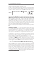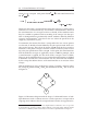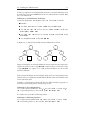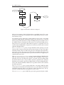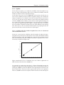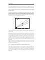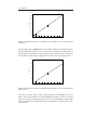
1
Aalborg University
The Faculty of Engineering and Science
Department of Computer Science
Fredrik Bajers Vej 7E
9220 Aalborg Øst
Denmark
R ELA XML
A Tool for Transferring Data between
Relational Databases and XML Files
Steffen Ulsø Knudsen
Christian Thomsen
Master’s Thesis, Spring 2004
e
Aalborg University
The Faculty of Engineering and Science
Department of Computer Science
Fredrik Bajers Vej 7E
9220 Aalborg Øst
Denmark
R ELA XML
A Tool for Transferring Data between
Relational Databases and XML Files
Steffen Ulsø Knudsen
Christian Thomsen
Master’s Thesis, Spring 2004
e
Aalborg University
The Faculty of Engineering and Science
Department of Computer Science
ABSTRACT
TITLE:
R ELA XML
– A Tool for Transferring Data between
Relational Databases and XML Files
PROJECT PERIOD:
DAT6,
February 2 - June 9, 2004
PROJECT GROUP:
G3-110
GROUP MEMBERS:
Steffen Ulsø Knudsen, [email protected]
Christian Thomsen, [email protected]
SUPERVISOR:
Kristian Torp, [email protected]
NUMBER OF COPIES:
NUMBER OF PAGES:
9
108
e
This report describes the platform independent tool R ELA XML that can be used for transferring data between relational databases and
XML files. The tool uses SAX technology and
is thus able to handle large files.
The format of the XML file generated by R E LA XML is specified by the user. Many formats
– also grouping of similar elements – are supported. Transformations, which should be applied to the data when exported, can be defined. For example, it is possible to encrypt
sensitive data or convert between units.
It is often required that the exported XML files
can be reimported into the relational database.
For instance, this is the case when the XML
files have been updated or if the data should be
imported into a new database. If some simple
conditions are fulfilled, R ELA XML is capable
of importing the data again.
When doing an export, R ELA XML gives guarantees about whether it is possible to import
the data again. Furthermore, R ELA XML offers
possibilities for deleting data in an XML document from the database.
When an updated XML document is imported,
R ELA XML ensures that occurrences of redundant data are updated consistently. The user is
allowed to update values in the XML and is not
required to provide explicit informations about
which values have been changed.
In the report, formal descriptions of the export and import operations are given. Further, design and implementation issues are described. A performance study shows good performance. The study shows that import and
export through R ELA XML have an overhead
of about 100% compared to direct use of SQL
through JDBC.
The main contributions of the report are the
guarantees on importability at export time and
the ability to make very powerful and flexible
transformations of the data both when exporting and importing.
Preface
This report is written in the spring 2004 by Group G3-110 as documentation
for the DAT6 project (Master’s Thesis) at the Database and Programming Technologies Research Group, Department of Computer Science, Aalborg University.
This project is based on the work described in our DAT5 report on the prototype of R ELA XML. The prototype had a code base of approximately 3,000 lines
of Java code but the code base has been completely rewritten to reflect the new
functionality described in this report. The new implementation of R ELA XML
consists of approximately 8,500 lines.
The project web site is available at
http://www.relaxml.com
The web site contains the source code and JavaDoc. Furthermore, the report
and the installation files are available for download.
Notation
In the report, names of classes, variables and methods are written in a mono
spaced font for easy identification. We sometimes refer to a W3C XML Schema by the notion Schema (with a capital S) whereas schema (with a lower case
s) just refers to a schema in general. References are given in square brackets
like [GHJV95].
Prerequisites
We assume that the reader has knowledge of object-oriented design, Java, JDBC
(especially the JDBC database metadata model), SQL, elementary graph theory
and XML. We also assume that the reader has a knowledge of relational algebra.
References may be found in the bibliography. For an introduction to the graph
theory [CO93, Ros95] are good sources. A thorough introduction to JDBC can
be found in [Ree00] and introductions to relational algebra can be found in
[SKS02, Dat00]. [Cel00] gives a thorough introduction to SQL and [Ray03] explains the basics of XML.
i
ii
License
R ELA XML is released as an Open Source tool under the Apache 2.0 License
which is available from http://www.apache.org/licenses/LICENSE-2.0.
Acknowledgements
We would like to thank Logimatic for their comments and Lyngsoe Systems for
providing data. We would also like to thank the Oticon Fonden for supporting
us financially.
Aalborg, June 2004
Steffen Ulsø Knudsen
Christian Thomsen
Contents
1 Introduction
1.1 General Problem . . .
1.2 Assumptions . . . . . .
1.3 Related Work . . . . .
1.4 Structure of the Report
.
.
.
.
1
1
3
3
4
2 Informal Description
2.1 Concepts . . . . . . . . . . . . . . . . . . . . . . . . . . . . . . . .
2.2 Structure Definitions . . . . . . . . . . . . . . . . . . . . . . . . .
2.3 Operations . . . . . . . . . . . . . . . . . . . . . . . . . . . . . . .
5
5
6
8
.
.
.
.
.
.
.
.
.
.
.
.
.
.
.
.
.
.
.
.
.
.
.
.
3 Formal Description
3.1 Transformations . . . . . . . . . .
3.2 A Formal Definition of Concepts
3.2.1 Basic Definition . . . . . .
3.2.2 Concept Inheritance . . .
3.3 Defining the XML Structure . . .
3.4 Creating the XML . . . . . . . . .
3.5 Importing the XML . . . . . . . .
3.6 Deleting Data From the Database
.
.
.
.
.
.
.
.
.
.
.
.
.
.
.
.
.
.
.
.
.
.
.
.
.
.
.
.
.
.
.
.
.
.
.
.
.
.
.
.
.
.
.
.
.
.
.
.
.
.
.
.
.
.
.
.
.
.
.
.
.
.
.
.
.
.
.
.
.
.
.
.
.
.
.
.
.
.
.
.
.
.
.
.
.
.
.
.
.
.
.
.
.
.
.
.
.
.
.
.
.
.
.
.
.
.
.
.
.
.
.
.
.
.
.
.
.
.
.
.
.
.
.
.
.
.
.
.
.
.
.
.
.
.
.
.
.
.
.
.
.
.
.
.
.
.
.
.
.
.
.
.
.
.
.
.
.
.
.
.
.
.
.
.
.
.
.
.
.
.
.
.
9
9
10
10
12
14
16
18
20
4 Design
4.1 Flow of Data . . . . . . . . . . . . . . . . . .
4.2 XML Parsing . . . . . . . . . . . . . . . . . .
4.3 Export . . . . . . . . . . . . . . . . . . . . .
4.3.1 Concepts and SQL Code Generation
4.3.2 Dead Links . . . . . . . . . . . . . .
4.3.3 XML Writing . . . . . . . . . . . . .
4.3.4 Generation of XML Schemas . . . .
4.4 Import . . . . . . . . . . . . . . . . . . . . .
4.4.1 Requirements for Importing . . . . .
4.4.2 Avoiding Inconsistent Updates . . .
4.4.3 Database Model . . . . . . . . . . . .
4.4.4 Execution Plan . . . . . . . . . . . .
4.4.5 Importing the Data . . . . . . . . . .
4.5 Delete . . . . . . . . . . . . . . . . . . . . . .
4.5.1 Requirements for Deletion . . . . . .
4.5.2 Inferring on the Database Schema .
.
.
.
.
.
.
.
.
.
.
.
.
.
.
.
.
.
.
.
.
.
.
.
.
.
.
.
.
.
.
.
.
.
.
.
.
.
.
.
.
.
.
.
.
.
.
.
.
.
.
.
.
.
.
.
.
.
.
.
.
.
.
.
.
.
.
.
.
.
.
.
.
.
.
.
.
.
.
.
.
.
.
.
.
.
.
.
.
.
.
.
.
.
.
.
.
.
.
.
.
.
.
.
.
.
.
.
.
.
.
.
.
.
.
.
.
.
.
.
.
.
.
.
.
.
.
.
.
.
.
.
.
.
.
.
.
.
.
.
.
.
.
.
.
.
.
.
.
.
.
.
.
.
.
.
.
.
.
.
.
.
.
.
.
.
.
.
.
.
.
.
.
.
.
.
.
.
.
.
.
.
.
.
.
.
.
.
.
.
.
.
.
23
23
24
26
26
28
31
32
34
34
36
37
39
42
45
45
46
iii
.
.
.
.
.
.
.
.
.
.
.
.
.
.
.
.
.
.
.
.
.
.
.
.
.
.
.
.
.
.
.
.
.
.
.
.
.
.
.
.
Contents
iv
4.5.3
4.5.4
4.5.5
Limitations . . . . . . . . . . . . . . . . . . . . . . . . . .
An Alternative Delete Operation . . . . . . . . . . . . . .
Solutions . . . . . . . . . . . . . . . . . . . . . . . . . . . .
50
51
52
5 Implementation
5.1 Packages of R ELA XML . . . . . .
5.2 Problems . . . . . . . . . . . . . .
5.3 Transformations and Data Rows
5.3.1 Scope of Columns . . . .
5.4 Implementation of Parsers . . . .
.
.
.
.
.
.
.
.
.
.
.
.
.
.
.
.
.
.
.
.
.
.
.
.
.
.
.
.
.
.
.
.
.
.
.
.
.
.
.
.
.
.
.
.
.
.
.
.
.
.
.
.
.
.
.
.
.
.
.
.
.
.
.
.
.
.
.
.
.
.
.
.
.
.
.
.
.
.
.
.
.
.
.
.
.
.
.
.
.
.
55
55
58
59
60
61
6 Performance Study
6.1 Test Setup . .
6.2 Start Up Costs
6.3 Export . . . .
6.4 Import . . . .
6.4.1 Insert .
6.4.2 Update
6.5 Delete . . . . .
6.6 Conclusion . .
.
.
.
.
.
.
.
.
.
.
.
.
.
.
.
.
.
.
.
.
.
.
.
.
.
.
.
.
.
.
.
.
.
.
.
.
.
.
.
.
.
.
.
.
.
.
.
.
.
.
.
.
.
.
.
.
.
.
.
.
.
.
.
.
.
.
.
.
.
.
.
.
.
.
.
.
.
.
.
.
.
.
.
.
.
.
.
.
.
.
.
.
.
.
.
.
.
.
.
.
.
.
.
.
.
.
.
.
.
.
.
.
.
.
.
.
.
.
.
.
.
.
.
.
.
.
.
.
.
.
.
.
.
.
.
.
.
.
.
.
.
.
.
.
63
63
63
64
69
69
72
74
76
7 Concluding Remarks
7.1 Future Work . . . . . . . . . . . . . . . . . . . . . . . . . . . . . .
77
79
A User Manual
A.1 Options XML Files . . . . . . .
A.2 Concept XML Files . . . . . . .
A.3 Structure Definition XML Files
A.4 Performing an Export . . . . . .
A.5 Performing an Import . . . . .
A.6 Performing a Deletion . . . . .
81
81
83
85
87
87
88
.
.
.
.
.
.
.
.
.
.
.
.
.
.
.
.
.
.
.
.
.
.
.
.
.
.
.
.
.
.
.
.
.
.
.
.
.
.
.
.
.
.
.
.
.
.
.
.
.
.
.
.
.
.
.
.
.
.
.
.
.
.
.
.
.
.
.
.
.
.
.
.
.
.
.
.
.
.
.
.
.
.
.
.
.
.
.
.
.
.
.
.
.
.
.
.
.
.
.
.
.
.
.
.
.
.
.
.
.
.
.
.
.
.
.
.
.
.
.
.
.
.
.
.
.
.
.
.
.
.
.
.
.
.
.
.
.
.
.
.
.
.
.
.
.
.
.
.
.
.
.
.
.
.
.
.
.
.
.
.
.
.
.
.
.
.
.
.
.
.
.
.
.
.
.
.
.
.
.
.
.
.
.
.
.
.
.
.
.
.
.
.
.
.
.
.
.
.
.
.
.
.
B Example
89
C XML Schemas for Setup Files
C.1 Options XML Schema . . . . . . . . . . . . . . . . . . . . . . . . .
C.2 Concept XML Schema . . . . . . . . . . . . . . . . . . . . . . . .
C.3 Structure Definition XML Schema . . . . . . . . . . . . . . . . . .
97
97
98
100
Bibliography
103
Summary
107
Chapter 1
Introduction
In this chapter, we introduce the problem of transferring data between relational databases and XML documents. It is a purpose of the tool R ELA XML,
described in this report, to perform such transfers. Whenever we use the term
database we assume that it is a relational database.
1.1 General Problem
It is often useful to be able to export data from a relational database to a vendorindependent format. This could be done to share the data with an external
partner, process the data in another dedicated application or to copy the data
to another database.
To be useful it should, however, also be possible for the tool to import data
back into the database (or to another database with a compatible schema). It
would then be possible for a company to export data of a purchase order and
send the exported document to a supplier. The supplier could then add information to the document about delivery dates and prices. When the company
then receives the updated document, the updated data could be imported into
the database again.
XML [W3Cb] is a widely used standard for exchanging data. XML is vendorindependent, flexible and has a clear semantics. Thus it is an obvious choice
as the external format. XML documents may be either document-centric or
data-centric. Document-centric documents are (usually) designed for human
consumption whereas data-centric documents are designed for data transport
[Bou03]. Since R ELA XML uses XML for transporting data between a database
and other applications, R ELA XML models the data using data-centric XML
documents.
The overall problem is shown in Figure 1.1 on the following page where data
from a database is exported as a set of XML documents. These XML documents
may be used by other applications (or tools). Once these applications have finished and maybe updated the XML documents, the changes can be propagated
back to the database.
1
Chapter 1. Introduction
2
XML
Export
Application
Database
Import
XML
(changed)
Figure 1.1: Pictorial view of the export and import procedures.
When data from a database is exported, there are several interesting problems
to consider. It should be considered which data to export. Typically, one would
only be interested in exporting a well-defined subset of the data, not the entire
database. To export the complete database might be easier than to define which
parts to export, but this could result in huge data sizes being exported. Furthermore, this might be forbidden by legal or business reasons. But when only
parts of the data are exported it might not be possible to propagate changes
back to the database again. This could happen if there is no way of uniquely
identifying the tuples to update in the database.
A second problem to consider, is whether it is possible to insert the data from
an XML document into another database that does not contain the data already.
Even if it is possible to propagate updates back to the database the data originated from, it might be impossible to insert the data into a compatible, empty
database. This situation could happen, for example, if an exported foreign key
is referencing something in the database that is not included in the exported
XML document.
A third problem to consider is whether it is possible to delete data by means
of an XML document such that R ELA XML automatically can delete the corresponding data from the database.
The report will deal with all of these problems along with a description of how
the tool R ELA XML is designed and works.
One should note that there are dedicated tools for dumping a complete database to files and that the purpose of R ELA XML is different from the purposes of
such tools.
When using some of the tools currently available the user must specify the
export and import in detail for every export and import. This can be rather
cumbersome and different to reuse. With R ELA XML the user should be able
to use predefined concepts and does not have to think about the database in-
1.2. Assumptions
3
ternals. When exporting data to XML with R ELA XML, the user must be given
warnings if the data cannot be imported again.
In order to map the data to an XML document, the user defines a tree structure
for the XML. Notice, that the goal is not to cover every possible XML schema.
We cover a large subset of schemas and if necessary a final conversion may be
achieved using, for example, XSLT [W3Cd] stylesheets or similar techniques.
Figure 1.2 shows the procedure when exporting data from a database to an
XML document. The import procedure is basically the reversed of the procedure shown in the figure. An export is specified using a concept and a structure
definition. These specify the data of the export and structure of the corresponding XML document, respectively. These notions are introduced in details later
in the report. From the concept, SQL that extracts the data is generated. This results in a derived table that might be changed by user-specified transformations.
The data in the resulting table is exported to XML with a schema as described
in the structure definition.
Concept
Structure
Definition
Database
Transformed
Derived Table
Derived Table
SQL
Transformations
XML Document
and Schema
<A>
<B>xyz</B>
</A>
<C>
<D>xyz</D>
<E>xyz</E>
</C>
Figure 1.2: An overview of the R ELA XML export procedure.
1.2 Assumptions
In this section, we present the overall assumptions taken in R ELA XML.
The tool R ELA XML should be DBMS independent and thus should not be tied
to any specific vendor’s product. Further, it should be able to cope with large
amounts of data. That is, we do not assume that R ELA XML will be able to hold
all the data of an export in main memory.
In addition, we assume that the data to extract from the database can be taken
directly from one table or from a join of two or more tables. It is assumed that
these tables are all from the same database schema.
1.3 Related Work
Many products that combine XML and database technology exist. There are
many DBMSs that are so-called XML-enabled databases, which means that they
are DBMSs with extensions for transferring data between XML documents and
4
Chapter 1. Introduction
themselves [Bou04]. The solutions available in such products are often vendor specific with SQL/XML [Gro03] as an important exception to this. A comparison of the XML support in the major commercial DBMSs can be found in
[CRZ03].
SQL/XML is a new standard for a set of XML extensions to SQL. [Tec03] shows
how the use of SQL/XML instead of non-portable proprietary solutions makes
the required code easier to write and maintain. A problem with SQL/XML is
that it, for the time being, only supports queries (i.e., export of data to XML)
and not updates (i.e., import of data from XML) [Tec03]. Therefore, other tools
are required to import data from XML.
There also exist many middleware products (such as R ELA XML). A middleware
product is a piece of software which is outside the DBMS and can be used to
transfer data between databases and XML documents. [Boub] maintains a thorough list of middleware products and descriptions of these. The list includes
both products that can either export or import and tools that can do both. A few
examples from the list are JDBC2XML [Res], DataDesk [Tec] and XML-DBMS
[Boua]. Of these examples, XML-DBMS is the most interesting since it is capable of both importing an exporting. It uses a mapping language to provide
flexible mappings between XML elements and database columns. The mappings can also be automatically generated from a DTD or database schema.
A tool which is not in [Boub] is PolarLake Database Integrator [Pol]. This is
a powerful tool which can do bidirectional mapping between XML elements
and columns in different tables in a database. Further, the tool supports userdefined transformations. The tool is commercial and there is little information
available on the details of the product.
1.4 Structure of the Report
In Chapter 2, we informally introduce the notions used in the report. The chapter is included to give the reader a sense of the notions before they are formally
defined in Chapter 3. In Chapter 4, we present the design of R ELA XML. This
includes descriptions of how to retrieve data from the database and how to create XML documents based on the data. Further, the requirements for being able
to import the data back to a database are described. Algorithms and methods
for importing data are also presented. Chapter 5 describes the most interesting
implementation issues and is followed by a performance study in Chapter 6.
Appendix A contains a user manual to R ELA XML. This is followed by a longer
example of export and import in Appendix B. Appendix C shows the XML
Schemas for the XML files required by R ELA XML for setup and usage.
Chapter 2
Informal Description
In this chapter, we give informal descriptions of the different notions used in
this report. The descriptions are at a high level of abstraction since they are
meant to provide an overview before the formal descriptions given in the next
chapter. All terms introduced in this chapter will be reintroduced in the next
chapter in a formal manner.
When data is to be exported by R ELA XML, the tool must know what data to
export and how to present it. For this concepts and structure definitions are used.
These are described in the following two sections.
2.1 Concepts
A concept defines the data to include in an export. Thus, a concept describes
the table columns included in an export and how the underlying tables are
joined. The data defined by a concept results in a table and has a flat structure.
Further, a row filter can be defined as part of a concept. This filter is used for
excluding rows which the user is not interested in. A concept must also hold
a caption. The caption is used as the name of the root element in the XML
document generated by R ELA XML.
Since two columns from different tables can have identical names a renaming
schema is applied when the data to export is retrieved. In the renaming the
column names are prefixed with the name of the base tables1 . This new name
is again prefixed with an encoding2 of the used concept. The latter is due to the
fact that concepts can be combined to form new concepts. This will be introduced shortly.
When data is exported it is possible to transform the data by applying a se1 From the point of view of R ELA XML there is no difference between a base relation and a view.
Thus the term base relation also includes views in the database. Note that the result of a concept is
not a base relation.
2 It is important that the encoding is unique. In the implementation this encoding is the filename of the concept XML file which can be chosen uniquely for each concept independently of its
caption.
5
6
Chapter 2. Informal Description
quence of transformations. For example, it is possible to encrypt data or to convert from one currency to another.
The data to export as defined by the concept is a set of tuples or rows. A transformation is a function that works on one row at a time and is capable of transforming the data in the row (i.e., update existing columns), add new columns,
or delete existing columns. Before the XML is generated each row can be transformed. It is specified in the concept which transformations to apply.
It is possible for a concept to inherit from another concept. A concept that inherits from another concept will include the data defined by the parent concept.
Transformations defined by a parent concept will be applied to the data of the
parent. In addition, the specialized concept can also transform the data of the
parent. It is possible to inherit from more than one parent. This is termed multiple inheritance.
Inheritance is the reason for the addition of information about the concept to all
column names in the renaming schema mentioned above. If two concepts include the same column, it will be added twice, but with different names. If this
was not the case, problems could emerge if a transformation included from one
concept would transform the data in the column, but the data already had been
transformed to an unexpected value (for example from decimal representation
to hexadecimal) by another concept that is not an ancestor of the first concept.
In the general case, the two concepts do not know of each other (a concept only
knows about its ancestors) and therefore we must ensure that each concept’s
transformations see the data as is expected from within their concepts.
2.2 Structure Definitions
The data defined by a concept has a flat form. To export the data to XML, a tree
structure for the data must be used. When XML is generated for some given
data, many formats or structures of the XML are possible in the general case.
A structure definition defines the structure of the XML that should hold the
data that a concept results in. By separating content (i.e., concept) and form
(i.e., structure definition), it is easy to export the same data to different XML
formats.
Basically, a structure definition maps the set of column names in the transformed derived table to element types or attribute types in the XML document.
For each of these element and attribute types, the structure definition states
which element type is its parent element type in the XML. A structure definition can only be used with a concept containing the columns that the structure
definition defines the position of in the XML. We say that a structure definition
complies with a concept if this is the case. A structure definition can also add
additional element types (called containers) that should not directly hold any
data from the concept, but only other elements. In this way, it is possible to
add an Address tag around Street and City tags, for example.
For a given structure definition and a set of rows resulting from a concept, R E LA XML iterates through the set of rows and writes XML tags corresponding
to the names and at the positions specified in the structure definition. Because
2.2. Structure Definitions
7
of the data-centric approach taken, an element either contains character data
or other elements – but not both. However, all the element types can have attributes.
It is possible to group by certain element types in the XML document. When this
is done similar elements of that type in the XML are coalesced. The elements
coalesced are those that have the same attribute values and content (disregarding the values of children elements). The children of a coalesced element are the
children of all the coalesced elements. It is, however, also possible to group by
the element type’s children element types, i.e., we can group on several levels
in the XML tree. In the following, we consider the same data presented when
we do not group by any element types and when we group by the element
types A and B.
Listing 2.1: XML excerpt representing the data set when the XML is not grouped
by any element types.
1 <Example>
2
<A value="1">
3
<B value="1">
4
<C>1</C>
5
</B>
6
</A>
7
<A value="1">
8
<B value="1">
9
<C>2</C>
10
</B>
11
</A>
12 </Example>
Listing 2.2: XML excerpt representing the data set when the XML is grouped
by element types A and B.
1 <Example>
2
<A value="1">
3
<B value="1">
4
<C>1</C>
5
<C>2</C>
6
</B>
7
</A>
8 </Example>
Note that in the first example there are two A elements that each contains one
B element. In the second example there is only one A element that contains one
B element. This B element, however, now holds two C elements.
In the following, we describe the requirements for grouping. Later, in Section 3.3, we describe the requirements in a more formal manner. It is not possible to group by a child without grouping by its parent. This it not possible
since there would not be any children to coalesce anyway (all element type
names are unique among siblings). Further, we require that there is at least one
of the element types in the XML that we do not group by. The reason for this
is that one row from the set of rows resulting from a concept should at least
generate one element in the XML such that it is possible to regenerate the rows
from the XML. If this is not the case, we cannot reconstruct all the data rows,
i.e., the grouping is lossy. These requirements are the core requirements. An
additional requirement is that if an element type x is followed by another element type y , which we group by in the XML, then we must also group by x. If
Chapter 2. Informal Description
8
we did not require this, we could not write the y elements before all rows had
been processed since we had to finish all x elements first. This would lead to
a much greater memory usage and we do not want to rely on holding all data
in memory as described in Section 1.2. However, the requirement does not impose any restrictions on the user’s final document, since all element types that
we group by could be placed such that they follow each other directly. When
the XML has been written, it is then possible to specify an XSLT transformation
that swaps two elements such that their positions are interchanged.
2.3 Operations
As previously described, it should be possible to transfer data between relational databases and XML files. Thus, it should be possible both to export from
and import to the database. When importing, there are multiple possibilities.
It is possible to insert such that the data in an XML file is copied into the
database3. It is also possible to update the data in the database. When this is
done, no tuples are added to the database. Instead, existing tuples are updated
such that some of their attributes are changed. It is also possible to merge. When
this is done, existing tuples are updated if their data has been changed in the
XML document. If new data has been added to the XML document, new tuples are added to the database. Further, it should be possible to delete data by
means of an XML document in the database. When this is done, tuples are
deleted from the databases.
The following chapter will present formal definitions of the mentioned operations.
3 In
R ELA XML this is done in such a way that the data is allowed to be in the database already.
Chapter 3
Formal Description
In this chapter, we give formal definitions of the material described in the previous chapter. First, we define transformations formally and then we define
concepts and structure definitions. Second, we present the structure and content of an XML document generated for a given concept and structure definition in a formal manner. Finally, we define the import and delete operations
supported by R ELA XML.
3.1 Transformations
In this section, we describe transformations which are used for transforming the
data when transferring data between the database and the XML documents.
Transformations consider rows. One row is transformed to exactly one other
row.
Formally we define a row to be a set of named attributes.
Definition 3.1 (Row)
A row is a finite set of components of the form a : v where it for a : v and
b : w is given that a = b ) v = w. For a component a : v, a is denoted as the
attribute name and v is denoted as the attribute value.
r = fa1 : v1 , : : : , an : vn g we let r[ai ℄ = vi , 1 i n and let
N (r) = fa1, : : : , ang. The set of all rows is denoted R.
For a row
We now define transformations. A transformation is a function that works on
rows.
Definition 3.2 (Transformation)
A transformation t is a function t : R ! R that fulfills N t(r) = N t(s) for
all r, s 2 dom(t) where dom(t) is the subset of R that rows to be transformed
by t must belong to.
This means that a transformation can add and remove attribute names. However, this must be done in a consistent manner such that all rows in the do9
Chapter 3. Formal Description
10
main of a transformation have identical sets of attribute names when transformed. Further, a transformation can change all attribute values. The set of
attribute names added by a transformation t is denoted (t), and the set of
names deleted by a transformation t is denoted Æ (t).
In some cases, we wish to ensure that a transformation does not change certain
attribute values. For this we use restricted transformations.
Definition 3.3 (Restricted Transformation)
The transformation t is a transformation restricted from C iff
8r 2 R : r[x℄ = t(r) [x℄
if x 2 C .
We say that t is a restricted transformation.
3.2 A Formal Definition of Concepts
In this section, we give a formal definition of concepts. A concept forms the
basis for an export in which the part of the database to be exported is defined.
Concepts may inherit from other concepts, as described in the following. Since
inheritance gives rise to special considerations we first present the basic definition and the interpretation of a concept that does not inherit from other concepts. Next, concept inheritance is described.
3.2.1 Basic Definition
A concept should present a well-defined part of the database to be exported.
When the data for the export is extracted the concept forms the basis for building the SQL statement retrieving the data, see Section 4.3.1.
We consider the set = I [ O where I = fg and O = fLOJ , ROJ , F OJ g 1
are the join operations supported by R ELA XML. Note that the operators from
O are neither commutative nor associative.
We now define a join tuple. This will be used later on for defining concepts
formally.
Definition 3.4 (Join Tuple)
A join tuple is a three-tuple of the form
((r1 , : : : , rm ), (!1 , : : : , !m 1), (p1 , : : : , pm 1)), m 1
where
ri is a relation or another join tuple for 1 i m
!i 2 for 1 i m 1
pi is a predicate for 1 i m 1.
1 Let
be a join, LOJ be a left outer join, ROJ be a right outer join and FOJ be a full outer join.
3.2. A Formal Definition of Concepts
Further, we require that if !i
11
2 O then !j 2 I for j < i.
For an ! 2 and a predicate p we let A ! p B denote the join (with type defined
by ! ) where the predicate p must be fulfilled. For a given join tuple r it is then
possible to compute a relation by means of the eval function which is given as
eval(r) =
8
>
>
<
>
>
:
eval(r1 ) !1p1 eval(r2 ) !2p2
!mp
m
1
1
eval(rm )
r
= ((r1 , : : : , rm ),
(!1, : : : , !m 1),
(p1, : : : , pm 1))
if r
if r is a relation.
That is, the value of eval applied to a relation is the relation itself. The value of
eval applied to a join tuple is the relation that arises when the values of eval
applied to the elements in the first component of the join tuple are joined. Note
that even though the operators in O are not associative nor commutative the
value of eval is unambiguously defined. The reason for this is that that we in
Definition 3.4 require that an operator from O cannot be followed by another
operator from O. If more than one operator from O must be used to compute
a relation, then this is modeled by inserting a join tuple with the first operator
from O into another join tuple with the second operator from O.
Note that a Cartesian product is modeled as a theta join with the join predicate
true.
Definition 3.5 (Concept)
A concept k is a 6-tuple (n, A, J , C , f , T ) where n is the caption of the concept,
A is a possibly empty sequence (without duplicates) of parent concepts which
the concept inherits from, J is a join tuple, C is a set of included columns from
the base relations of J , f is a predicate acting as a row filter and T is a possibly
empty sequence of transformations to be applied to the data during export.
The predicate of a row filter can be composed by other predicates using the
connectives and, or and not. A predicate can for example for a given row compare two columns or a column and a constant using =, 6=, <, , > or .
The relation valued function D computes the base data2 for a concept. For a
concept k = (nk , (a1 , : : : , am ), Jk , Ck , fk , Tk ), the function D is given as follows,
where for a column we let () denote the name of the table from which the
column originates and where ols(x) gives all the columns in the relation x.
D(k) = 2,C [hki# ()$/℄ (C [f~ j ~2ols(D(a )), i=1,:::,ng (f (eval(Jk ))))
k
k
i
k
(3.1)
Thus, first eval is used to compute the relation that holds the data from the
used base relations. Then a selection is performed on this relation before a projection of all columns included by k or any of its ancestors. Finally, a renaming
schema of the columns included by k is used by means of the rename operator where # and $ represent separator characters. This 3-part naming schema
(concept name, table name, column name) is necessary in order have a one-toone mapping from the columns of D(k ) to the columns of the database and to
2 By
base data we mean data that has not been transformed yet.
Chapter 3. Formal Description
12
handle scope of columns. With the renaming schema, table names are part of
the column names of D(k ). The column names also reveal the concept in which
they were defined. This is necessary in order to separate the scopes of different
concepts. We will describe this in Section 5.3.1.
As shown above, D(k ) denotes a relation with the data of the concept k before
the transformations are applied. For a concept k with transformations T =
(t1 , : : : , tn ) and parent list A = (), i.e. no parents, the resulting data is given by
the relation valued function R defined as follows.
R(k) =
[
d2D(k)
,
a2(([t2T (t))n([t2T Æ(t)))
[hki#a/a℄ tn Æ tn
1
Æ Æ t2 Æ t1 (d)
(3.2)
As seen the transformations are applied to each row of D(k ) before columns
added by the transformations are renamed. Note that columns added by concepts are renamed in (3.1) and that columns added by transformations are renamed in (3.2). Note also, that columns added by a transformation do not follow the 3-part naming scheme since they do not originate from any base table.
However, they will always have the concept as the first part.
For a concept k we refer to D(k ) as the derived table of k and we refer to R(k ) as
the transformed derived table.
One should note that it must be possible for D(k ) and R(k ) to contain duplicate tuples because this is allowed in SQL. In general, this is not possible in
relational algebra.
3.2.2 Concept Inheritance
As described in the previous section, a concept can inherit from (also called
extend) another concept. In this section, we describe how this works and what
the resulting data looks like.
Consider a concept
= (n, A , J, C , f, T)
where A
= (a1 , : : : , an), n 1.
For such a concept, we require that the first component of J contains D(ai )
for i = 1, 2, : : : , n. This means that the concept which extends the concepts
a1 , a2 , : : : , an must include information about how to join the data from these
concepts to its own.
The base data of a concept with jAj > 0 is computed with the relation valued
function D defined in (3.1). Note how the naming schema is applied to the
concept by applying D recursively on the parents before renaming the columns
added by the concept itself.
The relation valued function R is given by
R() =
[
d2D()
() d
,
(3.3)
3.2. A Formal Definition of Concepts
where for any concept
T = (t1k , : : : , tkp )
(k) =
k
13
with parent list
,
(ak1 , : : : , aku ) and transformation list
n2(([t2T (t))n([t2T Æ(t)))
[hki#n/n℄ tkp Æ Æ t1k
Æ
(aku ) Æ Æ (a1k ).
This means that when a concept inherits from other concepts, a parent’s transformations are evaluated before any of its children’s transformations. When all
the transformations of a concept have been evaluated, all the attribute names
they have added are prefixed with an encoding of the concept. It is then possible to distinguish between identically named attributes added by different
concepts’ transformations3 . Note that in the case where the parent list is the
empty list, (3.3) reduces to (3.2).
To summarize, this means that when a concept that has one or more parents
is evaluated, we find the relation defined by the join expression of which contains parent concepts. This is done by means of D() which involves recursive
inclusions of the parent concepts. Then the relations found are joined according to the join specifications in the concept . At this point, the transformations
from the different concepts are applied by means of R(). In principle, when
a transformation is applied, the data from all the concepts is thus available.
However, in the implementation we use restricted transformations as defined
in Definition 3.3 such that a transformation can only transform data included
by the concept that defines the use of the transformation or an ancestor of that
concept.
With the definition in (3.3) a problem may emerge. Consider a situation where
the concept 4 inherits from 2 and 3 that both inherit from 1 . This is shown
in Figure 3.1.
1
2
3
4
Figure 3.1: Inheritance diagram with the shape of a diamond because of multiple inheritance with a common ancestor. A circle represents a concept and an
outgoing arrow indicates that the concept inherits from the concept pointed to.
3 The reason for this setup is that we in the implementation would like to have a scope rules
for transformations. It is then possible to add an attribute even though another attribute with the
same name was added by another transformation. This will be explained further in Chapter 5.
Chapter 3. Formal Description
14
Now assume that 1 includes the column k . Then this column is accessible from
the transformations included from 1 , 2 , 3 and 4 . But then the first transformation included from 2 will expect that the data for column k is as it was after
the last transformation included by 1 . The same is expected by the first transformation included by 3 . But then we do not have an order for how to apply
the transformations. Instead of defining complicated rules for how to handle
this situation, we choose to disallow a situation where a “diamond” as shown
in Figure 3.1 emerges. Thus, for any concept (n, A, J , C , f , T ) we require that no
concept is inherited from twice when the concepts in A and their parents, and
the parents’ parents and so on are included. Formally, we require that the list of
ancestor concepts (A) does not contain any duplicates where is recursively
defined as
(a1 :: :: an ) = a1 :: :: an :: p(a1) :: :: p(an )
(3.4)
and where p(x) is the list of parents from the concept x.
3.3 Defining the XML Structure
In Section 3.2, we introduced concepts which define the data for an export.
We now introduce structure definitions which define how the data of a concept
should be presented as an XML tree. Furthermore, grouping4 is defined in order
to allow grouping in XML documents.
Definition 3.6 (Structure Definition)
A structure definition S = (Vd , Vs , E ) is an oriented, ordered tree where Vs \
Vd = ; and V = Vs [ Vd is the set of vertices and E is the set of edges. A vertex
v 2 V is a tuple (, t, g) where is a name, t 2 felement, attributeg is the type
and g 2 ftrue, falseg shows if the XML data is grouped on the vertex. The
root = (, element, true) 2 Vs and for every v = (, t, g ) 2 Vs it holds that
t = element. For v = (, t, g) 2 Vd it holds that if t = attribute then v has
no children whereas if t = element then for each child (d, u, h) of v we have
u = attribute.
We say that a structure definition S = (Vd , Vs , E ) complies with a concept k
iff for each column of R(k ) there exists exactly one node in Vd with identical
name and the name of the root of S equals the caption of the concept k . For a
concept k a vertex v 2 Vd represents a column of R(k ) and will thus give rise
to elements that hold data. A vertex in Vs on the other hand does not represent
a column and will give rise to structural elements that hold other elements.
Since the XML structure is ordered, an order on the tree showing the ordering
of children elements exists.
For the vertices in a structure definition we let the function be a mapping between the names of the vertices and XML tag names. Thus, the XML elements
represented by v in the structure definition will be named (v ).
4 Note
that in some literature grouping is denoted as nesting.
3.3. Defining the XML Structure
15
In order to represent a meaningful XML structure a structure definition must
be valid. For a vertex v let De(v ) denote the set of descendants of v and Ch(v )
the set of children of v .
Definition 3.7 (Valid Structure Definition)
A structure definition S = (Vd , Vs , E ) with root and order o is valid iff
o() = 0
For all v 2 (Vd [ Vs ) we for all 2 De(v) have that o() > o(v)
For all a, b 2 (Vd [ Vs ) we have that for all a 2 De(a) it holds that
o(a) < o(b) ) o(a ) < o(b)
For all v 2 (Vd [ Vs ) there do not exist , d 2 Ch(v) such that =
6 d and
() = (d)
For all (, t, g ) 2 Ch() we have t = element.
In Figure 3.2, a valid and an invalid structure definition are shown.
A
A
0
0
B
E
B
B
1
4
3
4
C
D
F
C
D
E
2
3
5
1
2
5
(a)
(b)
Figure 3.2: Examples of structure definitions. A letter represents the name and a
number the order. A node of type element is represented as a circle and a node
of type attribute as a square. (a) A valid structure definition. (b) An invalid
structure definition.
In the structure definition shown in Figure 3.2(b), there are some problems: The
element A has two children named B, and the B with order 3 has children with
lower order than itself.
To define a valid grouping which tells how the XML should be grouped, we
need the terms preceding relative and following relative.
Definition 3.8 (Preceding Relative)
For a valid structure definition S = (Vd , Vs , E ) with order o, a vertex p
Vs ) is a preceding relative to the vertex v 2 (Vd [ Vs ) if o(p) < o(v).
2 (Vd [
In a similar way we define a following relative.
Definition 3.9 (Following Relative)
For a valid structure definition S = (Vd , Vs , E ) with order o, a vertex f
Vs ) is a following relative to the vertex v 2 (Vd [ Vs ) if o(f ) > o(v).
2 (Vd [
Chapter 3. Formal Description
16
We are now ready to define a valid grouping.
Definition 3.10 (Valid Grouping)
A valid grouping is a valid structure definition S = (Vd , Vs , E ) where for v
(n, t, g) 2 (Vd [ Vs ) where g = true the following holds.
=
For all preceding relatives (a, b, ) of v , we have = true.
For all children (a, b, ) of v where b = attribute it also holds that = true.
A following relative (a, b, ) of v exists such that = false.
If a following relative (a, b, ) where = false that is not a descendant of
v exists, then for all descendants (d, e, f ) of v it holds that f = true.
Please refer to the text following Listing 2.2 on page 7 for a discussion on the
requirements for a valid grouping.
Consider again Figure 3.2(a). Now assume that we group by E. Then to have a
valid grouping we must also group by A, B, C and D, but not by F.
3.4 Creating the XML
In this section, we define the function XML that, given a concept and a valid
grouping, computes XML that contains the data that R() computes.
The function XML uses the two auxiliary functions Element, which adds an
element tag, and Content, which adds the content of an element. These two
functions depend on the structure definition used and therefore when we use
them a subscript shows which structure definition to use. That is, for a structure
definition d we write Elementd .
In the following, we consider the concept with caption n and the valid grouping d = (Vd , Vs , E ) that has the root , complies with and has order o. One
should note that some of the symbols used are used both as XML symbols and
mere mathematical symbols. Therefore any symbol or string that is added to
the XML is written in another font. Further a white space that is added to
the XML is written as an underscore (_).
The function XML is defined as
XML(, d) =
<n_concept="hi"_structure="hdi">
Contentd (, R())
(3.5)
</n>
Thus, the function XML adds the root element of the XML. This XML element
is named after the caption of the concept . Further, informations about the concept and structure definition are added. Notice that the attributes “concept”
and “structure” are always added and are not represented in the structure definition. The children elements of the root element are then computed by the
function Contentd which uses the function Elementd .
3.4. Creating the XML
17
In the following, for a vertex v = (x, y , z ) in the structure definition, we let
v1 = x, that is, v1 denotes the first component of v. Further, we let Att(v) denote
the ordered (possibly empty) list of attribute children of v . Then for v with
Att(v) = (a1 , : : : , an) we define v as
v =
(v1 , a11, : : : , a1n)
(a11 , : : : , a1n)
if v
if v
2 Vd
2 Vs
(3.6)
That is, if v is a node in Vd , then v is the list of the names of v and all its attribute
children. If v is in Vs , then v is the list of all v ’s attribute children’s names.
Elementd is defined as
Elementd(v, P ) =
,
<(v 1 )_(a11 )="r[a1 ℄"_ : : : _(a1n )="r[an ℄">
8r2 (P )
v
Contentd (v, v=r (P ))</(v1 )>
(3.7)
for a relation P and a vertex v with attribute children fa1 , : : : , an g where ai
has lower order than aj for i < j . Note that the symbol Æ here denotes string
concatenation.
We now define the function Contentd . For a v = (k , t, g ) the definition of
Contentd depends on whether v 2 Vs or v 2 Vd and when v 2 Vs Contentd
also depends on the value of g (i.e., whether we group by the node or not). We
first consider the cases when v 2 Vs .
When we group by v redundant element children of
This is reflected in the following definition.
v should not be added.
Contentd (v, P ) =
,
Elementd e1 , e1 =w1 (P )
8w1:w1 21 (P )
,
e
8w2:(w1 ::w2)21 ,2 (P )
e
..
.
e
,
,
h
e
:::,
eh
e1 =w1 ,:::,eh =wh (P )
8r2
8w :(w1::::w )21 ,
h
Elementd e2 , e1 =w1,e2 =w2 (P )
(P )
Elementd eh , e1 =w1,:::,e =w (P )
h
h
Elementd(eh+1 , frg) Elementd(em , frg)
if v
2 Vs and g = true,
(3.8)
where
Ch(v) = fe1 , : : : , em g,
o(ei ) < o(ej ) for i < j ,
(x, y, z ) 2 fe1, : : : , ehg ) z = true
Chapter 3. Formal Description
18
and
(x, y, z ) 2 feh+1, : : : , em g ) z = false
(that is, we group by the children e1 , : : : , eh ) hold.
This shows that when we group by the children e1 , : : : , eh , for each distinct
value of the attributes in P that are represented by e1 (and its attribute children), we create an XML element. Inside this XML element, data or other elements are added recursively by means of Elementd which itself uses Contentd .
After each of these elements for e1 other elements are added for those attributes
that are represented by e2 (and its attribute children). But here we have to ensure that the values for e1 match such that we correctly group by e1 . After the
elements for e2 follow elements for e3 and so on until elements for all nodes
that we group by have been added. Then elements for those nodes that we do
not group by are added. Notice that for these nodes exactly one tuple is used
for each application of Elementd .
When Contentd is used on nodes that we do not group by, it is only given one
tuple at the time. The definition of Contentd is then
Contentd (v, frg) = Elementd(e1 , frg) Elementd(em , frg)
if v 2 Vs and g = false,
where
and
(3.9)
Ch(v) = fe1, : : : , em g
o(ei ) < o(ej ) for i < j .
That is, when we do not group by v
element child of v .
2 Vs we simply add one element for each
Now, we have to define Contentd for nodes in Vd . But from (3.7) and (3.8) we
have that whenever Contentd is given a node v 2 Vd , the given data has exactly
one value for the attribute that v represents. Thus, all that Contentd should do
is to add this value.
Contentd (v, P ) =
Contentd v , v (P )
Contentd v, frg = r[v℄
if jP j > 1 and v
if v 2 Vd .
2 Vd
(3.10)
3.5 Importing the XML
In the previous section we defined how to create the XML when the data is
present in the database. Sometimes an inverse operation is necessary. For example, this is the case when an empty database should be loaded with the
data in the XML file or when the data in the XML has been updated and the
changes should be propagated back to the database. We therefore introduce
what it means to import the XML. However, we distinguish between inserting
and updating from the XML.
In the following definitions we refer to different states of the database. The
value of the function D from (3.1) depends on the state of the database and we
3.5. Importing the XML
19
therefore refer to the value of D() in the specific state s as Ds (). Now consider
an XML document X created by means of the concept . By DXML (X ) we
denote the table with column names as D() and that holds exactly the values
resulting when the inverse transformations from have been applied to the
data in X . Thus it is a requirement for importing X that the transformations
of are inversible. In the following definitions we do not consider the possible
impacts of triggers.
We now give the definition of inserting from the XML.
Definition 3.11 (Inserting from XML)
For a given database inserting from the XML document
X =
<n_concept="hi"_structure="hsi">
</n>,
is to bring the database that holds the relations used by from a valid state a to
a valid state b where Db () = Da () [ DXML (X ) such that the only difference
between a and b is that some tuples may have been added to relations used by
.
This means that after the insertion the data in DXML is also present in the
database. The data in DXML or some of it can be in the database before the
insertion but only in such a way that no updates are necessary, i.e., data is only
added to the database, not changed in the database. After the insertion, the
database must still be in a valid state such that primary key values are unique
and so on.
We now proceed to the definition of updating from the XML.
Definition 3.12 (Updating from XML)
Consider the XML document
X =
<n_concept="hi"_structure="hsi">
</n>,
and assume that k is the set of renamed5 primary keys in the relations used by
.
For a given database that holds the relations used by and tuples such that
k (DXML (X )) k (Da ()), updating from the XML document X is then, by
only updating tuples in base relations used by , to bring the database from a
valid state a to a valid state b where for any tuple t
t 2 DXML (X ) ) t 2 Db (),
t 2 Da () ^ k (ftg) * k DXML (X )
and
5 Renamed
) t 2 Db ()
t 62 DXML (X ) ^ t 62 Da () ) t 62 Db ().
to comply with the three-part naming schema used in the derived table.
Chapter 3. Formal Description
20
Thus, when the data is updated, it is a requirement that for each tuple t in
DXML (X ) there is a tuple t0 with identical values for k in Da (). t0 will then be
replaced by t in the state b. The remaining tuples in state b are those tuples for
which no tuples in DXML (X ) have identical values for k .
It is, however, possible to combine inserting and updating to merging such that
either a tuple from the XML updates a tuple in the database or is added. This
is reflected in the following definition.
Definition 3.13 (Merging from XML)
Consider the XML document
X =
<n_concept="hi"_structure="hsi">
</n>,
and assume that k is the set of renamed primary keys in the relations used by
.
For a given database that holds the relations used by merging from the XML
document X is then, by only adding tuples to or updating tuples in base relations used by , to bring the database from a valid state a to a valid state b
where for any tuple t
t 2 DXML (X ) ) t 2 Db (),
t 2 Da () ^ k (ftg) * k DXML (X )
and
) t 2 Db ()
t 62 DXML (X ) ^ t 62 Da () ) t 62 Db ().
Notice that the requirement k (DXML (X )) k (Da ()) from Definition 3.12
is not present in Definition 3.13. In Definition 3.13 it is implied by t 2 DXML (X )
) t 2 Db () that a tuple in the database in state a for which a tuple t with
matching values for the primary keys exists in DXML (X ) is replaced in the
state b by t.
We will have more to say about importing in Section 4.4.1 where we consider
some additional practical requirements for importing data.
3.6 Deleting Data From the Database
In this section, we consider how to make it possible to delete tuples from the
database by means of XML documents. To delete, we use a delete document
which has the same structure as XML documents generated by R ELA XML,
i.e., the structure described in Section 3.4. As many as possible of the tuples
in the database with data present in the delete document will be deleted. The
reason that everything is not always removed, is that foreign key constraints
may forbid this.
Since delete documents must have the same structure as the XML documents
being exported/imported by R ELA XML. Then DXML can be computed for
3.6. Deleting Data From the Database
21
identification of the data to delete from the base relations. We are now ready to
proceed to give a definition of what it means to delete from the database using
a delete document.
Definition 3.14 (Deleting Base Data by Means of XML)
For a given database deleting base data by means of the XML document
X =
<n_concept="hi"_structure="hsi">
</n>,
is to bring the database that holds the relations used by the concept from a
valid state a to a valid state b. This should be done by deleting as few tuples
as possible from the base relations used by and without violating the foreign
key constraints of the database. It should hold that t 2 DXML () ) t 62 Db ()
unless some value in t is referenced by a foreign key in a tuple not (partly)
included by and in a relation that has not been declared to set the foreign
keys to a null or default value or delete referencing tuples if t is deleted.
The deletion of tuples from relations used by may lead to updates or deletion
of tuples of other relations in the database according to the integrity constraints
defined on the database. Apart from this, only tuples in relations used by will
be deleted.
An alternative for delete documents that explicitly state what to delete would
be to use implicit deletes. In this way data that has been deleted from an XML
document should be deleted from the database when the XML document is
processed. However, this has some serious drawbacks. The first problem is that
an empty (in the sense that only the root element is present) XML document
could result in the entire database being deleted. A second problem is that it
can be expensive to find the data that is not in the XML document, but would
be if the export was performed now. Another result would be that data, which
was added after the export was performed, would be deleted when the created XML was processed. For these reasons we do not want to rely on implicit
deletes.
Chapter 4
Design
In the last chapter, we formally described how to create XML by exporting
data by means of concepts and structure definitions and how to import the
data again. Based on the formal descriptions in that chapter, we now proceed
to describe the design of R ELA XML.
Important design criteria are to be platform and DBMS independent. These
criteria are met by using Java and JDBC.
4.1 Flow of Data
In this section, we sketch the flow of data in R ELA XML. The flow for an export
is shown in Figure 4.1 on the next page and explained below.
When an export is performed, a single SQL query is generated for the concept.
This query selects the data from the database. When the query is sent to the
DBMS through the JDBC API a ResultSet is returned. Note that at this point
we still have a tabular view on the data. A ResultSet iterator is then used for
reading the data from a result set and generating data rows that hold the data
from the result of the query.
The data rows are then sent through the sequence of transformations specified
by the concept one at a time. As shown in Figure 4.1, it is possible to add a
transformation after another transformation and thus apply the decorator pattern [GHJV95].
After the transformations, the data rows are sent to a sorting iterator if any
grouping should be used in the XML. The reason for this is that to be able to
place the correct elements in the XML output, the writer should see the data
rows in a sorted order (this is explained further in Section 4.3.3). To ensure that
the rows are sorted it, is not enough to make the result of the SQL query sorted
since the transformations may change the values of the data rows. Therefore,
the rows should be sorted after the last transformation. But since there might
be too many rows for handling the sort in main memory, the sorting iterator
places the rows temporarily in the database. When the last row from the orig23
Chapter 4. Design
24
Relational database
Concept
Data
ResultSet
Data
Sorting iterator
ResultSet iterator
Data row
Transformation1
Data row
Database
Data row
XML writer
Structure definition
XML elements
XML document
Data row
Transformationn
Data row
Figure 4.1: The flow of data in an export.
inal ResultSet has been transformed, it is possible to retrieve all the transformed rows again in a sorted order. For this, the sorting iterator is used. After
the sorting iterator, the rows are sent to the XML writer a row at a time.
If no sorting is required, i.e., if no grouping is used, a sorting iterator is not
used. In this case, the data rows are just sent directly to the XML writer.
The XML writer generates the resulting XML by means of the data rows and a
structure definition. This is described in Section 4.3.3.
When importing, the flow is basically reversed, see Figure 4.2 on the facing
page. As the XML document is read data rows are generated. These data rows
are transformed using the inverse transformations. The inverse transformations are applied in the inverse order of how their corresponding transformations are applied when exporting. The data rows are then handed to an Importer that constructs SQL INSERT and UPDATE statements which are sent
to the database.
When deleting, the flow is the same as when importing. The only difference is
that the data rows will be given to a Deleter that will construct SQL statements that delete the corresponding tuples from the database, if possible.
4.2 XML Parsing
In this section we list the XML parsers that R ELA XML uses. Concepts, structure definitions and options are all specified using XML files. During parsing
it is validated that the setup XML files conform to the XML Schemas in Appendix C.
4.2. XML Parsing
25
XML document
Structure definition
XML elements
XML reader
Data row
Transformation−1
n
Data row
Importer
Concept
Data
Relational database
Data row
Transformation−1
1
Data row
Figure 4.2: The flow of data in an import.
We have four parsers which all inherit from a standard parser. The eventbased parser technology SAX (Simple API for XML) [Bro] is chosen to minimize memory usage.
An alternative parser technology, which could have been used, is the DOM
(Document Object Model) technology [W3Ca]. SAX parsers have a constant
memory usage while the memory usage of DOM parsers grows with the size of
the XML documents. Furthermore, SAX parsers are faster than DOM parsers.
SAX parsers are event based which limits the parser to sequential access. In
contrast to this, DOM builds a complete tree in memory which can be accessed
randomly [Ray03, W3Ca].
The ConceptXMLParser parses concept XML files. When parsing, it sets the
caption of the concept, recursively parses parent concepts, sets up a join tuple,
included columns and a row filter. The parser also instantiates the transformations of the concept. The parser also checks that no multiple inheritance with
diamond shape or circular inheritance is present since this is not supported, as
explained in Section 3.2.2.
The StructureDefintionParser parses structure definition XML files. The
XML files hold information on the encoding and the mapping of null values.
Primarily, however, the XML files specify a structure for the resulting XML
document. Based on the concept and the structure specified in the structure
definition, it is possible to generate an XML Schema for the resulting XML document. The structure definition XML file also specifies whether such a Schema
should be generated.
The OptionsParser parses options XML files. An options XML file holds
among others informations about which driver to use, the URL of the database
and which temporary tables to use (their use will be described later). The options here are thus those that are specific for a site or user.
The XMLDataParser parses XML files previously generated by R ELA XML.
Chapter 4. Design
26
From the XML the parser creates data rows and hands them on to the Importer.
Every parser of R ELA XML inherits from StandardParser which holds common functionality of parsers used in R ELA XML.
4.3 Export
4.3.1 Concepts and SQL Code Generation
In this section, we describe the class Concept. The Concept class holds a
representation of the concept and provides a method for generation of SQL
code for retrieval of the data of the concept.
The concept specifies the data for the export using a join tuple which models
an SQL statement. The join tuple is modeled as a tree of DataNodes. A DataNode can either be a RelationNode, which just holds a relation represented
by a DataNode object, a BaseRelNode, which holds the name of the base
relation it represents, a ConceptRelNode, which holds the name of a parent
concept, or a JoinRelNode which specifies the join between two RelationNodes. The UML class diagram for the DataNodes is shown in Figure 4.3.
DataNode
+getBaseTableNames(): String[]
+generateSQLPart(hm:HashMap): String
+getConceptNames(): String[]
+getJoins(al:ArrayList): ArrayList
RelationNode
#content: DataNode
+addRelation(): void
BaseRelNode
#tableName: String
ConceptRelNode
#conceptName: String
JoinRelNode
-type: int
-column1: String
-operator: int
-column2: String
-relation1: RelationNode
-relation2: RelationNode
+addRelation(): void
Figure 4.3: UML class diagram of the DataNode classes
An assumption for R ELA XML is that tables used by concepts are combined
using join operations. The set operations and aggregate functions are not supported. The SQL queries constructed do never contain GROUP BY, ORDER BY
or HAVING clauses.
Basically the SQL statement for retrieval of data of a concept has three parts.
SELECT columns with renaming
FROM join tuple
WHERE row filter
(1)
(2)
(3)
In the first part, we impose the three-part naming schema, in the second part,
we specify the base relations and concepts from which the data originates and
how the data is extracted, and in the third part, we restrict the data using the
4.3. Export
27
row filter of the concept. Concepts may inherit from other concepts which are
used in the join tuple of the concept. The SQL statements for parent concepts
are included as nested SQL statements in the FROM part of the SQL statement.
Note that because of inheritance the actual columns and row filter of the concept consist of the columns and row filters of parent concepts together with
included columns and row filter defined in the concept itself.
Part 1 and part 3 may be generated by the Concept by looking at the inherited
columns (which at this point already follow the three-part naming schema),
its own columns and the row filter of the concept. Part 2 is generated by descending recursively into the join tuple where a RelationNode does not add
any SQL code, a BaseRelNode simply inserts the name of the base relation,
a ConceptRelNode invokes the generateSQL() method of the concept in
the node. And a JoinRelNode generates an SQL part for a join between two
relations (i.e., two RelationNodes) which we recursively descend1 .
Example 4.1
Given a database with the following relations R1 = (A, B ) and R2 = (A, B )
where we ignore types. Assume that the two separators in the naming schema
are # and $. Consider the following concepts which are given using the notation
from Section 3.2.
C 1 =(onept1, (), ((R1), (), ()), fR1.A, R1.B g, (C 1#R1$A < 5), ())
C 2 =(onept2, (C 1),
((C 1, R2), (), (C 2#R2$B = C 1#R1$A)),
fR2.A, R2.B g, (), ())
The SQL queries for the retrieval of the data of concepts
follows.
C1
and
C2
are as
Listing 4.1: SQL query for retrieving data of concept C 1
1 (SELECT
2
R1.A AS C1#R1$A,
3
R1.B AS C1#R1$B
4 FROM
5
R1
6 WHERE
7
(C1#R1$A < 5))
Listing 4.2: SQL query for retrieving data of concept C 2
1 (SELECT
2
C1#R1$A,
3
C1#R1$B,
4
R2.A AS C2#R2$A,
5
R2.B AS C2#R2$B
6 FROM
7
(SELECT
8
R1.A AS C1#R1$A,
9
R1.B AS C1#R1$B
10
FROM
11
R1
12
WHERE
13
(C1#R1$A < 5))
1 Recall that R ELA XML supports Cartesian products, -joins, full outer joins, left outer joins and
right outer joins. In the join predicate the operators =, <, >, , and = are supported.
6
Chapter 4. Design
28
14
15
16
17
JOIN
R2
ON
(C2#R2$B = C1#R1$A))
4
Note how the three-part naming schema is imposed and how the SQL code of
parent concepts appears as nested sub-queries. The code generation shown in
Example 4.1 generalizes to situations with multiple inheritance.
For a concept k , the SQL code computes the relation D(k ) defined in (3.1) on
page 11. When the data has been retrieved, the transformations of k are used for
computing the relation R(k ) defined in Section 3.2. A Concept object exposes
its transformations with the getTransformationsClosure() which gives
the transformations in the order they should be applied. The Concept class
also provides getDataRowTemplate() for exposing the resulting columns
and their types. This is used when generating an XML Schema for the resulting
XML document.
4.3.2 Dead Links
When exporting a part of the database, we may risk that the data is not selfcontained. If an element represents a foreign key column in the database we
may have a situation where an element holds data which is a reference to some
data not included in the export. We refer to such a situation as the referencing
element having a dead link.
Figure 4.4 shows two schemas which may lead to dead links when the data is
exported.
Employees
Departments
Employees
EmpID
DepartmentID
EmpID
Name
Name
DepartmentID
ManagerID
Name
ManagerID
(a)
(b)
Figure 4.4: Two schemas which may lead to dead links in an export. An arrow
shows a foreign key integrity constraint of the database schema.
Consider the data sets in Figure 4.5 which show examples of data from the
schema in Figure 4.4(a). The first data set does not have dead links while the
second has dead links.
4.3. Export
EmpID
1
2
3
29
Name
A
B
C
(a)
ManagerID
null
1
1
EmpID
2
3
Name
B
C
ManagerID
1
1
(b)
Figure 4.5: Two examples of data sets originating from the database schema in
Figure 4.4(a). The data in (a) does not have a dead link while the data in (b) has
two dead links since both tuples refer EmpID 1 which is not included in the
data set.
A dead link does not limit the possibility of updates during import assuming
that the element referenced in the dead link still exists in the database. Insertion into a new database is limited by a dead link since we get a foreign key
constraint violation in the database if the element referenced in the dead link
is not present in the database prior to the insertion.
Detection
In the following, we give an algorithm for detecting dead links in an export. Let
SD be the SELECT statement for the derived table and let DT be the derived
table returned when invoking SD . In order to find dead links we can invoke
the following algorithm.
Algorithm 4.1 Find dead links
Requires: The derived table DT
Ensures: The dead links in the derived table are returned
1:
2:
3:
4:
5:
6:
7:
8:
function F IND D EAD L INKS(DT )
for each table T contributing to the derived table DT do
Find the sequence A = (a1 , : : : , an ) of foreign keys in T also included
in DT
Find the corresponding sequence B = ((b1,1 , : : : , b1,m1 ), : : : , (bn,1 , : : : ,
bn,mn )) of candidate keys that are referenced by the foreign keys
in A where B is also in DT
for each ai 2 A do
M SELECT DISTINCT ai FROM DT WHERE NOT EXISTS
(SELECT B FROM DT WHERE ai = bi,1 OR . . . OR ai =
bi,mi )
result[T ℄[ai℄
return result
M
The user may then be warned of the existence of dead links if the result of
FindDeadLinks() is non-empty. Note that line 4 reflects that a candidate key
referenced by a foreign key may be included many times (but perhaps different inclusions hold data from different tuples in the database). To avoid a dead
link, it is enough that the referenced value is present somewhere in the referenced columns.
Chapter 4. Design
30
Resolution
When resolving the dead links, the goal is to expand the selection criteria such
that the missing tuples are added. This is done by expanding the WHERE
clause of the SQL statement by adding an OR clause with a condition selecting
the new tuples.
Note that the SQL statement consists of possibly many nested SELECT statements in the FROM clause and that because of the scope rules specialized concepts may include a WHERE clause conditioning on the columns of ancestor
concepts. For this reason, an expansion of the condition must in some cases be
added several places in the SQL.
Instead of the SQL statement described in Section 4.3.1, we move the WHERE
clauses of the nested queries to the outermost query where they are AND’ed
together as follows.
SELECT columns with renaming
(1)
FROM join tuple
(2)
WHERE row filters of all included concepts (3)
This means that the SQL statements in part 2 do not contain the WHERE clauses.
Even though SQL is a declarative language and that the semantics of the two
approaches are the same, the approach taken in Section 4.3.1 is optimized such
that conditions are applied as soon as possible which in most cases reduces
the cost of join operations[SKS02]. It is doubtable that all DBMS optimizers can
move all the conditions to the nested SQL statements when using the new approach. For this reason, we keep the approach in Section 4.3.1 as the default
structure of the SQL statement. If the user requests dead link resolution, we
use the statement described above.
The Concept class provides the method generateDeadLinkSQL() which
can be implemented similarly to generateSQL() (described in Section 4.3.1)
which, given an expansion, generates SQL of the form shown above.
The pseudo code for an algorithm that expands the selection criteria, such that
dead links are avoided, is shown in Algorithm 4.2.
Algorithm 4.2 Expand selection criteria to a fix point such that the derived
table has no dead links
Requires: The concept on and the initial criteria Ensures: New criteria where the dead links are resolved
1:
2:
3:
4:
5:
6:
7:
8:
function E XPAND _ REC(on, )
GenerateDeadLinkSQL(on) expanded with OR clauses in the criteria determine the derived table DT from DerivedSQL
DerivedSQL
deadlinks = findDeadLinks(DT )
for each deadlinks[t℄ do
for each deadlinks[t℄[a℄ do
for each value v in deadlinks[t℄[a℄ do
expand with “OR a = v ”
4.3. Export
9:
10:
11:
12:
31
if has been expanded then
return expand_re(on, )
else
return The algorithm terminates when no dead links are found thereby implying that
a fix point is reached. The resulting derived table for a concept on may then
be retrieved by the SQL statement GenerateDeadLinkSQL(con) expanded by
an OR clause with Expand_rec(con, "").
The crucial step of Algorithm 4.2 is the step in line 8 where the condition is
expanded. Because the size of the SQL statement is limited the expanded condition may lead to a SQL statement that is too large. In Algorithm 4.2 the expanding condition is expanded for every missing value. If we assume that the
values selected in the condition are taken from an ordinal type with an associated order, we could have used intervals to specify the values. This may lead to
a considerably smaller condition expansion and more efficient SQL statements.
4.3.3 XML Writing
Following the program flow described in Section 4.1, the data of the concept
is retrieved, transformed and written to an XML document. In this section, we
give a high-level description of how to write the XML.
A design criterion is that we do not want to rely on having all data stored in
memory at one time. For this reason, the algorithm for writing the XML works
such that whenever it gets a new data row, it will write out some of the data
to the XML. If grouping is not used, all the data represented in a data row will
be written to the XML when a data row is received. This is not necessarily the
case if grouping is used. Then, some of the data might already be present in
the current context in the XML and should thus not be repeated. To ensure
this, the algorithm considers data from two rows, namely the new row to write
out to the XML and the last row that was written to the XML. Therefore, the
algorithm never holds data from more than two rows. Thus, this is different
from the DOM approach where a tree representing the entire document and its
data is build in main memory before it is written to a file.
When grouping is used, it is a precondition for the algorithm that the data rows
are sorted by the columns corresponding to the nodes that we group by. When
we group by more than one node, we should first sort by columns corresponding to nodes with lower order. Since we will not sort the data rows in memory,
we use the database for sorting. This is done by creating a table based on the
columns of the data rows, inserting the data in the table and retrieving the data
sorted by grouping elements. After the sorting, the table is dropped.
Algorithm 4.3 writes the XML document. The description is given as text to
present the general ideas. We assume that a structure definition S is present.
This structure definition holds nodes that are containers, elements or attributes.
A container holds other elements but no data, whereas an element or attribute
does not hold other elements, but can hold data. Thus, if S = (Vd , Vs , E ), then
Vd is the set of elements and attributes and Vs is the set of containers. When
Chapter 4. Design
32
we talk about a mismatching node in the structure definition, it means that the
values for that node or some of its attribute children in the two considered data
rows are not identical.
Algorithm 4.3 Writing the XML
Write the root element including information about concept and structure
definition.
For each data row do:
– Find a node we do not group by or a mismatching node (considering
this and the previous row). The node should have the lowest order
possible. If no rows have been seen before, we let this be the node
with the lowest order apart from the root. Denote this node x.
– If we at this point have any unmatched opening tags for x and/or
nodes with higher order than x, print closing tags for them.
– For x and each of its element and container siblings with higher order do:
Print a < followed by the tag name for the node
Print each tag name for the node’s attribute children followed
by =", the data for the attribute node and a ".
Print a >.
If the node is an element, print its data. Else if the node is a
container, perform the inner most steps recursively for all its
element and container children.
If the node is an element or a container that we do not group by
or that has a sibling with higher order, print a closing tag for the
node.
Print closing tags for any unmatched opening tags (this at least includes
the root tag).
4.3.4 Generation of XML Schemas
In this section, we describe how an XML Schema for the XML document for a
given concept and structure definition may be generated. The user chooses at
export time if a Schema should be generated or if he wants to use an existing
Schema.
In order to generate the XML Schema for an export, we need information on
the available columns, their types and the structure of the XML document.
A Concept object reveals the columns and their SQL types (the types are from
java.sql.Types) when the getDataRowTemplate() method is invoked,
and the structure of the XML document is given in the structure definition. For
each column in the data row template, a data type is generated in the XML
4.3. Export
33
Schema. The generated type is a simpleType which is restricted to the XML
Schema type that the columns SQL type is mapped to. It is, however, necessary
to take special considerations if the column can hold the value null, i.e., if the
column is nullable. When exporting, R ELA XML will write the null value as a
string chosen by the user. But if, for example, a column of type integer is nullable, then the type generated in the XML Schema should allow both integers
and the string used to represent the null value. Therefore, the generated type
should be a union between integers and strings restricted to one string (the
one chosen by the user).
The StructureDefinition holds a tree of structure nodes representing the
tree structure of the XML document. The Schema is generated by traversing
this tree. Three types of nodes exist: container nodes, element nodes and attribute nodes. The container nodes have no associated data type since their
only content is elements. Elements and attributes on the other hand have associated data types since they have text-only content. These associated data types
are those generated as described above.
When container nodes are treated, the Schema construct sequence is used. For
a container that we do not group by all its children (which by definition also
are not grouped by) are declared inside one sequence. This ensures that in the
XML instances of the considered element type each has exactly one instance of
each of its children element types.
For a container that we do group by there are more considerations to take. If
we consider a node x which we group by and which has at least one descendant which we do not group by, then, for each child we group by, we start a
new nested sequence with maxOccurs=’unbounded’. These sequences
are not ended until all children of x have been dealt with. All children of x that
we do not group by are declared inside one sequence which has the attribute
maxOccurs=’unbounded’. For a structure definition as the one shown in
Figure 4.6 where we assume that we group by A, B and C, these rules ensure
that in the XML an instance of B is always followed by one instance of C which
is followed by one or more instances of D. It is, however, possible for an instance of C to follow an instance of D as long as the C instance is followed by
at least one other instance of D.
A
0
B
C
D
1
2
3
Figure 4.6: Example of a structure definition.
If we consider a container x where we group by x and all its descendants, then
all elements types for children of x are declared inside one single sequence.
Since examples of generated Schemas tend to be rather large, we refer the
reader to Appendix B for an example of how a generated Schema might look.
34
Chapter 4. Design
4.4 Import
In this section, we describe the import operations used for importing data from
XML documents to the database. R ELA XML supports three import operations:
insert, update and merge. The insert operation inserts tuples into the database if
the primary key is not already present in the database, but may not update
tuples for which the primary key is already present. The update operation
updates tuples already in the database, but may not insert a new tuple. The
merge operation combines the insert and update operations by inserting a tuple if the primary is not present and updating a tuple if it is already present
in the database. We extend the description of concepts given in Chapter 3 by
allowing a column to be marked “not updatable”. If this is the case, the data
in the database for that column will under no circumstances be changed by
R ELA XML.
If the user does not choose to commit for every n data rows, we may roll-back
in case of constraint violations. If the user has chosen to commit during import
we cannot, however, do a complete roll-back.
In the following, we describe the requirements for each of the import operations. Then we describe how we may infer an execution plan by means of the
concept used in the export. Finally, we outline the algorithms of the import
operations.
4.4.1 Requirements for Importing
In the following, we consider what R ELA XML requires to be able to import
data from XML to the database. We distinguish between inserting and updating. The reason for this distinction is that the requirements for when it is possible to insert and update are not identical. However, there are some shared
requirements for the two operations. We first consider these shared requirements after which we consider the specific requirements for each operation.
When both operations are performed at the same time, such that we are updating when possible and otherwise adding tuples (i.e., merging), the requirements for both inserting and updating must be fulfilled.
When a concept and all its ancestors fulfills all the requirements for insertion
we say that the concept is insertable. In the same way we say that a concept is
updatable if the concept and its ancestors all fulfill the requirements for updating. Thus, for a concept to be insertable or updatable, its ancestors must also be
insertable or updatable. The reason is that we want to ensure that the requirements described below are fulfilled for each row in the export. Otherwise, we
would risk that for some concept , one parent p1 included some, but not all,
columns from a table t required for to be importable, while another parent p2
included the remaining columns from t required for to be importable. But if
p1 only includes the rows where the predicate b is fulfilled whereas p2 includes
those rows where b is not fulfilled, we cannot combine the resulting row parts
to insertable rows.
We now proceed to describe the requirements. When we talk about an included
table or column it means that data from the table or column is part of the ex-
4.4. Import
35
ported data.
Shared Requirements
Each used transformation has an inverse.
Each column used in a join is included in the derived table.
The first of these requirements is obvious. If the user has not defined an inverse
transformation for each used transformation, it is not possible to get the data
to place in the database back.
The second of these requirements is included to ensure that a join is not broken incidentally. If, for example, two rows from two different tables have been
joined to form one row in the derived table by means of an equijoin, they have
a shared value in the columns used for the join. It might then be a requirement
that they also have identical values when the user has edited the XML. On the
other hand this is not always the case. Therefore R ELA XML cannot just guess
how to ensure that a join is not broken. Consequently, we force the user to ensure this by including both columns. Notice that both columns do not have to
be included in the transformed derived table, which is the table that is actually
converted to XML. It is only a requirement for the (untransformed) derived
table. The user might then define a transformation that removes one of the
columns when exporting and recreates it from the other when importing.
Requirements for Inserting
All non-nullable columns without default values from included tables
are in the export.
If a foreign key column is included, then any column that it references is
also included.
The exported data contains no dead links.
If all deferrable and nullable foreign keys are ignored, there are no cycles
in the part of the database schema used in the export.
The first requirement is obvious. If a row has to have a non-null value for a
specific column and that value cannot be read from the XML or defaulted, it is
impossible to insert a row. Note that this typically covers primary keys.
The second requirement ensures that we do not have any foreign key values
that would be violating the constraints in the database. Without this requirement we could not insert the data into an empty database if any of the values
in the foreign key column were different from null.
The third requirement is similar to the second. It ensures that we do not have
any foreign key values that violate the foreign key constraints in the database.
The fourth requirement ensures that we are able to find an insertion order. If
a foreign key is not deferrable, but nullable, we can insert null for the foreign
key value and then change this to the correct value later on.
Chapter 4. Design
36
Requirements for Updating
Each included table has a primary key which is fully included in the export.
The values for the primary key are not updated.
To see the need for these requirements one should note that to update the
database from an XML document is different in nature from updating the database by means of SQL. When using SQL, one specifies the tuples to be updated
which means that we know the values to update and the new values. When we,
on the other hand, are updating the database from an XML document we only
know the values after they have been updated. There is no information about
which values have been changed by the user and what these values were before2 . We therefore need a way of uniquely identifying tuples in the database
and in the XML such that we can compare the values and see if updates should
be made to the database. For this we use the primary keys which of course
should not be changed in the XML since we would not be able to identify the
tuples in the database that the data originated from in that case.
It is, however, very easy for the user to update a primary key value in the XML
by accident. It would therefore be convenient to have a uniform way of detecting such illegal updates. But for this the transformations can be used. For
a column that must not be changed, a transformation can add another column
and fill this with a checksum for the value that should not be changed. The inverse transformation should then just verify that the checksum and the value
still correspond to each other, and if not raise an exception. For this purpose,
the class ChecksumTransformation can be used. All the user has to do is
to register which columns checksums should be computed for. Notice that R E LA XML cannot automatically detect for which columns checksums should be
added, since the set of columns that hold data from primary keys may not be
identical for the derived table and the transformed derived table.
4.4.2 Avoiding Inconsistent Updates
When the data in an XML document has been edited by the user, we can risk
that the user has made an inconsistent update. An inconsistent update can happen when a value that originates from one place in the database is added many
times to the XML document. If not all occurrences of the value are left untouched or updated to the same value, we have an inconsistent update. In this
section, we describe how to detect if an inconsistent update has taken place.
When the user is editing the XML, he is indirectly making updates to the transformed derived table. But since the derived table in the general case might be
in 1NF, both the derived table and the transformed derived table can contain
redundant data. This is easily seen in the example below.
Example 4.2
Consider the following two tables where we ignore types.
2 Other techniques like MS SQL Server’s Updategrams use another approach than R ELA XML
and store the mentioned informations in the edited XML [MSDb].
4.4. Import
37
A
B
1
2
B
1
1
1
2
Table1
C
1
2
Table2
Assume that B in Table1 is a foreign key referencing B in Table2. Assume further that the used concept defines the data to export as the natural join between
Table1 and Table2. Thus the data to export is as shown below.
A
1
2
B
1
1
C
1
1
Data to export
Notice that the value 1 occurs more than once in the derived table. If the user
updated this table (through the XML) such that only one of the occurrences was
updated to ~1 6= 1 and the other left unchanged, this would be an inconsistent
4
update.
Note that if we just imported the data from Example 4.2, Table2 would either
hold the row (1 , 1 ) or the row (1 , ~1 ) but not both. That is, either the value
1 or the value ~1 would be lost. Therefore, we should be able to detect inconsistent updates.
To detect inconsistent updates, we have to remember which values in the database are read from the XML such that an update to another value would be
inconsistent. Thus, for all updated or accepted values (those that already were
identical in the database and the XML) we have to remember the table, row
and the column to ensure that we do not change the values. To do this, we
use a temporary table, here denoted Touched. The Touched table thus has three
columns; one for the table name, one for the primary key and one for the column name. Whenever an update takes place, we must ensure that the value
has not been updated before. If this is the case, the user will be warned and
the updates performed to the database will not be committed. If this is not
the case, the update can take place and information about it is added to the
Touched table.
Notice that the Touched table only contains one column for holding the primary key value. In case we are considering a table with a composite primary
key, it is necessary to concatenate the values for the primary key. But then a
special separator character is needed such that 11 concatenated to 1 can be distinguished from 1 concatenated to 11.
In Section 4.4.5 the import procedure and the use of the Touched table will be
explained further.
4.4.3 Database Model
In order to reason on importability of the data of a concept, we build a database
model used for inferring properties of the database.
Chapter 4. Design
38
Information in the Database Model
Given a concept k = (n, A, J , C , f , T ), we build a database model for the concept. The database model for a concept k is denoted dbmk . We want to use the
database model dbmk to reason on importability of the data of k , i.e., decide
whether there is enough information to import the data and to infer an insertion order if one exists. A specific insertion order may be required because of
integrity constraints of the database.
The database model dbmk must include information on the following.
The tables used by k
Every column of the tables used by k with the columns included by
the user marked such that we may reason on inclusion of mandatory
columns
The column types
The primary keys of the tables used by k
Links (foreign key constraints) between the tables used by
referenced by columns of the tables used by k .
k and tables
Regarding the links in the database model, we operate with three types of links.
Hard links that represent foreign key constraints which are neither deferrable nor nullable
Semi-hard links that represent foreign key constraints which are not deferrable but are nullable
Soft links that represent deferrable foreign key constraints.
The model must include links between columns of tables within the model, but
also links from columns of tables in the model to columns of tables outside the
model since they have an impact on insertability as described in Section 4.4.1.
Since only the existence of such a column is interesting we simply add a link
referencing null.
Example 4.3
Consider a database with relations R1 = (A, B ), R2 = (A, B ), R3 = (A, B )
and R4 = (A, B ) where R1(B ) is a hard link to R2(A), R2(B ) is a hard link to
R4(A), R4(B ) is a soft link to R1(A) and R4(B ) is a hard link to R3(A). That is,
we may represent the database schema as shown in Figure 4.7.
4.4. Import
39
R1
R3
R2
R4
Figure 4.7: A graph showing the tables and the foreign key integrity constraints
of the database schema. A solid line represents a hard link and a dotted line
represents a soft link.
For a concept k , which includes the relations R1, R2 and R4, the corresponding
database model dbmk represents the same relations and their links, where the
link from R4 that referenced R3 just references null. Data of the concept may
be inserted using the insertion order (R4, R2, R1), if we defer the foreign key
constraint from R4 to R1, or if we insert a null value in the foreign key column
in R4 first and update the column when the data of R1 has been inserted. 4
4.4.4 Execution Plan
The execution plan determines the order to insert the data in. Based on a concept and the associated database model, it is possible to build an execution
plan to be used when importing. Because of integrity constraints, the insertion
order is important.
The join types used in the concept, the columns joined and the structure of the
database schema influence how to handle an import. Given a concept we build
a database model that shows the constraints of the data of the concept. The
data of a concept may be extracted from the database in many ways. Some of
these do not reflect the constraints of the database. For example, a concept may
join on two columns which are not related by a foreign key in the database and
may neglect another foreign key. This means that the data of a single data row
may not always be consistent with the foreign key constraints, meaning that
foreign key constraints are not fulfilled for the data of the data row.
A concept may also be viewed as an undirected graph called a concept graph
where nodes represent tables and edges the joins of the concept. Each edge is
either an equijoin edge or a non-equijoin edge.
To handle the import, we construct an insertion order which is a list of lists
of tables. A list of tables shows tables which may be handled in the same run
through the XML document3 because we know that the data of the data row is
consistent with the constraints of the database. Thus, the length of the insertion
order shows the required number of runs through the XML document.
Consider Figure 4.8 on the next page. In Figure 4.8(b), the data of each data row
3 By
a run through the XML document we mean a parsing of the XML document.
Chapter 4. Design
40
A
A
C
B
A
C
B
D
D
E
E
F
C
B
D
F
(a)
F
(b)
A
E
(c)
A
C
B
D
E
F
(d)
C
B
D
E
E
F
(e)
Figure 4.8: (a) A database model (b)-(e) Graphs representing the joins specified
in four concepts. In the database schema an arrow shows a foreign key constraint and in the concept graph a solid line shows an equijoin and a dotted
line shows a non-equijoin.
is guaranteed to be consistent with the constraints of the database because the
joins used in the export reflect the constraints in the database and because each
join is an equijoin. In this case an insertion order is ((F , B , D, E , C , A)). The
data from F is inserted before the data from E because the database model
shows a foreign key constraint where the foreign key in E references F . In
Figure 4.8(c), we also have that only equijoins are present but a foreign key
constraint of the database is not represented in the concept. This means that
in general we cannot insert the data of the data row at one time but may
break the insertion into two phases. A possible insertion order is therefore
((B , F , D, E )(C , A)). In Figure 4.8(d), the constraints of the database model are
fulfilled, but a non-equijoin is present and leads to the same situation as in (c).
In Figure 4.8(e), we get the insertion order ((B , F , D)(E , C , A)), since D has an
equijoin to E . We cannot continue with E in the first run since the D-E join
might include a tuple of E , which does not fulfill the foreign key constraint
between E and F .
In the above it is not enough to look at the tables, of course. Consideration
must be at the columns because the foreign key constraints are defined between
columns.
The example in Figure 4.8(e) shows the essence of the consistency checking: For
each table A in the database model having a link to B , check that each (A, B )
in the concept graph is joined by an equijoin on the same columns as in the
4.4. Import
41
database model. If this is not the case, a tuple in A might exist for which no
matching referenced key in B exists at the time of insertion. This means that
we have to insert all data from B before proceeding with A.
The above scenarios keep the database in a consistent state at any point. For
this reason, a commit interval may be set such that locking of the database is
controlled.
If commit during the import is not required, we may take advantage of deferrable constraints. If the commit interval is set to 1, the missing consistency
in the data row may be neglected by deferring deferrable constraints. This may
lead to fewer of the expensive runs through the data rows, but may lead to
longer locking of the database.
Until now, we have only considered database models without cycles. If cycles
are present, we may break a cycle if we do not have to commit during the
import and we have at least one soft link or a semi-hard link in each cycle. The
soft link may be deferred and the semi-hard link may be set to null first and
updated to the correct value as the final step in the import. We refer to a column
having a pending update as a postponed column. If we require commit during
the import, at least one semi-hard link must be present in each cycle. If the
cycle contains only hard links we cannot insert the data, but we consider such
a scenario as unlikely. Refer to Section 4.4.3 for definitions of the link types.
The above discussion gives rise to the following content of an execution plan.
1. Insertion order – the tables of the export in a list of lists of tables
2. Postponed columns – a list of columns which cannot be set until the final
run because of integrity constraints
Building an Execution Plan
The database model may be viewed as an oriented graph with relations as
the nodes and the links as the edges. As already mentioned the concept graph
shows the joins of a concept. These graphs are used when building an execution plan.
In the following, let an independent table be a table which is guaranteed to fulfill
the constraints, i.e., does not have any outgoing links in the current database
model.
Algorithm 4.4 Building an execution plan
Requires: A concept Ensures: An execution plan is returned
1:
2:
3:
4:
5:
6:
function B UILD E XECUTION P LAN()
dbm a database model for postponedColumns
;
if ommitInterval = 1 then
remove soft links from dbm
if cycles are present in dbm then
Chapter 4. Design
42
7:
8:
9:
10:
11:
12:
13:
14:
break the cycles by postponing a number of semi-hard foreign key
columns, add them to postponedColumns
if cycles are still present in dbm then
Error - not importable (cycle of hard links exists)
oneptGraph a concept graph of the concept
iOrder ()
while dbm has more nodes do
tableList ()
while dbm has an independent node n referenced by m where n
and m are joined using an equijoin in oneptGraph and n is not
joined with other tables do
15:
16:
17:
18:
19:
20:
21:
22:
23:
tableList n :: tableList
dbm dbm without n
indep independent nodes in dbm
for each node node in indep do
tableList node :: tableList
dbm dbm without node
iOrder reverse(tableList) :: iOrder
iOrder reverse(iOrder)
return (iOrder, postponedColumns)
In Algorithm 4.4, we break cycles in the database schema by postponing a number of columns and we build the lists of tables to handle in the same run. First,
we add independent tables to tableList that are guaranteed to be consistent because of equijoins that follow the database model. In the end of a list of tables
(tableList), we add all independent tables at this point. In this way, we make
sure that all data of the tables is imported before the next run.
4.4.5 Importing the Data
R ELA XML supports the import operations insert, update and merge. Since we
will not hold all the data in memory, we may have to run through the XML
document several times depending on the database schema and the join types
used in the concept. If there are no postponed columns in the execution plan,
the number of needed runs is the length of the insertion order. Otherwise, the
number of needed runs is the length of the insertion order + 1.
The general approach for an importer is shown in Algorithm 4.5
Algorithm 4.5 The importer
Requires: A concept onept and a data iterator iterator over the data rows of
the XML document
Ensures: The data is imported to the database
1:
2:
3:
4:
5:
function I MPORTER(onept, iterator)
dbm a database model of the concept
plan BuildExeutionP lan(onept)
ounter 0, iOrder plan.iOrder
postponedColumns plan.postponedColumns
4.4. Import
6:
7:
8:
9:
10:
11:
12:
13:
14:
15:
16:
17:
18:
19:
20:
21:
22:
23:
43
Int
ommitInterval
1 to iOrder.length do
tableList iOrder[i℄
while iterator has more data rows do
row iterator.next()
HandleDataRow(row, plan, tableList, 1)
ounter ounter + 1
if (Int 6= 1) and (ounter mod Int = 0) then
for i
commit
reparse - reset iterator
if postponedColumns is not empty then
while iterator has more data rows do
row iterator.next()
HandleDataRow(row, plan, postponedColumns, 2)
ounter ounter + 1
if (Int 6= 1) and (ounter mod Int = 0) then
commit
commit
As shown in the algorithm, we handle all non-postponed columns in phase 1
and as a final step we enter phase 2 and handle all the postponed columns in
one run.
In the following, we present the function HandleDataRow of the importer. The
inserter, updater and merger have specializations of the functions HandlePKPresent and HandlePKNotPresent which we denote row handlers.
Algorithm 4.6 HandleDataRow of the importer
Requires: The data row to handle row, an execution plan plan, a tableList
which refers to the list of the insertion order to handle now, the phase which
shows if we should handle postponed columns
Ensures: The data of row is imported to the database according to the chosen
import operation.
1:
2:
3:
4:
5:
6:
7:
8:
9:
10:
11:
function H ANDLE D ATA R OW(row, plan, tableList, phase)
for each table t in tableList do
for each concept which includes the table t (consider the columns
of row) do
if all columns ol of t that are included from are null then
skip – outer joins implies null tuples
else
mathP K Â test for presence of primary key in the database
if mathP K then
HandlePKPresent(, t, row, phase)
else
HandlePKNotPresent(, t, row)
Chapter 4. Design
44
Insert
In this section, we present the pseudo code for the row handlers of the inserter.
The handlers ensure that the data of a data row is inserted if the primary keys
do not exist.
Algorithm 4.7 Row handlers of the inserter
1:
2:
3:
4:
5:
6:
7:
8:
9:
10:
11:
12:
13:
14:
15:
16:
17:
18:
19:
20:
21:
22:
23:
function H ANDLE PKP RESENT(, t, row, phase)
if phase = 1 then
itCols non-postponed columns of t that are included by else
itCols postponed columns of t that are included by for each ol in itCols do
sql new update SQL statement
if ol is in the Touched table then
if value in database does not match then
Error - inconsistent update
else if primary key is in the Touched table then
insert ol into the Touched table
update ol in the database (add to sql)
else
Error - trying to update a tuple not inserted by us
execute sql
function H ANDLE PKN OT P RESENT(, t, row)
sql new insert SQL statement
insert the primary key into the Touched table
for each non-postponed column npp do
insert npp into the Touched table
insert the data of npp into the database (add to sql)
execute sql (insert the tuples)
The functions handle a data row and insert tuples into the database. Algorithm 4.7 considers each table in the data row and for the table each concept
including the table. This is necessary since a table may be included by several
concepts. Note how the Touched table is used to keep track of the tuples inserted by the inserter (lines 11-13). This is necessary since an inserter may only
update a tuple if it is inserted by itself.
Update
In this section, we present the pseudo code for the row handlers of the updater.
The handlers ensure that the data of a data row is updated if the primary keys
exist.
Algorithm 4.8 Row handlers of the updater
1:
2:
function H ANDLE PKP RESENT(, t, row, phase)
if phase = 1 then
4.5. Delete
itCols
3:
4:
itCols postponed columns of t that are included by for each ol in itCols do
sql new update SQL statement
if value of ol is in the Touched table then
if value in database does not match then
Error - inconsistent update
else if ol is updatable then
insert ol into the Touched table
update ol in the database (add to sql)
execute sql
7:
8:
9:
10:
11:
12:
13:
14:
15:
non-postponed columns of t that are included by else
5:
6:
16:
45
function H ANDLE PKN OT P RESENT(, t, row)
Error - trying to update a tuple that does not exist
In contrast to the inserter, an updater may not insert new tuples to the database.
For this reason an error is raised in line 16 if no match is found on the primary
key. Note that we only update the value if the column is updatable and we do
not any longer check that we have inserted the tuple as in the corresponding
functions for the inserter.
Merge
In this section, we present the pseudo code for the row handlers of the merger.
The handlers ensure that the data of a data row is updated if the primary keys
exist. Otherwise, if the primary keys do not exist, tuples are inserted.
The row handlers of the merger are as follows: The function HandlePKPresent
is the same as the function in Algorithm 4.8, while the function HandlePKNotPresent is the same as the function in Algorithm 4.7.
This concludes the description of the import operations.
4.5 Delete
In this section, we specify a design for the delete operation. This includes specifying the requirements and the algorithms for handling the delete. The delete
operation has some limitations and we therefore propose alternative solutions.
4.5.1 Requirements for Deletion
The requirements for deletion are the same as when updating. These are described on page 36. That is, at least the primary key of a relation from which
to delete tuples must be included in the delete document. The primary key is
used to identify the tuples to delete.
46
Chapter 4. Design
Semantics
As described in Definition 3.14 on page 21 we delete a tuple from the database
if there is a match on all values in the corresponding data in the XML document.
We describe an algorithm that handles deletion in database schemas which
may be represented as directed acyclic graphs (DAGs) and schemas that hold
cycles with cascade actions on all constraints in the cycle. In addition, we consider modifications to the delete operation such that a larger set of database
schemas can be handled.
When deleting, tuples that are referencing one or more of the tuples to be
deleted may block the deletion. For this reason, we cannot guarantee to delete
all tuples represented in the XML document from the database. When inserting we could in some cases make use of consistency within the data row with
regards to foreign key constraints as discussed in Section 4.4.4. This is not possible when deleting: Even though a foreign key constraint is fulfilled in the
data row, the derived table is denormalized and we cannot delete a tuple that
is referenced by another tuple before we reach the last occurrence in the derived table. We do not know which data row is the last with regards to the
specific constraint. For this reason, we delete rows from lists of tables which
are independent with regards to delete and foreign key constraints.
4.5.2 Inferring on the Database Schema
We use the database schema as the basis for the delete operation. It is possible to specify delete actions on foreign key constraints, such that a deletion
causes a side effect. Delete actions can be defined on foreign key constraints
and resolve constraint violations in case referenced tuples are deleted. Possible
delete actions are set null (the foreign keys are set to null), set default (the foreign
keys are set to a default value) and cascade (the referencing tuples are deleted).
These actions describe how the database designer wants data to be deleted and
must be considered. As mentioned earlier, a tuple is deleted from the database
if the data of a tuple in the XML document match the corresponding tuple in
the database. Thus, the semantics of the delete operation is that the data of the
XML document that complies with the current data in the database is deleted
if the constraints allow this. Thus, the equality of two tuples with regards to
delete is determined by all the values in the XML document. The deletion order is very important. Consider a database schema where table A references
table B . A tuple from B may only be deleted when no tuples in A reference
the tuple in B . For efficiency reasons we do not want to query the database
for referencing tuples for all tuples to delete. Instead we run through the XML
twice. First deleting the data from A and then the data from B . Because of the
definition of equality of two rows we may get to a situation where tuples in A
are updated as a side effect (to deletion in B ) such that we cannot delete them.
This is the case if a set null or set default action is defined in the database such
that deletion of a tuple in B has a side effect on tuples in A. If the action is
cascading delete, the side effect does the job and one run suffices.
We define the notion deletion safe table to be a table where each incoming link
4.5. Delete
47
in the database model does not have an action or has a cascading delete action
associated.
We use the database model for inferring a deletion order. The deletion order is
a list of lists of tables. The inner lists show deletion safe tables to be handled in
the same run.
As when inserting, see Section 4.4.4, it is possible to specify a commit interval.
If the commit interval is set to 1 we may defer deferrable constraints. In this
way, we may break some of the cycles in the database model.
In the following, we assume that the database schema can be represented as a
DAG. When inferring a deletion order, actions have an impact on the deletion
order as we illustrate in Figure 4.9.
A
A
ACTION
B
D
B
C
E
F
(a)
G
D
C
E
F
G
(b)
Figure 4.9: Examples of deletion orders and the impact of actions. (a) No actions are defined. We can use the order ((A), (B , C ), (D, E , F , G)). (b) If the
action is a cascading delete action we may delete A and in the same run
delete C since the action solves constraint violations. An order is therefore
((A, C ), (B , F , G), (D, E )). If the action is a set null action we cannot proceed
to C in the same run since deletion in C may update tuples in A. This can have
an impact on equality of the tuples in A with regards to delete.
Note that if a tuple in the XML document is referenced by tuples which are not
part of the XML document, we cannot delete that tuple from the database. This
situation may arise because of the WHERE clause. In such a situation we delete
as much of the data from the XML document as possible in the database.
Presence of Cycles
As mentioned, if a commit interval is set to 1 we may defer the deferrable
constraints and in this way break some cycles. Notice that Definition 3.14 of
deletion says that the only operations performed on relations used by are
deletes. This means that we do not allow to break cycles by temporarily updating a foreign key to null.
Assume that the database schema contains cycles with cascading delete actions. Such a cycle is denoted a cascade cycle. We may delete data from such a
Chapter 4. Design
48
cycle if all incoming links have cascading delete actions. In such a situation we
may still perform the delete operation.
As we argue in Section 4.5.3, non-cascade cycles invalidate the delete operation
with the row equality described above. In Section 4.5.4 we consider alternatives
to the proposed row equality.
Delete Algorithm
In the following, we present an algorithm for inferring a deletion order in situations where the part of the database schema, which involves data from the
XML document, is a DAG or only has cascade cycles. We also present an algorithm for the deleter and the function HandleDataRow used by the deleter.
Algorithm 4.9 Building a deletion order
Requires: A concept Ensures: A deletion order is returned
1:
2:
3:
4:
5:
6:
7:
8:
9:
10:
11:
12:
13:
procedure B UILD D ELETION O RDER()
dbm a database model for if ommitInterval = 1 then
remove soft links from dbm and defer these constraints
dOrder ()
tableList ()
while dbm has more nodes do
roots the set of nodes with no incoming links in dbm (also nodes
only referenced from outside the model)
if roots is empty then
detect the cycles in dbm
if all cycles are cascade cycles then
for each cycle y do
for each node node in y do
tableList
14:
15:
16:
17:
18:
19:
20:
21:
22:
23:
24:
node :: tableList
remove node from dbm
else
Cannot break the cycle safely - add the tables to tableList and
try to delete as much as possible in one run
else
for each node in roots do
tableList
node :: tableList
remove node from dbm
dOrder reverse(tableList) :: dOrder
tableList
()
return reverse(dOrder)
The algorithm handles lists of tables which are independent with regards to
delete. The tables are added to the deletion order in a sequence to be handled
in the same run. If no deletion safe tables are found in an iteration and the
database model is still non-empty, one or more cycles are present. In this situ-
4.5. Delete
49
ation, we examine if the cycles are cascade cycles which may be safely deleted.
Otherwise, we add the tables of the non-cascade cycles and try to delete as
much as possible in one run.
Algorithm 4.10 The deleter
Requires: A concept onept and an iterator iterator over the data set to be
deleted
Ensures: Data of the XML is deleted if constraints allow
1:
2:
3:
4:
5:
6:
7:
8:
9:
10:
11:
12:
13:
14:
15:
16:
17:
function D ELETER(onept, iterator)
dbm a database model for onept
Int
ommitInterval
if Int = 1 then
remove soft links from dbm and defer these constraints
dOrder BuildDeletionOrder(, dbm)
ounter 0
1 to dOrder.length do
for i
tableList dOrder[i℄
while iterator has more data rows do
row iterator.next()
HandleDataRow(row, dOrder, tableList)
ounter ounter + 1
if (Int 6= 1) and (ounter mod Int = 0) then
commit
reparse - reset iterator
commit
Based on the deletion order we go through the XML document deleting tuples.
The deleter goes through the XML document handling one data row at a time.
Algorithm 4.11 HandleDataRow of the deleter
Requires: The data row to handle row, a deletion order dOrder, a list of table
to be handled tableList
Ensures: The data of row is deleted from the database according to the delete
semantics
1:
2:
3:
4:
5:
6:
7:
function H ANDLE D ATA R OW(row, dOrder, tableList)
for each table t in tableList do
for each concept which includes the table t (consider the columns
of row) do
ols the columns of t that are included by mathT uple test for match of the data in ols in the database
if mathT uple then
try to delete the tuple corresponding to ols
The function HandleDataRow deletes tuples based on the deletion order and
the progress in the order. The function tries to delete a tuple if there is a match
on the values in the data row.
Chapter 4. Design
50
4.5.3 Limitations
In this section, we describe the limitations in the algorithm for inferring a deletion order. In the following we assume that deferrable constraints are deferred.
In Algorithm 4.9 we infer a deletion order based on the constraints and the
associated cascade actions defined in the database.
We now look at how to handle cycles and which types of cycles that cannot be
handled.
A Non-Cascade Cycle with Actions
Consider the cycle in Figure 4.10 where a schema with a cycle with a set null
action is shown. We can break such a cycle if we delete from A and then proceed
on the remaining graph, (B , C , D)
A
SET NULL
B
D
C
Figure 4.10: A schema with a cycle with a set null action which cannot be broken.
However, the side effect on the tuples of D and the definition of equality may
cause that we cannot delete tuples in D. If we change the equality operator
to only consider equality of the primary keys the cycle in Figure 4.10 may be
broken. We return to this in Section 4.5.4.
A Non-Cascade Cycle
We can handle situations with cycles if all actions are cascade actions. Since the
success of deletion may depend on the actual tuples in the database, we cannot
reject deletion in non-cascade cycles.
A way to delete every possible tuple is to use a brute force strategy and iterate
through the possible tables and XML document as long as at least one tuple is
deleted. As we argue below, this approach is not feasible.
In the example shown in Figure 4.11, consider the situation where we delete all
tuples with EmpId > 1000. In this case, we may need 1000 runs through the
XML document if we iterate as long as tuples are removed from the database
and only remove tuples such that constraints are not violated.
4.5. Delete
51
Employees
EmpID
Name
ManagerID
(a)
EmpID
1
2
3
..
.
Name
N1
N2
N3
..
.
ManagerID
null
1
2
..
.
999
1000
1001
..
.
N999
N1000
N1001
..
.
998
999
1000
..
.
1999
2000
N1999
N2000
(b)
1998
1999
Figure 4.11: (a) A schema with a cycle with no delete action. (b) Example data
from the relation.
When given a data row, which is composed by n tuples from the database, we
may need to check every possible order for deletion of the n tuples. This leads
P
n(n 1) deletion attempts for each data row in the worstto in=01 (n i) =
2
case. Assume that there are r data rows in the derived table and that i iterations are necessary before a fix point is reached. The worst-case complexity in
the number of deletions sent to the database is therefore O(n2 ri) where ri is
proportional to the number of I/O operations. Since i nr we reach a worstcase complexity of O(n3 r2 ). This is not feasible since r may be very large and
because n may be large because of the denormalization of the derived table.
4.5.4 An Alternative Delete Operation
As we have seen above, the equality operator causes problems if a non-cascade
cycle is present in the database graph. We could change the equality operator
such that only primary keys are compared. If the primary key of the XML data
is equal to the primary key in the database the tuple should be deleted from
the database. Then we may use the set null and set default delete actions.
Algorithm 4.10 for the deleter needs not to be changed. Only Algorithm 4.9
for inferring the deletion order and the function HandleDataRow in Algorithm 4.11 need to be changed.
Now, we can handle non-overlapping cycles with cascade actions and cycles
with at least one default or one set null action. Consider the cycle in Figure
4.10. If we delete from table A the side effect does not change values that may
have an influence on equality on the D table. Thus, we may break cycles by
using a set null or set default delete action.
If no actions are defined on the constraints of a cycle, we cannot handle the
cycle apart from using the brute force approach described in Section 4.5.3.
When we use the delete actions set null and set default we can handle more
schemas. However, other limitations apply as seen in the following.
Chapter 4. Design
52
Limitations of the Alternative Approach
The alternative approach is also limited in a number of situations. As we describe in the following the alternative approach is limited by overlapping cycles if at least one of the cycles is a non-cascade cycle. Consider the schemas in
Figure 4.12.
NULL
CAS
CAS
R
F
B
CAS
NULL
CAS
CAS
CAS
C
CAS
Q
D
CAS
S
CAS
E
A
T
G
(a)
(b)
Figure 4.12: Two schemas which have overlapping cycles. The edges are
marked with delete actions. CAS refers to a cascading delete action while
NULL refers to a set null delete action.
In these cases, a cycle may not be considered independently. In Figure 4.12(a)
we cannot just delete the ABCD cycle because the E D constraint could be
blocking the deletion. We may, however, use the deletion order ((E ), (A, B ,
C , D), (F ), (G)) requiring four runs through the XML document. In Figure
4.12(b) no deletion order exists, but if a cascade action is associated on the T S
constraint we may use the deletion order ((R, S , T ), (Q)). These are just two
examples of schemas that cause deletion problems.
4.5.5 Solutions
As solutions to the problems described above we use the following.
We use the first proposal with the equality operator which considers all values
in the XML document. We consider the equality operator in this solution to be
what the user expects. If the alternative solution is used and an XML document
is exported before the database is updated, the updated data is deleted when
we delete by means of the XML document.
If a non-cascade cycle exists in the chosen solution, we simply add the tables to
the deletion order and delete as much as possible in the run through the XML
document. Thus, we do not use the brute force resolution proposed in Section
4.5.3 because of its worst-case complexity.
Since we cannot distinguish a null value set in the database and a null value set
as a side effect of a delete action, we cannot handle a non-cascade cycle. This
means that with the present solution, we cannot handle non-cascade cycles
automatically.
As mentioned, the solution has limitations in the automatic inference of the
deletion order. If non-cascade cycles exist, we cannot infer the deletion order
4.5. Delete
53
automatically. Instead, the user may specify a deletion order in the concept.
If a deletion order is specified in the concept the deleter uses this order. For
this reason, we extend the concept XML setup file with an optional tag for
specifying a deletion order, see Appendix C.
Chapter 5
Implementation
In this chapter, we describe the implementation of R ELA XML. All previously
described parts of R ELA XML have been implemented. In this chapter we will,
however, only describe selected parts of the implementation.
R ELA XML is implemented in Java and the code base currently consists of approximately 8,500 lines. The Java code and JavaDoc is browsable and a jar file is
available for download from www.relaxml.com. The implementation has successfully been used with Oracle (both in a Solaris and a Windows environment), MS SQL Server (in a Windows environment), PostgreSQL (in a Linux
environment) and MySQL (in a Solaris environment).
The application entry point is in the class com.relaxml.RelaXML, but the
remaining classes have been implemented in such a way that R ELA XML also
can be used as a library. That means that even though some methods might
throw exceptions they will not terminate the running process. It also means
that they do not expect to be able to read from the standard input stream or
print to the standard output stream1. It should thus not require any changes
in the existing classes if they should be used from within another application
such as a GUI based version of RelaXML.
The main issue in the implementation has been to create a working program
with the features described in this report. Attention has also been paid to achieving good performance. For example, it was experienced that when using JDBC,
prepared statements could result in significant performance improvements.
Therefore prepared statements are used whenever possible in the code.
5.1 Packages of R ELA XML
In this section we briefly describe the packages in the code of R ELA XML.
1 Error messages are printed to the standard error stream, though. Further the class com.relaxml.util.Print prints to the standard error stream, but all informations to the user are
printed by means of this class.
55
Chapter 5. Implementation
56
dbi
Using this package a JDBC database connection may be established. The connection details are specified in an options XML file.
model
Holds the database model which is used to model the database relations and
their constraints.
xml
Package with classes for handling the XML file containing data of an export
or import. Among others the package contains the the classes responsible for
writing and reading the XML generated by R ELA XML.
transformations
Package with classes for implementing transformations. The package contains
the abstract classes Transformation and TransformationWithInverse.
The latter of these inherits from the first. A transformation implemented by the
user must inherit (directly or indirectly) from one of these classes.
iterators
This package holds iterators used in the export and import operations. In both
operations the decorator design pattern [GHJV95] is used. During export a
JDBC result set is decorated with a number of iterators before its data is written
to an XML file. During export we use a pull technology to retrieve data rows
from a result set and during import and deletion we use a push technology
to receive data rows from an XML reader. During import the importer writing
the data to the database is decorated with a number of data pushers. The same
applies to the deleter when deleting.
The iterators are specializations of the abstract class DataIterator. Each iterator has associated a data source, i.e., the preceding DataIterator or the
ResultSet. The following iterators are available.
ResultSetIterator (iterates a JDBC ResultSet and builds DataRows)
TransformingIterator (transforms the data rows and provides data
rows for the next iterator)
SortingIterator (sorts the data rows of the preceding iterator and
provides an iterator over the sorted result set)
An XML writer fetches data from the last iterator and writes the data to the
XML file.
5.1. Packages of R ELA XML
57
The pushers are specializations of the abstract class DataPusher. Each pusher
knows the next DataPusher which should receive the data rows. The following pushers are available.
TransformingPusher (transforms the data row and passes it on to the
next DataPusher)
ImportingPusher (pushes the data rows to the importer or deleter
which inserts, updates, merges or deletes data in the database.)
An XMLDataReader reads data from the XML file and pushes data rows to
the first DataPusher of the flow.
importexport
This package holds the central classes of an export or an import. The classes
have the responsibility of setting up and performing the operation.
For an export this includes to
Build a database model based on the concept and structure definition and
validate the model
Generate the SQL statement for retrieving the data
Set up the iterators
Iterate through the data and write the data to the XML file.
For an import or deletion this includes to
Build a database model based on the concept and structure definition and
validate the model
Setup an XML reader for retrieving data rows from the XML file
Set up the program flow with the pushers
Fetch the data and modify the database.
misc
This package contains various XML parsers used for parsing the options, concept and structure definition XML files. Furthermore, the package holds classes
for representing data rows.
util
This package contains utilities for printing (debug) information. The package
also contains a general graph sub-package used by the model package for
handling abstract models of the database models and concepts.
58
Chapter 5. Implementation
5.2 Problems
In the following we describe some problems experienced during the implementation of R ELA XML and how these problems have been solved.
Obtaining Types from JDBC
When generating a Schema, we need to know the types of the cells in the data
rows. But to infer these, we need to know the types of the columns in the
database. In JDBC the database data types are mapped to java.sql.Types.
This mapping is driver dependent and we have experienced problems with
the drivers. For example, the Oracle JDBC driver seems not to map the types
correctly. Internally, Oracle models an integer as a number with a precision of
zero decimals. These are, however, reported to be a decimal type when using
the JDBC driver. Furthermore, floats are also mapped to incorrect types in
some versions of the driver. For this reason, we provide a standard mapping
from java.sql.Types to XML types where the XML types representing the
java.sql.Types are simple XML types that are restricted to match the corresponding SQL type. The user may then adapt the mapping to the specific
driver used and/or his special needs. This is done by extending the mapping
class com.relaxml.xml.TypeMapping and setting the TypeMapper in the
options XML file to refer to the implemented extension of TypeMapping.
Length of Identifiers
In Section 4.3.1, we described how the SQL for retrieving the base data is generated. In the description, columns are given names in the long three-part naming
schema. However, these names easily get too long for some DBMSs. We experienced problems when these names were longer than 30 characters. Therefore
the SQL generation described in Section 4.3.1 was changed such that the selected columns simply are named COL1, COL2 and so on. When DataRow
objects are generated, the three-part names are recreated automatically such
that the user still use the “normal” names when specifying transformations,
structure definitions and concepts.
Case of Identifiers
Different DBMSs store identifiers in different cases. For example PostgreSQL
stores identifiers in lower case while Oracle follows the SQL specification and
stores identifiers in upper case [WD02]. This might to lead to problems when
the same concept is to be used with different DBMSs if the concept for example
specifies upper case names, but the DBMS uses lower case names. To solve this
problem, the options file must hold information about which case to use. Any
identifier entered by the user (in concepts, structure definitions and transformations) will then automatically be converted to the appropriate case. It is also
possible for the user to specify that no automatic conversion should take place.
5.3. Transformations and Data Rows
59
5.3 Transformations and Data Rows
In this section, we describe how transformations and the data rows are implemented. The class DataRow is implemented in the package com.relaxml.misc and is as such independent of the implementation of Transformation
in the package com.relaxml.transformations. The design is heavily influenced by how the DataRows are used by the Transformations. Therefore,
we present both classes in this section.
Instances of DataRow are created from the ResultSet returned by JDBC when
the query originating from a concept has been executed. The DataRow objects
are then sent through a series of Transformation objects. A DataRow object holds a number of cells where each cell has a value, a type and a unique
name. A Transformation object may change the value or the type of one
or more cell as well as add and delete cells. Thus, DataRow should provide
methods for these operations. However, we wish that when two DataRow
objects have been transformed by some Transformation object they have
identical structures, i.e., for each cell in one of the DataRows there is exactly
one cell with the same name and type in the other DataRow. To avoid that
Transformations by mistake do not fulfill this, we do not give public access to the methods that add and delete cells. Instead, we only give package access and implement the class DataRowPreparator in the same package as DataRow. A DataRowPreparator can then invoke the methods that
add and delete cells and convert their types. Each Transformation object
has exactly one DataRowPreparator object that takes care of these operations in the same way for each DataRow. A class extending Transformation
must then, when initializing register which of these operations it wants the
DataRowPreparator to perform. The user is then guaranteed that the cells
to add will be added before the transformation is invoked and the cells to delete
are deleted after the transformation has been invoked.
The class Transformation is abstract and must be extended when a transformation is implemented. Transformation declares one abstract method
transform(DataRow). The remaining methods declared in Transformation are concrete helper methods and are declared to be final such that the
user cannot override them.
The abstract class TransformationWithInverse extends Transformation and declares the abstract function inverseTransform(DataRow). This
class should be extended when the user wants to implement a transformation
that has an inverse.
Further, two convenience transformations have been implemented. Both of these
extend TransformationWithInverse. The first, ChecksumTransformation, can be given names of cells that should not be changed by the user. It will
then add checksums for the appropriate cells when transform is invoked.
When inverseTransform is invoked it is ensured that the the cell values
still match with the checksums. If not, an exception is thrown. In this way it
is possible to detect most illegal updates of for example primary keys. The
reason all changes may not be detected is that the mapping used by ChecksumTransformation is not one-to-one since it uses the hash-function of Java
strings. However, if the mapping is required to be one-to-one, the user can
Chapter 5. Implementation
60
override the default mapping by implementing his own checksum(String)
method in an extension of ChecksumTransformation.
The second convenience transformation, RedundancyRemover, can be given
names of pairs of redundant cells (those originating from columns used in
equijoins) and will then remove one of them when exporting. When importing, the removed cell will be recreated from the one that was not removed, but
now might have been updated in the XML. In this way, it is easy to remove
redundancy when creating XML, but recreate the required redundancy when
importing to the database.
5.3.1 Scope of Columns
In this section, we consider implemented rules for obtaining specific cells from
a DataRow.
The class DataRow declares the method getCell() that returns the cell with
the given name, i.e., getCell("X") returns the cell with the heading “X”.
When cells are added they are renamed such that the name includes the name
of the concept that included the Transformation. This corresponds to what
is defined in (3.3) on page 12. Thus, when getCell() is invoked, its parameter
should be in this long format that includes the concept name and not the short
format that does not include the concept name. In some situations this might
be difficult for the implementor of a transformation. We therefore make this
easier by also allowing that the names used for referencing cells are in the short
format. If a name in the short format is given, we deduce the long name as
explained below. A long name may also be used directly in which case it is not
necessary to do anything to deduce the long name.
When we try to deduce a long name from a short name, we want to find a long
name that complies (in the sense that the last part of the column name matches)
as close as possible. We illustrate this by an example. Consider the hierarchy of
concepts shown in Figure 5.1.
D
E
F
B
G
C
A
Figure 5.1: Example of a concept hierarchy.
In Figure 5.1, we assume that the order among parents for any concept shown
is from the left to the right such that A’s first parent is B and its second is C.
5.4. Implementation of Parsers
61
If a transformation included by A references a cell by using the short name
X, this will be converted to the long names A#X, B#X, C#X, D#X, E#X, F#X,
G#X in that order (if # is used as the first separator character). The first long
name that is the heading of a cell in the DataRow is used and the search will
be terminated. If a transformation included by B references X, only B#X, D#E
and E#X will be tried. If no match is found when a name in the short format is
converted to a name in the long format, an exception will be thrown.
For a given Transformation only those columns that have been added by
the concept of the Transformation or any of this concept’s ancestors should
be accessible. This is automatically fulfilled when we convert names in the
short format to the long format, but when a name in the long format is given
we have to ensure that it does not violate this rule. To ensure this, it is enough
to check that the part of the name identifying its originating concept is in the
list of legal prefixes.
5.4 Implementation of Parsers
As described in Section 4.2, R ELA XML uses parsers for reading four different types of XML files (options, structure definition, concept and data XML
files). All parsers use a Xerces SAX parser from Apache [Apa] to do the actual reading of the XML. The classes OptionsParser, ConceptXMLParser,
StructureDefinitionParser and XMLDataReader do thus only have to
carry code for what to do when specific elements or data are found (that is they
extend the SAX class DefaultHandler). The underlying Xerces XMLReader
will automatically ensure that the XML is well-formed and valid with respect
to its Schema. The latter can be turned off by the user.
The class XMLValidator has also been implemented. This class is used for
reporting problems in an XML document with respect to its Schema. This is
also done by the Xerces parser. The XMLValidator class has an application
entry point (main method) and can thus be used by a user to ensure that an
edited XML document is valid before it is send to someone else.
Chapter 6
Performance Study
In this section, we present a performance study of R ELA XML. In the study,
we measure the scalability of R ELA XML. The scalability is compared to direct
manipulation using SQL through JDBC. Further, we measure the start up costs
of R ELA XML. All measurements show the elapsed time.
6.1 Test Setup
The used test computer is a dedicated server with a Pentium 4, 2.6 GHz with
a 800 MHz FSB. The computer has 1 GB of dual channel RAM and a Seagate
80 GB harddisk with 2 MB cache. Both R ELA XML and the DBMS run on this
machine.
The computer is running Windows XP Professional and the used DBMS is Oracle 10g. Java 1.4.2 SE from Sun is used for running R ELA XML.
Every measurement is performed 5 times. The highest and lowest running
times are discarded and the average is computed using the remaining three.
The data of the performance test is taken from relations of the Wisconsin Benchmark [BDT83, Gra93]. The relations have 16 attributes which are either varchars or integers. The relations have numbers as primary keys, and the only
index created is the index on the primary key.
6.2 Start Up Costs
When using R ELA XML, there is a start up cost. This is due to the fact that
R ELA XML has to parse the different setup files
Measurements show that the startup cost of R ELA XML is approximately 13001400 milliseconds and are independent of the export or import operations performed in this test. In the tests presented in this chapter, the time measurements
of running times are the total running time, i.e., start up costs are included in
the time measures of R ELA XML.
63
Chapter 6. Performance Study
64
6.3 Export
In the performance test of the export facility, we want to test how R ELA XML
scales as the number of data rows to export grows. This should be considered
both with and without grouping. We are also interested in investigating the impact of the use of transformations. Further, we will investigate how the use of
data from more than one base relation (i.e., the use of joins) influences the time
usage of R ELA XML and how the number of columns to be exported influences
the time usage. Finally, we will investigate the time usage when dead links are
resolved. To investigate these areas, we perform the following tests.
1. An export from one base relation to an XML document without grouping.
Transformations are not used in this test.
2. An export from one base relation to an XML document where grouping
is used. Transformations are not used in this test.
3. An export from one base relation to an XML document without grouping.
When the data is exported a simple transformation is applied.
4. An export where three base relations are joined. The data is not grouped
or transformed. The number of columns to export is fixed but the number
of rows to export varies.
5. An export where three base relations are joined. The data is not grouped
or transformed. The number of columns to export varies but the number
of rows to export is fixed.
6. An export where the number of dead links is controlled. The dead links
are resolved by R ELA XML. The data is not grouped or transformed.
In the first five tests, we use the data from relations in the Wisconsin Benchmark. In Test 6, we create data that allows us to control the number of dead
links. In the following we go through each of these tests.
Test 1 - Scalability when the number of rows varies
In this test, five attributes from one base relation are exported. The used time
is measured when different numbers of rows are exported. The timing starts as
soon as R ELA XML starts and stops immediately before the program exits.
To investigate the overhead of using R ELA XML, a special JDBC application is
created. This application parses a concept and retrieves the SQL query that this
concept gives rise to, establishes a connection to the database and opens a file
for output. Then the timing is started. At this point, the application executes
the SQL query and retrieves all the data resulting from the SQL query and
writes the data to a flat text file. When the data has been retrieved, the timing
is stopped. Thus this application measures the time used for retrieving the base
data and write it (without any structure) to a text file.
Since the size of the XML document will be much larger than the size of the
raw data (because of XML tags are added) R ELA XML will have more I/O to
6.3. Export
65
do than the JDBC application described above. To eliminate the impact of this,
we create another application that concatenates a fixed string to each value
received from the DBMS before the value is written to the output file. In this
way we ensure that this application and R ELA XML have the same amount of
data to write. The results are plotted in Figure 6.1.
20000
JDBC
JDBC with extra data
RelaXML
18000
16000
14000
Time (ms)
12000
10000
8000
6000
4000
2000
0
0
10000
20000
30000
40000
50000
60000
# Rows exported
70000
80000
90000
100000
Figure 6.1: Results for Test 1. Scalability in the number of rows to export.
The results show that both R ELA XML and JDBC scale linearly in the number
of rows to export. However, the slope for R ELA XML is lower than the slope for
JDBC. The time used by R ELA XML is approximately 2 times greater than the
time used by JDBC when there are equal amounts of bytes to output.
The linear scalability is what we expected. If the DBMS is able to scale linearly
when exporting, as it seems to be the case, R ELA XML should not change this.
The work that has to be done is the same for each row.
That R ELA XML is slower than pure JDBC is also what could be expected, since
for each row R ELA XML has more work to do such as decide which tags to
write and to create DataRow objects. R ELA XML handles on average 6.6 rows
each millisecond whereas the JDBC application that concatenates a string to the
data handles 13.0 rows each millisecond. That is, in R ELA XML it takes around
0.15 millisecond to deal with one row more, while it takes around 0.08 millisecond to receive a row and print it (and extra data) for the JDBC application. We
believe that the overhead caused by R ELA XML is an acceptable price to pay
for exporting the data as XML.
Test 2 - Scalability when grouping is used and the number of rows varies
In this test, the same data as in Test 1 is exported. This time grouping is used.
We measure the running time when the data is grouped by one and two nodes
out of a total of five exported columns. The running time when no grouping is
used, is the same as the running time for R ELA XML in Test 1. The results are
plotted in Figure 6.2.
The results show that the performance is lower when grouping is used (to ex-
Chapter 6. Performance Study
66
70000
No nodes are grouped by
One node is grouped by
Two nodes are grouped by
60000
Time (ms)
50000
40000
30000
20000
10000
0
0
10000
20000
30000
40000
50000
60000
# Rows exported
70000
80000
90000
100000
Figure 6.2: Results for Test 2. Scalability in the number of rows to export when
grouping is used.
port one row takes approximately 4 times longer). This is as expected, since the
use of grouping requires all the rows to be inserted into a temporary table in
the database before they are sorted and then retrieved by the XML writer.
The performance is a bit slower (3%) when we group by one node than when
we group by two nodes. An explanation for this could be that, compared to
when we group by two nodes, more data (32%) has to be written when we
group by one node. The reason for this is that more tags have to be written to
the output file since fewer elements are coalesced. The extra work of inserting
and refetching the data from the database is nearly the same, though.
Test 3 - Scalability when transformations are used and the number of rows
varies
In this test, a transformation is applied to the data to export. This is done to
find out if the transformation framework is expensive to use in an export. The
transformation itself should not be complex so the identity transformation is
chosen. Otherwise the test is as Test 1.
From Figure 6.3 it is seen the appliance of the simple transformation to each
data row implies an overhead (about 3%). Some overhead is what could be
expected, since R ELA XML has to invoke the transformation for each row.
Test 4 - Scalability when joins are used and the number of rows varies
In Test 4, three tables are joined by means of equijoins. The data (five columns
from each table) is then exported by R ELA XML without grouping and without
the use of transformations. The JDBC applications created for Test 1 are used
again to investigate the overhead caused by R ELA XML.
The results are plotted in Figure 6.4 below. Again both R ELA XML and the
6.3. Export
67
18000
With no transformations
With one transformation
16000
14000
Time (ms)
12000
10000
8000
6000
4000
2000
0
0
10000
20000
30000
40000
50000
60000
# Rows exported
70000
80000
90000
100000
Figure 6.3: Results for Test 3. Scalability in the number of rows to export when
a transformation is used.
45000
JDBC
JDBC with extra data
RelaXML
40000
35000
Time (ms)
30000
25000
20000
15000
10000
5000
0
0
10000
20000
30000
40000
50000
60000
# Rows exported
70000
80000
90000
100000
Figure 6.4: Results for Test 4. Scalability in the number of rows to export when
joins are used to extract data from the database.
pure JDBC applications seem to scale linearly. The slope for R ELA XML is also
greater this time than the slopes for the pure JDBC applications as expected. In
this test, R ELA XML needs 0.40 millisecond to process one row, while the JDBC
application that adds extra data needs 0.22 millisecond. Thus, in both cases it
takes approximately 2.7 times longer to handle one row compared to Test 1.
Test 5 - Scalability when joins are used and the number of columns varies
In Test 5, three tables are joined by equijoins as in Test 4. But in this test the
number of rows to export is fixed to 100,000 rows. Instead the number of
columns to export varies (but such that the same number of columns is exported from each of the three base relations). The JDBC applications created
Chapter 6. Performance Study
68
for Test 1 are used again here. The results for all three applications are plotted
in Figure 6.5.
140000
JDBC
JDBC with extra data
RelaXML
120000
Time (ms)
100000
80000
60000
40000
20000
0
5
10
15
20
25
30
35
40
45
50
# Columns exported
Figure 6.5: Results for Test 5. Scalability in the number of columns to export
when joins are used to extract the data.
Both R ELA XML and JDBC scale linearly in the number of columns to export.
As expected from the previous tests there is some overhead when R ELA XML is
used. The running time is roughly doubled when the data is exported to XML
by R ELA XML instead of to a flat file.
Test 6 - Scalability in the number of dead links to resolve
In this test, a table is created with the two attributes A and B (both of type
integer). The attribute A is the primary key and B is a foreign key to A. The
row (0, null) is inserted into the table. Further, rows of the form (x + 1, x) are
inserted for 0 x < 3500.
The reason for this setup is that when we define a concept that exports the
columns A and B , we can control the number of dead links to resolve. Thus,
if the concept defines that we only want to export the row where A = 1, there
will be exactly one dead link (to 0). In the general case there will be n dead links
if the concept specifies that the row where A = n should be exported1 . As it
is described in Section A.1 it is possible to control how many times R ELA XML
will try to resolve dead links. This number is in the test set to a value (10,000)
such that all dead links will be resolved.
The results from the test are plotted in Figure 6.6.
It is seen that the running time of R ELA XML does not scale linearly in the
number of dead links resolved. Linear scalability could not be expected since
if Algorithm 4.2 on 30 is considered, we see that in this setup exactly one row
is added in each invocation of the algorithm. But the row that is added has
1 Notice that by default R ELA XML will not resolve dead links. This is only done if the user
explicitly enables this feature. Thus it is possible to export one and only one row.
6.4. Import
69
6e+06
5e+06
Time (ms)
4e+06
3e+06
2e+06
1e+06
0
0
500
1000
1500
2000
# Dead links resolved
2500
3000
3500
Figure 6.6: Results for Test 6. Scalability in the number of dead links to resolve
and the number of rows to export.
itself a dead link which will be found in the next invocation. So if the concept
defines that the row where A = n should be exported, the algorithm will be
invoked n + 1 times. In each run there will be one more row to detect dead
links in by means of Algorithm 4.1. So this means that the SQL query to find
the (expanded) derived table is executed n + 1 times. And each time the query
is reexecuted a new OR-clause has been added. These are expensive to process
for the DBMS [SKS02]. Thus the time required to process the SQL query grows.
6.4 Import
In this section, we analyze the performance of R ELA XML during the import
operations insert and update. Merge is not considered since the performance is
a combination of the performance of insert and update depending on the ratio
between these operations. We assume that the import operations in general are
slower than the export operations. The reason for this is that when importing,
SQL INSERT and UPDATE statements are used, while SQL SELECT statements
are used when exporting.
6.4.1 Insert
In the performance study of insertion, we compare the time used by R ELA XML
for inserting the data and time used for inserting the data directly through
JDBC using INSERT statements. In the study, we also examine the scalability of both insertion methods. The study also includes tests of the impact of
grouping. Since Test 3 from the export tests shows that transformations give
a constant overhead, we do not consider transformations in this test. For each
test, the tables in the database are emptied before the test is executed.
Chapter 6. Performance Study
70
Test 1 - Scalability when the number rows to insert into one table varies
In this test, rows are inserted into one table. The table has 16 columns, where
five are present in the XML document. Only these five columns are present in
the INSERT statements. The times used for inserting different numbers of rows
are measured. The results are plotted in Figure 6.7.
350000
RelaXML
JDBC
300000
Time (ms)
250000
200000
150000
100000
50000
0
0
10000
20000
30000
40000
50000
60000
# Rows inserted
70000
80000
90000
100000
Figure 6.7: Results for Test 1. Scalability in the number of rows to insert.
The results show that both R ELA XML and the JDBC application scale linearly.
As the previous results show, there is an overhead when using R ELA XML. The
average time to import a data row using R ELA XML is 3.2 ms while the average
time to import a data row using SQL and JDBC directly is 1.8 ms. The overhead
is approximately 78% which is less than expected since R ELA XML has to handle checks for inconsistent updates. On the other hand, the use of prepared
INSERT statements in R ELA XML has a positive impact on the running time of
R ELA XML which may explain the relatively low overhead.
Test 2 - Scalability when grouping is used
In this test, the same data as in Test 1 is inserted. The difference is that the
XML document holding the data is grouped by a number of elements. Different
numbers of rows are imported, and we measure the running times when no
grouping is used and when we group by one or two elements. The results are
plotted in Figure 6.8.
The results show a linear relationship which is what we expected. The impact
of grouping is not significant. Even though grouping leads to a smaller file this
does not have an impact on the performance. We expect this to be due to that
the time is primarily spent on DBMS operations.
When inserting, we do not have to sort the data rows. This explains the absence
of an overhead compared to Test 2 in the export test where grouping showed a
larger overhead.
6.4. Import
71
350000
No Grouping
Grouping, 1 element
Grouping, 2 elements
300000
Time (ms)
250000
200000
150000
100000
50000
0
0
10000
20000
30000
40000
50000
60000
# Rows inserted
70000
80000
90000
100000
Figure 6.8: Results for Test 2. Scalability in the number of rows to insert when
grouping is used.
Test 3 - Scalability when the number of rows to insert into three tables varies
In this test, data is inserted into three tables. The tables have a total number
of 48 columns, and 15 columns (5 from each table) will be given data when
inserting. The results are plotted in Figure 6.9.
1.1e+06
1e+06
900000
800000
Time (ms)
700000
600000
500000
400000
300000
200000
100000
0
0
10000
20000
30000
40000
50000
60000
# Rows inserted
70000
80000
90000
100000
Figure 6.9: Results for Test 3. Scalability in the number of rows to insert when
data should be inserted into three tables.
The results show that R ELA XML scales linearly in the number of rows, also
when handling data from multiple tables. One should note that for each data
row handled, three tuples are inserted into the database. Thus, the numbers
along the x-axis should be three times greater if we were to consider the number of INSERT statements used.
Chapter 6. Performance Study
72
6.4.2 Update
In the analysis of update, we examine the scalability when the number of updates in a single column changes and we also examine the scalability when the
number of columns which are updated changes.
As the basis of the tests we have 10,000 tuples in the relation. In this test, we
focus on the scalability when the number of updates changes. We consider the
impacts of updates to one column in rows from one table. However, we do this
in two ways. In the first test the number of rows held by the XML document
is fixed to 10,000, but the number of rows that have been updated changes. In
the second test the number of included rows varies, but such that all included
rows have been updated when R ELA XML is started. After this, we consider
how the number of updated columns (from one table) influences the running
time. In the tests we do not consider transformations or grouping because the
previous results have shown that these have little impact.
Test 1 - Scalability when the number of updated rows varies in a document
with a fixed number of rows
In this test, we measure the scalability when the number of updates changes.
All updates are performed on cells from the same column. The XML document
holds data from one table with 10,000 rows, such that all 16 columns and all
rows are included by the used concept. The number of updated rows varies.
The results are plotted in Figure 6.10.
140000
135000
130000
125000
Time (ms)
120000
115000
110000
105000
100000
95000
90000
0
1000
2000
3000
4000
5000
6000
# Rows updated
7000
8000
9000
10000
Figure 6.10: Results for Test 1. Scalability when one column is updated in an
XML document with data from 10,000 rows.
As expected, the results show that there is a linear relationship between the
number of changed cells and the running time. However, much time is spent on
reading the 10,000 rows from the XML file and comparing the read data to the
data in the database. Thus 93 seconds are spent when only one row is updated.
However, 10,000 rows must be compared. That means that to read and compare
6.4. Import
73
a row takes approximately 9.3 ms. If an update has to be propagated to the
database further 4.5 ms are used (the latter is seen from the slope of the graph).
Test 2 - Scalability when all rows are updated in documents with varying
number of rows
In this test, the number of rows included in the XML document varies. When
the XML document is processed, all the included rows have been updated.
Only one (always the same) of the included columns is updated, but the test
has been performed when 5, 10 and 16 columns have been included by the
used concept. The results are plotted in Figure 6.11.
140000
5 columns
10 columns
16 columns
120000
Time (ms)
100000
80000
60000
40000
20000
0
0
1000
2000
3000
4000
5000
6000
7000
# Rows included (all changed)
8000
9000
10000
Figure 6.11: Results for Test 2. Scalability when one column is updated in each
included row.
The running times seem to depend linearly on the number of rows. This is what
we expected since the amounts of data to read, compare and update in this test
setup depend on the number of included rows. More time is used when more
columns are included. This is also what could be expected, since more data
should be read from the XML document and more comparisons between the
data in the database and the data read from the XML document have to be
performed.
When 16 columns are included, it takes 13.3 ms to read one more row and
update it in the database. When 10 and 5 columns are included, it takes 10.3
ms and 7.5 ms, respectively.
Test 3 - Scalability when the number of updated columns varies
In this test, we measure the impact of the number of updated columns. The
XML document holds data from all 16 columns in one table. The number of
columns which are updated varies while the total number of changed data
rows is fixed to 10,000 (i.e., all rows are changed). The results are plotted in
Figure 6.12.
Chapter 6. Performance Study
74
1.8e+06
1.6e+06
1.4e+06
Time (ms)
1.2e+06
1e+06
800000
600000
400000
200000
0
0
2
4
6
8
10
# Columns updated
12
14
16
Figure 6.12: Results for Test 2. Scalability when 10,000 rows are updated in 1, 5,
10 or 16 columns.
The results show that there is not a linear relationship between the number of
columns updated and the running time. This result is surprising. No immediate explanation has been found. Code inspection and further measurements
have not thrown light on this.
6.5 Delete
In this section, we analyze the performance of the delete operation. In the analysis, the database holds 100,000 tuples in each of the three tables. We test the
performance as the number of rows to be deleted varies and we also test the
performance as the number of tables from which tuples are to be deleted varies.
Test 1 - Scalability when the number of deleted rows varies
In this test, we delete tuples from one table. The XML document holds 5 of the
16 available columns in the table. Before any delete operation is started, the
table is loaded with 100,000 tuples. A number of rows is then deleted and the
elapsed time is measured. The results are shown in Figure 6.13.
As seen, the time usage grows linearly in the number of rows to delete. This
is what could be expected since for each data row read from the XML exactly
one DELETE statement will be executed. The time required to delete one row
(corresponding to one tuple in the database) is approximately 4.2 ms.
Test 2 - Scalability when deleting from several tables and the number of
deleted tuples varies
In this test, we delete tuples from three tables. The XML document holds 15
columns with 5 from each table. The three tables have 48 columns in total.
6.5. Delete
75
450000
400000
350000
Time (ms)
300000
250000
200000
150000
100000
50000
0
0
10000
20000
30000
40000
50000
60000
# Rows deleted
70000
80000
90000
100000
Figure 6.13: Results for Test 1. Scalability in the number of rows to delete from
one table.
The database holds 100,000 tuples in each table and the time periods used for
deleting different numbers of rows read from the XML (thus three times as
many tuples are deleted from the database) are measured. In the concept the
three tables are joined using equijoins. The results are shown in Figure 6.14.
3e+06
2.5e+06
Time (ms)
2e+06
1.5e+06
1e+06
500000
0
0
10000
20000
30000
40000
50000
60000
# Rows deleted
70000
80000
90000
100000
Figure 6.14: Results for Test 2. Scalability in the number of rows to delete from
three tables.
Also here, the time usage seems to grow linearly in the number of rows to
delete. For each read data row three DELETE statements will be executed.
However, the time required to delete one row (corresponding to three tuples
from the database) is around 25 ms. This is more than we expected if we compare to Test 1.
76
Chapter 6. Performance Study
6.6 Conclusion
The performance study shows that there is an overhead of using R ELA XML
compared to using SQL through a JDBC application. The overhead is slightly
bigger when exporting than when importing. The overhead is the price one has
to pay to have R ELA XML generate/process XML instead of just the raw data.
R ELA XML also has a start up cost used to parse the setup files and to precompute and generate plans when importing. The study shows that the time used
to handle a single data row in R ELA XML is higher than time used when the
data is handled directly in SQL (through JDBC). This overhead is due the bookkeeping done internally in R ELA XML to catch inconsistent updates and illegal
insertions and updates.
The tests show that grouping significantly increases the running time when
exporting. This increase is due to the use of the sorting table. However, the
time usage is lower if we group by two nodes than if we group by one. This
is due to that less data has to be written to the disk when we group by more
nodes. When importing, grouping has no significant influence on the elapsed
time.
Most of the tests show a linear scalability of R ELA XML. This is the case both
when considering the number of cells, the number of columns, the number of
tables and the number of data rows handled. The linearity is also present when
transformations and grouping are considered. However, the scalability is not
linear in the number of dead links to resolve. The test of dead link resolution
showed a non-linear scalability, which is what we expected. The method for
resolving dead links would in each invocation solve one dead link, but add
another dead link. Therefore, the method was invoked again and again. Each
time the SQL query used would be a bit longer (because of a new OR part) and
more expensive to handle for the DBMS.
The tests of deletion also showed that the time used is linear in the number of
rows to delete. However, it was more than three times as expensive to delete
from three tables than from one.
Further, the performance test showed that R ELA XML is capable of handling
large files. Files with sizes larger than 200 MB have been created in the study.
Chapter 7
Concluding Remarks
In Chapter 1 and later in the report, we have mentioned some issues that
should be considered when data should be transferred between a relational
database and an XML file. In this chapter, we will return to these issues and
describe the solutions.
It should be considered which parts of the database to export. For this purpose
R ELA XML uses concepts in which the user specifies which joins to perform and
which attributes to include. Further, a concept specifies which transformations
to apply to the exported data. Since it, as mentioned in Chapter 1, often is
useful to be able to propagate changes made to the XML back to the database,
we considered which requirements a concept must meet for this to be possible,
such that the concept is updatable.
A concept may inherit from other concepts. In Section 4.4.1, we described that
for a concept to be updatable, all its ancestors must also be updatable. We
found that for a concept to be updatable, the applied transformations should
be inversible. Further, each relation used by the concept should have a primary key which is fully included by the concept. The values for the primary
key attributes must be left unchanged in the XML. The reason for this is that
updates through a R ELA XML XML document are different in nature from updates directly through SQL, since the XML is decoupled from the database.
When changes made to the XML are propagated back to the database, we only
know the values after the updates have taken place. We need a way to find the
tuples to update. For this, the primary keys are used.
Another issue to consider when updating the database from a R ELA XML XML
document is that the XML document may contain redundant informations. It
is then possible for the user to perform an inconsistent update where one occurrence is updated to a value different from what another occurrence is updated
to. To catch such mistakes a temporary table is used. In this table, R ELA XML
stores information about which values have already been read from the XML.
In case of redundancy, it is then ensured that all occurrences of one information
are updated consistently. If an inconsistent update occurs, an error is reported.
It is also possible for the user to mark columns included in a concept as not
updatable. When this is done the data in the database will not be changed by
77
78
Chapter 7. Concluding Remarks
updates in the XML document.
Sometimes the user might be interested in being able to insert exported data
into a new empty database with a schema compatible to the one used for the
export. For this to be possible (such that the concept is insertable) it is required
that all mandatory columns without default values from tables used by the
concept are included by the concept. Further, to avoid integrity constraint violations, it is required that any keys referenced by included foreign keys are
included. A related issue to the latter is dead links, namely foreign key values
that reference values not included in the XML document. These will also lead
to integrity constraint violations when inserting the data and should therefore
be avoided. We have presented an algorithm for detecting dead links and another algorithm for iteratively resolving dead links (Algorithms 4.1 and 4.2,
respectively).
Another problem to consider is how to insert data into the database. If there are
foreign keys which are not deferrable, the referenced data should be inserted
before the referencing data. For this, R ELA XML creates an execution plan that
shows how to insert data. Only cycles with non-deferrable and non-nullable
foreign keys (so-called hard links) cannot be handled by R ELA XML. Nor can
the user easily insert manually if hard cycles are present.
When deletions should be performed, we chose to let the user create a delete
document that holds the data that should be deleted if possible. The reason for
that everything in the document is not necessarily deleted is that foreign keys
may prohibit this. R ELA XML attempts to delete as much as possible. However, the approach for finding an order to delete from the relations in, is not as
powerful as the approach for finding an insertion order due to the more cautious approach when deleting. Therefore, the user is also given the possibility
to specify his own order in a concept.
It was a design criterion to be independent of the used DBMS. This is met by
using JDBC and standard SQL. R ELA XML has been successfully tested against
Oracle, MySQL, PostgreSQL and MS SQL Server. Further, it was decided that
R ELA XML should not rely on to be able to hold all data of an export in main
memory at a time. Therefore, R ELA XML uses a temporary table in the database
for sorting when this is required. R ELA XML uses a SAX approach for handling
the XML document. This means that R ELA XML never holds data from more
than two rows in main memory.
The use of SAX also has a positive influence on the performance compared to
the less efficient technology DOM. The performance study showed that when
exporting without grouping, the time required by R ELA XML is about 2 times
higher than the time for exporting the same data directly by means of SQL
through JDBC. When grouping is used, such that a sorting must be performed,
the time usage is about 4 times higher.
When inserting, R ELA XML uses approximately 78% more time than SQL through JDBC does. The overhead is the price to pay for R ELA XML to process XML
instead of raw data and ensure that no inconsistent updates/inserts take place.
We believe that the overhead of R ELA XML is an acceptable price to pay for
using a bidirectional middleware tool.
7.1. Future Work
79
7.1 Future Work
In this section, we describe the directions for future work. In order to investigate the strengths and weaknesses of the idea and the current version of the
tool, actual comments from a user group would be valuable. These comments
should be obtained in the future.
The proposed solutions for the delete operation described in Section 3.6 have
limitations with regard to the types of cycles which may be handled. Two solutions for deletion have been proposed. In both solutions some cycles may be
unhandable. We do not propose an algorithm for handling these cycles. Further investigations of these problems may lead to a better understanding of
the limitations of the delete operation and are interesting directions for future
work.
When dead links are resolved, we expand the WHERE clause of the SQL expression of the concept. This expansion is linear in the number of resolved
links, but may be improved by using intervals to include the resolved links. It
is believed, this could improve the SQL performance significantly. However,
more internal book-keeping would be necessary.
As mentioned in the introduction, R ELA XML cannot cover every XML Schema
for the XML document. A final XSLT transformation may be needed to get the
wanted schema. A natural extension of R ELA XML is to incorporate this transformation as a final part of the export procedure. This may easily be achieved
if the user supplies an XSLT document and R ELA XML transforms the XML
document as a final step. If the user supplies an inverse XSLT transformation
the import procedure may also be handled automatically.
In R ELA XML, concept inheritance is possible. A concept which inherits from
other concepts always results in a single SQL statement. An extension to R E LA XML is to let it be possible for concepts to include data of other concepts
in a single element. Thus several SQL statements is used to retrieve the data.
If this is combined with parameterized concepts, grouping may be simulated
where the grouping may be anywhere in the scope of the parameters passed
to the included concept. It would be interesting to investigate the use of this
strategy which still meets the criterion not to hold all data in memory at the
same time. The limitations of this strategy are, however, not clear and should
be examined.
Appendix A
User Manual
In this appendix, we describe how to use R ELA XML. First we consider the
XML files used for defining options, concepts and structure definitions. The
Schemas for these files are given in Appendix C. Then, we consider how to
perform an export, how to perform an import and finally how to perform a
deletion. A complete example will not be given here, since the following appendix is devoted to a longer example.
A.1 Options XML Files
An options XML file is used for specifying user and site specific settings. It thus
holds informations about the database to use. An options file is required both
when importing and exporting.
An example of an options file is shown below.
Listing A.1: An options file
1 <?xml version="1.0"?>
2 <Options
3
xmlns="http://relaxml.com/ns 0.2"
4
xmlns:xsi="http://www.w3.org/2001/XMLSchema instance"
5
xsi :schemaLocation="http://relaxml.com/ns 0.2 OptionsSchema.xsd">
6
7
<Driver>oracle.jdbc.driver.OracleDriver</Driver>
8
<Url>jdbc:oracle:thin: @blob.cs.auc.dk:1521:blob</Url>
9
<User>d521a</User>
10
<Password>TheSecretPassword</Password>
11
<Catalog>null</Catalog>
12
<Schema>D521A</Schema>
13
<Separator1>#</Separator1>
14
<Separator2>$</Separator2>
15
<TouchedTable Create="Yes">RELAXML_TOUCHED</TouchedTable>
16
<TouchedPKSeparator>$</TouchedPKSeparator>
17
<SortTable>RELAXML_SORT</SortTable>
18
<MaxVarcharLength>4000</MaxVarcharLength>
19
<TypeMapper>com.relaxml.xml.TypeMapping</TypeMapper>
20
<SystemCase>upper</SystemCase>
21
<MaxRunsResolveDeadLinks>10</MaxRunsResolveDeadLinks>
22
<CommitInterval>0</CommitInterval>
23 </Options>
Inside the Driver element, the JDBC driver to use is specified. The Url element
81
Appendix A. User Manual
82
is used for specifying which database to connect to. The format of this string is
dependent of the used DBMS and JDBC driver.
The user name and password to the DBMS are specified inside the User and
Password elements. It is also necessary to define which catalog and schema
to use. These informations are given inside the Catalog and Schema elements.
Notice that the string null is converted to the value null.
Inside the Separator1 element, a single character must be given. This character is used between the concept name and table name when a long name in
the three-part naming schema is constructed. Similarly, the separator character that is used between the table name and the column name is given inside
the Separator2 element. The character given in the Separator1 element must be
different from the character given in the Separator2 element.
When importing, R ELA XML needs access to the table specified in the element
TouchedTable. By default this table is created by R ELA XML when required and
dropped when it is not needed anymore. However, the user should ensure that
the given name is always valid, i.e., that another table with the same name does
not exist. Therefore, on a multiuser site every user should have an options file
with a unique name given in the TouchedTable element.
To ensure compatibility with DBSMs that do not support temporary tables,
R ELA XML does not create this table as a temporary table. If the used DBMS
supports temporary tables and the user wants to exploit this, it is possible to
turn the automatic creation of this table off.
If R ELA XML should not create the table the attribute Create="No" must be
given with the TouchedTable element. The user will then have to create the
table before R ELA XML is used. The table should have the columns T_TABLE,
T_ATTRIBUTE and T_PRIMKEYVALUE that all should be of type varchar (or
similar). It is recommended that the table is created as a temporary table as
shown below since R ELA XML does not attempt to empty the table when not
used anymore.
CREATE GLOBAL TEMPORARY TABLE name
(T_TABLE VARCHAR(255),
T_ATTRIBUTE VARCHAR(255),
T_PRIMKEYVALUE VARCHAR(255))
ON COMMIT PRESERVE ROWS;
Further, if the table is declared as a temporary table, multiple users can use the
temporary table at a time but such that each of them only uses his own data.
Notice that the length of the varchars should be long enough to hold any of the
used table names, any of the used column names or any of the used (composite)
primary keys, respectively. When composite primary keys are present in an
import their values will be concatenated and temporarily stored in this table.
When the values are concatenated the character specified inside the TouchedPKSeparator is used. This character should not be present in any of the values
for composite primary keys.
When performing an export where grouping is used, R ELA XML will create
a table used for sorting. The name of this table is specified inside the ele-
A.2. Concept XML Files
83
ment SortTable. This name should be unique to every running instance of R E LA XML. The table will hold columns of type varchar for which the length is
set in the MaxVarcharLength element.
The type mapper between values declared in java.sql.Types and Schema
types is defined in the TypeMapper element. com.relaxml.xml.TypeMapping is shipped with R ELA XML, but this might be extended by the user to adjust to specific needs. The class has three methods. getTypeName(int) which
given a value from java.sql.Types must return a String holding the name
to use in the generated Schema, getTypeMax(int) and getTypeMin(int)
that given a type must return a String holding the minimum/maximum
value allowed for this type. If no such values exist, null should be returned.
Inside the element SystemCase lower, upper or mixed can be entered. This
decides how identifiers entered by the user are treated. If lower or upper is
specified, all identifiers are converted to upper case or lower case, respectively.
If mixed is specified, no identifiers will be converted.
Inside the element MaxResolveDeadLinks, a number deciding the maximum
attempts of recursive applications of the method to remove dead links can be
given. If this number is 0 there is no limit for the number of attempts.
Inside the element CommitInterval it is specified how often R ELA XML should
commit when importing. When this value is set to 0 R ELA XML will only commit when all data in the XML document to import has been imported. If the
value is set to some positive value x, R ELA XML will commit whenever x data
rows have been read from the XML and imported to the database.
Notice that if the used DBMS supports deferrable foreign key constraints these
will only be utilized by R ELA XML if the commit interval is set to 0.
When the options file has been created it is possible to get various informations
on the JDBC driver and test if a connection can be established by using the
command
java com.relaxml.RelaXML -options:Options.rxo
-jdbcdriverprofile
A.2 Concept XML Files
A concept is also specified in an XML file. Such a file should have the extension
“.rxc”. Its structure is as shown below.
Listing A.2: A concept file
1 <?xml version="1.0"?>
2
3 <Concept
4
xmlns="http://relaxml.com/ns 0.2"
5
xmlns:xsi="http://www.w3.org/2001/XMLSchema instance"
6
xsi :schemaLocation="http://relaxml.com/ns 0.2 ConceptSchema.xsd">
7
8
<Caption>MyConcept</Caption>
9
10
<Parents>
11
<Parent>parent1</Parent>
12
...
Appendix A. User Manual
84
13
<Parent>parentN</Parent>
14
</Parents>
15
16
<Data>
17
<Relation>
18
...
19
</Relation>
20
</Data>
21
22
<Columns>
23
<Column>column1</Column>
24
...
25
<Column Updatable="No">columnN</Column>
26
</Columns>
27
28
<Transformations>
29
<Transformation>transformation1</Transformation>
30
...
31
<Transformation>transformationN</Transformation>
32
</Transformations>
33
34
<DeletionOrder>
35
<Run>
36
<DeleteFrom>relation1</DeleteFrom>
37
...
38
<DeleteFrom>relationN</DeleteFrom>
39
</Run>
40
...
41
<Run>
42
...
43
</Run>
44
</DeletionOrder>
45 </Concept>
Inside the Caption element, the name of the root element in the generated XML
is specified. After this follows the Parents element in which concepts to inherit
from can be given.
Inside the Data element, a Relation element is given. In this Relation element
the data to extract is defined. A Relation either consists of a Join element that is
given two Relation elements representing relations to join (by means of a join
specified by the user) or a BaseRel element that holds the name of a relation in
the database. Since a Join element holds two Relation elements it is possible to
nest Joins as in the following example.
Listing A.3: A Relation element
1
2
3
4
5
6
7
8
9
10
11
12
13
14
15
16
17
18
19
20
21
22
23
<Relation>
<Join Type="theta" Column1="Classes#CLASSES$TID"
Operator="EQ" Column2="Classes#TEACHERS$TID">
<Relation>
<Join Type="theta" Column1="Classes#STUDENTS$SID"
Operator="EQ" Column2="Classes#ENROLLMENTS$SID">
<Relation>
<Join Type="theta" Column1="Classes#ENROLLMENTS$CID"
Operator="EQ" Column2="Classes#CLASSES$CID">
<Relation>
<BaseRel>ENROLLMENTS</BaseRel>
</Relation>
<Relation>
<BaseRel>CLASSES</BaseRel>
</Relation>
</Join>
</Relation>
<Relation>
<BaseRel>STUDENTS</BaseRel>
</Relation>
</Join>
</Relation>
<Relation>
A.3. Structure Definition XML Files
24
25
26
27
85
<BaseRel>TEACHERS</BaseRel>
</Relation>
</Join>
</Relation>
For further details the reader is referred to Appendix C.
Inside the Columns element, a number of Column elements can be given. Each
of these holds the (SQL) name of a column to include from the relation found
in the Data element. If the attribute Updatable="No" is given, R ELA XML will
not change the column from the XML when importing. It is also possible to
give the attribute Updatable="Yes". This is the default.
After the Columns element comes the Transformations element in which a
number of transformations to apply to the relation found in the Data element
can be specified. Note that the order of these transformations reflects the order
in which they are applied.
After the Transformations a DeletionOrder element can optionally follow. Inside this element an order for how to delete from used base relations can be
given. Multiple Run elements can be given here and each Run element can
hold multiple DeleteFrom elements in each of which a name of a base relation
must be given. When deleting R ELA XML will parse the XML once for each
Run element. For each base relation listed in the Run element being considered
in the current parse, R ELA XML will try to delete the read data from that relation. If no DeletionOrder element is present, R ELA XML attempts to find one
automatically. Notice that deletion orders are not inherited from parents.
A.3 Structure Definition XML Files
A structure definition file defines how the structure of the generated XML will
be. A structure definition should define a position in the XML for each column
in the transformed derived table which the used concept gives rise to. To see
which columns are available from a given concept the following command can
be used.
java com.relaxml.RelaXML -info -options:Options.rxo
-concept:Concept.rxc
An example of a structure definition file is shown below.
Listing A.4: A structure definition file
1 <?xml version="1.0" encoding="ISO 8859 1"?>
2
3 <!
Example of an structure definition XML file
>
4
5 <StructureDefinition
6
xmlns="http://relaxml.com/ns 0.2"
7
xmlns:xsi="http://www.w3.org/2001/XMLSchema instance"
8
xsi :schemaLocation="http://relaxml.com/ns 0.2 StructureDefinitionSchema.xsd">
9
10
<Encoding>ISO 8859 1</Encoding>
11
<Comment>This is a comment.</Comment>
12
<Comment>This is another comment</Comment>
13
86
Appendix A. User Manual
14
<NullSubstitute>n/a</NullSubstitute>
15
<Indention>Yes</Indention>
16
<GenerateSchema>Yes</GenerateSchema>
17
<SchemaFile>ClassesSchema.xsd</SchemaFile>
18
19
<Schema>
20
<Container TagName="CLASS" GroupBy="Yes">
21
<Attribute Name="Classes#CLASSES$NAME"/>
22
<Attribute Name="Classes#CLASSES$CID" TagName="CLASSID"/>
23
<Element Name="Classes#TEACHERS$NAME" TagName="TEACHER" GroupBy="Yes">
24
<Attribute Name="Classes#TEACHERS$TID" TagName="TEACHERID"/>
25
</Element>
26
<Container TagName="STUDENTS" GroupBy="Yes">
27
<Element Name="Classes#STUDENTS$NAME" TagName="STUDENT" GroupBy="No">
28
<Attribute Name="Classes#STUDENTS$SID" TagName="ID"/>
29
</Element>
30
</Container>
31
</Container>
32
</Schema>
33 </StructureDefinition>
In the Encoding element, a string that defines the encoding of the generated
XML is given. This encoding must be one supported by the local Java installation. Typical values are ISO-8859-1, UTF-8 and UTF-16.
After the Encoding element, any number of Comment elements can follow. A
string inside a Comment element is inserted in the generated XML as a comment (by means of <!- - ... - ->).
In the data to export there might be NULL values. These cannot be written
directly to the XML. So in the NullSubstitute element a string is given which
is placed in the XML instead of NULL. Notice that when importing, any value
identical to this string will be treated as NULL.
In the Indention element either “Yes” or “No” can be specified. If “Yes” is specified, the XML will be pretty-printed such that nested elements have whitespaces in front of them. This will make the XML easier to read for humans, but
make the size of the document grow.
The GenerateSchema element decides whether a Schema file should be generated for the XML document to create. The legal values are “Yes” and “No”.
In the SchemaFile element, the name of the Schema file which the generated
XML document should link is specified.
In the Schema element, the actual structure of the XML to generate is specified.
Inside the Schema element, it is possible to specify different kinds of elements
to place in the XML. A Container element will create elements that hold other
elements and/or attributes. For a Container element a TagName attribute must
be specified. This dictates the name that the elements will be given. Further a
GroupBy attribute (that may have the value “Yes” or “No”) can be given. This
dictates if the generated XML should be grouped by this element type. If a
GroupBy attribute is not given, it will default to “No”.
Elements that hold data and some numbers of attributes (perhaps 0) are declared by the Element tag. An Element tag must be given a Name attribute
that decides which column in the transformed derived table the data should
be read from. Further it can be given a TagName attribute to decide the name
of the element in the XML. If a TagName is not given, a default value will be
found from the Name attribute. As for Container elements a GroupBy attribute
A.4. Performing an Export
87
can also be specified.
Attributes for elements (declared by Element or Container elements) are declared by the Attribute element. As for the Element elements, a Name attribute
must be given and a TagName can be given. However, a GroupBy attribute
cannot be given since this is decided by means of the element that should hold
the attribute being declared.
Notice that the content of the Schema element does not have to describe a tree,
but may also describe a forest. The generated XML will under all circumstances
be a tree since every element declared in the structure definition will be inserted with the root element as an ancestor.
A.4 Performing an Export
When an options file, a concept file and a structure definition file are present
we are ready to perform an export. The export can be started with the following
command.
java com.relaxml.RelaXML -export -options:Options.rxo
-concept:Concept.rxc -structure:StructureDefinition.rxs
This will print the generated XML to the standard output stream. If the XML
instead should be printed to the file data.xml, the argument -file:data.xml
should also be given. If informations about what is happening should be printed to the standard error stream as the export goes on -v could be specified to
make R ELA XML verbose or -vv to make R ELA XML very verbose.
By default R ELA XML will detect if the data to export contains dead links.
If dead links are present, the user will be asked if the export should be performed anyway or cancelled. If the argument -resolvedeadlinks is given,
R ELA XML will attempt to resolve the dead links. Since this in principle might
take very many iterations, the number of iterations is limited by the MaxRunsResolveDeadLinks in the options file. If the argument -ignoredeadlinks is
given, dead links will neither be detected nor resolved.
A.5 Performing an Import
The insertion of an XML file to the database can be performed by the following
command.
java com.relaml.RelaXML -insert -options:Options.rxo
-file:data.xml
Here -insert could have been replaced by -update or -merge. Also when
importing, it is possible to specify -v or -vv to make R ELA XML verbose or
very verbose.
By default the read XML file is validated against its Schema. The validation
can, however, be turned off by giving the argument -novalidation.
88
Appendix A. User Manual
A.6 Performing a Deletion
To delete the data in the file data.xml from the database (if possible) the following command should be given.
java com.relaml.RelaXML -delete -options:Options.rxo
-file:data.xml
The given data file should be an XML file in the same format as those generated
by R ELA XML. Thus, the root element must contain concept and structure
attributes referencing a concept file and a structure definition file, respectively.
Also when deleting, validation of the XML document against its Schema is
performed, unless the -novalidation parameter is given.
Appendix B
Example
In this appendix, we demonstrate how R ELA XML can be used for generating
XML files with data from a relational database. We consider a small database
with fictive data for a university. The database has the following schema.
Students = fSID : Integer, Name : Varchar(30), Address : Varchar(30)g,
Teachers = fTID : Integer, Name : Varchar(30), Address : Varchar(30)g,
Classes = fCID : Integer, Name : Varchar(30), TID : Integerg,
Enrollments = fSID : Integer, CID : Integerg,
where
Classes(TID) is a foreign key referencing Teachers(TID),
Enrollments(SID) is a foreign key referencing Students(SID) and
Enrollments(CID) is a foreign key referencing Classes(CID).
As seen, the database holds information on names and addresses of students
and teachers, names of classes and which teachers are giving them and which
classes students are enrolled into. The tables hold the data shown below.
SID
1
2
3
4
Name
Angelina Prodi
Arthur Smith
Peter Chang
Sandra Nicholson
Students
Address
Maribyrnong
Maribyrnong
Maribyrnong
Collingwood
TID
1
2
3
4
Name
Alan Davidson
Donald Watson
Nalin Sharda
Champa Weeruka
Teachers
Address
Williamstown
Footscray
Heidelberg
Carlton
89
Appendix B. Example
90
CID
1
2
3
4
5
6
7
Name
Math1
Multimedia
Networked Multimedia
Java
Internet Programming
Databases
Simulation
Classes
TID
1
3
3
2
2
4
1
SID CID
1
4
1
6
1
5
2
4
2
7
3
1
4
4
4
5
4
6
1
1
Enrollments
The concept that we consider extracts informations about each class, the teacher
giving it and the students enrolled into it. Thus the attributes shown below are
included.
SID and Name from the Students relation
TID and Name from the Teachers relation
CID, Name and TID from the Classes relation
SID and CID from the Enrollments relation.
To extract meaningful data we use the following join conditions.
Enrollments.SID = Students.SID
Enrollments.CID = Classes.CID
Teachers.TID = Classes.TID.
The (still not transformed) derived table is shown on the next page. Notice that
to save space only the last parts of the column names are shown. Because of
the join conditions it of course holds that there are three pairs of redundant
columns.
Students$SID
1
1
1
1
2
2
3
4
4
4
Students$Name
Angelina Prodi
Angelina Prodi
Angelina Prodi
Angelina Prodi
Arthur Smith
Arthur Smith
Peter Chang
Sandra Nicholson
Sandra Nicholson
Sandra Nicholson
Teachers$TID
1
2
2
4
2
1
1
2
2
4
Classes$TID
1
2
2
4
2
1
1
2
2
4
Teachers$Name
Alan Davidson
Donald Watson
Donald Watson
Champa Weeruka
Donald Watson
Alan Davidson
Alan Davidson
Donald Watson
Donald Watson
Champa Weeruka
Classes$CID
1
4
5
6
4
7
1
4
5
6
Classes$Name
Math1
Java
Internet Programming
Databases
Java
Simulation
Math1
Java
Internet Programming
Databases
Enrollments$SID
1
1
1
1
2
2
3
4
4
4
Enrollments$CID
1
4
5
6
4
7
1
4
5
6
91
Appendix B. Example
92
To remove the redundancy, we create the class ClassesRedundancyRemover
which is an extension of RedundancyRemover. All we have to do is to specify
the pairs of redundant columns. The first column in each pair will be kept while
the second will be deleted when exporting and recreated when importing.
Listing B.1: The transformation used in the example
1 import com.relaxml.transformations.RedundancyRemover;
2
3 public class ClassesRedundancyRemover extends RedundancyRemover {
4
public ClassesRedundancyRemover() {
5
registerRedundancy("TEACHERS$TID", "CLASSES$TID");
6
registerRedundancy("CLASSES$CID", "ENROLLMENTS$CID");
7
registerRedundancy("STUDENTS$SID", "ENROLLMENTS$SID");
8
9
initialize () ;
10
}
11 }
The concept file, Classes.rxc, is shown below.
Listing B.2: The concept used in the example
1 <?xml version="1.0" encoding="ISO 8859 1"?>
2
3 <Concept
4
xmlns="http://relaxml.com/ns 0.2"
5
xmlns:xsi="http://www.w3.org/2001/XMLSchema instance"
6
xsi :schemaLocation="http://relaxml.com/ns 0.2 ConceptSchema.xsd">
7
8
<Caption>Classes</Caption>
9
10
<Parents>
11
</Parents>
12
13
<Data>
14
<Relation>
15
<Join Type="theta" Column1="Classes#CLASSES$TID"
16
Operator="EQ" Column2="Classes#TEACHERS$TID">
17
<Relation>
18
<Join Type="theta" Column1="Classes#STUDENTS$SID"
19
Operator="EQ" Column2="Classes#ENROLLMENTS$SID">
20
<Relation>
21
<Join Type="theta" Column1="Classes#ENROLLMENTS$CID"
22
Operator="EQ" Column2="Classes#CLASSES$CID">
23
<Relation>
24
<BaseRel>ENROLLMENTS</BaseRel>
25
</Relation>
26
<Relation>
27
<BaseRel>CLASSES</BaseRel>
28
</Relation>
29
</Join>
30
</Relation>
31
<Relation>
32
<BaseRel>STUDENTS</BaseRel>
33
</Relation>
34
</Join>
35
</Relation>
36
<Relation>
37
<BaseRel>TEACHERS</BaseRel>
38
</Relation>
39
</Join>
40
</Relation>
41
</Data>
42
43
<Columns>
44
<Column>STUDENTS.SID</Column>
45
<Column>STUDENTS.NAME</Column>
46
<Column>CLASSES.NAME</Column>
47
<Column>CLASSES.CID</Column>
48
<Column>CLASSES.TID</Column>
93
49
<Column>TEACHERS.TID</Column>
50
<Column>TEACHERS.NAME</Column>
51
<Column>ENROLLMENTS.CID</Column>
52
<Column>ENROLLMENTS.SID</Column>
53
</Columns>
54
55
<Transformations>
56
<Transformation>ClassesRedundancyRemover</Transformation>
57
</Transformations>
58 </Concept>
Now we have to give the structure definition for the XML. The structure definition file, Classes.rxs, is shown below.
Listing B.3: The structure definition used in the example
1
2
3
4
5
6
7
8
9
10
11
12
13
14
15
16
17
18
19
20
21
22
23
24
25
26
27
28
29
30
31
32
33
34
35
<?xml version="1.0" encoding="ISO 8859 1"?>
<!
Example of an structure definition XML file
>
<StructureDefinition
xmlns="http://relaxml.com/ns 0.2"
xmlns:xsi="http://www.w3.org/2001/XMLSchema instance"
xsi :schemaLocation="http://relaxml.com/ns 0.2 StructureDefinitionSchema.xsd">
<Encoding>ISO 8859 1</Encoding>
<Comment>This is an example.</Comment>
<Comment>The shown data is fictive.</Comment>
<NullSubstitute>n/a</NullSubstitute>
<Indention>Yes</Indention>
<GenerateSchema>Yes</GenerateSchema>
<SchemaFile>ClassesSchema.xsd</SchemaFile>
<Schema>
<Container TagName="CLASS" GroupBy="Yes">
<Attribute Name="Classes#CLASSES$NAME"/>
<Attribute Name="Classes#CLASSES$CID" TagName="CLASSID"/>
<Element Name="Classes#TEACHERS$NAME" TagName="TEACHER" GroupBy="Yes">
<Attribute Name="Classes#TEACHERS$TID" TagName="TEACHERID"/>
</Element>
<Container TagName="STUDENTS" GroupBy="Yes">
<Element Name="Classes#STUDENTS$NAME" TagName="STUDENT">
<Attribute Name="Classes#STUDENTS$SID" TagName="ID"/>
</Element>
</Container>
</Container>
</Schema>
</StructureDefinition>
Notice that we group by the container CLASS (such that each class is only listed
once) and TEACHER (such that the teacher who gives a class is only listed once
under the class) and the container STUDENTS (such that under a specific class
all its enrolled students are listed inside one STUDENTS element).
We do not list the options file, Options.rxo, since it depends on the used DBMS.
To create the XML file Classes.xml we type
java com.relaxml.RelaXML -export -concept:Classes.rxc
-structure:Classes.rxs -options:Options.rxo
-file:Classes.xml
After this, Classes.xml is as shown below.
Appendix B. Example
94
Listing B.4: The XML file generated in the example
1
2
3
4
5
6
7
8
9
10
11
12
13
14
15
16
17
18
19
20
21
22
23
24
25
26
27
28
29
30
31
32
33
34
35
36
37
38
39
40
41
42
43
44
45
46
<?xml version=’1.0’ encoding=’ISO 8859 1’?>
XML generated by RelaXML Fri Apr 02 10:30:45 MEST 2004
This is an example.
>
The shown data is fictive.
>
<!
<!
<!
>
<Classes concept=’Classes.rxc’ structure=’Classes.rxs’
xmlns:xs=’http://www.w3.org/2001/XMLSchema instance’
xmlns=’http://relaxml.com/ns 0.2’
xs:schemaLocation=’http://relaxml.com/ns 0.2 ClassesSchema.xsd’>
<CLASS NAME=’Databases’ CLASSID=’6’>
<TEACHER TEACHERID=’4’>Champa Weeruka</TEACHER>
<STUDENTS>
<STUDENT ID=’1’>Angelina Prodi</STUDENT>
<STUDENT ID=’4’>Sandra Nicholson</STUDENT>
</STUDENTS>
</CLASS>
<CLASS NAME=’Internet Programming’ CLASSID=’5’>
<TEACHER TEACHERID=’2’>Donald Watson</TEACHER>
<STUDENTS>
<STUDENT ID=’1’>Angelina Prodi</STUDENT>
<STUDENT ID=’4’>Sandra Nicholson</STUDENT>
</STUDENTS>
</CLASS>
<CLASS NAME=’Java’ CLASSID=’4’>
<TEACHER TEACHERID=’2’>Donald Watson</TEACHER>
<STUDENTS>
<STUDENT ID=’1’>Angelina Prodi</STUDENT>
<STUDENT ID=’2’>Arthur Smith</STUDENT>
<STUDENT ID=’4’>Sandra Nicholson</STUDENT>
</STUDENTS>
</CLASS>
<CLASS NAME=’Math1’ CLASSID=’1’>
<TEACHER TEACHERID=’1’>Alan Davidson</TEACHER>
<STUDENTS>
<STUDENT ID=’1’>Angelina Prodi</STUDENT>
<STUDENT ID=’3’>Peter Chang</STUDENT>
</STUDENTS>
</CLASS>
<CLASS NAME=’Simulation’ CLASSID=’7’>
<TEACHER TEACHERID=’1’>Alan Davidson</TEACHER>
<STUDENTS>
<STUDENT ID=’2’>Arthur Smith</STUDENT>
</STUDENTS>
</CLASS>
</Classes>
The generated Schema, ClassesSchema.xsd, is as shown below.
Listing B.5: The Schema file generated in the example
1
2
3
4
5
6
7
8
9
10
11
12
13
14
15
16
17
18
19
20
<?xml version=’1.0’ encoding=’ISO 8859 1’?>
XML Schema for RelaXML Data File
>
Schema generated by RelaXML Fri Apr 02 10:30:45 MEST 2004
<!
<!
<xs:schema
xmlns=’http://relaxml.com/ns 0.2’
xmlns:xs=’http://www.w3.org/2001/XMLSchema’
xmlns:rx=’http://www.relaxml.com/ns 0.2’
targetNamespace=’http://relaxml.com/ns 0.2’
elementFormDefault=’qualified’>
<!
Data type for CLASSES#STUDENTS$SID
<xs:simpleType name=’dataType0’>
<xs: restriction base=’xs:integer’>
</xs: restriction >
</xs:simpleType>
<!
Data type for CLASSES#STUDENTS$NAME
>
>
>
95
21
22
23
24
25
26
27
28
29
30
31
32
33
34
35
36
37
38
39
40
41
42
43
44
45
46
47
48
49
50
51
52
53
54
55
56
57
58
59
60
61
62
63
64
65
66
67
68
69
70
71
72
73
74
75
76
77
78
79
80
81
82
83
84
85
86
87
88
89
90
91
92
93
94
<xs:simpleType name=’dataType1’>
<xs:union>
<xs:simpleType>
<xs: restriction base=’xs:string’>
</xs: restriction >
</xs:simpleType>
<xs:simpleType>
<xs: restriction base=’xs:string’>
<xs:enumeration value=’n/a’/>
</xs: restriction >
</xs:simpleType>
</xs:union>
</xs:simpleType>
<!
Data type for CLASSES#CLASSES$NAME
<xs:simpleType name=’dataType2’>
<xs:union>
<xs:simpleType>
<xs: restriction base=’xs:string’>
</xs: restriction >
</xs:simpleType>
<xs:simpleType>
<xs: restriction base=’xs:string’>
<xs:enumeration value=’n/a’/>
</xs: restriction >
</xs:simpleType>
</xs:union>
</xs:simpleType>
Data type for CLASSES#CLASSES$CID
<!
<xs:simpleType name=’dataType3’>
<xs: restriction base=’xs:integer’>
</xs: restriction >
</xs:simpleType>
>
>
Data type for CLASSES#TEACHERS$NAME
<!
<xs:simpleType name=’dataType4’>
<xs:union>
<xs:simpleType>
<xs: restriction base=’xs:string’>
</xs: restriction >
</xs:simpleType>
<xs:simpleType>
<xs: restriction base=’xs:string’>
<xs:enumeration value=’n/a’/>
</xs: restriction >
</xs:simpleType>
</xs:union>
</xs:simpleType>
<!
Data type for CLASSES#TEACHERS$TID
<xs:simpleType name=’dataType5’>
<xs: restriction base=’xs:integer’>
</xs: restriction >
</xs:simpleType>
>
>
<!
Element declarations
>
<xs:element name=’Classes’>
<xs:complexType>
<xs:sequence maxOccurs=’unbounded’>
<xs:sequence maxOccurs=’unbounded’>
<xs:element name=’CLASS’>
<xs:complexType>
<xs:sequence maxOccurs=’unbounded’>
<xs:element name=’TEACHER’>
<xs:complexType>
<xs:simpleContent>
<xs:extension base=’dataType4’>
<xs: attribute name=’TEACHERID’ type=’dataType5’/>
</xs:extension>
</xs:simpleContent>
</xs:complexType>
Appendix B. Example
96
95
</xs:element> <!
TEACHER
>
96
<xs:sequence maxOccurs=’unbounded’>
97
<xs:element name=’STUDENTS’>
98
<xs:complexType>
99
<xs:sequence maxOccurs=’unbounded’>
100
<xs:element name=’STUDENT’>
101
<xs:complexType>
102
<xs:simpleContent>
103
<xs:extension base=’dataType1’>
104
<xs: attribute name=’ID’ type=’dataType0’/>
105
</xs:extension>
106
</xs:simpleContent>
107
</xs:complexType>
108
</xs:element> <!
STUDENT
>
109
</xs:sequence>
110
</xs:complexType>
STUDENTS
>
111
</xs:element> <!
112
</xs:sequence>
113
</xs:sequence>
114
<xs: attribute name=’NAME’ type=’dataType2’/>
115
<xs: attribute name=’CLASSID’ type=’dataType3’/>
116
</xs:complexType>
117
</xs:element> <!
CLASS
>
118
</xs:sequence>
119
</xs:sequence>
120
<xs: attribute name=’concept’>
121
<xs:simpleType>
122
<xs: restriction base=’xs:normalizedString’/>
123
</xs:simpleType>
124
</xs:attribute>
125
<xs: attribute name=’structure’>
126
<xs:simpleType>
127
<xs: restriction base=’xs:normalizedString’/>
128
</xs:simpleType>
129
</xs:attribute>
130
</xs:complexType>
131
</xs:element>
132 </xs:schema>
This file can be difficult for humans to read. However, the helping comments
shown in the file are automatically added by R ELA XML.
Notice that in the generated XML file, Classes.xml, the values for CLASSID,
TEACHERID and ID (for a STUDENT) should never be changed since their
values originate from primary keys. Therefore a checksum should be used for
these values. To keep the example relatively simple we did not use that. But
checksums could have been added with the following transformation.
Listing B.6: A transformation that adds checksums
1 import com.relaxml.transformations. ;
2
3 public class PKChecksums extends ChecksumTransformation {
4
public PKChecksums() {
5
registerChecksum("Classes#STUDENTS$SID", "CS_SID");
6
registerChecksum("Classes#CLASSES$CID", "CS_CID");
7
registerChecksum("Classes#TEACHERS$TID", "CS_TID");
8
initialize () ;
9
}
10 }
The structure definition would then have to be changed to also decide the location of CS_SID, CS_CID and CS_TID.
Appendix C
XML Schemas for Setup Files
C.1 Options XML Schema
Listing C.1: Options XML Schema
2
3
4
5
6
7
8
9
10
11
12
13
14
15
16
17
18
19
20
21
22
23
24
25
26
27
28
29
30
31
32
33
34
35
36
37
38
39
40
41
42
43
44
<?xml version="1.0" encoding="ISO 8859 1"?>
<!
<!
<!
<!
RelaXML
Copyright (C) 2004
Steffen Ulsø Knudsen and Christian Thomsen
{steffen ,chr}@relaxml.com
<!
Concept XML Schema
>
>
>
>
>
<xs:schema
xmlns:xs="http://www.w3.org/2001/XMLSchema"
xmlns:rx="http://relaxml.com/ns 0.2"
targetNamespace="http://relaxml.com/ns 0.2"
elementFormDefault="qualified">
<xs:element name="Options">
<xs:complexType>
<xs: all >
<xs:element name="Driver" type="xs:string"/>
<xs:element name="Url" type="xs:string"/>
<xs:element name="User" type="xs:string" />
<xs:element name="Password" type="xs:string" />
<xs:element name="Catalog" type="xs:string"/>
<xs:element name="Schema" type="xs:string"/>
<xs:element name="Separator1" type="rx:SeparatorType"/>
<xs:element name="Separator2" type="rx:SeparatorType"/>
<xs:element name="TouchedTable">
<xs:complexType>
<xs:simpleContent>
<xs:extension base="xs:string">
<xs: attribute name="Create" type="rx:YesNoType" default="Yes"/>
</xs:extension>
</xs:simpleContent>
</xs:complexType>
</xs:element>
<xs:element name="TouchedPKSeparator" type="rx:SeparatorType"/>
<xs:element name="SortTable" type="xs:string"/>
<xs:element name="MaxVarcharLength" type="xs:integer"/>
<xs:element name="TypeMapper" type="xs:string"/>
<xs:element name="SystemCase" type="rx:SystemCaseType"/>
<xs:element name="MaxRunsResolveDeadLinks" type="xs:nonNegativeInteger"/>
97
Appendix C. XML Schemas for Setup Files
98
45
<xs:element name="CommitInterval" type="xs:nonNegativeInteger" minOccurs="0" maxOccurs
="1"/>
</xs:all>
</xs:complexType>
</xs:element>
46
47
48
49
50
<xs:simpleType name="YesNoType">
51
<xs: restriction base="xs:string">
52
<xs:enumeration value="Yes"/>
53
<xs:enumeration value="No"/>
54
</xs: restriction >
55
</xs:simpleType>
56
57
<xs:simpleType name="SeparatorType">
58
<xs: restriction base="xs:string">
59
<xs:length value="1" fixed="true"/>
60
</xs: restriction >
61
</xs:simpleType>
62
63
<xs:simpleType name="SystemCaseType">
64
<xs: restriction base="xs:string">
65
<xs:enumeration value="upper"/>
66
<xs:enumeration value="lower"/>
67
<xs:enumeration value="mixed"/>
68
</xs: restriction >
69
</xs:simpleType>
70
71 </xs:schema>
C.2 Concept XML Schema
Listing C.2: Concept XML Schema
2
3
4
5
6
7
8
9
10
11
12
13
14
15
16
17
18
19
20
21
22
23
24
25
26
27
28
29
30
31
32
33
34
35
36
37
<?xml version="1.0" encoding="ISO 8859 1"?>
<!
<!
<!
<!
RelaXML
Copyright (C) 2004
Steffen Ulsø Knudsen and Christian Thomsen
{steffen ,chr}@relaxml.com
<!
Concept XML Schema
>
>
>
>
>
<xs:schema
xmlns="http://relaxml.com/ns 0.2"
xmlns:xs="http://www.w3.org/2001/XMLSchema"
xmlns:rx="http://www.relaxml.com/ns 0.2"
targetNamespace="http://relaxml.com/ns 0.2"
elementFormDefault="qualified">
<xs:element name="Concept">
<xs:complexType>
<xs: all >
<xs:element name="Caption" type="xs:string"/>
<xs:element name="Parents">
<xs:complexType>
<xs:sequence>
<xs:element name="Parent" type="xs:string" minOccurs="0" maxOccurs="unbounded"/>
</xs:sequence>
</xs:complexType>
</xs:element>
<xs:element name="Data">
<xs:complexType>
<xs:sequence>
<xs:element name="Relation" type="RelationType"/>
</xs:sequence>
</xs:complexType>
</xs:element>
C.2. Concept XML Schema
38
39
40
41
42
43
44
45
46
47
48
49
50
51
52
53
54
55
56
57
58
59
60
61
62
63
64
65
66
67
68
69
70
71
72
73
74
75
76
77
78
79
80
81
82
83
84
85
86
87
88
89
90
91
92
93
94
95
96
97
98
99
100
101
102
103
104
105
106
107
108
109
<xs:element name="Columns">
<xs:complexType>
<xs:sequence>
<xs:element name="Column" minOccurs="0" maxOccurs="unbounded">
<xs:complexType>
<xs:simpleContent>
<xs:extension base="xs:string">
<xs: attribute name="Updateable" type="YesNoType" default="Yes"/>
</xs:extension>
</xs:simpleContent>
</xs:complexType>
</xs:element>
</xs:sequence>
</xs:complexType>
</xs:element>
<xs:element name="RowFilter" type="xs:string" minOccurs="0"/>
<xs:element name="Transformations">
<xs:complexType>
<xs:sequence>
<xs:element name="Transformation" type="xs:string" minOccurs="0" maxOccurs="
unbounded"/>
</xs:sequence>
</xs:complexType>
</xs:element>
<xs:element name="DeletionOrder" minOccurs="0">
<xs:complexType>
<xs:sequence>
<xs:element name="Run" minOccurs="1" maxOccurs="unbounded">
<xs:complexType>
<xs:sequence>
<xs:element name="DeleteFrom" type="xs:string" minOccurs="1" maxOccurs="
unbounded"/>
</xs:sequence>
</xs:complexType>
</xs:element>
</xs:sequence>
</xs:complexType>
</xs:element>
</xs:all>
</xs:complexType>
</xs:element>
<xs:complexType name="RelationType">
<xs:choice>
<xs:element name="BaseRel" type="xs:string"/>
<xs:element name="ConceptRel" type="xs:string"/>
<xs:element name="Join" type="JoinRelType"/>
</xs:choice>
</xs:complexType>
<xs:complexType name="JoinRelType">
<xs:sequence>
<xs:element name="Relation" type="RelationType"/>
<xs:element name="Relation" type="RelationType"/>
</xs:sequence>
<xs: attribute name="Type" type="xs:string"/>
<xs: attribute name="Column1" type="xs:string"/>
<xs: attribute name="Operator" type="xs:string"/>
<xs: attribute name="Column2" type="xs:string"/>
</xs:complexType>
<xs:simpleType name="YesNoType">
<xs: restriction base="xs:string">
<xs:enumeration value="Yes"/>
<xs:enumeration value="No"/>
</xs: restriction >
</xs:simpleType>
99
Appendix C. XML Schemas for Setup Files
100
110
111 </xs:schema>
C.3 Structure Definition XML Schema
Listing C.3: Structure Definition XML Schema
2
3
4
5
6
7
8
9
10
11
12
13
14
15
16
17
18
19
20
21
22
23
24
25
26
27
28
29
30
31
32
33
34
35
36
37
38
39
40
41
42
43
44
45
46
47
48
49
50
51
52
53
54
55
56
57
58
59
60
61
62
63
<?xml version="1.0" encoding="ISO 8859 1"?>
<!
<!
<!
<!
RelaXML Structure Definition Schema
Copyright (C) 2004
Steffen Ulsø Knudsen and Christian Thomsen
{steffen ,chr}@relaxml.com
<!
Structure Definition XML Schema
>
>
>
>
>
<xs:schema
xmlns="http://relaxml.com/ns 0.2"
xmlns:xs="http://www.w3.org/2001/XMLSchema"
xmlns:rx="http://www.relaxml.com/ns 0.2"
targetNamespace="http://relaxml.com/ns 0.2"
elementFormDefault="qualified">
<xs:element name="StructureDefinition">
<xs:complexType>
<xs:sequence>
<xs:element name="Encoding" type="EncodingType" minOccurs="0"
maxOccurs="1"/>
<xs:element name="Comment" type="xs:string" minOccurs="0"
maxOccurs="unbounded"/>
<xs:element name="NullSubstitute" type="xs:string" minOccurs="0"
maxOccurs="1"/>
<xs:element name="Indention" type="YesNoType" minOccurs="0"
maxOccurs="1"/>
<xs:element name="GenerateSchema" type="YesNoType" minOccurs="0"
maxOccurs="1"/>
<xs:element name="SchemaFile" type="xs:string" minOccurs="0"
maxOccurs="1"/>
<xs:element name="Schema" type="SchemaType" minOccurs="1"
maxOccurs="1"/>
</xs:sequence>
</xs:complexType>
</xs:element>
<xs:simpleType name="EncodingType">
<xs: restriction base="xs:string">
<!
Enumerations may be added
</xs: restriction >
</xs:simpleType>
>
<xs:complexType name="SchemaType">
<xs:sequence>
<xs:choice minOccurs="0" maxOccurs="unbounded">
<xs:element name="Container" type="ContainerTagType"/>
<xs:element name="Element" type="ElementTagType"/>
</xs:choice>
</xs:sequence>
</xs:complexType>
<xs:complexType name="ContainerTagType">
<xs:sequence>
<xs:choice minOccurs="0" maxOccurs="unbounded">
<xs:element name="Attribute" type="AttributeTagType"/>
<xs:element name="Element" type ="ElementTagType"/>
<xs:element name="Container" type="ContainerTagType"/>
</xs:choice>
</xs:sequence>
C.3. Structure Definition XML Schema
64
<xs: attribute name="TagName" type="xs:string" use="optional"/>
65
<xs: attribute name="GroupBy" type="YesNoType" default="No"/>
66
</xs:complexType>
67
68
<xs:complexType name="ElementTagType">
69
<xs:sequence>
70
<xs:element name="Attribute" type="AttributeTagType" minOccurs="0"
71
maxOccurs="unbounded"/>
72
</xs:sequence>
73
<xs: attribute name="Name" type="xs:string" use="required"/>
74
<xs: attribute name="TagName" type="xs:string" use="optional"/>
75
<xs: attribute name="GroupBy" type="YesNoType" default="No"/>
76
</xs:complexType>
77
78
<xs:complexType name="AttributeTagType">
79
<xs: attribute name="Name" type="xs:string" use="required"/>
80
<xs: attribute name="TagName" type="xs:string" use="optional"/>
81
</xs:complexType>
82
83
<xs:simpleType name="YesNoType">
84
<xs: restriction base="xs:string">
85
<xs:enumeration value="Yes"/>
86
<xs:enumeration value="No"/>
87
</xs: restriction >
88
</xs:simpleType>
89
90 </xs:schema>
101
Bibliography
[All91]
R.B.J.T. Allenby. Rings, Fields and Groups.
Butterworth-Heinemann, 1991. ISBN 0340544406.
[Apa]
Apache. Xerces2 Java Parser Readme (online, as of June 1, 2004).
http://xml.apache.org/xerces2-j/index.html.
[BDT83]
Dina Bitton, David J. DeWitt, and Carolyn Turbyfill. Benchmarking
Database Systems A Systematic Approach. In Proceedings of the 9th
International Conference on Very Large Data Bases, pages 8–19.
Morgan Kaufmann Publishers Inc., 1983.
[Boua]
R. Bourret. XML-DBMS (online, as of June 1, 2004).
http://www.rpbourret.com/xmldbms/index.htm.
[Boub]
Ronald Bourret. XML Database Products: Middleware (online, as of
June 1, 2004).
http://www.rpbourret.com/xml/ProdsMiddleware.htm.
[Bouc]
Ronald Bourret. XML Database Products: XML-Enabled Databases
(online, as of June 1, 2004).
http://www.rpbourret.com/xml/ProdsXMLEnabled.htm.
[Bou01]
Ronald Bourret. Mapping DTDs to Databases (online). May 2001 (as
of June 1, 2004).
http://www.xml.com/pub/a/2001/05/09/dtdtodbs.html.
[Bou03]
Ronald Bourret. XML and Databases (online). November 2003 (as
of June 1, 2004).
http://www.rpbourret.com/xml/XMLAndDatabases.htm.
[Bou04]
Ronald Bourret. XML Database Products (online). May 26 2004 (as
of June 1, 2004).
http://www.rpbourret.com/xml/XMLDatabaseProds.htm.
[Bra00]
Neil Bradley. The XML Companion. Addison-Wesley, 2. edition,
2000. ISBN 0201770598.
[Bro]
David Brownell. SAX (online, as of June 1, 2004).
http://www.saxproject.org.
103
104
Bibliography
[Cel00]
Joe Celko. SQL For Smarties: Advanced SQL Programming. Morgan
Kaufmann, 2. edition, 2000. ISBN 1558605762.
[CH99]
Alex Ceponkus and Faraz Hoodbhoy. Applied XML. Wiley
Computer Publishing, 1999. ISBN 0471344028.
[CKS00]
Michael Carey, Jerry Kiernan, and Jayaval Shanmugasundaram.
XPERANTO: A Middleware for Publishing Object-Relational Data as
XML Documents. Proceedings of the 2000 Very Large Database
Conference, 2000.
[CO93]
Gary Chartrand and Ortrud R. Oellermann. Applied and
Algorithmic Graph Theory. McGraw-Hill, 1993. ISBN 0075571013.
[CRZ03]
Akmal B. Chaudhri, Awais Rashid, and Roberto Zicari. XML Data
Management: Native XML and XML-Enabled Database Systems.
Addison-Wesley Pub Co, 2003. ISBN 0201844524.
[Dat00]
C. J. Date. An Introduction to Database Systems. Addison-Wesley, 7.
edition, 2000. ISBN 0-201-68419-5.
[Eck00]
Bruce Eckel. Thinking In Java. Prentice-Hall, 2. edition, 2000. ISBN
0-13-027363-5.
[EM01]
Andrew Eisenberg and Jim Melton. SQL/XML and the SQLX
Informal Group of Companies. SIGMOD Record, 30(3), 09 2001.
[EM02]
Andrew Eisenberg and Jim Melton. SQL/XML is Making Good
Progress. SIGMOD Record, 31(2), 06 2002.
[GHJV95] Erich Gamma, Richard Helm, Ralph Johnson, and John Vlssdes.
Design Patterns. Addison-Wesley, 1995. ISBN 0-201-63361-2.
[Gra93]
Jim Gray, editor. The Benchmark Handbook for Database and
Transaction Systems. Morgan Kaufmann, 2. edition, 1993.
http://www.benchmarkresources.com/handbook/ (as of June 1,
2004).
[Gro03]
H2.3 Task Group. SQLX.org Home Page (online). 2003 (as of June 1,
2004). http://sqlx.org.
[Har01]
Mitchell Harper. Retrieving Data as XML from SQL Server (online).
October 2001 (as of June 1, 2004).
http://www.sitepoint.com/article/515/1.
[HCG+ 01] David Hunter, Kurt Cagle, Dave Gibbons, Niocla Ozu, Jon
Pinnock, and Paul Spencer. Beginning XML. Wrox, 2. edition,
2001. ISBN 1861005598.
[Kle]
Scott Klein. Interactive SQL Server & XML Tutorial (online, as of
June 1, 2004).
http://www.vbxml.com/tutorials/sqlxml/sqlxml.pdf.
[M+ 00]
Didier Martin et al. Professional XML. Wrox Press, 2000. ISBN
1861003110.
Bibliography
105
[Mic]
Sun Microsystems. JDBC Technology (online, as of June 1, 2004).
http://java.sun.com/products/jdbc/index.jsp.
[MS93]
Jim Melton and Alan R. Simon. Understanding the New SQL: A
Complete Guide. Morgan Kauffmann, 1993. ISBN 1861005598.
[MSDa]
MSDN. Explicit Mapping of XDR Elements and Attributes to Tables
and Columns (online, as of June 1, 2004).
http://msdn.microsoft.com/library/default.asp?url=/library/enus/xmlsql/ac_mschema_7n8n.asp.
[MSDb]
MSDN. HOW TO: Update SQL Server Data by Using XML
Updategrams (online, as of June 1, 2004).
http://support.microsoft.com/default.aspx?scid=kb;enus;316018.
[MSDc]
MSDN. OPENXML (online, as of June 1, 2004).
http://msdn.microsoft.com/library/default.asp?url=/library/enus/tsqlref/ts_oa-oz_5c89.asp.
[MSDd]
MSDN. Using EXPLICIT Mode (online, as of June 1, 2004).
http://msdn.microsoft.com/library/default.asp?url=/library/enus/xmlsql/ac_openxml_4y91.asp.
[Pol]
PolarLake. PolarLake Database Integrator (online, as of June 1, 2004).
http://www.polarlake.com/products/databaseintegrator/.
[Ray03]
Erik T. Ray. Learning XML. O’Reilly, 2. edition, 2003. ISBN
0596004206.
[Ree00]
George Reese. Database Programming with JDBC and Java. O’Reily,
2. edition, 2000.
[Res]
Intelligent Systems Research. JDBC2XML: Merging JDBC data into
XML documents (online, as of May 16, 2004).
http://www.intsysr.com/jdbc2xml.htm.
[Ros95]
Kenneth H. Rosen. Discrete Mathematics and Its Applications.
McGraw-Hill, 3. edition, 1995. ISBN 0072899050.
[SJM+01]
Julian Skinner, Bipin Joshi, Donny Mack, Doug Seven,
Fabio Claudio Ferracchiati, Jan Narkiewicz, John McTainsh, Kevin
Hoffman, Matthew Milner, and Paul Dickenson. Professional
ADO.NET Programming. Wrox Press, 2001. ISBN 186100527X.
[SKS02]
Abraham Silberschatz, Henry F. Korth, and S. Sudarshan. Database
Systems Concepts. McGraw-Hill, 2002. ISBN 0-07-228363-7.
[SSB+01]
Jayavel Shanmugasundaram, Eugene Shekita, Rimon Barr,
Michael Carey, Bruce Lindsay, Hamid Pirahesh, and Berthold
Reinwald. Efficient publishing relational data as XML documents.
VLDB, 10:133–154, 2001.
[Tec]
Netbryx Technologies. DataDesk v. 1.0 (online, as of June 1, 2004).
http://www.netbryx.com/DataDesk.aspx.
[Tec03]
DataDirect Techonologies. SQL/XML in JDBC Applications - White
Paper (online). 8 2003 (as of June 1, 2004). http://www.datadirecttechnologies.com/products/connectsqlxml/docs/sqlxml_whitep.pdf.
[W3Ca]
W3C. Document Object Model (DOM) (online, as of June 1, 2004).
http://www.w3.org/DOM.
[W3Cb]
W3C. Extensible Markup Language (XML) (online, as of June 1,
2004). http://www.w3.org/XML.
[W3Cc]
W3C. HyperText Markup Language (HTML) Home Page (online, as
of June 1, 2004). http://www.w3.org/MarkUp.
[W3Cd]
W3C. XSL Transformations (XSLT) (online, as of June 1, 2004).
http://www.w3c.org/TR/xslt.
[WBD+ 01] Kevin Williams, Michael Brundage, Patrick Dengler, Jeff Gabriela,
Andy Hoskinson, Michael Kay, Thomas Maxwell, Marcelo Ochoa,
Johnny Papa, and Mohan Vanmane. XML Structures for Existing
Databases, pages 47–66. Wrox, 2001.
http://www-106.ibm.com/developerworks/library/x-struct.
[WD02]
John C. Worsley and Joshua D. Drake. Practical PostgreSQL.
O’Reilly, 2002. ISBN 1-56592-846-6.
106
Summary
This report describes the tool R ELA XML which is used to transfer data between relational databases and XML files. With R ELA XML, data in a relational
database may be exported to XML and later the possibly updated XML document may be imported to the database again. The import operations insert,
update and merge (insert or update) are supported. It is also possible to delete
data in the database by means of an XML document. To do this, R ELA XML
requires that some simple requirements are fulfilled. The report contains a formal mathematical description which serves as the foundation for the design
and implementation.
The data to be exported is specified in concepts which show how to retrieve the
data from the database. Joins may be used to retrieve data from the database.
The data for a concept is held in a derived table. The data of the derived table may be transformed by transformations implemented in Java. Using these
transformations, data can be transformed. The transformations may change existing data and add and delete columns in the derived table.
The data of the transformed derived table is mapped to an XML schema using
a structure definition. This mapping is ensured to be a one-to-one mapping such
that it may be used when importing the data again.
It is possible for concepts to inherit from other concepts. It is possible to specify
grouping in the structure definition such that similar elements are coalesced.
For an export, R ELA XML can generate an XML Schema based on the concept,
structure definition and metadata from the database (for type information). Using this XML Schema, type checking and structure validation are imposed on
the XML document since a validation check may be performed when importing. Since the XML document may hold redundant data, a consistency check
is performed when importing. In this way, it can be assured that the data is
only imported if updates to the XML document are performed in a consistent
manner. In order to control locking of the database, it is possible to specify a
commit interval during import.
It is possible automatically to include data referenced by included foreign keys.
If the referenced data is not in the XML document, we say that the XML document has a dead link. By resolving dead links it can be assured that an XML
document is self-contained.
The operations supported by R ELA XML are export, import (insert, update and
merge) and to some degree delete. The import operations do not support im107
port to database schemas with cycles with not deferrable, not nullable foreign
key constraints. However, such schemas are neither easily handled manually.
Two solutions for the delete operations are presented. Both solutions have limitations. The first does not support cycles with non-cascade delete actions on
the foreign key constraints. The second supports cycles but does not support
overlapping cycles.
The configuration of R ELA XML is done using XML files, and concepts and
structure definitions are also specified using XML files.
A performance study of R ELA XML shows good performance compared to direct use of JDBC (which, however, does not produce XML but only retrieves the
data from the database and writes the data to a flat file). In most cases, there is
a linear relationship between the running times and the parameters measured.
Dead links resolution is shown not to be linear.
In general the overhead of R ELA XML is about 100% compared to direct use of
JDBC. This is due to the internal book-keeping and the wrapping of the data to
XML.
108