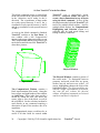
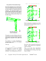
1
TrueGrid
®
“A quality mesh in a
fraction of the time.”
Version 2.1
A Tutorial
Copyright © 2001 by XYZ Scientific Applications, Inc. All rights reserved.
TrueGrid,® the TrueGrid® Manual, and related products of XYZ Scientific Applications, Inc. are copyrighted and distributed
under license agreements. Under copyright laws, they may not be copied in whole or in part without prior written approval
from XYZ Scientific Applications, Inc. The license agreements further restrict use and redistribution.
XYZ Scientific Applications, Inc. makes no warranty regarding its products or their use, and reserves the right to change its
products without notice. This manual is for informational purposes only, and does not represent a commitment by XYZ
Scientific Applications, Inc. XYZ Scientific Applications, Inc. accepts no responsibility or liability for any errors or
inaccuracies in this document or any of its products.
TrueGrid ®is a registered trademark of XYZ Scientific Applications, Inc.
Table of Contents
An Overview . . . . . . . . . . . . . . . . . . . . . . . . . . . . . . . . . . . . . . . . . . . . . . . . . . . . . . . . . . . . . . . . . 1
Introduction to TrueGrid®
The Phases of TrueGrid®
Menus, Dialogue Boxes, and Help . . . . . . . . . . . . . . . . . . . . . . . . . . . . . . . . . . . . . . . . . . . . . . . . 4
The Main Menu
Getting Help For a Main Menu
Sub-Menus
Getting Help For a Submenu Item
Dialogue Boxes
Moving the Cursor in a Dialogue Box
Lists in Dialogue Boxes
Executing a Dialogue Box
Supported Geometry
Importing IGES Files . . . . . . . . . . . . . . . . . . . . . . . . . . . . . . . . . . . . . . . . . . . . . . . . . . . . 10
Internal Geometry Library
Importing IGES Entities
Interactive Graphics
Mouse Selection of Geometry . . . . . . . . . . . . . . . . . . . . . . . . . . . . . . . . . . . . . . . . . . . . . 13
Specifying the Type of Picture
Moving Around Interactively
Drawing a New Picture
Locating Objects Using Labels
Specifying What Objects Get Put in the Picture
Controlling the Picture From the Command Line
A Single Block Part . . . . . . . . . . . . . . . . . . . . . . . . . . . . . . . . . . . . . . . . . . . . . . . . . . . . . . . . . . . 21
Prerequisites
Description
Getting Started
The Geometry
The Block Command
So Now TrueGrid® is in the Part Phase
Configure TrueGrid® to Choose Surfaces by Label
Highlight Faces of the Mesh to be Projected
More About the Part . . . . . . . . . . . . . . . . . . . . . . . . . . . . . . . . . . . . . . . . . . . . . . . . . . . . . . . . . . . 28
How TrueGrid® Built the Mesh
The History Table: Turning Commands Off and On
Interactively Changing the Mesh Density
Clustering of Nodes (Zoning)
Clustering of Nodes (Zoning) in both Directions
Saving and Rerunning the Session File
The Session and Input File Format
Copyright © 2001 by XYZ Scientific Applications, Inc.
TrueGrid® Tutorial
Sphere in a Box:
A Multiple-Block Mesh . . . . . . . . . . . . . . . . . . . . . . . . . . . . . . . . . . . . . . . . . . . . . . . . . . 38
Prerequisites
Description
Creating the Part
What the Block Command is Doing
The Consequences of Having Partitions
Finishing the Mesh
The Peel Commands
About the Mesh
The TrueGrid® Challenge
Mesh Diagnostics
The MEASURE Command
The ELM Command
The Butterfly Mesh:
Rounding a Corner . . . . . . . . . . . . . . . . . . . . . . . . . . . . . . . . . . . . . . . . . . . . . . . . . . . . . . 46
Prerequisites
Description
Creating the Part
The Method
The Geometry
Cutting Corners
Projecting to the Cylinder
The Reason for the Butterfly Mesh
Intersecting Pipes:
A More Challenging Problem . . . . . . . . . . . . . . . . . . . . . . . . . . . . . . . . . . . . . . . . . . . . . 50
Prerequisites
Description
Getting Started
The Geometry
Extracting Curves from Surfaces
Making the Part
Positioning Edges of the Mesh Along Curves and Surface Edges
Interpolation of Intermediate Edges
It’s time to Project
Adding More Nodes
Clustering Nodes near the Pipe Walls
Further Suggestions
Part Replication
Writing the Mesh File
The Double Butterfly Version of the Mesh
Copyright © 2001 by XYZ Scientific Applications, Inc.
TrueGrid® Tutorial
An Overview
Copyright © 2001 by XYZ Scientific Applications, Inc.
TrueGrid® Tutorial
1
Introduction
to
TrueGrid®
TrueGrid® is a general purpose tool for
creating a multiple-block-structured mesh.
Although the beginning of this Tutorial
provides some introductory information, the
new user is strongly advised to read the first 2
chapters of the User’s Manual before
proceeding with this document.
The processes of creating a mesh and creating
geometry are separated within TrueGrid®.
Surfaces and curves may be created internally
or imported from a CAD/CAM system via an
IGES file. A block mesh is then created and
molded to the shape of the geometry.
Making a mesh with TrueGrid® is analogous
to sculpting: A block mesh is created using
the block command. Pieces of the block mesh
are removed so that its topology matches that
of the object to be meshed. Portions of the
mesh are moved, positioned along curves,
projected to surfaces, etc. Interpolation,
smoothing, and zoning requirements are used
to fine-tune the mesh. Parts created separately
are glued (merged) together automatically by
specifying a tolerance.
TrueGrid® is based on a powerful technique
known as the projection method. The
projection method allows faces, edges, and
nodes of the mesh to be directly placed on
surfaces. Similarly, edges and nodes of the
mesh can be placed along curves. In this
sense, TrueGrid® is a constraint-based mesh
generator.
2
Additionally, if TrueGrid® is required to
place two faces of the mesh sharing a common
edge onto two different surfaces, then it will
automatically place the shared edge on the
intersection of the two surfaces. There is no
need to construct the intersection curve of two
surfaces; TrueGrid® will find the intersection
curve automatically. Likewise, a vertex
required to be on three surfaces will be placed
at a common intersection point of all three
surfaces.
Other notable features of TrueGrid® include:
1. TrueGrid® is completely interactive.
2. Any number of commands can be
deactivated and reactivated.
3. TrueGrid® is a WYSIWYG (What you see
is what you get.)-- the actual mesh is shown
at all times.
4. The most frequently used mesh generation
commands can be performed using the
mouse.
5. The mesh can be interactively refined.
6. TrueGrid® produces clean session files
that can be easily edited, rerun, and
interrupted (for interactive mesh editing).
Copyright © 2001 by XYZ Scientific Applications, Inc.
TrueGrid® Tutorial
The Phases of TrueGrid®
TrueGrid® behaves in different ways
depending on what commands have been
issued so far. When the command tg is first
issued, a text and menu window appears on
the screen in the upper left corner. The initial
title of this window is Control Phase. The
title of this particular window will always
indicate the current phase of TrueGrid®.
Because the current phase depends on the
commands issued, the text and menu window
title changes depending on the commands
issued interactively and/or read from a batch
file.
Merge Phase to view boundary conditions, to
diagnose the condition of the mesh, and to
view the highest-quality images of the mesh
and geometry.
As TrueGrid® evolves, the need for the
Control Phase diminishes. Eventually, the
Control Phase will be eliminated in favor of
the Merge Phase. This will make graphics
capabilities available at all times within
TrueGrid®. Most functionality once available
only in the Control Phase has already been
incorporated into the Merge Phase.
The Control Phase, the initial phase of the
code, is where output options are chosen,
material models defined, geometry created,
and where parameters governing the final
mesh output file are set. No graphical
capabilities are available in the Control Phase.
The Part Phase is entered as soon as a block
mesh is created using either the block or
cylinder command. Three new windows
appear in the Part Phase: the Computational
Window (used for displaying logical blocks
of the mesh), the Physical Window (used for
displaying the actual mesh and any geometry),
and the Environment Window (used to
determine what is in a graphics window, how
it is displayed, and how it can be manipulated
using the mouse). It is in the Part Phase
where the mesh is constructed by positioning,
projecting, deleting, zoning, refining and
smoothing parts of the mesh (as well as by
performing other functions).
Boundary
conditions for a part are also specified in the
Part Phase.
The Merge Phase is where parts are
assembled into one model by merging, i.e.,
gluing, nodes together that are within a
specified tolerance of each other. Only the
Computational window of the Part Phase is
missing. Both the Physical and Environment
windows are present in the Merge Phase. It is
in the Merge Phase that the mesh output file is
written. There are features available in the
Copyright © 2001 by XYZ Scientific Applications, Inc.
TrueGrid® Tutorial
3
Menus,
Dialogue Boxes,
and Help
4
Copyright © 2001 by XYZ Scientific Applications, Inc.
TrueGrid® Tutorial
Text/Menu Window, Menus, Dialogue Boxes and Help
The Main Menu
Run TrueGrid® with no input file using the
command
tg
A single window appears in the upper left
corner of the screen. The main menu of
TrueGrid® appears in this text/menu window.
This text/menu window has a title indicating
the current phase of the code (either Control
Phase, Part Phase, or Merge Phase).
Commands can be issued from this window,
and any output such as warnings or error
messages is directed to this window.
press the middle mouse button in the scroll
bar area of the window.
To expand the text area to cover the window
and remove the menu, press the upwardpointing arrow appearing on the right of the
text/menu window, or press the Page Up key
or the Up Arrow key on the keyboard while
the cursor is in the text window. Any of these
actions indicate to TrueGrid® that you wish to
view more of the previous text. In such cases,
the text area expands to fill the window,
thereby making more of the previous text
visible. To scroll through the text, either use
the Page Up, Page Down, Up Arrow or
Down Arrow keyboard keys, or use the scroll
bar. Pressing the left mouse button on the
arrows above the scroll bar moves text by
pages. Pressing the middle mouse button on
the arrows moves the text by lines.
Getting Help For a Main Menu
Because of the limited screen space, the
text/menu window is not particularly large.
This leaves room for other windows that
appear in the other phases of the code.
Consequently, when there is output from
TrueGrid ® to the user, the menu
automatically disappears and the text portion
of the text/menu window is enlarged to fill the
window. For example, enter the illegal
command
In the main menu area of the text/menu
window there are two grey buttons, the
HELP button and the EXIT button.
Press the EXIT button with the left mouse
button to quit TrueGrid ® without
confirmation.
junk
on the command line. A message is issued
indicating that junk is an illegal command.
Notice that the menu is no longer visible.
To bring the menu back, either press the
Enter key or press the right mouse button (3button mouse) in the text/menu window, or
Press the HELP button to activate the help
system. Normally, pressing the left mouse
button on an entry of the main menu causes a
submenu to appear. However, when the
HELP button is on, pressing the left mouse
button on a main menu entry calls up a Help
Window containing information about all the
commands in the given category.
Copyright © 2001 by XYZ Scientific Applications, Inc.
TrueGrid® Tutorial
5
while the HELP button is off.
The Help Window contains a title bar with
scroll arrows as required. Pressing the left
mouse button scrolls by page. Pressing the
middle mouse button scrolls by line. The
Page Up, Page Up, Up Arrow and Down
Arrow keys can also be used for scrolling.
All command names in the category are
highlighted in yellow. A description of the
options for each command and their purposes
is stated.
Each submenu contains two grey buttons: a
MAIN MENU button and a HELP button.
Press the MAIN MENU button to return to the
main menu. The HELP button of a submenu
works the same as that of the main menu.
Each submenu also contains as its first entry a
red button which indicates the name of the
current submenu. The red button is not an
active button.
Getting Help For a Submenu Item
When the mouse is moved onto a command
button in the submenu, a bar appears above
the text/menu window with a short description
of that command.
Pressing the left mouse button on another
category of the main menu replaces the
contents of the current help window with
information about the new category. This
feature allows for easy browsing through all
categories of the menu.
To kill the Help Window, either use window
manager pop-ups or turn the HELP button
off.
Sub-Menus
The help system works the same as for the
main menu, but the Help Window for a
command in a submenu is far more specific.
The first part of the help for a command is in
white with black print. This part is extracted
from the main menu help.
Submenus contain a list of all the commands
in a main-menu category. One uses a
submenu to access detailed help or a
dialogue box for each command in the mainmenu category.
A submenu is viewed by pressing the left
mouse button on a category of the main menu
6
Copyright © 2001 by XYZ Scientific Applications, Inc.
TrueGrid® Tutorial
The second part of the help contains a
complete syntax for the command. All
literal options are in upper-case letters.
Other strings (especially those containing
underscores) are meant to describe the type of
data to be enter. Semicolons should be
regarded as literal.
There are three types of input fields:
1. Fields for entering a single number,
2. Fields for entering a list of numbers,
Dialogue Boxes
Dialogue boxes are available for every
TrueGrid® command. To obtain a dialogue
box for a particular command, move to the
submenu containing that command, and press
the left mouse button on the command
name. (Make sure the HELP button is off.)
®
TrueGrid dialogue boxes can contain
incredibly complex decision trees, especially
for commands used to set options for output to
a particular simulation code.
TrueGrid® dialogue boxes may contain input
fields and option lists as well as descriptions
and/or titles for such.
An input field consists of an optional
description (in white print), prompts (in light
grey print), and cursor boxes (initially green).
There may be many input fields within a
dialogue box. The current active field (the
one to which text input is directed) is always
displayed with a filled green cursor. The
other active cursors are hollow green cursors.
3. Fields for entering general strings.
In the first two cases, input is checked as it is
entered. Characters that would create an
invalid string are ignored. Furthermore, if
just one number is required, then TrueGrid®
will not allow a second number to be entered
into that field.
Moving the Cursor in a Dialogue Box
The active cursor can be repositioned to
another character of the current field, or to
another field entirely using the left mouse
button. Press the left mouse button on the
prompt itself to position the cursor at the end
of the input field. Alternatively, press
RETURN to move the cursor to the next
available field.
If the current field is empty, the cursor can
always be moved from the field. However, if
the current field is non-empty and is not
complete, then TrueGrid® will not allow the
user to move the cursor from the current
field. For example, 1.0e- can be entered, but
is not complete. TrueGrid® informs the user
of such problems by turning the active
cursor blue. The user must correct the
problem before the cursor can be moved to
another field. The user can use the mouse to
move the cursor to a previous character of the
current field. The backspace can be used to
delete a previous character. Or, CTRL+X can
be used to delete the character beneath the
cursor.
Copyright © 2001 by XYZ Scientific Applications, Inc.
TrueGrid® Tutorial
7
When the user presses the ENTER key to end
the current field and begin the next, the
current field is marked "finished" with a red
cursor. The cursor will not return to this field
again without positioning the cursor using the
mouse.
Choose an item of a list by pressing the left
mouse button anywhere on the text of that
entry. The text of the chosen entry will be
highlighted in yellow. To deselect the
entry, press the left mouse button on the
entry again.
Lists in Dialogue Boxes
There are two types of lists that occur in
dialogue boxes: exclusive (choose one) and
non-exclusive (many items can be chosen).
Exclusive lists have entries that begin with a
red ">" character. Non-exclusive lists have
entries that begin with a red "o". An option
title/description is in white above the list.
For example,
When an entry of an exclusive list is chosen,
the other entries disappear from sight. The
hidden entries reappear if the selected entry is
deselected.
Executing a Dialogue Box
Any number of items can be chosen.
Only one item can be chosen.
8
Press the EXECute button at the bottom of
the dialogue box to issue the command. Any
number of error conditions will prevent
execution of the dialogue:
(a) Not all input fields are filled in,
(b) Not all input fields have been flagged
as "complete". Pressing ENTER
causes the field to be checked for
completeness. Complete fields have
red cursors at the end.
(c) No entry has been chosen for a list
that requires a choice to be made.
(d) TrueGrid® is in a state where a
command is in progress.
If (a) or (b) occur, then the input field will be
moved just below the top of the dialogue, and
the prompt for the first offending field is
colored blue. If (c) occurs, then the first entry
of the offending list appears near the top of
the dialogue, and the marker (either ">" or "o"
is colored blue). If (d) occurs, the EXECute
button is colored red.
Copyright © 2001 by XYZ Scientific Applications, Inc.
TrueGrid® Tutorial
To EXECute and QUIT the dialogue box, use
the EXEC/QUIT button. This button is
usually the best choice because it requires the
least number of mouse actions.
Note: Pictures are not automatically redrawn
when commands are issued in TrueGrid®. To
insure that a new picture is drawn, press the
EXEC button or the EXEC/QUIT button
using the middle mouse button instead of the
left mouse button. Doing so causes a draw
command to be issued with the command.
Copyright © 2001 by XYZ Scientific Applications, Inc.
TrueGrid® Tutorial
9
Supported Geometry
Importing IGES Files
10
Copyright © 2001 by XYZ Scientific Applications, Inc.
TrueGrid® Tutorial
Internal Geometry Library
TrueGrid® can create a wide variety of
surface types such as:
sphere
plane
cylinder
cone
torus
surface of revolution
ruled surface
swept surface (using skinning)
extruded surface (general cylinders)
surface interpolated between two
other surfaces
tabulated surface consisting of
a 2D array of points
surface composed of multi-sided
polygons
pipe surface from a 3D curve
surface given by equations
cubic spline surface
B-spline surface
NURBS surface
Stereo Lithography surfaces
compositions of any of the above
An extensive set of options for building 2D
and 3D curves is also provided within
TrueGrid®.
For more information, issue the help
command for ld in the 2D CURVE sub-menu,
sd is the SURFACE sub-menu, or curd in the
3D CURVE sub-menu.
Importing IGES Entities
TrueGrid® can extract most surface and curve
entities from an IGES file. We presently
support the following IGES Entities:
100 - Circular Arc
102 - Composite Curve
104 - Conic Arc
108 - Plane
110 - Line
112 - Parametric Spline Curve
114 - Parametric Spline Surface
118 - Ruled Surface
120 - Surface of Revolution
122 - Tabulated Cylinder
124 - Transformation Matrix
126 - NURBS Curve
128 - NURBS Surface
140 - Offset Surface
142 - Curve on a Parametric Spline Surface
144 - Trimmed Parametric Spline Surface
402 - Associativity Instance
Extracting All IGES Entities
All supported entities are extracted from an
IGES file with the single command
Issuing this command causes the specified
IGES input file to be read and all curves and
surfaces to be extracted. You can find this
command in the CAD sub-menu. The
surfaces are assigned TrueGrid® surface
definition numbers beginning with m, and the
curves are assigned TrueGrid® curve
definition numbers beginning with n (where m
and n are integers.) Note that curves used to
construct others are not processed.
Selectively Extracting IGES Entities
Entities can be selectively extracted from an
IGES file using a two-step process. First,
specify the IGES file using the command (also
in the CAD sub-menu)
igesfile IGES_file_name
Second, use either the igescd, igessd,
or nurbsd command to extract curves,
surfaces, or NURBS surfaces, respectively.
These commands are all found in the CAD
sub-menu, as well.
iges IGES_file_name m n;
Copyright © 2001 by XYZ Scientific Applications, Inc.
TrueGrid® Tutorial
11
Example:
igesfile
nurbsd 1
igessd 1
igescd 1
airplane.igs
24 1;
15 25;
87 2;
will cause TrueGrid® to
(a) read the IGES file ’airplane.igs’;
(b) to extract the first 24 NURBS surfaces,
and to create TrueGrid® surface definitions 1
to 24;
(c) to extract the first 15 surfaces (other than
NURBS), and to create TrueGrid® surface
definition numbers 25 to 40;
(d) to extract the first 87 curves from the
IGES file, and to create TrueGrid® curve
definition numbers 2 to 88.
The useiges command is also
found in the CAD sub-menu.
TrueGrid® will process this set of commands
many times faster than it was able to process
the commands in the previous example.
Notes about saveiges
1. Only entities processed before the
saveiges command are saved. (Entities are
processed when either igessd, igescd,
or nurbsd are issued.)
2. The name of the file used with the
saveiges and the useiges commands
must match exactly, or the binary IGES file
will not be used.
3. The name of the file used with either the
igesfile or iges command must be
exactly the same as when saveiges was
issued.
Saving Time
Large IGES files may take some time to
process within TrueGrid®. It can be timeconsuming to tile all the surfaces for graphics
purposes. Every time TrueGrid® is rerun and,
consequently, asked to read the same IGES
file, all this work must be repeated. To
eliminate the need for subsequent processings
of an IGES file, use the command
IGES Levels (Layers) and Groups
The layer or level feature commonly found in
CAD systems can be used to organize the
geometry for TrueGrid® use.
The
associativity instance is used for grouping the
entities into levels. TrueGrid® preserves this
level structure.
saveiges binary_output_file
Example: Suppose that after issuing the
previous set of commands, the command
saveiges airplane.bin
is issued. Then the next time the same set of
surfaces and curves are to be used, issue the
commands
useiges airplane.bin
igesfile airplane.igs
nurbsd 1 24 1;
igessd 1 15 25;
igescd 1 87 2;
12
Copyright © 2001 by XYZ Scientific Applications, Inc.
TrueGrid® Tutorial
Interactive Graphics
Mouse Selection of Geometry
Copyright © 2001 by XYZ Scientific Applications, Inc.
TrueGrid® Tutorial
13
TrueGrid® Graphics
TrueGrid® provides dynamic control for
rotating, translating, and zooming. Also
provided is readily accessible control over
what curves, surfaces, regions, etc. are in the
picture and whether or not they are labeled.
Example:
Run TrueGrid® using the
command tg with no command-line options.
There is no graphics capability in the Control
Phase of the code, so issue the command
merge
to enter the Merge Phase of the code.
Next create a couple of surfaces using the
Surface Definition command:
sd 1 cyli
sd 2 plan
0 0 0
-1 0 0
0 1 0
1 0 0
2
The first surface is a right circular cylinder of
radius 2 whose axis of rotation passes through
(0,0,0) and is parallel to (0,1,0). The second
surface is a plane passing through (-1,0,0) and
normal to (1,0,0).
The default angle of perspective is 23 degrees.
Setting the angle to 0 eliminates all effects of
perspective.
Specifying the Type of Picture
The current picture in the Physical Window
should appear similar to the one below
Even though the plane is actually
perpendicular to the x-y plane, it appears
somewhat slanted.
This is because
perspective is added to the picture, i.e.,
distant parts of the picture are smaller. The
various circular cross sections of the cylinder
differ from each other for the same reason.
The perspective angle (the angle between the
center of the picture and the edge of the
screen) is controlled by the command
angle angle_of_perspective .
14
TrueGrid® can create several types of
pictures. Which type of picture will be
generated depends on the setting of the
Picture button group in the Environment
Window of TrueGrid® (shown above). The
initial setting of the picture type is a Hide
drawing (hidden lines are removed). The
other types are described below. To choose a
different picture type for all subsequently
generated pictures, press the left mouse
button on the desired picture type button
(Wire, Hide or Fill). Changing the picture
type does not cause a picture to be
regenerated. A picture is redrawn by pressing
either the Draw, Center or Restore button.
Copyright © 2001 by XYZ Scientific Applications, Inc.
TrueGrid® Tutorial
The simplest type of picture is a Wire frame
drawing of all objects in the picture (the
preceding picture is an example). Objects that
would be hidden by others (in the real world)
are not hidden in a Wire picture.
surfaces are removed. For all but the PC
Version, a two-source lighting model is
used (along with dithering to create a very
smoothly lighted picture when only 8 bit plane
graphics is available.)
Picture Type: Wire
Picture Type: Fill
The Hide option is used for creating pictures
whose hidden lines are removed.
When the picture type is set to Fill, several
options concerning the lighting model can be
changed via a pop-up menu which is accessed
with the right mouse button in the Physical
Window (not applicable to the PC version).
Picture Type: Hide
Hardware Graphics. We currently support
hardware graphics features only for SGI
versions of TrueGrid®. To invoke the
graphics hardware features (lighting, fogging,
material models, etc.), press the H.W. button
using the left mouse. When hardware is
invoked, the Wire option is the same as
before, except that lighting and fogging
models now apply. The Hide and Fill options
no longer function differently; both set the
picture type to a Fill type. Many parameters
of the hardware model can be interactively
changed using the right mouse button to
activate a pop-up menu in the Physical
Window.
The Fill option is used to create a picture
where all polygons are filled and all hidden
Copyright © 2001 by XYZ Scientific Applications, Inc.
TrueGrid® Tutorial
15
Moving Around Interactively
The Middle Mouse Button is used to
manipulate 3D graphics windows in
TrueGrid®. The effect of pressing the middle
mouse button in either the Physical or
Computational window depends on which of
the four buttons, Rotate, Move, Zoom or
Frame is pressed. The buttons in this Motion
button group of the Environment Window
(pictured above) are reset by pressing the
desired button using the left mouse button.
The Rotate, Move and Zoom options are all
similar in nature. A dynamic operation is
performed on the picture by moving the
mouse to either the Physical or Computational
Window, pressing the middle mouse button,
and dragging the mouse to a new position
while the middle mouse button remains
pressed. As the mouse is moved, a minimal
wire-frame representation of the picture is
redrawn as quickly as possible. When the left
mouse button is finally released, a new picture
is redrawn. The type of the final picture is
determined by the setting of the Wire, Hide,
Fill button group.
Rotate. Horizontal movement of the mouse
causes a rotation about a vertical line parallel
to the screen plane. Vertical movement of the
mouse causes a rotation about a horizontal
line parallel to the screen plane. When the
picture is magnified, rotations are reduced
appropriately. This effect is eliminated by
holding the “Shift” key down while rotating.
Move. The picture follows the mouse.
Zoom. Only vertical mouse movement causes
a change. Move the mouse upward to enlarge
the picture, and downward to shrink the
picture. Moving the mouse half a window
causes the picture to change by a factor of 10.
Frame. The Frame option is the fastest way
to isolate some visible portion of the current
16
picture. This is done by positioning a rubberbanded box around the part of the picture to
be isolated; the framed part of the picture is
then expanded to fill the entire graphics
window. To frame part of the picture, first
make sure the Frame button is pressed. Move
the mouse into the graphics window and press
the middle mouse button where you wish to
place one corner of the framing box. Keep the
middle mouse button pressed and drag the
mouse to a new position. A rubber-banded
square box will appear. Release the middle
mouse button to view a wire frame, a hiddenline, or a polygon fill picture of the contents of
the framing box (depending on the setting of
the Wire, Hide, Fill buttons). To abort a
frame operation in progress, drag the mouse
outside of the graphics window and release
the middle mouse button.
Drawing a New Picture
It is sometimes necessary to tell TrueGrid® to
redraw the picture. This is especially true in
the Part Phase, where commands are buffered
– all buffered commands are executed
whenever a new picture is generated. Also, if
the user changes the type of picture to be
drawn (Wire, Hide, Fill option), a new picture
is not automatically redrawn; the user needs to
tell TrueGrid® to redraw the picture.
There are three basic ways to regenerate the
picture. The first uses the Draw option.
Invoking the Draw option (by pressing the
Draw button with the left mouse button)
causes the code to execute all buffered
commands, and to generate a picture of the
specified type (Wire, Hide or Fill) in the same
position and orientation as the previous
picture.
The Center option is used to adjust the picture
so that all objects are fully visible within the
window. The Center command leaves the
rotational orientation of the picture the same
as for the previous picture.
Copyright © 2001 by XYZ Scientific Applications, Inc.
TrueGrid® Tutorial
The Restore option also makes sure all objects
are visible. However, the Restore command
puts the picture back to the home (default)
rotational orientation.
The Center and Rest commands are especially
useful when objects are added or removed
from the picture, or if the user gets lost in the
picture.
Locating Objects Using Labels
Labels play an important role in interactive
mesh generation. TrueGrid® allows the user
to reference an object by pointing to its label.
TrueGrid® never draws overlapping labels
and, within this restriction, tries to center the
label on the object. Furthermore, TrueGrid®
highlights the object corresponding to a
particular label when the user points to that
label. (Assuming that the user has selected
the “Labels” option under the “Pick” menu.)
These features make it easy to find a particular
object by its label, even when there are many
objects in the picture.
Only one class of objects is labeled at any
given time. The user selects the class of
objects to be labeled by first selecting the
Labels Dialogue of the Environment
Window by pressing the Labels button with
the left mouse button. Then the user presses
the button corresponding to the class of
objects to be labeled. Pressing the Off button
removes all labels.
mouse button anywhere else in the picture
clears the highlighting.
Next press the Surf Point button. Points on
the plane (used mainly for graphical purposes)
are now labeled. TrueGrid® allows the user
to attach points of the mesh directly to such
surface points. Zooming in on part of the
picture will reveal more labels and points that
can be used while building the mesh.
The Surf Edge button will label the edges of
all defined surfaces in the picture. Edges of
the mesh can be directly placed on such
surface edges. When surfaces are infinite, as
in the example, they have no useable edges;
their edges can be displayed and highlighted
but cannot be used in interactive meshing.
This is because edges of infinite surfaces
change, depending on the size of the bounding
box for the picture.
Example. (Continuing with the current
example.) Press the Surface button to display
labels for the plane and cylinder in the picture.
Move the mouse into the Physical Window
and press the left mouse button on one of the
two labels in the picture. Pointing in this
fashion to label 1 highlights surface definition
1, which is the cylinder. Similarly, pointing to
label 2 highlights the sphere. Pressing the left
Copyright © 2001 by XYZ Scientific Applications, Inc.
TrueGrid® Tutorial
17
Specifying What Objects Get Put in the Picture
The Display List dialogue of the
Environment Window provides an
interactive way to add and remove objects
from the picture. Pressing the Display List
button of the Environment Window activates
this dialogue.
The group of buttons on the left is used to
select the class of objects to which commands
in this dialogue will apply. The group of
buttons on the right execute commands to
selectively add objects to or remove objects
from the picture.
Removing an Object from the picture is done
by highlighting the object (using the label
highlighting feature described above), and
then by pressing the Remove button with the
left mouse button.
To Remove All Objects Except One,
highlight the object to remain (using the label
highlighting feature described above),
18
and then press the Show Only button with the
left mouse button.
Remove All Objects of the Specified Class
by pressing the Show None button with the
left mouse button. Removing all surfaces, for
example, makes the mesh easier to view.
Add All Objects of the Specified Class to
the picture by pressing the Show All button
with the left mouse button.
The Add Feature also works on selected
objects.
Using the Computational
Highlighting System for the mesh in the Part
Phase, it is possible to select a region of the
mesh that is not in the picture. Such a region
is then added to the picture by pressing the
Add button with the left mouse button.
Notice that the Region button is grayed out in
the Merge Phase because it is not possible to
point to a region of the mesh in this phase of
the code.
Copyright © 2001 by XYZ Scientific Applications, Inc.
TrueGrid® Tutorial
Controlling the Picture From the Command Line
All of the interactive functions presented so
far (except for the frame feature) correspond
to commands that can be issued from the text
and menu window of TrueGrid®. On the
other hand, there are graphics commands that
have no interactive counterparts. For
Generate a New Picture
Generate a line drawing
draw
Generate a hidden-line drawing
disp
Generate a polygon fill drawing
tvv
Center the picture (do not change the
rotational orientation)
center
Center the picture in the default orientation
(with no rotations)
rest or restore
Rotate, Translate, Zoom
Rotate the picture about a horizontal line
parallel to the screen plane
rx angle_in_degrees
Rotate the picture about a vertical line parallel
to the screen plane
ry angle_in_degrees
Rotate the picture about a line perpendicular
to the screen plane
rz angle_in_degrees
Zoom Forward by a factor (that can be less
than 1)
zf zoom_factor
Zoom Backward by a factor (that can be
greater than 1)
zb inverse_zoom_factor
Label Objects in the Picture
example, there is no interactive command to
add a surface, curve, etc. to the picture.
Presented below is a list of TrueGrid®
commands that are analogous to the
interactive functions presented so far.
sdpt - to label points on surfaces
crvpt - to label points on curves
off - to remove all labels
Specify the Surfaces Shown
Display All Surface Definitions
dasd
Remove All Surface Definitions
rasd
Display a single Surface Definition
dsd surface_definition_number
Display a list of Surface DefinitionS
dsds list_of_surface_definitions ;
Add a Surface Definition
asd surface_definition_number
Remove a Surface Definition
rsd surface_definition_number
Specify the Curves Shown
Display All Curve Definitions
dacd
Remove All Curve Definitions
racd
Display a single Curve Definition
dcd curve_definition_number
Display a list of Curve DefinitionS
dcds list_of_curve_definition_numbers ;
Add a Curve Definition
acd curve_definition_number
Remove a Curve Definition
rcd curve_definition_number
labels option
where option can be
sd - to label surfaces
crv - to label curves
sdedge - to label surface edges
Copyright © 2001 by XYZ Scientific Applications, Inc.
TrueGrid® Tutorial
19
Specify the Parts Shown
Display All Parts
dap
Display one particular Part
p part_number
Add a Part to the picture
ap part_number
Remove a Part from the picture
rp part_number
Specify the Materials Shown
Display All Materials
dam
Display a specific Material
m material_number
Add a Material to the picture
am material_number
Remove a Material from the picture
rm material_number
20
Specify the Regions Shown
These commands apply only in the Part Phase.
The distinction between a Region
specification and an Index Progression
specification are explained later.
Display All Regions
darg
Display a specific Region
rg region
Display a Region specified by Index
Progression
rgi progression
Add a Region to the picture
arg region
Add a Region specified by Index Progression
argi progression
Remove a Region from the picture
rrg region
Remove a Region specified by Index
Progression
rrgi region
Copyright © 2001 by XYZ Scientific Applications, Inc.
TrueGrid® Tutorial
A Single Block Part
Copyright © 2001 by XYZ Scientific Applications, Inc.
TrueGrid® Tutorial
21
Making a Single Block Part
Introduced Here:
The Block Command
Projection Method
Intersection Algorithm
Computational
Highlighting System
Interpolation
Prerequisites
The previous sections on interactive graphics,
labeling objects, and choosing objects by
label.
Description
A single block part is created. Each of the six
faces in projected to a different surface to
form a rounded-end rod.
TrueGrid® automatically places the edges of
the block along intersections of the surfaces.
The corners of the block are automatically
placed at the intersections of three surfaces.
The default interpolation takes care of the
interior nodes.
Getting Started
The Geometry
Run TrueGrid® with no input file. Enter the
Merge Phase by typing the command
The mesh is determined by just a few
surfaces. The commands to create the
geometry are listed below.
merge
followed by a return. This allows you to view
the geometry for this problem as it is being
created.
sd
sd
sd
sd
sd
1
2
3
4
5
cyli 0 0 0 0 1 0 2
plan -1.5 0 0 1 0 0
plan 1.5 0 0 1 0 0
sphe 0 -3 0 2.5
sphe 0 3 0 2.5
As an experiment, enter only part of a given
command before pressing ENTER.
TrueGrid® will prompt you for the next
required parameter of the command. You
may enter as much of the command after the
prompt as you wish (even part of the next
command).
22
Copyright © 2001 by XYZ Scientific Applications, Inc.
TrueGrid® Tutorial
Pressing the ESCape KEY in the middle of a
command aborts that command. Another way
to correct any mistake is to simply redefine
the surface.
Surface Definition 1 is a right circular
cylinder of radius 2 whose axis of rotation
passes through (0,0,0) and is parallel to
(0,1,0). Both the front and back faces of the
rod will lie on this cylinder
Surface Definition 2 is a plane passing
through the point (-1.5,0,0) and perpendicular
to (1,0,0). The left face of the rod will lie on
this plane.
Surface Definition 4 is a sphere centered at
(0,-3,0) and of radius 2.5. The bottom end of
the rod will lie on this sphere.
Surface Definition 5 is a sphere centered at
(0,3,0) and of radius 2.5. The top end of the
rod will lie on this sphere.
The Block Command
The actual mesh is now created using the
block command. At the merge> prompt
enter
block
Surface Definition 3 is a plane passing
through the point (1.5,0,0) and perpendicular
to (1,0,0). The right side of the rod will lie on
this plane.
1 9; 1 10; 1 8;
-2 2;-6 6;-2 2;
(The command can be entered on one line or
split across lines as shown.)
Copyright © 2001 by XYZ Scientific Applications, Inc.
TrueGrid® Tutorial
23
So Now TrueGrid® is in the Part Phase
This block command creates a single block
mesh with 9 nodes in the i-direction, 10 nodes
in the j-direction, and 8 nodes in the kdirection. The x-coordinates of these nodes
are evenly spaced between -2 and 2, the ycoordinates evenly spaced between -6 and 6,
and the z-coordinates evenly spaced between
-2 and 2.
As soon as the block command is finished,
TrueGrid® switches to the Part Phase. A
new window with a title Computational
appears in the upper right corner of the screen.
The Computational and Physical pictures will
not be drawn until the user tells TrueGrid® to
draw these pictures.
TrueGrid® was a single-block mesh.
However, TrueGrid® allows the user to
create a three-dimensional array of blocks
using the block command. In fact, all but
the simplest meshes built with TrueGrid® will
tend to be multiple-block meshes. And for
multiple-block meshes, the Computational
Highlighting and Selection system is a
powerful tool for both mesh editing and
setting boundary conditions.
Physical Window
Computational Window
The Computational Window contains a
block representation of the mesh. Along the
lower, upper, and right borders of the window
are index bars. These index bars provide a
means by which the user can select any
corner, edge or face of the block, as well as
the solid block. Such a selection can then be
used directly in any command requiring a
description of part of the mesh as one of its
arguments.
The Physical Window contains a picture of
the actual mesh. To distinguish between
geometry and mesh, mesh lines are green,
surfaces are red, and curves are yellow. Of
course, highlighting changes the color of the
highlighted object. The green mesh lines are
not just a rough representation of the mesh.
Any time the user redraws the physical
window, all buffered commands are executed
and the actual mesh is displayed.
The computational picture would not be so
useful if all that could be created within
24
Copyright © 2001 by XYZ Scientific Applications, Inc.
TrueGrid® Tutorial
Setting the Window
Because there are two graphics windows in
the Part Phase, it is necessary to inform
TrueGrid® which window is to be acted upon.
This is done by pressing the left mouse
button on either the Physical, Computational
or Both button.
When either the Draw, Center or Restore
buttons is pressed, the appropriate window is
redrawn. The same is true of manually issued
commands such as rx, ry, rz, etc. The user
should also be aware that commands such as
those to reset the angle of perspective are also
directed to the window indicated by the
setting of Phys, Both and Comp button
group.
Configure TrueGrid® to Choose Surfaces by Label
There are three different functions for the
left mouse in the Part Phase Physical
Window. The left mouse button can be used
to choose objects by their labels, to choose
the nearest mesh vertex, and to interactively
move portions of the mesh. You must
explicitly tell TrueGrid® which of these
actions to perform. (There was no need to do
this in the Merge Phase, because the left
mouse button was used only to highlight a
labeled object.)
Finishing the problem at hand requires a few
interactive projections.
An interactive
projection requires the user to highlight a face
of the mesh, and to highlight a surface.
Therefore, for the purposes of projection,
press the Pick button in the Environment
Window to obtain the Pick Dialogue pictured
above. Then press the Label button to inform
TrueGrid® that you wish the left mouse
button to be used to pick an object by its label.
Notice the sketch of the mouse with the left
mouse button marked. All functions using the
left mouse button in the Physical Window are
clearly marked in this manner.
Now TrueGrid® is set up to pick a surface by
its label. So highlight the cylinder by finding
the appropriate label (this is surface definition
1).
Highlight Faces of the Mesh to be Projected
The front and back faces of the mesh are to be
projected to the cylinder that was just
highlighted.
These faces can be
simultaneously selected for just this purpose.
The Computational Highlighting System of
TrueGrid® is the general purpose tool for
selecting and examining parts of the mesh.
The first component of this unique
highlighting system is a Slicing Plane
(illustrated below). The slicing plane feature
is activated whenever the mouse is moved into
the Computational Window near one of the
dots of the index bars. The dot near the
mouse turns white, and a corresponding block
Copyright © 2001 by XYZ Scientific Applications, Inc.
TrueGrid® Tutorial
25
face in the Computational Window is
highlighted in white.
convention, the actual values of fixed indices
increase from left to right and bottom to top.
Now select the back face of the mesh by first
highlighting that face (as shown above) and
then by pressing the left mouse button while
the minimum constant k slicing plane is
active. The back face of the computational
block and the back face of the mesh will both
turn yellow.
If you make a mistake while making the
selection, press the F2 KEY to clear the
selection (this will not clear any slicing plane).
The Minimum k Slicing Plane
The corresponding mesh face in the Physical
Window is also highlighted in white.
Next move the mouse until the maximum k
slicing plane is active (equivalently, when the
right dot on the top index bar is white). The
highlighted face of the mesh is the front face.
Add this face to the current selection by
pressing the left mouse button while the
maximum k slicing plane is still active.
At this point, both the front and back faces of
the mesh will be highlighted in yellow. The
two dots of the upper index bar will be red.
The cylindrical surface you highlighted earlier
should still be highlighted.
The final
computational selection appears below.
Corresponding Physical Mesh Face
Notice that, in this example, when the mouse
is near the left-most dot of the upper index
bar, that the back face of mesh is highlighted.
Dots on the lower index bar correspond to
faces where the i-index is held constant; dots
on the right index bar correspond to constant
j-index faces; dots on the top index bar
correspond to constant k-index faces. By
26
Front and Back Faces Selected
Copyright © 2001 by XYZ Scientific Applications, Inc.
TrueGrid® Tutorial
It should not be difficult to finish this
problem. There are four other projection
commands required. The minimum i-face
should be projected to the plane on the left
(surface definition 2). The maximum i-face
should be projected to the plane on the right
(surface definition 3). The minimum j-face
(bottom) should be projected to the bottom
sphere (surface definition 4). The maximum
j-face (top) should be projected to the top
sphere (surface definition 5). Keep in mind
that the F2 KEY clears the computational
selection, and that Undo will reverse the
effects of any meshing command such as a
projection.
Front and Back Mesh Faces
Now that the faces of the mesh to be projected
and the surface to which they are to be
projected are both highlighted, then the
required projection can be performed.
In the next sections, there is more about the
activating and deactivating commands, more
about the computational highlighting system,
and information concerning how this single
block mesh is handled internally. All of these
sections reference this example.
Perform the projection of the highlighted
mesh faces to the highlighted surface by
pressing the Project button.
In case of a mistake, deactivate the projection
command by pressing the Undo button in the
Edit button group of the Environment
Window.
Pressing the Undo button will undo the last
active meshing command. So pressing the
Undo button many times will undo many
meshing commands. (The Undo feature does
not apply to graphics commands.) There are
more sophisticated ways to selectively
deactivate meshing commands.
Such
techniques will be discussed later.
Copyright © 2001 by XYZ Scientific Applications, Inc.
TrueGrid® Tutorial
27
More About the Part
28
Copyright © 2001 by XYZ Scientific Applications, Inc.
TrueGrid® Tutorial
How TrueGrid® Built the Mesh
The previous example provides a wonderful
illustration of the projection method of
TrueGrid®. For this previous example, we
describe the method used by TrueGrid® to
build the single block mesh. Snapshots of the
mesh in various unfinished states are used for
illustration purposes. You never actually see
the intermediate pictures.
Step 1: TrueGrid® begins with the corners of
the block (or blocks, for a multiple-block
mesh). In the case at hand, each corner of the
mesh is required to be on 3 different surfaces.
So TrueGrid® first places each corner at the
intersection of the 3 surfaces on which the
corner is to lie.
Step 2: Interpolate Edges
Step 3: The edges of the blocks are now
projected to the surfaces on which they must
lie. In this example, all edges are required to
be on two different surfaces. So TrueGrid®
places all the interior nodes of a given edge
onto the intersection of the two surfaces on
which these interior edge nodes are to lie.
Then TrueGrid® equally spaces these nodes
along this intersection curve (because there
are no clustering requirements in this case).
Step 1: The Corners are Positioned
Step 2: After the corners of a block are
positioned, the edges are interpolated using
the default interpolation method of
TrueGrid®. For edges this amounts to pulling
the edges tight as though they were strings,
and then evenly spacing the nodes along the
edges.
Step 3: Edges are Projected
Copyright © 2001 by XYZ Scientific Applications, Inc.
TrueGrid® Tutorial
29
Step 4: Using the edges, all faces of the mesh
are now interpolated. Many faces end up (by
accident) in their final positions.
For
example, the faces that must lie on planes
have edges that already lie on planes and,
consequently, the interpolated faces end up on
planes. However, the top and bottom ends of
the rod are not correctly positioned. The top
and bottom ends are required to be on spheres.
Step 5: Block Faces are Projected
Step 6: As a final step, the interior nodes of
the block are interpolated using the positions
of the nodes on the block faces. The mesh is
complete.
Step 4: Interpolate Block Faces
Step 5: The interior nodes of faces of the
mesh are now projected onto the surfaces on
which they are required to lie. Nearly all
nodes were already correctly positioned (by
accident). Only the top and bottom ends of
the rod, which must lie on spheres, end up
being repositioned.
At this point the mesh appears to be finished.
However, there is no telling where the interior
nodes may be at this point. Because the
interior nodes of the block (not pictured) have
never been touched, it is even possible that
some of these nodes now lie outside the
volume of the actual problem.
Step 6: Interpolate Interior Block
Nodes
There is no difference between the last
picture and the previous because interior
nodes are not shown in either.
30
Copyright © 2001 by XYZ Scientific Applications, Inc.
TrueGrid® Tutorial
The History Table: Turning Commands Off and On
A History Table of commands is kept by
TrueGrid®. All the commands in the history
table can be viewed by pressing the History
button in the Edit button group of the
Environment Window.
command: active, deactivated, or inactive.
Immediately following the status is a
command sequence number. Command
sequence numbers are assigned sequentially
when the command is issued. The last part of
the first line contains a brief description of
the command. The next line begins either
with region or progression, indicating which
of the two ways of specifying part of the mesh
was used.
The history is also summoned by entering the
history
command at the text window prompt.
The history appears in the text/menu
window. The entire history table will
probably not be visible at one time. There are
several solutions to this problem. Put the
mouse in the text/menu window and using the
up arrow, down arrow, page up or page
down keys to scroll the text. Alternatively,
use the scroll bar on the right side of the
window. Another solution is to enlarge the
window.
For the present example, the history table
contains all the projection commands. (The
order of the commands in the table depends on
the order in which they were issued.)
H I S T O R Y
T A B L E
active 2 surface projection
progression 1 2; 1 2; -1 0 -2;
active 3 surface projection
progression -1 1; 1 2; 1 2;
active 4 surface projection
progression -2 2; 1 2; 1 2;
active 5 surface projection
progression 1 2; -2 2; 1 2;
active 6 surface projection
progression 1 2; -1 1; 1 2;
Each entry of the history is composed of two
lines. The first line of each entry begins with
one of three words indicating the status of the
Highlighting the Part of the Mesh
to which a Command Applies
Press the middle mouse button anywhere on
the second line of the history entry for a
command to highlight the part of the mesh to
which a command applies. (This line begins
with either "progression" or "region".) Notice
that both the computational and physical
windows are highlighted. This highlighted
region can be used in subsequent commands,
or modified and used in subsequent
commands.
Deactivating and Reactivating
Commands
To deactivate a command whose status is
"active", press the middle mouse button on
the word "active". A command is generated
on the command line which, when issued, will
deactivate the given command. Press return to
issue this command. Multiple commands can
be issued at one time. Redraw the picture to
see the result.
To reactivate a command whose status is
"deactivated", press the middle mouse button
on the word "deactivated". A command is
generated on the command which, when
issued, will reactivate the given command.
Press return to issue this command. Multiple
commands can be issued at one time. Redraw
the picture to see the result.
Example. Use the history highlighting
feature to isolate the command requiring the
Copyright © 2001 by XYZ Scientific Applications, Inc.
TrueGrid® Tutorial
31
top end of the rod to be projected. The
progression line of that command appears as
progression 1 2; -2 2; 1 2;
active 6 surface projection
progression 1 2; -1 1; 1 2;
progression 1 2;-2 2;1 2;
On the line just above the progression
description, press the middle mouse button on
the word "active". A command such as
decmd 5
appears on the command line of the text/menu
window.
Press ENTER to issue this
command. A picture is not automatically
regenerated, so press the Draw button in the
environment window.
Notice that the history table reports the status
of the command you selected to be
"deactivated".
Reactivate the command by pressing the
middle mouse button on the word
"deactivated", and by pressing ENTER.
Again, draw the picture to see that the top end
of the rod is back on the sphere. Pressing the
History button will print a history table that
reports the command status to be active.
Inactive commands cannot be deactivated.
Such commands only occur when using
certain very advanced features of TrueGrid®.
No such examples occur in this tutorial.
The Top End is not Projected
to the Sphere Anymore
Notice that the top end of the bar is no longer
projected to the sphere. Press the History
button again to see the new history table.
H I S T O R Y
T A B L E
active 2 surface projection
progression 1 2; 1 2; -1 0 -2;
active 3 surface projection
progression -1 1; 1 2; 1 2;
active 4 surface projection
progression -2 2; 1 2; 1 2;
deactivated
5
surface
projection
32
Copyright © 2001 by XYZ Scientific Applications, Inc.
TrueGrid® Tutorial
Interactively Changing the Mesh Density
Modify SEQuence (mseq)
The mseq command is used to change the
mesh density. For example, the block
command
block 1 9; 1 10; 1 8;
-2 2;-6 6;-2 2;
creates the same mesh as these commands
block 1 2; 1 2; 1 2;
-2 2;-6 6;-2 2;
mseq i 7
mseq j 8
mseq k 6
The first mseq command adds 7 nodes in the
i-direction. The next mseq command adds 8
nodes in the j-direction. The last mseq
command adds 6 nodes in the k-direction.
The Original Mesh
The mseq command can also be used to
remove nodes in one direction by using a
negative number.
Refining the Mesh of the Previous
Example. Just to illustrate how easy it is to
refine the mesh without having to change any
other commands, try the command
mseq j 10
To view the change, regenerate the picture by
pressing the draw button.
The effects of this command are reversed by
the command
After the MSEQ Command
mseq j -10
As before, press the Draw button to view the
changes to the mesh.
Copyright © 2001 by XYZ Scientific Applications, Inc.
TrueGrid® Tutorial
33
Clustering of Nodes (Zoning)
Relative Spacing Command (res)
SYNTAX:
res i_min j_min k_min i_max j_max k_max direction ratio
where
direction can be either i, j, or k, and
ratio is a positive floating point number.
DESCRIPTION:
The nodes of all block edges of a specified region of the mesh
are clustered in the specified direction. The amount of clustering
depends on the ratio. The nodes are spaced so that the ratio of
distances between adjacent nodes in the specified direction equals
the given ratio.
Thus, for example, if re-spacing is specified in the i direction
with a ratio of 1.2, then the nodes with smaller i-index values are
closer together than those with larger i-index value. In particular,
for a fixed j and k index, the distance between the nodes with i-index
2 and 3 will be 1.2 times as large as the distance between nodes with
i-index 1 and 2. So in this case, nodes "cluster" in the negative
i-direction.
Example. To cluster the nodes of the bar
toward the bottom end of the bar, issue the
command
res
1 1 1 2 2 2
j
1.1
To avoid typing the region description, first
clear the computational highlighting by
pressing the F2 KEY. Then type res on the
command line, and press the F1 KEY. A
description of the highlighted region is put
onto the command-line following res.
Because a null selection makes no sense in a
command, TrueGrid® converts the null
selection to a description of the entire mesh.
Finish the command by entering j 1.1.
34
Zoning in the j-direction
Copyright © 2001 by XYZ Scientific Applications, Inc.
TrueGrid® Tutorial
Clustering of Nodes (Zoning) in both Directions
Double Relative Spacing Command (drs)
SYNTAX:
res i_min j_min k_min i_max j_max k_max direction ratio1 ratio2
where
direction can be either i, j, or k
ratio1 is a positive floating point number
ratio2 is a positive floating point number
DESCRIPTION:
The nodes of the specified region are clustered in a
given direction. Zoning near the minimum index of the given
direction is controlled by the first ratio. Zoning near the
maximum index of the given direction is controlled by the
second ratio. If the second ratio is the reciprocal of the
first, then drs works the same way as res.
Example. The drs command is particularly
useful for fluids problems where nodes need
to be clustered toward the walls of a mesh in
order to resolve the boundary layer. To
achieve such clustering for the current
example, issue the three commands
drs 1 1 1 2 2 2
drs 1 1 1 2 2 2
drs 1 1 1 2 2 2
i
j
k
1.2 1.2
1.2 1.2
1.2 1.2
To avoid typing the region each time, use the
same procedure described in the example of
the res command.
NOTE: If you have already issued the res
command of the previous example, there is no
need to deactivate that command. Zoning
commands for a region override previously
issued zoning commands for that region.
Double Zoning in all 3 Directions
Copyright © 2001 by XYZ Scientific Applications, Inc.
TrueGrid® Tutorial
35
Saving and Rerunning the Session File
A TrueGrid® session file is written every time
that TrueGrid® is run. If no session file name
is specified on the command line (using the
s= option), then the session file is named
tsave and is placed in the current working
directory. If the session file is named tsave,
then make sure to rename the session file
when finished, or it will be over-written the
next time TrueGrid® is run.
Rerunning the Session File
A session file can be rerun as an input file
(using the i= option). Running the session
file as an input file is a good way to pick up
where you left off the last time TrueGrid®
was run. To run the session file as an input
file, first remove the final command used to
exit TrueGrid® (which can be end, exit,
adios, quit). Otherwise TrueGrid® will
exit without pausing for an interactive session.
(There are times when you may wish to rerun
the session file without any interactive
session. In this case, leaving an exit command
in the file is appropriate.)
Mixing Batch and Interactive Processing
TrueGrid® allows you to interrupt an input
file at any point (even in the middle of a
command) by placing
interrupt
in the input file. When TrueGrid® reaches the
interrupt command, the user interface
becomes active. A prompt appears in the
text/menu window (upper left corner) to signal
this fact. To process all the input file
commands up to the next interrupt (or to the
end of input file, whichever comes first), issue
the command
resume
Alternatively, if TrueGrid® is stopped in
either the Part or Merge Phase, then the
Resume button in the Environment Window
can be used (the Environment Window does
not exist in the Control Phase).
When TrueGrid® is finished processing the
input file, the user interface becomes active.
A prompt appears in the text/menu window to
indicate this fact. TrueGrid® will not
automatically draw a picture unless a draw
command has been placed in the input file.
When TrueGrid® reaches another interrupt
command or the end of the input file, another
interactive session begins.
The new session file will contain the lines
from the original input file as well as any
commands issued interactively after
processing the input file.
The new session file produced will contain all
the interactive and input file commands, in the
order in which they were issued. The
interrupt commands will be removed.
36
Copyright © 2001 by XYZ Scientific Applications, Inc.
TrueGrid® Tutorial
The Session and Input File Format
The session file is an ASCII file that is easily
edited. Only the first 80 characters of a line
are considered by TrueGrid®. Within a
session file it is permissible to
1.
2.
3.
4.
5.
6.
7.
Use upper or lower case letters,
Insert a comment anywhere,
Use any format for numbers,
Insert extra spaces anywhere,
Break a command across lines,
Insert graphics commands, or
Insert interrupt commands.
Comments are placed in the input file by
placing a single c (or C) either at the
beginning of the line or sandwiched between
at least one space. All characters after the c
and on the same line are treated as part of the
comment. A comment may be inserted in the
middle of a command.
For example,
TrueGrid® has no problem processing
c Create the Block Part
block
c Determine the Node
c Distribution
1 9; c i-list
1 10; c j-list
1 8; c k-list
c Specify the Coordinates
-2 2; c x-coordinates
-6 -6; c y-coordinates
-2 2; c z-coordinates
TrueGrid® uses a flexible format for numbers
as well. For example, if TrueGrid® is looking
for a floating point number, then any of the
following will work (and will be treated
equivalently):
1.0
.10E+01
.10e1
10.0E-01
1
TrueGrid® also understands FORTRAN
expressions, so long as they are enclosed by
square brackets. All FORTRAN intrinsic
functions are supported, including
trigonometric functions and their inverses.
All angles are assumed to be in degrees. For
example, these are valid floating point
numbers:
[tan(atan2(2,1))*3]
[(-2)*(-3)*4*5/4+3]
[sqrt(2)*sqrt(2)]
[2.3**2.5]
Parameters are defined using the para
command and are referenced by preceding the
parameter name with a % sign. The syntax for
the para command calls for pairs of items
(parameter name followed by a value)
followed by a terminating ;. For example,
after the command
para x1 10
x2 12
x3 24;
then
[sqrt(%x1*%x2+%x3)]
is a valid expression whose value is 12. Note
that parameters can be used as soon as they
are defined. In particular,
para
x1 10
x2 [2*%x1];
results in a value of 20 for the parameter
named x2. A single parameter can be
referenced without brackets. For example,
TrueGrid® understand %x1 by itself, but it
does not understand -%x1. [-%x1] is,
however, understood by TrueGrid®.
If TrueGrid® is looking for an integer, any of
the above will be interpreted as 1.
Copyright © 2001 by XYZ Scientific Applications, Inc.
TrueGrid® Tutorial
37
Sphere in a Box:
A Multiple-Block Mesh
38
Copyright © 2001 by XYZ Scientific Applications, Inc.
TrueGrid® Tutorial
A Multiple-Block Part
Introduced Here:
Multiple Block
Parts
Diagnostics
Deleting Blocks
Graphical Peeling
Prerequisites
Familiarity with
graphics, labeling
objects, and
choosing objects by
label. The single
block example.
Description
A multiple-block
mesh is constructed
of the space inside a
box and outside a
sphere contained
within the box.
This mesh is
created with just
four commands
that:
Cut-A-Way View of the Final 27-Block Mesh
1.
C re a t e t he
multiple-block part,
2.
Define the Sphere,
What the Block Command is Doing
3.
Make a hole in the mesh where the
spherical cavity will be, and
The syntax of the block command is
4.
Project the faces of the hole onto the
sphere.
block i-list ; j-list ; k-list ;
Creating the Part
x-list ; y-list ; z-list ;
Run TrueGrid® with no input file. Instead of
entering the Merge Phase as before, this time
enter the block command straightaway.
The i-list, j-list and k-list must be terminated
by a semicolon (;).
block
1 5 9 13;1 5 9 13; 1 5 9 13;
-3 -1 1 3;-3 -1 1 3;-3 -1 1 3;
This command creates a 27-block part. The
block boundaries are shown above.
Copyright © 2001 by XYZ Scientific Applications, Inc.
TrueGrid® Tutorial
39
In this case, i-list consists of the numbers 1, 5,
9, 13, and x-list consists of the numbers
-3, -1, 1, 3. If intermediate numbers are used
in the i-list (5 and 9 are intermediate in this
case), then TrueGrid® will subdivide the
mesh in the i-direction at each place where the
i-index is equal to one of these intermediate
numbers. The corresponding intermediate
values in the x-list are used to set the xcoordinates of the nodes at the subdivisions.
An analogous statement applies to the j- and
k-directions.
TrueGrid® Terminology: If n is a number in
the i-list, then the face where the i-index is
held constant at n is called an i-partition.
Similarly, a j-partition is a face where the jindex is held constant and equal to a number
in the j-list of the block command. And, a kpartition is a face where the k-index is held
constant and equal to a number in the k-list.
Note: The mesh partitions shown below can
be highlighted using the slicing plane feature.
Sample Mesh Partitions Created by the Block Command
40
Copyright © 2001 by XYZ Scientific Applications, Inc.
TrueGrid® Tutorial
The Computational Window always
contains just the partitions created using the
block command.
The computational
partitions are always shown a fixed distanced
from each other and, therefore, each block in
the computational picture is always a cube.
For the current example, the computational
picture contains 27 cubes (the user must issue
a draw command to see the initial
computational and/or physical pictures).
of blocks are used to interpolate edge node
coordinates. Edge node positions are then
used to interpolate face nodes. Face node
positions are used to interpolate interior
nodes. So, even though only corner node
coordinates of the 27 blocks were specified
using the block command, all nodes of the
mesh have coordinates assigned to them.
Because of the way that individual blocks are
treated, any unaltered mesh created using the
block command will always consist of
rectangular boxes whose nodes are equally
spaced in the i-direction, equally spaced in the
j-direction, and equally spaced in the kdirection. However, globally this need not be
true because adjacent blocks do not
necessarily contain the same number of nodes.
All that can be said in general is that all blocks
between two adjacent i-partitions have the
same number of nodes in the i-direction, etc.
Finishing the Mesh
The Computational Representation
First create a sphere of radius 1 centered at
the origin using the Surface Definition
command
sd 1 sphe
For the previous single-block example, no
intermediate numbers were specified in either
the i-list, j-list or k-list of the block
command. Therefore, there were just two
partitions in each direction, leading to a
computational representation which was a
single cube.
0 0 0
1
This sphere will not be visible using the Hide
option because the sphere is fully contained
within the physical mesh.
Second, delete the center block of the 27block part. This is easy to do using the
Computational Highlighting System.
The Consequences of Having Partitions
Each of the 27 blocks of the current mesh
are treated as though they were single
block meshes.
In particular, it is not possible to delete only
part of a block. It is not possible to project
only part of a block face onto a surface. It is
not possible to zone just part of a block edge.
Furthermore, the same interpolation used to
position the nodes within a single-block mesh
is used here: The coordinates of corner nodes
Copyright © 2001 by XYZ Scientific Applications, Inc.
TrueGrid® Tutorial
41
To do this, first highlight the solid center
block as follows: Move the mouse into the
computational window close to the second dot
on the i-index bar (bottom window border).
Press the left mouse button and drag the
mouse to the third dot on the i-index bar. As
you do this, the middle segment of the i-index
bar turns red, and all blocks between the
second and third i-partitions are highlighted in
cyan. Release the left mouse button. Do the
same in the j-direction using the j-index bar
(right border of the window). This time only
the blocks between the second and third ipartitions and those between the second and
third j-partitions are highlighted in cyan. Do
the same in the k-direction. Now only the
middle block is highlighted (use the Wire
option to see inside). Note: Pressing the F2
KEY clears all highlighting.
changed from cyan to magenta. This is a
feature of the computational highlighting
system: When part of a highlighted solid
region is deleted, then faces of the deleted
region contained within the solid are colored
magenta.
Another unique feature of the computational
highlighting system: any combination of the
6 faces of a highlighted block can be
selected at once. As soon as one dot on a
highlighted segment is activated, then the
highlighting switches from solid to faces.
Faces are highlighted in yellow as opposed to
cyan for solids.
Two Faces of The Center Block
Highlight The Center Block
Next, press the Delete button in the Edit
button group of the Environment Window.
Notice the two activated dots on the i-index
bar in the above picture. Activating these dots
highlights the two corresponding i-faces of the
center block. Similarly, any or all of the
remaining 4 faces of the center block can be
added to the current selection.
We want to project all six faces of the center
block onto the sphere. So highlight all six
faces by activating all six endpoints of the
activated segments.
Recall that meshing commands can be
deactivated using the History feature.
Alternatively, use the Undo button to
deactivate the last active command.
Now everything is set up to project. Instead
of using a label to reference the sphere, try the
command-line approach instead. First enter
Notice that after the new pictures are drawn,
the highlighting of the center block has
42
Copyright © 2001 by XYZ Scientific Applications, Inc.
sfi
TrueGrid® Tutorial
on the command-line (in the text/menu
window). Then press the F1 KEY to translate
the highlighted selection into a numerical
description of the selection. The numerical
description will be appended to the current
command line to give
sfi -2 -3;-2 -3;-2 -3;
The 2’s and 3’s indicate the partition numbers
(second and third partitions in each direction).
The negative signs indicate that the dots at 2
and 3 in all directions were turned on. If the
segments connecting the dots had not be
activated, then a 0 would have been inserted
between the -2’s and -3’s.
Finish the command by adding sd 1 to the
command-line and by pressing the ENTER
key. The final command is
Press the Region button under the "Apply
Action To" category. Then press the Show
Only button under the "Action" category.
TrueGrid® now shows only the highlighted
selection. (Nothing has been deleted, only
removed from the picture.) Because the
current selection consists of the faces of the
hole projected to the sphere, only these faces
are shown.
Now clear the highlighting by pressing the F2
KEY. Activate the second dot on the j-index
bar (corresponding to the second j-partition).
While the Region button is still pressed, press
the Add button in the "Action" category. The
Physical Picture (which contains the actual
mesh) appears as below.
sfi -2 -3;-2 -3;-2 -3; sd 1
You must issue a draw command to view the
results. Meshing commands issued from the
command-line, or using dialogue boxes, do
not cause the mesh to be automatically
displayed. This way the experienced user can
issue many commands before viewing the
next picture. Furthermore, TrueGrid® does
not have to recompute the mesh until a draw
command is issued.
The Peel Commands
Before clearing the highlighting, try out the
graphics peel commands. Select the Display
List dialogue within the Environment
Window. This is the same dialogue used to
add and remove surfaces.
Copyright © 2001 by XYZ Scientific Applications, Inc.
Only Part of the Mesh
TrueGrid® Tutorial
43
By activating only the second dot on the jindex bar, you selected the entire second jpartition. Then by pressing the Add button,
you added this entire partition to the picture.
Notice how easy it is to point to a region that
is not in the picture and add it to the picture.
With no other object is this possible. For in
order to point to another type of object, that
object must already be in the picture.
Mesh Diagnostics
Currently mesh diagnostics only exist in the
Merge Phase. You cannot directly enter the
Merge Phase without ending the current part.
The commands
endpart merge
will end the part and switch TrueGrid® to the
Merge Phase.
About the Mesh
Each of the 27 blocks is built the same way a
single-block mesh is built.
First the corners of the block are positioned.
Some corners are required to be on the sphere
and others are not. Those required to be on
the sphere are projected to the closest point
on the sphere relative to the corners initial
position. After all corners are positioned,
then block edges are interpolated. This
amounts to evenly distributing the edge nodes
along a line connecting the corners. Edges
required to be on the sphere are projected to
the sphere. Next, edge nodes are used to
interpolate face nodes. Faces required to be
on the sphere are then projected to the sphere.
Finally, interior nodes of each block are
interpolated from the face nodes.
Notice that several blocks have some edges
that are straight and others that are curved.
The faces interpolated from these edges are
not simple surfaces (i.e., non-planar).
* * * * * * * *
Because of the way TrueGrid® builds a
block mesh, there is no need to specify
intermediate surfaces and curves between
the sphere and the outer walls.
The computational window no longer exists
because there may be several parts present in
the Merge Phase. Also, nodes may be
eliminated (merged) in this phase, thereby
destroyed the correspondence between the
computational and physical domains. No
functions requiring the computational
highlighting system are available, including
the peel commands. Consequently, the entire
mesh is displayed after a draw command.
The MEASURE Command
The measure command is in the
DIAGNOSTICS submenu. Move to that
submenu and locate the measure command.
Press the left mouse button on the
MEASURE button and a dialogue box
appears.
In the measure dialogue, choose the
Orthogonal Test option by pressing the left
mouse button anywhere on the string.
Execute the dialogue by pressing the
EXECute button.
* * * * * * * *
The TrueGrid® Challenge
This mesh was built with just FOUR
commands. Try building a similar mesh
using another mesh generator. Compare the
time it takes and the mesh quality.
44
Copyright © 2001 by XYZ Scientific Applications, Inc.
TrueGrid® Tutorial
isolate elements whose measure is within a
given range. Either use a dialogue box to
specify a range between -28 -25, or directly
issue the command
elm -28 -25
All the elements with angles between 62 and
65 degrees will be highlighted magenta. The
part can be removed from the picture using the
command
rp 1
Then only the selected elements remain in the
picture.
Before trying another diagnostic command,
add the part back to the picture
ap 1
This is necessary because the measure
command only measures those elements
that the user has specified to be in the
picture. That is not to say only elements
within the frame of the window are measured
Orthogonality Test (2D Curve Window)
by this command, but all elements that are
currently active and selected by the user.
A new window whose title is 2D Curves
appears. In that window is a plot of the
deviation angle (from 90 degrees) vs. the
number of segments. The tallest peak is near
0, meaning that a substantial number of
elements have nearly perfect 90 degree angles.
To kill the 2D Curve Window, use the
window manager "kill" or "quit" option for
the window.
The absolute range of the test is printed in the
text window:
measure ranges from
-2.71598E+01 to
3.249846E+01
indicating that the element angles are roughly
between 62.5 and 122.5 degrees.
The ELM Command
The elm command is in the same
DIAGNOSTICS submenu as the measure
command. The elm command allows you to
Copyright © 2001 by XYZ Scientific Applications, Inc.
TrueGrid® Tutorial
45
The Butterfly Mesh:
Rounding a Corner
46
Copyright © 2001 by XYZ Scientific Applications, Inc.
TrueGrid® Tutorial
Putting a Square Peg into a Round Hole
Used in this example:
Multiple-Block Part
Region Deletion
Projection
Node Merging
Prerequisites
Familiarity with interactive
graphics and the previous
multiple-block example.
Description
A technique is introduced
for creating a good mesh of
a rounded object using a
block mesh in Cartesian
coordinates.
The mesh is created using
four commands.
Creating the Part
The Butterfly Mesh, a.k.a. The Iron Cross
Run TrueGrid® with no
input file. Create a 9-block part using the
block command:
The Method
block 1 5 9 13; 1 5 9 13;1 5;
-1 -1 1 1;-1 -1 1 1;0 1;
Notice that in the final mesh shown above
there are only five blocks. The center block is
easy to spot. Four other blocks surround this
center block.
The resulting mesh contains several collapsed
blocks. The first and second i-partitions have
the same x-coordinates. Likewise, the second
and third i-partitions have the same xcoordinates. An analogous statement is true
for the j-direction and y-coordinate. All in all,
only the center block of the mesh is not
collapsed.
A good way to see that some regions are
collapsed is to first draw both pictures and
then explore the mesh using the Slicing Plane
feature.
This mesh was created by first deleting the
four corner blocks of the mesh. Then the
outside faces of the four outside blocks were
projected (in one command).
The Geometry
The geometry for this problem consists of a
single right circular cylinder created with the
following Surface Definition command:
sd 1 cyli
Copyright © 2001 by XYZ Scientific Applications, Inc.
0 0 0
0 0 1
TrueGrid® Tutorial
3
47
(Extra spaces were added for the sake of
clarity – you may omit these when entering
the command.) This creates a cylinder of
radius 3 whose axis passes through (0,0,0) and
is parallel to (0,0,1).
Finally, press the Project button in the
Environment Window to project the four
highlighted faces to the cylinder.
Cutting Corners
All four corner blocks can be highlighted and
deleted at once. Do this by activating the first
and last segments of both the i- and j-index
bars (these are on the lower and right window
borders, respectively). Then press the Delete
button in the environment window.
Faces Projected to the Cylinder
The mesh is finished, except for removing the
redundant nodes on the block faces. To do
this, end the part and change to the Merge
Phase by issuing the commands
endpart merge
The redundant nodes are merged using the
Standard Part Tolerance command
Delete the Four Corner Blocks
stp 0.01
Projecting to the Cylinder
View the merged nodes within the part using
the graphics command labels TOL 1 1.
Clear the current computational selection by
pressing either the F2 KEY or CTRL+D.
Now activate all segments on both the i- and
j-index bars. Activate all four endpoint dots
of these index bars. This selection consists of
four block faces.
Use the Labels dialogue of the Environment
Window to label the surface. Use the Pick
dialogue of the Environment Window to
configure TrueGrid® to choose objects by
label. Highlight the cylindrical surface by
pressing the left mouse button on the label for
this surface.
48
Copyright © 2001 by XYZ Scientific Applications, Inc.
TrueGrid® Tutorial
If the mesh is refined, then the problem just
gets worse. This is because two points on a
circle that are very close are connected by a
segment whose slope is nearly the same as a
tangent to the circle. Therefore, as the mesh is
refined, the elements at the corner end up with
two faces that are very nearly tangent to the
cylinder. In other words, the two faces of the
corner elements align themselves with a
tangent plane to the cylinder (and, thus, with
each other).
In general, the fact that the mesh quality
actually goes down as the mesh is refined is a
classic symptom of a bad topology. In these
cases, the user should consider a different
topology for the mesh.
A Square Peg in a Round Hole
The Reason for the
Butterfly Mesh
The alternative to the butterfly mesh involves
just projecting the blocks to the cylinder.
Actually, the mesh could be a single-block
mesh. Such a mesh is shown on this page.
Pay particular attention to the region near the
corners of the block. The angles of elements
in this region are not good.
One of the corners of the block has been
darkened to illustrate what goes wrong with a
mesh of this type.
The outer two faces of the block at a corner of
the mesh must be folded back to conform to
the cylinder. The result is that the elements
near this corner have angles that are nearly
180 degrees.
Copyright © 2001 by XYZ Scientific Applications, Inc.
TrueGrid® Tutorial
49
Intersecting Pipes:
A More Challenging Problem
50
Copyright © 2001 by XYZ Scientific Applications, Inc.
TrueGrid® Tutorial
Intersecting Pipes
Used in this Example:
Technique of "Skinning" to build
a Surface
Extracting Curves from Surfaces
Multi-Block Part
Interactive Placement of
Regions of the Mesh
Interactive Placement of
Mesh Edges on a Curve or
Surface Edge
Interactive Mesh Refinement
Mesh Zoning
Part Replication
Node Merging
Intersecting Pipes
with Node Clustering Toward Walls
Getting Started
Prerequisites
Familiarity with interactive graphics, menus,
dialogue boxes, single- and multi- block part
examples.
Run TrueGrid® with no input file. Enter the
Merge Phase by typing the command
merge
Description
followed by a return. This allows you to view
the geometry for the problem as it is created.
The region inside two pipes that intersect is
meshed. One pipe is an elbow pipe with
varying cross-sections, and the other pipe is a
cylindrical pipe.
The Geometry
Zoning is performed to cluster nodes toward
the walls of both pipes.
The symmetry of the problem is exploited:
only half of the model is constructed, and the
other half is created using part replication.
The mirror image part and the original part are
glued together to form the final model.
The geometry for this problem is more
complex than for previous examples. The
elbow pipe is created using a technique of
"skinning" whereby 2D cross-sections of the
pipe are specified along a 2D curve.
A dialogue box for the 2D Line Definition
command is accessed by moving to the 2D
CURVE submenu and then by pressing the
left mouse button on the LD button.
Copyright © 2001 by XYZ Scientific Applications, Inc.
TrueGrid® Tutorial
51
Lists are sometimes too long to fit fully within
the dialogue window. The Page Up, Page
Down, Up Arrow and Down Arrow keys can
be used to scroll. Or the arrows at the top can
be used to scroll the text. Press the left mouse
button on an arrow to scroll a page at a time.
Press the middle mouse button on an arrow to
scroll a line at a time. There is yet another
option (for the dialogue box only): press and
hold the right mouse button down and drag
the mouse vertically – the text will follow.
An efficient way to use dialogue boxes is to
first choose all applicable options using the
mouse and then to enter all data using only the
keyboard. So, first choose the
> Sequence of Coordinate Pairs
option by pressing the left mouse button
anywhere on the entry.
Recall that the red character ">" preceding
the entry indicates the option is part of an
exclusive list. As soon as this option is
chosen, the others disappear from sight, and
the chosen entry is highlighted in yellow.
Also recall that an option can be deselected by
pressing the left mouse button on this entry
again.
After the "Sequence of Coordinate Pairs"
entry is selected, a prompt appears with a
hollow green cursor. The cursor is hollow
because this new input field is not the active
input field.
Next, choose the entry
> Append Sequence of
Coordinate Pairs
Enter 1 for the curve definition number.
Either press RETURN or the space bar. The
space bar functions as a return because only
one number can be entered in this field.
Enter two points for the first segment of the
curve ( (0,0) and (2,0) ):
x1 z1 x2 z2 . . . :0 0 2 0~
The second segment is an elliptic arc:
length of first axis:1~
length of second axis:1~
x_center:2~
y_center:1~
beginning angle:-90~
ending angle:0~
Angle between the major axis and the x-axis
rotation:0~
The last segment is drawn from the last point
of the elliptic arc to the final point:
x1 z1 x2 z2 . . . :3 3þ
Make sure to press RETURN after entering
the final line (this checks for completeness).
Now press the EXEC/QUIT button.
The lvi command can be used to display the
curve just created:
> Append Another Segment
lvi 1 ;
This time, for the type of segment, choose
> Append an Elliptic Arc
There is another segment to add to this curve.
So again choose
> Append Another Segment
The final segment is another polygonal
segment. So choose the
52
Copyright © 2001 by XYZ Scientific Applications, Inc.
TrueGrid® Tutorial
length of first axis:0.25~
length of second axis:0.25~
x_center:0~
z_center:0~
beginning angle:0~
ending angle:180~
Angle between the major axis and the x-axis
rotation:0þ
View the two cross-sections with
lvi 2 3 ;
The Sweeping Curve (Curve #1)
Curve 1 is used as a sweeping curve: Crosssections of the pipe are defined perpendicular
to and along this curve.
Two line definition commands define the
cross-sections at the ends of the pipe. The
curves are single elliptic arcs. Therefore, the
option to choose in each of the next two
dialogue boxes for the ld command is
> Append An Elliptic Arc
For the first of the two elliptic arcs, use line
definition number 2, and specify the data as
indicated below.
length of first axis:0.5~
length of second axis:0.5~
x_center:0~
z_center:0~
beginning angle:0~
ending angle:180~
Angle Between the major axis and the x-axis
rotation:0þ
Cross-Sections at the Ends
of the Elbow Pipe
To create the elbow pipe surface, use a
dialogue for the Surface Definition command.
Press the left mouse button on the SD button
in the SURFACES submenu to create the
dialogue box.
Enter 1 as the Surface Number. Choose the
option
> Sweep 2D Curves Along a
2D Curve
Press the EXEC/QUIT button to execute and
quit this dialogue box. Now open another line
definition dialogue box and choose the same
options as before.
The sweeping curve is curve definition 1.
Assign line definition number 3 to this final
elliptic arc. Enter the data for the line
definition as shown below.
Choose to place the cross-sections on the left
of the sweeping curve by selecting
sweeping 2D curve number:1~
Copyright © 2001 by XYZ Scientific Applications, Inc.
TrueGrid® Tutorial
53
sd 3 plan
> Sweep on left side of
sweeping curve
The final surface is formed by placing 2D
cross-sections at various places along (and
orthogonal to) the sweeping curve. The
position of a cross-section along the sweeping
curve is specified in terms of the arc length
along the sweeping curve. The arc length is
always normalized so that 0 corresponds to
the first end and 1 to the other end.
No other cross-sections are needed for this
surface. So choose
> End Swept Curve
Surface Definition
TrueGrid® will smoothly interpolate between
specified cross sections. The cross-sections of
the swept surface are both semi-circles and,
so, the interpolated cross-sections will also be
semi-circles.
Apply a transformation to the swept surface to
bring it into position. Under "LIST OF
TRANSFORMATIONS" choose
> Rotate about the x-axis
and specify a rotation angle of -90 degrees:
angle (degrees):90þ
Execute and quit the dialogue to define the
upper half of the elbow pipe surface.
There are two more surfaces to be defined:
a cylinder and a plane of symmetry. Define
these surfaces using a dialogue box or by
typing these commands:
54
0 0 0
1 0 0
0 0 1
Surface 2 is a cylinder of radius 0.1 whose
axis is parallel to (1,0,0) and passes through
(0,0,0). Surface 3 is a plane passing through
(0,0,0) and whose normal is parallel to the
vector (0,0,1).
Extracting Curves from Surfaces
It is sometimes convenient to have a curve
along which to position an edge of the mesh.
In many such cases, a contour of a surface
used primarily for graphical purposes turns
out to be nearly ideal. Such contours can be
converted to 3D Curves in TrueGrid® for just
such a purpose.
number of 2D curve
to be swept:2~
relative arc length
position:0~
number of 2D curve
to be swept:3~
relative arc length
position:1~
sd 2 cyli
0 0 0
When a contour used for graphical purposes is
converted to a curve, all points on that curve
are written to the session file. This is because
the way that TrueGrid® tiles a surface for
graphical purposes may vary between
versions. However, writing all points of the
curve to the session file creates a permanent
record of the curve.
The variation in graphics also creates a
problem in describing how to locate the
surface contours used in this example. Our
solution is to specify some 3D line segments
that serve as markers. The user is then asked
to locate surface contours ending near these
markers.
Create the markers for this problem with the
3D CURve Definition command (curd). Two
such markers are required:
curd 3 lp3 3.1433942
3.1433942
curd 4 lp3 2.8495464
2.8495464
-3
-3
-3
-3
0.5
0;;
0.5
0;;
These commands define segments joining two
3D points. The segments should align with
the endpoints of certain contours on the elbow
pipe. (However, do not be alarmed if the
alignment in this version is not so precise.)
.1
Copyright © 2001 by XYZ Scientific Applications, Inc.
TrueGrid® Tutorial
Make sure all surfaces and curves are
displayed: use either the Display List
dialogue in the Environment Window or
dasd dacd
The alignment marks are yellow and are
located at the lower end of the elbow pipe.
A Close-Up of the Lower Pipe End
Arrows Point to Alignment Marks
Use the Frame graphics option to isolate the
intersection of the left alignment marker with
the semi-circular edge of the elbow pipe
surface. Display the labels of points on
defined surfaces (press the Surf Point button
in the Labels dialogue of the Environment
Window).
Visual alignment is required in this example.
The effects of perspective are detrimental to
such alignment. So turn perspective off with
angle 0
Frame the lower end of the pipe by issuing
these graphics commands:
REST RX -90 L 0.19 ZF 12
The REST command puts the picture in a
default position first. The other commands
Rotate the picture about the X-axis, translate
the picture Left and Zoom Forward.
Surface Point Labels Near the
Left Alignment Mark
The point corresponding to a label is indicated
with a small "". Choose the label of the
point on the surface edge nearest the vertical
alignment mark.
For the version of
TrueGrid® used while making this tutorial,
Copyright © 2001 by XYZ Scientific Applications, Inc.
TrueGrid® Tutorial
55
the alignment mark intersects the surface edge
at a point whose label is
1.47.28
The two curves we wish to construct lie on the
elbow pipe surface and have endpoints with
labels 1.1.28, 1.47.28 and 1.1.64, 1.47.64,
respectively (these numbers may depend on
the version number of TrueGrid®).
Make a record of the label number you found.
Use the Move graphics feature of TrueGrid®
to move the picture left until the yellow
alignment mark on the right appears.
Choose the label of the point on the edge of
the elbow pipe surface nearest the vertical
alignment mark. For version 1.1.0 of
TrueGrid®, the alignment mark intersects the
surface edge at a point whose label is
The required 3D curves are created with two
applications of the curd command:
curd 1 contour 1.1.28 1.47.28;;
curd 2 contour 1.1.64 1.47.64;;
Alternatively, use a dialogue box for the
curd command (located in the 3D CURVE
submenu). Choose the dialogue box option
> Begin With A Surface Contour
1.47.64
The 3D curves just created are shown below.
The "contour" curves are darkened for
emphasis. These 3D curves appear yellow on
the computer screen.
Surface Point Labels Near the
Right Alignment Mark
Notice these labels have two components in
common. The first part of the label is the
surface definition number (in this case 1).
The second and third parts are indices into a
grid of points used to draw the surface. Both
points lie on a common edge of the surface
and, therefore, have the same value for one of
the last two indices.
The corresponding points on the other end of
the elbow pipe surface have labels
1.1.28
56
and
1.1.64
The Final Geometry
(3D Curves are Darkened)
Making the Part
The block command for this example may
seem unusual at first because all coordinates
are set to 0.
block 1 2 3;1 2 3 4;1 2 3;
0 0 0;0 0 0 0;0 0 0;
Copyright © 2001 by XYZ Scientific Applications, Inc.
TrueGrid® Tutorial
The mesh will be interactively positioned; so
initial coordinates do not matter. Notice that
each block is only one element thick.
Elements will be added later.
Delete button when the selection is NULL
causes the entire mesh to be deleted!
The physical picture of the mesh is not very
interesting because the entire mesh is
collapsed to a point, namely (0,0,0).
The first two mesh commands delete portions
of the mesh. First highlight the region shown
and press the Delete button in the
environment window.
First Part of the Mesh to be Deleted
There is a curious feature of the computational
highlighting that should be mentioned. If no
dots or segments along an index bar are
activated, then TrueGrid® treats this the same
as if all segments were activated and all dots
were not.
Consequently, activating all
segments in the k-direction (as shown above)
is the same as activating none. All segments
were activated here for clarity only.
There is one other curiosity concerning the
highlighting: If nothing is activated in any
direction, then this is equivalent to having
chosen all solid blocks. However, the
highlighting does not indicate this (otherwise
there would be no way to remove all
highlighting). But be aware that using a
NULL selection will cause the command in
which the selection is used to be applied to all
solid blocks. So, for example, pressing the
Copyright © 2001 by XYZ Scientific Applications, Inc.
TrueGrid® Tutorial
57
There is only one other piece of the mesh to
be deleted. That piece is pictured below.
focus on the lower end of the pipe, or the
commands
REST L 0.19 U 0.25 ZF 10
These graphics commands roughly center the
lower edge of the elbow pipe in the picture.
The Other Part of the Mesh
to be Deleted
The final computational block structure is
shown below.
The First Interactive Move involves
the Lower End of the Elbow Pipe
The region to be positioned along the edge of
the lower end of the elbow pipe needs to be
highlighted (pictured below).
Final Computational Picture
The next stage of building this mesh requires
interactively moving parts of the mesh so that
it resembles the final shape.
Bottom faces of the bottom blocks are
positioned first, near the bottom end of the
elbow pipe. Use either the Frame option to
58
The Region to be Moved to the
Lower End of the Elbow Pipe
Copyright © 2001 by XYZ Scientific Applications, Inc.
TrueGrid® Tutorial
The "Move Pts" Dialogue Box Controls how
Interactive Positioning is Done
The left mouse performs several different
functions in the Physical Window such as
selecting an object by label, selecting the
nearest vertex, and moving regions. All
functions performed with the left mouse are
indicated by a picture of the mouse with an
"X" over the left button.
Set up TrueGrid® so parts of the mesh can be
moved interactively. To do this, press the
Move Pts. button in the Environment
Window. The dialogue shown above appears.
single point, just a different point than the
remaining part of the mesh. The edges
between the highlighted faces and the
remaining part of the mesh are interpolated
automatically. So the mesh appears to be a
single line segment.
Next, faces of the mesh are positioned near the
bend of the elbow pipe. These graphics
commands center the elbow of the pipe in the
picture:
REST L 0.15 D 0.15 ZF 6
WARNING: Be careful while TrueGrid® is
configured to move points of the mesh.
Pressing the left mouse button while in this
mode can cause trouble. Use the Undo button
to deactivate an unintended move command.
The object is to move the previously
highlighted region to the center of the lower
edge of the elbow pipe. Choose the Screen
Plane option for this example. This option is
used to restrict movement of the points to
plane(s) parallel to the screen plane.
Now press and hold the left mouse button
down in the physical window. As soon as the
mouse is moved, a cross hair appears and a
line is drawn from the center of the
highlighted region to this cross-hair. The
highlighted region is redrawn centered at the
new cross-hair. Move the mouse until the
cross-hair is centered along the lower edge of
the elbow pipe. Release the mouse button.
All of the mesh, except for the two faces just
repositioned, is still sitting at the origin. The
two highlighted faces are still collapsed to a
Just Around the Bend
Modify the computational selection just used
by activating the second dot along the j-index
bar instead of the first. (The dots and
segments toggle on and off. So, turn the first
dot on the j-index bar off by pressing the left
mouse button on that dot again.) Use the
Copyright © 2001 by XYZ Scientific Applications, Inc.
TrueGrid® Tutorial
59
Screen Plane option again to reposition the
new region near Point "A" (shown above).
The next region of interest is obtained by
modifying the current selection so that the
third dot on the j-index bar is activated instead
of the second. With the Screen Plane option
still in effect, reposition the new region near
Point "B" (shown above).
The Screen Plane option is also the
appropriate option for the next command:
Highlight the single block face shared by the
larger and smaller rectangular blocks of the
mesh. Move this region so that it nearly
aligns with Segment "C" shown above.
Right End of the Small Pipe
The resulting Physical picture is shown below.
The goal is to position the edges on the right
side of the isolated block of the mesh around
the perimeter of the cylindrical pipe.
Region to Place near Segment "C"
Because blocks of the mesh are being pulled
apart now, the mesh is no longer onedimensional.
The final interactive positioning commands
are used to initialize the isolated block of the
mesh near the cylindrical pipe.
Issue these graphics commands to center the
right end of the cylindrical pipe in the picture:
An edge of the mesh is highlighted when a
single dot is highlighted on each of two index
bars, and when only segments are highlighted
on the other index bar. The two dots
determine two planes. The intersection of the
two planes is an edge. Choosing segments in
the other direction serves to restrict the edge.
Many mesh edges can be selected at once, but
all edges in a single selection must be aligned
in the same direction. Mesh edges are
highlighted blue.
The first edge to be moved is pictured below.
Use the Screen Plane option to position this
edge near Point "A" of the previous diagram.
REST L 0.355 D 0.175 ZF 20
60
Copyright © 2001 by XYZ Scientific Applications, Inc.
TrueGrid® Tutorial
Position this Edge Near Point "A"
Highlight the next edge to be moved by
altering the current selection: deactivate the
third j-index dot and activate the second jindex dot instead. Use the Screen Plane
option, and position this edge near Point "B".
Looking Down the Cylindrical Pipe
Toward the Elbow Pipe
Highlight the top face of the isolated block of
the mesh. This face lies on the second kpartition, between the second and third ipartitions and between the second and third jpartitions.
All points of the mesh still lie on one plane.
The final interactive repositioning will move
the region around the smaller pipe away from
this plane. So issue the graphics commands
REST RY -90 L .025 D .16 ZF 25
to produce a picture looking straight down the
cylindrical pipe.
The Top Face of the Isolated Block
The picture looking down the end of the
cylindrical pipe shows the desired position of
the final mesh. Notice in particular the
darkened line. This is the desired position of
the face that is currently highlighted.
Copyright © 2001 by XYZ Scientific Applications, Inc.
TrueGrid® Tutorial
61
Choose the Z option for moving the region
instead of the Screen Plane option. This
option allows points only to move parallel to
the global z-axis (notice the triad). Proceed to
reposition the highlighted face.
pressing the Label button in the Pick dialogue
of the Environment Window.
Put the mesh back in a rest position. Turn off
the display of interior lines of the surfaces by
issuing the command
Now highlight the mesh edge shown below.
Highlight surface edge 1.3. This is the upper
edge of the elbow pipe.
sdint off
Edge to be Initialized to Edge 1.3
The Mesh So Far
Press the Attach button and TrueGrid® will
reposition the nodes of the selected edge along
the highlighted surface edge.
Note that the curves have also been removed
from the picture for the sake of clarity.
Positioning Edges of the Mesh Along
Curves and Surface Edges
The next commands position certain edges of
the mesh along curves or surface edges.
The sdint off command just issued shows
just the edges of the surfaces. It is not
necessary to issue this command to position
mesh edges along surface edges--in this case,
it just cleans up the picture.
Using the Labels dialogue of the
Environment Window, choose the option to
label all surface edges by pressing the Surf
Edge button. Reconfigure TrueGrid® to
choose objects by label. This is done by
62
Right now there are no intermediate nodes
along the highlighted edge (this will change).
So only the endpoints can be repositioned.
The next edge is highlighted by modifying the
current selection: deactivate the segment
between the third and fourth dots of the jindex bar, and active the segment between the
second and third dots of the j-index bar. This
can be done in one step because segments
toggle on and off: press the mouse on the
fourth dot of the j-index bar and drag the
mouse to the second before releasing the
mouse. This toggles the top segment off and
the next-to-top segment on.
Select surface edge 1.3 again, and press the
Attach button.
Copyright © 2001 by XYZ Scientific Applications, Inc.
TrueGrid® Tutorial
Modify the current selection again by
deactivating the j-index bar segment and
activating the j-index bar segment from the
first j-partition to the second. Attach this edge
to surface edge 1.3 as well.
You may be wondering why it is not possible
to issue just one command to attach all three
edges to surface edge 1.3. Actually, this is
possible. However, doing so would not yield
the intended effect.
Issuing the command for all three edges at
once would cause TrueGrid® to treat the three
edges as though they were part of a single
block. In particular, TrueGrid® would evenly
distribute all nodes of the composite edge
along surface edge 1.3.
Breaking the attach command into three
commands causes TrueGrid® to deal with
each block edge separately: the endpoints of
the edge are moved to the closest point on the
surface edge (i.e., projected), and all
intermediate edge points are evenly spaced
along the surface edge. The nodes along the
composite edge do not end up evenly spaced
along the surface edge.
would be more trouble than issuing three
separate attach commands.
Next attach the three edges on the opposite
side of the large rectangular block to surface
edge 1.1 beginning with, for example, the
edge shown below.
Half of the attach commands are finished.
The remaining 6 attach commands involve
curves instead of surface edges. So make sure
all curves are showing (use the Display List
dialogue box of the Environment Window).
And, label curves instead of surface edges
using the Labels dialogue box of the
Environment Window).
Attachments will involve only curve
definitions 1 and 2. The other two curves
were for alignment purposes only.
Begin by attaching the edge pictured below to
curve number 2.
Attach to Curve Number 2
Attach to Surface Edge 1.1
It is possible to attach the composite edge all
at once and then use the double re-spacing
command to reposition the nodes. But this
The situation here is analogous to the
previous, where three block edges were
attached to a surface edge. Attach to curve
definition 2 the remaining two block edges of
the top right edge of the large rectangular
region.
Now attach to curve definition 1 the three
edges along the top left edge of the large
rectangular region.
Copyright © 2001 by XYZ Scientific Applications, Inc.
TrueGrid® Tutorial
63
lini -1 0 -2;-1 0 -4;1 3;
Interpolation of Intermediate Edges
The mesh constructed so far is shown below.
Notice the highlighted portion in the picture.
This is the composite edge of the mesh formed
by intersecting the first i-partition and the last
j-partition. The reason this segment is not
well-positioned is that little has been done to
the block corners along the second k-partition.
Most corners along the first and third kpartitions have been positioned along curves
or surface edges.
Composite Edges to be Interpolated
Before issuing a draw command, carry out the
same procedure for the highlighted region in
the next picture as well.
The Mesh After All
Attach Commands
This points out a major difference between a
single block mesh and a multiple block mesh:
interpolation is not automatically performed
across block boundaries, only within each
block.
The solution is to apply interpolation to
composite edges. To do this, first highlight
the edges shown below.
Then type
Composite Edges to be Interpolated
lini
Now issue a draw command for the Physical
Window. Notice that there are no degenerate
regions remaining.
on the command line and press the F1 KEY
or CTRL+A to convert the current
computational selection to a numerical
description. The command line will now be
There is one more linear interpolation
command that will be useful. The need for
this command will be obvious once more
nodes are added.
64
Copyright © 2001 by XYZ Scientific Applications, Inc.
TrueGrid® Tutorial
It’s time to Project
a standard technique for selecting multiple
block faces.
The initial position of the mesh largely
dictates the node distribution of a mesh after
a projection. The projection command, in
rough terms, snaps nodes to the closest point
of the surface to which the nodes are
projected.
Though over-simplified, this explanation
helps one to understand why the initial
position of the mesh before projection affects
the final node distribution. For example, two
nodes that start at the same position will (after
a projection) end up in the same position.
Also, if a mesh is initialized nonsymmetrically about a symmetric object, the
resulting mesh will not be symmetric.
The first projection command places the
bottom of the mesh (first k-partition) onto the
plane (surface definition 3). The command
All Faces to be Projected
to the Elbow Pipe
sfi ; ;-1; sd 3
will perform this projection.
A draw
command is not automatically issued when
the projection command is typed.
Recall that projections can also be done using
point-and-click: highlight the faces to be
projected, highlight the surface onto which the
faces are to be place, and press the Project
button. A picture is automatically redrawn.
Surfaces must be displayed and labeled to
perform interactive projections. Use the
Display List dialogue to put all surfaces into
the picture, and the Labels dialogue to label
all surfaces. Make sure the Label button in
the Pick dialogue is set; otherwise, left mouse
button presses to highlight a surface by label
may be misinterpreted.
Highlight surface number 1, the region shown
below, and press the Project button. Notice if
only the segments were activated, the
selection would consist of all blocks within
the largest rectangular piece of the mesh.
Once dots are activated, the selection will
consist only of block faces. Three of the six
collections of block faces surrounding this
rectangular piece have been selected. This is
Faces to be Projected to
the Small Cylindrical Pipe
Use the same procedure to highlight the block
faces to be placed on the cylindrical pipe.
Then highlight surface number 2 and press the
Project button. As a check, this region is
pictured below.
Copyright © 2001 by XYZ Scientific Applications, Inc.
TrueGrid® Tutorial
65
Adding More Nodes
pictured below is not ideal (the edges of these
block faces are darkened).
Two things are required to finish the mesh:
add some nodes and issue re-spacing
commands to cluster the nodes near the walls
of the pipe.
Nodes should be added before clustering is
done; otherwise, the effects of clustering
commands will hardly be noticed. Just how
many nodes to add is a question of the
simulation to be performed. We add 15 nodes
to two ends of the elbow pipe in the direction
of the pipe (j-direction), and add 2 nodes to
the center section of the elbow pipe. This is
done using the command
mseq j 15 2 15
(The mesh is not automatically redrawn.)
Next we add 15 nodes across the pipe and 10
nodes along the length of the cylindrical pipe
using the command
mseq i 15 10
Finally, add 2 nodes to the bottom section of
the pipe (and, consequently, 2 to the entire
cylindrical pipe) and add 8 nodes to the top
section with the command
mseq k 2 8
Issue a draw command to see the refined
mesh. A hidden line version of the picture is
probably called for. The surfaces will
interfere with such a picture. Therefore it is
best to first remove all the surfaces using the
Display List dialogue in the Environment
Window. On the other hand, you may wish to
leave the surfaces in the picture to convince
yourself that the faces projected to the pipe
surfaces are actually projected.
It will take some time to see the new picture
because the mesh must be rebuilt, and now
there are many more nodes in the mesh.
The need for another linear interpolation
command becomes apparent at this time, now
that there are many more nodes. Notice that
the node distribution on the block faces
66
What happened. Of the three darkened
edges shown above, only the two outside
edges were positioned. One was placed along
a curve and the other along the edge of the
elbow pipe surface. The middle edge was
positioned (before projection) using the
default interpolation. Therefore, the middle
block edge was, before projection, a straight
line segment connecting a point somewhere
on the bend of the pipe to a point on the lower
end of the pipe. (You can see this by
deactivating the projection command of faces
onto the elbow pipe. Be sure to reactivate the
command afterwards.)
Projection moved each node on the
intermediate edge to its closest point on the
elbow pipe. Nodes that were well inside the
pipe were, therefore, moved closer to the top
of the elbow pipe.
The way to correct this situation is to apply an
interpolation command across the two block
faces sharing the intermediate edge. Then
TrueGrid® will treat the two faces as though
they were one block face, and the intermediate
edge will be interpolated between the two
outer edges before projection. Then because
the nodes of the combined face are all rather
close to the pipe, the final distribution of
nodes is much nicer.
Copyright © 2001 by XYZ Scientific Applications, Inc.
TrueGrid® Tutorial
Actually, there are four composite faces of the
mesh that can benefit from additional
interpolation. Highlight the faces pictured
below, and issue the lini command for these
faces (use the F1 Key to convert the selection
to a numeric representation).
When a re-spacing command is applied to an
edge, the nodes are reshuffled along the
current curve of the edge. This means, in
particular, that re-spacing will not change the
"shape" of the curve on which the edge nodes
currently lie. By contrast, recall that the linear
interpolation command can be used to
changed the shape of an edge (we used the
lini command to change the shape of an
intermediate edge earlier).
The linear interpolation command can be used
to determine the shape of an edge, and then
the re-spacing command to determine the
distribution of nodes along that edge.
An edge positioned along a curve or surface
edge can also have a re-spacing command
applied to it. Then nodes will be distributed
along the curve or surface edge in such a way
that they obey the zoning law.
Composite Faces to be Interpolated
The final interpolation command is
lini -1 0 -2;1 2 0 3 4;1 3;
Clustering Nodes near the Pipe Walls
The Re-spacing command was discussed in
the context of the single-block example.
Recall that this command is used to space
nodes in a particular direction in such a way
that the ratio between adjacent pairs of nodes
in the specified direction is a given number.
The re-spacing command only applies to mesh
edges. A re-spacing command for a face or a
solid is converted to several re-spacing
commands for all the edges in the face or
solid.
If a re-spacing command is applied to a
composite edge, then intermediate block
corners on the composite edge are also respaced.
In this regard, the re-spacing
command is the same as the linear
interpolation command.
An edge that must lie on one or more surfaces
(due to projection) can also have a re-spacing
command applied to it. In such a case, both
the projection and re-spacing requirements
will be satisfied.
All these considerations together show the
versatility of the re-spacing command. The
interaction of this command with others is
quite sophisticated and, yet, natural.
Now, highlight the largest rectangular section
of the mesh by highlighting only the segment
between the first and second i-partitions. Next
type res on the command line, press the F1
Key to convert the selection to a numeric
description, and add "k [1/1.1]" to the
command line to obtain
res 1 1 1 2 4 3 k [1/1.1]
Square braces ([ ]) are required whenever an
expression involving arithmetic or FORTRAN
functions is issued.
To save time, issue more re-spacing
commands before drawing the picture.
The current res command zones the edges of
the region inside the elbow pipe in the kdirection (i.e., from the symmetry plane to the
Copyright © 2001 by XYZ Scientific Applications, Inc.
TrueGrid® Tutorial
67
top of the pipe). As k increases, the distance
between nodes decreases (the specified ratio is
less than 1). Consequently, the nodes cluster
toward the "top" wall of the pipe.
Next, restrict the current selection in the jdirection to the top third of the blocks. That
is, highlight the j-index bar segment between
the third and fourth j-partitions. This time,
apply the res command in the j-direction
with a ratio of 1.1.
drs 1 2 2 2 3 3
j
1.2 1.2
Now draw the new picture.
Note: Remember that clustering commands
are translated to commands for edges.
Therefore, these commands can be orderdependent: the last re-spacing command
applied to an edge is the one that ultimately
applies.
res 1 3 1 2 4 3 j 1.1
Further Suggestions
This command causes nodal distances to
increase with increasing j. Thus, nodes cluster
near the elbow in the upper section of the
elbow pipe.
Clustering could also be done within the
smaller cylindrical pipe.
Now apply the re-spacing command to the
lower third of the blocks in the elbow pipe.
Use a ratio of 1/1.1 to cluster oppositely.
res 1 1 1 2 2 3 j [1/1.1]
This command also causes nodes to cluster
near the elbow because nodal distances
decrease from the bottom of the pipe to the
elbow.
Now apply the double re-spacing command to
the entire region of the elbow pipe. This time
the clustering is done in the i-direction to
cluster nodes toward the sides of the pipe.
This command requires two ratios. Use
1/1.2 for both ratios:
drs 1 1 1 2 4 3
i
Everywhere except near where block corners
are folded out to lie on the pipe, the mesh is
quite good. The mesh is even better if the
ends of the pipes are relaxed, and then solid
regions are relaxed. For example, try these
commands:
1.2 1.2
The first ratio causes distances to first increase
with increasing i. The second ratio has the
opposite effect on the opposite side.
Therefore, nodes cluster toward the sides, near
the pipe walls.
The last re-spacing command is another
double re-spacing command. This time
highlight the middle third of the blocks of the
elbow pipe. Further restrict this selection to
those about the cylindrical pipe (i.e., between
the second and third k-partitions). Use a
double re-spacing command to cluster nodes
both toward the top of the pipe and toward the
top of the cylindrical pipe:
68
The mesh in the pipes suffers from the same
defect illustrated in the section Putting a
Square Peg in a Round Hole. An example of
a "double butterfly" mesh is shown at the end
of this section. The butterfly mesh is much
better near the boundaries of the pipes.
However, some simulation codes cannot deal
with the complicated structure of the double
butterfly. More importantly, implementing a
butterfly mesh in this example would have
made it more complicated than appropriate for
a beginner’s tutorial.
tmei 1 2;-1 0 -4;1 3; 30 0 1
tmei 1 2;1 4;1 3;30 0 1
The first Thomas Middlecoff Elliptic
relaxation command smooths the two ends of
the elbow pipe. The second smooths the
interior, using the walls of the pipe as
boundary conditions. Each performs 30
iterations of the relaxation method. The
tmei command is better than usual
techniques of elliptic relaxation for problems
where elements need to be nearly orthogonal
to the boundary. Furthermore this type of
smoothing tends to better respect zoning
requirements than other elliptic relaxation
Copyright © 2001 by XYZ Scientific Applications, Inc.
TrueGrid® Tutorial
methods. Note that TrueGrid® also supports
equi-potential relaxation (relax).
endpart merge
Part Replication
To complete the model, we need to eliminate
the duplicate nodes along the symmetry plane.
This is done using the Standard Part
Tolerance command:
Most simulation codes deal nicely with planes
of symmetry. Therefore, this half model is
good enough in most cases. However, it is not
problem to duplicate the current model, and
glue the two sides together.
The Local Coordinate Transformation
command (lct) allows the user to specify
transformations to apply to a model. Then the
Local REplication command (lrep) is used to
create copies of the current part using the local
coordinate transformations.
In this example, we create a "mirror image"
part by reflecting the current part across the
XY plane. Create a dialogue box for the lct
command by pressing the LCT button in the
REPLICATION submenu. Enter 1 for the
"NUMBER OF TRANSFORMATIONS".
U n d e r
t h e
" L I S T
O F
TRANSFORMATIONS", choose the
reflection option
> Reflect about the x-y plane
End the current transformation, and the list of
transformations by selecting
> End Transformation and List
Execute and Quit this dialogue box.
Issue the next command to replicate the
current part.
lrep 0 1;
This command tells TrueGrid® to preserve
the part as it is (transformation 0) and to
replicate the part using the first defined local
transformation.
As soon as the endpart command is issued,
TrueGrid® creates the required copies of the
current part. Combine this with the command
to enter the Merge Phase
stp 0.01
This command causes TrueGrid® to merge all
nodes that are within a distance of 0.01 of
each other. Merging is fast, easy, and
versatile. Furthermore, you can interactively
change the merging by simply issuing new
merging commands. (Look at the help
package for the MERGING category of
commands.)
The merged nodes are displayed using the
LABELS dialogue in the GRAPHICS
submenu. Choose the following option to
display the merged nodes:
> Merged Parts
Writing the Mesh File
The final output file is written using the
write command with no arguments. The
default output file name is "trugrdo". The
name can be specified on the command-line.
Some output options require selecting the type
before creating the first part. Others can be
selected at the end.
For more information about output options,
look at the help package for the OUTPUT
category of commands. Help for an individual
output option gives a list of all supported
boundary conditions, element types, materials,
etc. The commands used to set such
conditions are also specified.
Boundary conditions are set in the Part Phase
using the computational highlighting system
to point to parts of the mesh. Boundary
conditions cannot be specified later.
Copyright © 2001 by XYZ Scientific Applications, Inc.
TrueGrid® Tutorial
69
The Double Butterfly
Version of the Mesh
As promised earlier, a picture of a "double butterfly" version of the current example is shown.
Zoning has not yet been performed on the model shown. Nor has any relaxation been done. This
picture demonstrates that a block-structured mesh of the intersecting pipe problem can be created
which does not suffer from the side effect of putting a square peg into a round role.
This example file is called dblbtrf. Try a little zoning and relaxation on the model. Examine the
block structure. It’s an interesting example.
The Double Butterfly Mesh
70
Copyright © 2001 by XYZ Scientific Applications, Inc.
TrueGrid® Tutorial
Copyright © 2001 by XYZ Scientific Applications, Inc.
TrueGrid® Tutorial
71
XYZ
Scientific Applications, Inc.
1324 Concannon Blvd.
Livermore, CA 94550
(925) 373-0628
72
Copyright © 2001 by XYZ Scientific Applications, Inc.
TrueGrid® Tutorial