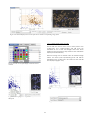
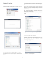
1
User Manual for HoloStudio M4 2.6.2 with HoloMonitor M4 1 2 HoloStudio 2.6.2 Software Manual ©2015 Phase Holographic Imaging AB 3 Contact us: Phase Holographic Imaging Scheelevägen 22 SE-223 63 Lund Sweden +46-(0)46-386080 [email protected] www.phiab.se 4 Introduction to the HoloMonitorTM M4 The HoloMonitorTM M4 is a cell analyzer for adherent cells. It can count cells and analyze adherent cell morphology and confluence. The HoloMonitor TM M4 can also be used for longterm timelapse captures which do not harm the cells. Cells can be tracked through the timelapse capture, both for movement and for morphology. The HoloMonitor TM M4 is incubator proof, allowing for experiments to be performed in a cell culture incubator. Figure 3: The HoloMonitor with a motorized XYZstage Introduction to HoloStudioTM HoloStudioTM is a specially designed software for capture and analysis of digital holographic images with the HoloMonitorTM M4. HoloStudioTM enables the user to capture images both as single captures and as time-lapse captures. Figure 1: The HoloMonitor M4 with a flat sample stage The HoloMonitorTM M4 uses digital holography. This technique is based on measurements of how the cells shift the phase of light that passes through the cells. This kind of live cell imaging does not require any kind of labeling or staining. The procedure is simple: the user captures images of the sample using the HoloMonitorTM M4, and the image is analyzed in the software HoloStudio TM. The imaging procedure does not affect the cells in any measurable way. The cells can be analyzed while growing undisturbed in their usual cell culture vessel. The HoloMonitor TM M4 works with most of the common cell culture vessels such as 6-well plates, petri dishes and IBIDI slides. To simply count cells takes approximately one minute. Confluence measurements are performed simultaneously. To analyze the cells for area, thickness or other parameters, either the built in analysis functions can be used or the data can be exported as xml-files for further work in Excel or similar programs. Cell movement and morphology can be traced over time through a timelapse sequence for both individual cells and for a cell population. The HoloMonitor is equipped with a flat sample stage (Figure 1), which can be replaced with a manual XYstage (Figure 2) or a motorized XYZ-stage (Figure 3). When the M4 is equipped with a motorized stage, samples are directed to move using the computer. The raw data will remain intact, as all changes made by the user only concern how the results are displayed. The changes do not affect the raw data. Applications Some applications have been described in application notes, such as cell motility, cell death, cell cycle and toxicology. The application notes are available on our webpage: http://www.phiab.se/publications/application-notes Figure 2: The manual XY-stage 5 4. View captured images............................................................31 4.1. View an image...............................................................31 4.2. View a timelapse...........................................................31 4.3. View one position of several in a timelapse ................31 4.3.1. Capture pattern timelapse stored in single group..31 4.3.2. Capture pattern timelapse stored in individual groups.............................................................................32 4.4. Move, flip or zoom the cell image ..............................32 4.5. Holographic image display...........................................32 4.5.1. Change the image display.....................................32 4.5.2.Change the image coloring....................................33 4.6. Move, flip or zoom the cell image................................34 4.7. Recalculate a holographic image.................................34 4.7.2. Recalculate the focus manually.............................34 4.7.1. Recalculate the focus automatically .....................34 4.7.3. Recalibrate a holographic image..........................35 4.7.4 Using a background hologram...............................35 Table of Contents Introduction to the HoloMonitorTM M4...................................5 Introduction to HoloStudioTM.............................................5 Applications...........................................................................5 Software Manual...................................................................8 HoloStudio M4 2.6 outline..........................................................9 Main tabs overview...............................................................9 Live Capture..........................................................................9 Analyze Data..........................................................................9 Main Viewing window...........................................................9 Side windows.........................................................................9 Manual PART ONE, Quickguides............................................11 Start up and calibrate the instrument................................12 Time lapse capture..............................................................13 Parallel timelapse captures.................................................14 Cell counting and confluence..............................................15 Proliferation studies ...........................................................16 Morphology analysis...........................................................17 Cell tracking........................................................................18 Data backup.........................................................................19 5. Cell identification...................................................................36 5.1. Identify cells..................................................................36 5.1.1. Select an image.....................................................36 5.1.2. Automatic threshold settings.................................36 5.1.3. Adjust the cell identification..................................37 5.2. Make adjustments for single cells................................37 5.3. Save the cell identification settings..............................38 5.4. Change the image display............................................38 5.5. Image information........................................................39 Manual PART TWO, a user guide............................................20 1. Start up and Close down.......................................................20 1.1. Start up at room temperature......................................20 1.2. Start up in the incubator..............................................20 1.3. Calibration....................................................................20 1.3.1. When everything is well........................................20 1.3.2. If the calibration shows something amiss..............21 1.3.3. If the problems persist...........................................21 1.4. Close down....................................................................21 6. Cell Tracking..........................................................................40 6.1. Start tracking cell movement.......................................40 6.1.1 Add image frames to the analysis...........................40 6.1.2. Select cells to be analyzed.....................................40 6.1.3. Displaying the cell tracking..................................40 6.2. Cell tracking warnings.................................................41 6.3. Adjusting the cell tracking...........................................41 6.3.1. Select the cell to be adjusted.................................41 6.3.2. Switch the tracking from one cell to another.........42 6.3.3. Discontinue a cell tracking...................................42 6.3.4. Continue a discontinued cell tracking...................42 6.3.5. Undo manual changes...........................................42 6.4. Tracking cell morphology............................................42 6.4.1 Display cell morphology parameters for individual cells.................................................................................42 6.4.2 Display different cell morphology parameters.......42 6.5. Export the tracking results..........................................43 2. View live images ....................................................................22 2.1. Focusing .......................................................................22 2.1.1. Automatic versus manual focusing........................22 2.2. Focus a live holographic image using an M4 with a standard sample stage.........................................................23 2.3. Focus a live holographic image using an M4 with a manual XY-stage..................................................................23 2.4. Focus a live holographic image using an M4 with a motorized XYZ-stage..........................................................23 2.4.1. Focus the image semi-automatically.....................23 2.4.2. Focus the image manually.....................................23 2.5. Improve/calibrate the holographic image...................24 2.6. Move the sample stage..................................................24 2.7. Move, flip or zoom the holographic image in the Main Viewing Window..................................................................24 2.8. Change the holographic image display.......................25 2.9. Change the holographic image coloring......................25 7. Analyze and export data........................................................44 7.1. Measure distances directly in the currently viewed image....................................................................................44 7.2. Analyze results in plot..................................................44 7.2.1. Start a new analysis..............................................44 7.2.2. Remove data from plot .........................................45 7.3. Display results in scatter-plot.......................................45 7.3.1. Identify data points as cells ..................................46 7.3.2. Change the scatter-plot axis units.........................47 7.3.3. Change the scatter-plot axis display manually......47 7.3.4. Create, hide and delete plot regions......................47 7.4. Display results in histograms.......................................48 7.4.1. Change the histogram axis units...........................49 7.4.2. Change the histogram X-axis intervals manually. .49 7.4.3. Change the number of bins....................................49 7.5. Export plots and cell data............................................49 7.5.1. Export cell data.....................................................49 7.5.2. Save plots and histograms.....................................50 3. Capture images .....................................................................27 3.1. Store captured images..................................................27 3.2. Capture a single image.................................................27 3.3. Capture a time lapse sequence ....................................27 3.4. Creating a pattern of images to be captured in a sequence...............................................................................27 3.4.1. Select the wells to be captured..............................28 3.4.2. Select positions to be captured..............................28 3.4.3. Create identical capture patterns in all wells........28 3.4.4. Create random capture patterns............................29 3.4.5. Create patterns using the current position............29 3.4.6. Clearing the capture pattern.................................29 3.4.7. Settle time after stage movement...........................29 3.4.8. Capture the pattern...............................................29 3.5. Capture timelapses at several locations in parallel....29 3.5.1. Storing Captured pattern timelapses in one group 30 3.5.2. Storing parallel timelapses in separate groups.....30 8. Cell Count .............................................................................51 8.1. Count cells.....................................................................51 8.2. Adjust the histogram proportions...............................52 8.3. Remove data from plot ................................................52 8.4. Export results................................................................52 6 9. Export images and movies....................................................53 9.1. Add and remove image frames ...................................53 9.2. Edit the images..............................................................53 9.2.1. Zoom, move or flip the image................................54 9.2.2. Adjust the image display.......................................54 9.2.3. Holographic image coloring.................................55 9.3. Create an AVI movie.....................................................55 9.4. Export images...............................................................56 10. Back up.................................................................................57 10.1. Back up of individual projects, groups or frames.....57 10.2. Back up of the entire database...................................57 11. Troubleshooting....................................................................59 11.1. Live Imaging...............................................................59 11.1.1. The Live Capture tab is inactive..........................59 11.1.2. It is impossible to focus the live image................59 11.1.3. The cells are very bright and blurry, showing no inner structures...............................................................59 11.1.4. The cell image is completely white......................59 11.1.5. The cell image is black........................................59 11.1.6. The live image focus was OK, but it slowly turned bad and now it can not be set again................................60 11.2. Capture........................................................................60 11.2.1. The cell image in the Main Viewing window is white...............................................................................60 11.2.2. The capture button is inactive..............................60 11.2.3. In a series of captured images not all images were good................................................................................60 11.3. View Images................................................................60 11.3.1. No image frames are visible in the Image Frame List window.....................................................................60 11.3.2. The cell image in the Main Viewing window is white...............................................................................60 11.4. Cell Identification.......................................................60 11.4.1. No image frames are visible in the Image Frame List window.....................................................................60 11.4.2. The cell image in the Main Viewing window is white...............................................................................60 11.4.3 The automatic cell identification looks strange....60 11.4.4. Some cells are incorrectly segmented as two or more................................................................................60 11.4.5. Two cells are segmented as one...........................60 11.5. Analyze data................................................................61 11.5.1. No image frames are visible in the Image Frame List window.....................................................................61 11.5.2. The cell image in the Main Viewing window is white...............................................................................61 11.5.3. The dots in the dot plot disappeared....................61 11.6. Cell Tracking...............................................................61 11.6.1. The tracks are very irregular...............................61 11.7. Export images and movies..........................................61 11.7.1. No image frames are visible in the Image Frame List window.....................................................................61 11.7.2. The cell image in the Main Viewing window is white...............................................................................61 Addendum A: Morphological parameters...............................62 Holographic microscopy ....................................................62 Holographic technology..................................................62 Phase shift......................................................................62 Threshold settings...........................................................62 Note!...............................................................................62 Cell morphology parameters..............................................63 References............................................................................64 Index.............................................................................................66 7 The Software Manual In the first part of the manual there are quick guides to the most common procedures such as cell counting, timelapse captures and cell tracking. In the second part of the manual, there are detailed guides of how to perform different procedures using HoloStudio, such as how to capture an image and how to analyze the images. The last chapter contains a trouble shooting guide. 8 HoloStudio M4 2.6 outline Information concerning the different side windows can be found by clicking the Information buttons which are placed in the side window headers (Figure 6). Figure 4: The main tabs of HoloStudio 2.6 Main tabs overview HoloStudio M4 Tracking TM is divided into seven functional parts that are represented in seven different tabs (Figures 4 and 5): 1. Live Capture, which concerns the live viewing and capturing of digital hologram images. 2. View Images, which captured images. 3. Identify Cells, which concerns the segmentation of the image, resulting in the identification and outlining of the cells. 4. Track Cells, which concerns the tracking of individual cells through a series of captured frames. 5. Analyze Data, which concerns the analysis of cells in the captured hologram images, as well as display and export of the results. 6. Cell Count, which concerns the counting of adherent cells in their cell culture vessels. 7. Export Images, which concerns the visualization and export of images and movies. concerns viewing The Main Viewing window The Main Viewing window (Figure 5) shows the actual live cell image when the Live Capture tab is open and when the other tabs are open it shows the currently selected stored image. The Side windows Basic functions are found in side windows to the left and right of the Main Viewing window (Figure 5). If the side windows are collapsed they can be expanded by clicking the black arrow tip found in every side window header. Additional functions or parameters are found in the More menus in some of the side windows. These functions are usually not needed for the user but rather for the service engineers. 9 Main tabs Main Viewing window Side windows Figure 5: Overview of a main tab Figure 6: Information button 10 Manual PART ONE Quick guides to commonly used procedures Quick guides index Start up and Calibrate the instrument...........................................12 Time lapse capture and export.....................................................13 Parallel timelapse captures..........................................................14 Cell counting and confluence measurements ..............................15 Proliferation studies ....................................................................16 Morphology analysis...................................................................17 Cell tracking in a timelapse ........................................................18 Data backup.................................................................................19 11 Quick guide: Start up and calibrate the instrument Collect diagnostics 17. If problems persist, collect diagnostics by selecting the Help-option, and then Collect Diagnostics in the top menu. Follow the 1. Putting the instrument in the incubator instructions Put the HoloMonitor M4 in the incubator Wizard. and immediately attach all cords. The instrument must be connected to the wall socket at all times when placed in the incubator. 2. Wait 3-4 hours for the instrument temperature to stabilize. Startup 3. Start the laser 30 minutes prior to use. 4. Start the computer. 5. Start HoloStudio. Calibration at start up 6. Go to the Live Capture tab. 7. The Calibration Wizard window will appear. 8. Follow the instructions of the wizard to perform a calibration. 9. If all values are in the green everything is ready to go. Calibration at other timepoints 10. To calibrate at other timepoints, select the Help-option, and then Calibration wizard in the top menu. 11. Proceed as above. Troubleshooting 12. If any values are in the red, check the following: 13. All cables and connections are correctly attached. 14. There is laser light. 15. The objective and the small laser window are clean. 16. Recalibrate. 12 of the Collect Diagnostics Quick guide: Time lapse capture and movie export Startup 1. Make sure that the instrument has been placed in an incubator for at least three hours while switched on. If the instrument is to be operated at room temperature, start the HoloMonitor 30 minutes prior to use. 2. Start the computer. 3. Start HoloStudio M4. Image capture 4. Go to the Live Capture tab. 5. Choose/create a project and a group. 6. Put the cell sample on a spacer plate or vessel holder of the correct type. Make sure the image is focused. 7. Activate the Timelapse function and enter the total time and the interval between the time points. 8. Press Capture. 9. Use the View Images tab to ensure that the captured imges correspond to your settings. 10. When image capture is complete, proceed to the View Images tab. 11. Run through your images by clicking the Autoscroll button. If needed, recalculate the images. Export individual images or a movie 12. Go to the Export Images tab. 13. Highlight or check the image frames you want to include in the movie or image export. 14. Click the Add buttons in the lower right corner of the program to add the data from the highlighted or checked image frames. 15. Adjust the coloring and viewing angles of the added images. 16. Preview the movie. Export Images or movies. 13 Quick guide: Parallel timelapse captures 1. 16. Export Images or movies. Make sure that the instrument has been placed in an incubator for at least three hours while switched on. If the instrument is to be operated at room temperature, start the HoloMonitor 30 minutes prior to use. 2. Start the computer. 3. Start HoloStudio M4. Image capture 4. Open the Live Capture tab. 5. Put the cell sample on a spacer plate or vessel holder of the correct type. Make sure the image is focused. 6. Choose capture positions in the sample/s. First select a suitable vessel in the Stage positionbox. Find an interesting position for imaging. Click on Remember in the Stage position-box. Repeat for as many positions as required. 7. Create a project and groups for the parallel timelapses. First tick the Capture patterncheckbox in the Capture-box. Then click on Setup storage which will show the Configure destinations-window. Select a project and then tick the Multiple destination groupscheckbox. Click OK. 8. Press Capture. 9. Use the View Images tab to ensure that the captured imges correspond to your settings. 10. When image capture is complete, proceed to the View Images tab. Run through your images by clicking the Autoscroll button. If needed, recalculate the images. Export individual images or a movie 11. Go to the Export Images tab. 12. Highlight or check the image frames you want to include in the movie or image export. 13. Click the Add buttons in the lower right corner of the program to add the data from the highlighted or checked image frames. 14. Adjust the coloring and viewing angles of the added images. 15. Preview the movie. 14 Quick guide: Cell counting measurements images to make sure they are all well and confluence segmented. Note that for cell counting, the cell area identification does not need to be exact, but the cell markers (blue dots) need to 1. Startup be Make sure that the instrument has been measurements the threshold setting needs to placed in an incubator for at least three hours be correct. while switched on. If the instrument is to be correctly placed. For confluence 19. Proceed to the Cell Count tab. operated at room temperature, start the 2. HoloMonitor 30 minutes prior to use. Start the computer. 3. Start HoloStudio. Acquire the cell numbers for one vessel 20. Highlight or check the image frames you want to include in the plot. 21. Click the Add buttons, which are found in the Image capture lower right corner of the window, to add the 4. Go to the Live Capture tab. 5. Choose/create a project and a group. 6. Put the cell sample on a spacer plate or vessel data from the highlighted or checked image frames to the cell count images list. 22. The cell count results are given as “Nbr of cells holder of the correct type. 7. in vessel:” and the confluence results are given as % in the Cell Count Report in the main Select the correct vessel type in the vessel list window. Type the vessel growth area in the in the stage position side window. 8. Ascertain that the live image looks well. 9. Press Capture. text-box below the Cell Count Report window and choose the unit from the scroll bar to obtain a correct cell count/area, or a Vessel 10. Use the View Images tab to ensure that the media captured images correspond to your settings. clicking the Save Report button. again. Continue capturing images until at least five images have been captured. image capture is complete, proceed to the View Images tab. 14. Make sure that the captured images look good. Proceed to the Identify Cells tab. Identify cells 15. Adjust the cell identification in the first image frame using the Adjustments and Manual Changes tabs. 16. Make sure all the images you want to include in the cell count are checked in the Image Frame list on the right side. 17. Click the Apply Checked button, which is found to the bottom right of the window, in order to apply a correct cell 23. Export and save the Cell Count Report by 12. Press Capture. Move the sample and capture the for count/volume. 11. Move the sample. 13. When volume the cell identification adjustments on all the captured images. Alternatively click Apply All. 18. Quickly preview the rest of the checked 15 Quick guide: Proliferation studies correctly placed. For confluence measurements the threshold setting needs to be correct. Startup 1. 18. Proceed to the Cell Count tab. Make sure that the instrument has been placed in an incubator for at least three hours Acquire the cell numbers for one vessel while switched on. If the instrument is to be 19. Highlight or check the image frames you want operated at room temperature, start the to include in the plot. HoloMonitor 30 minutes prior to use. 20. Click the Add buttons, which are found in the 2. Start the computer. lower right corner of the window, to add the 3. Start HoloStudio M4. data from the highlighted or checked image frames to the cell count images list. Image capture 21. The cell count results are given as “Nbr of cells 4. Go to the Live Capture tab. in vessel:” and the confluence results are given 5. Choose/create a project and a group. as % in the Cell Count Report in the main 6. Put the cell sample on a spacer plate or vessel window. Type the vessel growth area in the holder of the correct type. text-box below the Cell Count Report window 7. Ascertain that the live image looks well. and choose the unit from the scroll bar to 8. Press Capture. obtain a correct cell count/area, or a Vessel 9. Use the View Images tab to ensure that the media captured imges correspond to your settings. count/volume. 10. Move the sample. volume for a correct cell 22. Export and save the Cell Count Report by 11. Press Capture. Continue until at least five clicking the Save Report button. images have been captured. 12. When the image capture is complete, Acquire cell numbers for several vessels at proceed to the View Images tab. several time points 13. Make sure that the captured images look 23. Repeat points 6-11 and 12-22 for each cell good. Proceed to the Identify Cells tab. culture vial and for each measuring time point. 24. To compare data from different time points, Identify cells note the cell number and standard deviation 14. Adjust the cell identification in the first image values found in the Cell count report in an frame using the Adjustments and Manual Excel sheet. Changes tabs. 15. Make sure all your images are checked in the Image Frame list on the right side. 16. Click the Apply checked button, which is found to the bottom right of the window, in order to apply the cell identification adjustments on all the captured images. 17. Quickly preview the rest of the images to make sure they are all well segmented. Note that for cell counting, the cell area identification does not need to be exact, but the cell markers (blue dots) need to be 16 Quick guide: Morphology analysis Data analysis using HoloStudio Startup 1. 20. Click New analysis to start a new project. 21. Highlight or check the image frames you want Make sure that the instrument has been to include in the plot. placed in an incubator for at least three hours 22. Click the Add buttons in the lower right corner while switched on. If the instrument is to be of the program to add the data from the operated at room temperature, start the highlighted or checked image frames to the HoloMonitor 30 minutes prior to use. Start the computer. plot. 2. 3. Start HoloStudio. 23. using the X- and Y-axis labels of interest. 24. Image capture Go to the Live Capture tab. 5. Choose/create a project and a group. 6. Put the cell sample on a spacer plate or vessel complete data-set. External data analysis 25. holder of the correct type. the cell data of all added image frames to an in the stage position side window. 8. Ascertain that the live image looks well. 9. Press Capture. xml-file at a location of your choice. 26. 27. captured images correspond to your settings. 11. Move the sample. 12. Press Capture. Move the sample and capture again. Continue capturing images until at least five images have been captured. image capture is complete, proceed to the View Images tab. 14. Make sure that the captured images look good. Proceed to the Identify Cells tab. Identify cells 15. Adjust the cell identification in the first image frame using the Adjustments and Manual Changes tabs. 16. Make sure all your images are checked in the Image Frame List window on the right side. 17. Click the Apply checked button to the bottom right of the program in order to apply the cell identification adjustments on all the captured images. Alternatively, click apply All. 18. Quickly preview the rest of the images to make sure they are all well segmented. 19. Open the data-sheet in a spreadsheet program of choice. 10. Use the View Images tab to ensure that the the Go to the Export tab, below the Main Viewing window. Click the Export data button to save Select the correct vessel type in the vessel list 13. When If necessary, add regions to gain separate data for the included cells, in addition to the 4. 7. Create plots showing the cell morphology by Proceed to the Analyze data tab. 17 Analyze the parameters of interest. Quick guide: Cell tracking in a timelapse to include in the tracking. 22. Click the Add buttons in the lower right corner of the program to add the data from the highlighted or checked image frames. 23. Activate the Add Cells function in the Select Startup 1. Make sure that the instrument has been Mode side window. Add cells to be tracked by placed in an incubator for at least three hours clicking them. 24. Follow the tracking by using the Timeline which while switched on. If the instrument is to be is found below the Cell tracking window. operated at room temperature, start the HoloMonitor 30 minutes prior to use. 2. Start the computer. 3. Start HoloStudio. Spatial tracking 25. Select the Plot Movement tab, which is found behind the Tracking tab. The directions of the cell movements are given in a diagram. Image capture 4. Go to the Live Capture tab. 5. Choose/create a project and a group. 6. Put the cell sample on a spacer plate or vessel Morphological tracking 26. Select the plot Features tab, which is found holder of the correct type. behind the Tracking and Plot Movements tabs. Select the correct vessel type in the vessel list The Area over time is given as a default. To in the stage position side window. view other morphological parameters, select a 8. Ascertain that the live image looks well. different feature in the cell features list which is 9. Press Capture. found below the diagram. 7. 10. Use the View Images tab to ensure that the Export tracking data captured images correspond to your settings. 27. Select the Tracking tab and click export to 11. Move the sample. create an xml-file containing all the tracking 12. Press Capture. Move the sample and capture data. again. Continue capturing images until at 28. The cell tracking image containing the tracks least five images have been captured. complete, can be saved by using the snapshot button in 14. Make sure that the captured images look 29. The spatial tracking diagrams can be exported 13. When the image capture is the Tracking tab. proceed to the View Images tab. by using the Export Plot button in the Plot good. Proceed to the Identify Cells tab. Movement tab. Identify cells 15. Adjust the cell identification in the first image frame using the Adjustments and Manual Changes tabs. 16. Make sure all your images are checked in the Image Frame list on the right side. 17. Click the Apply checked button to the bottom right of the program in order to apply the cell identification adjustments on all the captured images. Alternatively, click Apply All. 18. Quickly preview the rest of the images to make sure they are all well segmented. Adjust the segmentation as needed. 19. Proceed to the Track Cells tab. Track cells through the timelapse 20. Click the button for New Analysis. 21. Highlight or check the image frames you want 18 Quick guide: Data backup Backup of individual projects, groups or frames 1. Click Database in the top menu. 2. Go to Export. 3. When the browser window opens, create a new folder at the selected destination. 4. Select the projects, images or groups that you want to export/back up. 5. Click Export. Backup of the entire database folder 6. Click Database in the top menu. 7. Click Settings. 8. Determine the Root Directory for the database folder HstudioimageDB. This is a road map to find the folder. 9. Go to HstudioimageDB. 10. Copy the entire HstudioimageDB folder. 19 Manual PART TWO A user guide Calibration Wizard window will appear (Figure 7). The wizard can also be accessed from the Help-option in the Top Menu (Figure 8) or from the Calibration side window (Figure 9). When the instructions of the wizard are followed, the instrument will be calibrated. Do this every time the instrument is started or if it has been running for a long time. Chapter 1. Start up and Close down. 1.1. Start up at room temperature • • • Switch on the laser and the instrument. It needs 15 minutes of pre-warming before the laser is stable. Start the computer. Open HoloStudio. Figure 8: The Calibration wizard in the top menu If you want to work with HoloStudio without using the instrument: • • Start the computer. Open HoloStudio. When HoloStudio is not connected to an instrument the Live Capture tab will be inactive. Figure 9: The Calibration wizard in the Calibration side window 1.2. Start up in the incubator • • • • • Put the M4 instrument in the incubator and connect all cords. The electricity must be connected when the instrument is in the incubator, otherwise there will be a condensation problem. Wait 3-4 hours for the instrument temperature to stabilize. Switch on the laser. It needs 15 minutes of pre-warming before the laser is stable. Start the computer. Open HoloStudio. 1.3.1. When everything is well If the calibration is successful, all parameters necessary to achieve good imaging are within their bounds. A window will appear to inform about the successful calibration of objective and background (Figure 10). Thereafter the Calibration Wizard will show the status of three important parameters (Figure 11). Click the Close button to exit from the Calibration Wizard. Values shown to be in the green are excellent, and values in the yellow are acceptable. Figure 7: The Calibration Wizard 1.3. Calibration The first time the Live Capture tab is selected after starting the software with an instrument connected, a Figure 10: The Calibration Wizard showing a successful calibration of objective and background 20 • That the objective and the small laser window are clean, otherwise clean with a cotton swab dipped in ethanol. Then recalibrate using the Recalibrate button (Figure 13). 1.3.3. If the problems persist If problems persist, collect diagnostics by selecting the Help-option, and then Collect Diagnostics in the top menu (Figure 14). Follow the instructions of the Collect Diagnostics Wizard (Figure 15). Figure 11: The Calibration Wizard after a successful calibration 1.3.2. If the calibration shows something amiss If there is a problem with the calibration a warning window will appear (Figure 12). When the OK button has been clicked, a window showing diagnostics values in the red will appear (Figure 13). Figure 14: The Collect Diagnostics Wizard in the top menu Figure 12: The Calibration Warning window Figure 15: The Collect Diagnostics Wizard 1.4. Close down by using the on/off switch on the instrument and by closing the computer program. Figure 13: The Calibration Wizard after an unsuccessful calibration For further information concerning the handling of the HoloMonitor M4, please use the Getting Started guide. If any values are in the red and the calibration could not be performed, check the following: • • • That all cables and connections are correctly attached. That there is laser light. That the blue laser fiber is not pinched down, bent or pulled in any way. 21 Chapter 2. View live images The software focuses the images only when the cell culture vessel is approximately the correct distance from the objective. The aim is to have the cell surface of the cell culture vessel approximately 1 mm above the object tip (Figure 18). Select the Live Capture tab (Figure 16). Below, three holographic phase images are shown that are in focus, out of focus and completely out of focus (Figures 19, 20 and 21). Figure 16: The Live Capture tab 2.1. Focusing There are two different focusing mechanisms that need to cooperate in order for the image to be in focus. With the hardware focus the user places the cells to be viewed at the approximately correct distance from the objective. The software focus describes how well the computer is able to calculate an image based on the light information that reaches the sensor. Figure 19: A holographic phase image that is in focus Put the cell sample on the stage. An image will appear in the Main Viewing window. If the image is correctly focused, the green bar in the Software Focus side window will be in the green area (Figure 17). Figure 17: The Software Focus side window Figure 20: A holographic phase image that is out of focus Figure 21: A holographic phase image that is totally out of focus Figure 18: The suitable distance between the cell culture surface and the tip of the 20x objective. 22 2.1.1. Automatic versus manual focusing 2.4.1. Focus the image semi-automatically Automatic focusing mostly results in well focused images. Some cell samples are more demanding and need to be focused manually. Check Manual in the Software Focus side window (Figure 22). Place the sample on the stage. Wait for the image to stabilize. Make sure that Automatic is activated in the Software Focus side window (Figure 17). Adjust the hardware focus using the Microscope Settings side window (Figure 23) which is found to the right of the Main Viewing window (Figure 5). To the left in the Microscope Settings side window there is an objective representation and a black bar that represents the sample stage (Figure 23). The hardware focus distance can be adjusted in large steps by left clicking, holding and moving the black bar with the mouse cursor. This allows the stage to be moved up and down. The distance between the objective and the sample is shown in the Focus text box. Figure 22: The Software Focus side window To the right in the Microscope Settings side window there is a double gray wheel with red knobs which is used for intermediate (outer wheel) and small (inner wheel) focus adjustment steps. The wheels are moved by left clicking, holding and moving the red knobs. The text box next to the Manual button shows the current software focus distance in mm. That distance can be set to a different value either by entering a value manually or by using the colored slide bar beneath the text box. Move the slide bar until the image looks good. Keep adjusting the focus until the white rectangle in the color bar in the Software Focus side window (Figure17) is placed in the center of the green area of the color bar. The hardware focus is now set to allow the software focus to operate optimally. When using the 20x objective, the aim is to have the cell culture surface 1 mm above the objective tip (Figure 18). 2.2. Focus a live holographic image using an M4 with a standard sample stage Choose the correct spacer plate and put it on the stage. Then put the cell sample on the stage. An image will appear in the Main Viewing window. If the image is correctly focused, the slide bar in the Software Focus side window will be in the green area (Figure 17). The thicker the plate, the further away from the objective the sample will be. Essentially, the image is focused if the correct distance plate is used. If the image is out of focus, try a different distance plate or a different combination of plates until the software focus is in the middle of the green. Figure 23: The Microscope Settings side window 2.3. Focus a live holographic image using an M4 with a manual XY-stage The manual XY-stage is delivered with holders for standard cell culture vessels. If the correct holder is selected, and then the vessel is placed on the stage, the cells will be in focus. 2.4.2. Focus the image manually Automatic focusing mostly results in well focused images. Some cell samples are more demanding and need to be focused manually. Check Manual in the Software Focus side window (Figure 24). 2.4. Focus a live holographic image using an M4 with a motorized XYZ-stage The text box next to the Manual button shows the current software focus distance in mm. That distance can be set to a different value either by entering a The motorized XYZ-stage is delivered with holders for standard cell culture vessels. 23 value manually or by using the colored slide bar beneath the text box. Move the slide bar until the white rectangle is in the middle of the green area. Thereafter the hardware focus has to be adjusted. In the Microscope settings side window there is an image to the left with an objective representation and a black bar that represents the sample stage (Figure 23). The focus distance can be adjusted in large steps by left clicking, holding and moving the black bar with the mouse cursor. This allows the stage to move up and down. The distance between the objective and the sample is shown in the text box. 1. Recalibrate only the image background. Click the Calibrate Background button in the Calibration side window (Figure 25). Remove the sample from the stage and click OK. 2. Use the calibration wizard as described in Chapter 1. Figure 24: The Software Focus side window Figure 26: The Stage Position window The double gray wheel with red knobs in the Microscope settings side window is used for intermediate (outer wheel) and small (inner wheel) focus adjustment steps. The wheels are moved by left clicking, holding and moving the red knobs. 2.6. Move the sample stage The Stage Position window (Figure 26) which is found to the right of the Main Viewing window is used to move the sample stage. As the computer updates the image with small intervals, it is recommended to await the results of one change before making further focus changes. First select the kind of cell culture vessel currently used, by making a selection in the Vessels list. An image of the selected vessel will appear. The blue area represents the area of the vessel available for image capture. In Figure 26, the vessel representation shows microslides. Keep adjusting the hardware focal distance until the cells are in focus. • The stage can be moved in large increments by clicking and dragging the objective representation (i.e. the small double circle) in the Stage Position window. • The stage can be moved in very small increments by using the arrow keys on the numerical pad. • The stage can be moved in intermediary increments by pressing the shift key simultaneously with using the arrow keys on the numerical pad. Figure 25: The Calibration side window 2.5. Improve/calibrate the holographic image Every time the stage is moved the image might need a second or two to stabilize. If the quality of the focused live image is not adequate, it can be calibrated in two different ways. 24 2.7. Move, flip or zoom the holographic image in the Main Viewing Window Different image display options are shown (Figure 27). They can be activated by checking the boxes. Some boxes can be checked in parallel, thus making it possible to combine functions. To zoom the live image, left click the image in the Main Viewing window (Figure 5) and then use the mouse scroll button. • To move the live image to a desired location in the Main Viewing window, click, hold and drag the image using the left mouse button. Checking FFT (Figure 27) displays the Fast Fourier Transform which represents the frequency domains. • To flip and move the live 3-D image, click, hold and drag the image using the right mouse button. Checking Uncut displays the image as it is first reconstructed. • Checking Laser Pattern displays the original interference pattern resulting from the merging of the object and reference laser beams. • Checking Hologram displays the reconstructed image which is based on the laser pattern. The hologram can be displayed showing either the phase or amplitude information of the light wave. • Checking Phase displays the light wave phase information in the hologram. • Checking Amplitude displays the light wave amplitude information in the hologram. • Checking 3-D displays the holographic data as a 3-dimensional representation. • Checking Rotate auto-rotates the image. • Checking Show Ruler displays a horizontal scale bar representative of the distance in X and Y. • Checking Show Color Bar (Figure 27) displays a vertical scale bar representative of the height in Z. • Checking Light Effect applies an artificial light source to the image which may sometimes render an improved image. • Checking Shiny Surface applies an artificial light source to the image which may sometimes render an improved image. Shiny Surface is only visible when Light Effect is checked. 2.8. Change the holographic image display To change how the live holographic image is displayed, open the Viewer Options side window (Figure 27) on the left hand side of the Main Viewing window (Figure 5). Figure 27: The Viewer Options window By clicking the Center button (Figure 28) the image will be centered in the Main Viewing window. Figure 28: The Center button 2.9. Change the holographic image coloring All images originally appear in gray scale. If colors are needed or wanted, use the Coloring side window (Figure 30) to the left of the Main Viewing window (Figure 5). By pressing the Snapshot button an image of the current view will be saved (Figure 29). A set of colors that are saved together is called a Colorset. A previously saved Colorset can be used with the current image by making a selection in the Colorset list which is found at the top of the Coloring side window (Figure 30). Figure 29: The Snapshot button 25 • By left clicking the R-button (Figure 31) the coloring in the image is rescaled to better utilize the optimal dynamic range of the image. This button needs to be operated every time the image coloring is off. • A new color can be added to the colorset by clicking the plus button (Figure 31) and select a new color. A colored triangle representing the new color will appear beneath the histogram (Figure 30). Alternatively, right click on the X-axis and select Add Color. • Change the color by using the right mouse button to click on a colored triangle beneath the histogram and select a new color, alternatively left click the arrow button and select Change Color (Figures 30 and 31). • To change the color span, left click and move the desired colored triangle beneath the histogram using the cursor (Figure 30). • To save a new colorset with the current color settings, left click the arrow button and choose Save As (Figure 31). • To save the current color settings to a previously saved colorset, left click the arrow button and choose Save (Figure 31). Note that this will overwrite the settings previously saved to this colorset. • To delete a colorset, select it in the Colorset list by left clicking it. Then left click the arrow button and select Delete Colorset (Figure 31). Figure 31. Coloring side window functions Figure 30: The Coloring side window 26 3.2. Capture a single image Chapter 3. Capture images Note that only holographic phase representations can be captured! If e.g. an FFT image is desired, please use the snapshot button in the Viewer Options side window (Figures 27 and 29). Put the cell sample on the stage. A live image will appear in the Main Viewing window. Ascertain that you are satisfied with the quality of the live image (See Chapter 2). Click the Capture button. The Capture button is inactive unless a project and a group have been selected (Figure 34). Figure 32: The Live Capture tab 3.1. Store captured images Select the Live Capture tab (Figure 32) Before images can be captured, a place of storage must be prepared. The images must be stored in a Group within a Project. Either open an existing project or create a new project in the Capture window (Figure 33). Then open an existing group or create a new group where the images will be saved. When a new project or group is created, the date and time are automatically included in the name. Figure 35: Activated Timelapse function 3.3. Capture a time lapse sequence To enable slow events to be recorded and studied, a movie can be created from images captured at intervals, i.e. a timelapse movie. In order to capture images for a timelapse study, check the Timelapse box (Figure 35) in the Capture window. Enter the total time for the timelapse and select the desired time unit (seconds, minutes or hours). Enter the interval between the capture time points and select the desired time unit (seconds, minutes or hours). The minimum interval between captures is given to the right of the interval time unit box. Figure 33: The Capture window The number of timepoints will be given when total time and interval are entered. Click the Capture button. 3.4. Creating a pattern of images to be captured in a sequence When it is necessary to capture several images in a sequence, e.g. for cell counting purposes or for parallel timelapses, it is convenient to create a capture Figure 34: The Capture window with an inactive Capture button 27 pattern. When this capture pattern is applied, the instrument automatically captures the set number of images in the set pattern. Check the Capture Pattern box (Figure 36) in the Capture side window. Figure 38: Change vessel type in the Stage position window Figure 36: Activated Capture Pattern function Figure 37: Capture Pattern window showing selected wells Figure 39: Activated Selection function 3.4.1. Select the wells to be captured 3.4.2. Select positions to be captured Click the Selection button (Figure 36). This will make the Capture Pattern window appear, displaying a representation of the currently selected type of cell culture vessel (Figure 37). If necessary, change the current type of vessel in the Stage Position window (Figure 38). Activate the Select Positions button (Figure 39) to select the capture points. Select the capture points by clicking in the well representations. The selected points will be shown as red dots (Figure 40). Even if the selected type of vessel contains only one well, start by activating the Select Wells button (Figure 39) and then click the wells. In the example below (Figure 40), the wells A2 and A3 will be captured, but not A1 and B1-3 as they are not selected. 3.4.3. Create identical capture patterns in all wells To create identical capture patterns in each of several wells, check the box for Identical Patterns in Each Well (Figure 39). Now, every added capture point will appear in all selected wells. 28 3.4.6. Clearing the capture pattern To delete the created pattern click the Clear Pattern button (Figure 39) or the Clear button (Figure 41). To remove single capture points, allow the cursor to hover over a red dot. When a blue + appears, the dot can be removed by right clicking (Figure 42). Pinpointing the dots can be made easier by zooming in the vessel representation in the Capture Pattern window. The image is zoomed in by left clicking in the window and then using the mouse scroll wheel. Figure 40: Selected wells, each displaying a different capture pattern 3.4.4. Create random capture patterns To generate random capture patterns, first fill in the number of capture points in the text box and then click the Generate button (Figure 39). Identical Patterns in Each well and the generation of random capture points can be combined to generate random patterns that are identical in the selected wells. Figure 42: Removing single capture point from a capture pattern 3.4.5. Create patterns using the current position Use the Remember button in the Stage Position side window (Figure 41) to add a capture point located at the current stage position. The current stage position in X/Y as well as Focus is remembered in the Capture pattern. The remembered locations are shown as red dots in the image and if clicked the stage returns to that position. 3.4.7. Settle time after stage movement The function Settle Time After Each Stage Movement (Figure 36) allows medium movement to quiet down after moving the stage to the next capture point. The more the medium moves, the longer settling time is necessary. For a tissue culture flask, 5 seconds are usually enough. 3.4.8. Capture the pattern After setting the Capture Pattern, click the Capture button (Figure 36). Once capture begins with “Capture pattern” selected, the stage will go through the remembered positions one by one and take an image at each location. The Capture Pattern window is closed by clicking the Selection button. 3.5. Capture timelapses at several locations in parallel When combining the Timelapse function and the Capture Pattern function (Figure 43), the set capture pattern will be captured at as many timepoints as are set for the timelapse. Figure 41: Adding a capture point located at the current position to a capture pattern. 29 be sorted into one group for each capture position (Figure 44). The group name can be set to either a new group or to an existing one. The default is to create new groups. There will be an automatic suggestion of the group name, but it is also possible to name the groups manually. It is possible to mix new and existing groups. Click OK to save all groups. In short: 1. Click in the vessel image or use numeric arrow keys to find an interesting position. 2. Click on Remember in the Stage position-box. Every time you click Remember a capture position is saved at the current XYZ-location. 3. Repeat 1-2 for as many positions as required. Tick the Capture pattern-checkbox in the Capture-box. 4. Click on Setup storage which will show the Configure destinations-window. 5. Select a project and then tick the Multiple destination groups-checkbox. 6. Change group names if needed or click OK to accept. The new groups will be created. 7. Select Time lapse in the Capture-box and enter duration and interval. 8. Click Capture. The capturing process will begin and the resulting timelapse images will be stored in the configured groups. Figure 43: A combined timelapse and capture pattern capturing sequence 3.5.1. Storing Captured pattern timelapses in one group By default all captures will be stored in the same group. This becomes impractical if the intention is to capture a time-lapse at each location. Figure 44: The Configure Destination window 3.5.2. Storing parallel timelapses in separate groups When using Capture pattern, the option to create separate groups for each location is available. This is done by clicking on Setup storage (Figure 36) which will show a configuration window (Figure 44). In the Configure Destinations window, deafault is set to adding all captured frames into a single group. When checking Multiple destination groups, the images will 30 4.3. View one position of several in a timelapse Chapter 4. View captured images 4.3.1. Capture pattern timelapse stored in single group In order to view and adjust captured images, select the View Images tab (Figure 45). When a timelapse has been captured at several different positions in parallel using the motorized stage and then stored in a single group, it is possible to view the timelapse for each position separately. The images in the Image Frame List will be arranged in order of capture. If e.g. seven positions have been selected, every seventh frame will belong to the timelapse of that position. Figure 45: The View Images tab 4.1. View an image Start by selecting a Project and a Group in the Image Frame List side window (Figure 46), which is found to the right of the Main Viewing window. Figure 47: The Check function An image frame presentation list for the selected group will appear. Both holographic images and phase contrast images are presented in the list as well as information pertaining to the images. Highlighting an image will make it appear in the Main Viewing window. First highlight the first of the images at the chosen position. Then right click in the Image Frame List, select Check and thereafter Check every X frame (Figure 47). In the above example 7 would then be entered in the Check Frames window (Figure 49). After clicking OK, check the Only Checked option found below the Image Frame List (Figure 48). Now, only the checked images will be displayed when Auto scrolling. Figure 48: The Auto-Scroll button It is possible to select Check frames with comment as an alternative (Figure 47). That allows you to search for a comment such as the particular location XYcoordinate that was saved with the image (Figure 49). Figure 46: The Image Frame List side window 4.2. View a timelapse Start by selecting a Project and a Group in the Image Frame List side window (Figure 46), which is found to the right of the Main Viewing window. Highlight the first frame in the Image Frame List side window. Below the Image Frame list there is an Auto Scroll button (Figure 48). Click that button to show the image frames as a movie. Figure 49: The Check Frames window 31 4.3.2. Capture pattern timelapse stored in individual groups By pressing the Center button (Figure 51) the image will be centered in the Main Viewing window. For each position in the multi-position timelapse, images were stored in a separate group. Go to the group of interest. Highlight the first frame in the Image Frame List side window. Figure 51: The Center button Below the Image Frame list there is an Auto Scroll button (Figure 48). Click that button to show the image frames as a movie. By pressing the Snapshot button (Figure 52) an image of the current view will be saved. 4.4. Move, flip or zoom the cell image To zoom the cell image, click the image in the Main Viewing window and then use the scroll button on the mouse. Figure 52: The Snapshot button To move the cell image to a desired location in the Main Viewing window, click, hold and drag the image using the left mouse button. By checking the boxes different options can be activated. Most boxes can be checked in parallel to combine options. To flip and move a holographic 3-D image, click, hold and drag the image using the right mouse button on the image. • Checking 3-D displays the holographic data as a 3-dimensional representation. • Checking Rotate auto-rotates the image. Rotate is only active when 3-D has been checked. • Checking Show Ruler displays a horizontal scale bar representative of the distance in X and Y. • Checking Show Color bar displays a vertical scale bar representative of the height in Z. • Checking Show Image Info displays additional information associated with the image such as (Figure 53): 4.5. Holographic image display All holographic images will basically appear in gray scale and in 2-D, unless artificial coloring has been chosen and the image display is set to 3-D. Figure 50: The Viewer Options side window for holographic images 4.5.1. Change the image display The holographic image display can be modulated using the Viewer Options window (Figure 50) which is found to the left of the Main Viewing window. • 32 ◦ Project: specifying in which project the image is located. ◦ Group: specifying in which group the image is located. ◦ Nbr: Specifying which number the image has in the group. ◦ Type: Specifying if the image holographic or phase contrast. ◦ Date: specifying the capture date and time of the image. ◦ Width: specifying the image width in μm and pixels. ◦ Height: specifying the image height in μm and pixels. is Checking Light Effect applies an artificial light source to the image which may sometimes render an improved image. • 4.5.2.Change the image coloring Checking Shiny surface applies a change in the surface image display that sometimes renders a better image. Shiny surface is only active when Light Effect is checked. All holographic images will appear in gray scale. Use the Coloring side window (Figure 54), which is found to the left of the Main Viewing window, to add artificial coloring to the images. The colors that are applied will be distributed in the image relatively to the thickness of the objects. A set of colors that are saved together is called a colorset. A previously saved colorset can be used with the current image by making a selection in the Colorset list which is found at the top of the Coloring side window (Figure 54). • By left clicking the R-button (Figure 55) the coloring in the image is rescaled to better utilize the optimal dynamic range of the image. This button needs to be operated every time the image coloring is off. • To add a new color, left click the plus-button (Figure 55) and click Add Color. Select a color. A colored triangle representing the new color will appear beneath the histogram (Figure 54). Alternatively, right click on the X-axis and select Add Color. • Change the color by using the right mouse button to click on a colored triangle beneath the histogram (Figure 54)and select a new color. Alternatively left click the arrow button (Figure 55) and select Change Color. • To change the color span, left click and move the desired colored triangle beneath the histogram (Figure 54) using the cursor. To save the current color settings to a new colorset, left click the arrow button and choose Save As (Figure 55). • To save the current color settings to an already existing colorset, left click the arrow button and click save (Figure 55). Note that this will overwrite the settings previously saved to this colorset. • To delete a colorset, select it in the Colorset list. Then left click the arrow button (Figure 55) and click Delete Colorset. • To save a colorset to an image, left click the arrow button (Figure 55) and choose Apply To followed by Frame. The current colorset will be applied to the currently viewed frame and saved. • To save several images with the current colorset, check the box of the desired images in the Image Frame List side window (Figure 46), left click on the arrow button in the Histogram side window (Figure 55). Choose Apply To followed by left clicking Checked Frames. The current colorset will be applied to the checked image frames and saved. Figure 53: Hologram Image Information Figure 54: The Coloring side window Figure 55: Additional functions found in the Coloring side window 33 Note that changes regarding color will not in any way affect the raw data, and that the original gray-scale image always can be retrieved. 4.7.2. Recalculate the focus manually 4.6. Move, flip or zoom the cell image The text box next to the Manual button shows the software focus distance in mm. The distance can be changed either by entering a value manually or by using the slide bar beneath the text box. After image capture most images are well focused. Some cell samples are more demanding and need to be adjusted manually. Check Manual in the Software Focus side window (Figure 57). To zoom the cell image, click the image in the Main Viewing window and then use the scroll button on the mouse. To determine which focal distance that will result in a well focused image is often a matter of trial and error. To find a starting value, choose an image that was captured at the same time and that is well focused and note the focal distance of that image. To move the cell image to a desired location in the Main Viewing window, click, hold and drag the image using the left mouse button. To flip and move a holographic 3-D image, click, hold and drag the image using the right mouse button on the image. Highlight the image that needs to be recalculated. Select Manual in the Software Focus side window and enter the focal distance of the well focused image in the text box. 4.7. Recalculate a holographic image Click Update. If a holographic image is not correctly focused, as in this example (Figure 56), the software focus can be recalculated after capture in the View Images tab by changing the software calculation settings. If the image focus needs to be improved, enter a new focal distance and click Update. Continue until the image is well focused. Use the arrow button to apply the update to either the current frame or to all checked frames. Figure 56: An unfocused holographic image Figure 58. The Calculation Settings side window set to automatic 4.7.1. Recalculate the focus automatically To replace the manual changes with the original computer focus, Select Automatic in the Software Focus side window (Figure 58) and then click the Update button. If the result is a well focused image, use the arrow button to apply the update to either the current frame or to all checked frames. Figure 57: The Calculation Settings side window set to manual 34 Figure 61: An example of a recalibrated image Figure 59: Example of an incorrectly calibrated image 4.7.3. Recalibrate a holographic image If a captured or imported image is not correctly centered due to aberrant calibration of the instrument, the image will look strange (Figure 59). It can be recalibrated. Clicking the Recalibrate button (Figure 60) in the Software Focus side window will result in a recentered image with an adjusted focal distance (Figure 61). 4.7.4 Using a background hologram The images are noise-improved by using a background hologram to subtract noise from the image. If the background hologram is not correctly set, it might instead disturb the image calculations. There is an option not to use the background hologram (Figure 60). Figure 60: The More list with the Recalibration button and the Use Background Hologram function in the Calculation settings side window 35 Chapter 5. Cell identification 5.1.2. Automatic threshold settings The software will automatically make threshold settings according to the default segmentation method (Figure 64). The base for all image analysis is the cell identification. The software has already made a segmentation suggestion, which might be very good, but it might also need adjustments. The cell number and confluence of each image is immediately given beside the image in the Image Frame List window (Figure 63). Note that the software will suggest a cell identification at the time of capture. This automatic identification needs to be evaluated for each image. Figure 62: The Identify Cells tab Figure 64: Identified cells 5.1. Identify cells Choose the Identify Cells tab (Figure 62). There are several other methods to calculate the threshold settings in the Methods list in the Adjustments window (Figure 65) which is found below the Main Viewing window. 5.1.1. Select an image The Image Frame List side window (Figure 63) is found to the right of the Main Viewing window (Figure 5). Select the project and group where the images are saved (Figure 63). Highlight the image of interest to make it appear in the Main Viewing Window. Figure 65: The Adjustments tab showing the different methods to calculate threshold settings The different threshold settings calculation methods (Figure 65) will result in slightly different cell identifications. It is advisable to try out which method that works best for every type of cell sample. Figure 63: The Frame List side window 36 • Manual allows the user to set the global threshold level using the slider. • Minimum error sets the global threshold level using the minimum error histogram-based threshold method. • Otsu sets the global threshold level using the Otsu method. • Otsu in blocks: the image is split into blocks which are thresholded separately using Otsu method. This is a form of adaptive threshold. • Adaptive mean sets an adaptive thresholding using a mean filter. • Adaptive gaussian sets an thresholding using a gaussian filter. • Double otsu: double thresholding is a method where both a wide and a narrow threshold mask is used. The narrow image is morphologically reconstructed under the wide image. The final image is used as threshold mask. The result is a cleaner threshold mask. The Double Otsu uses double thresholding with Otsu global threshold as mid level threshold. 5.1.3. Adjust the cell identification In the Adjustments window, which is found below the Main Viewing window (Figure 66), the cell identification settings can be adjusted in several ways. In addition to selecting the method to calculate the threshold, as described above, adjustments can be made for each method. The slide bar labeled Adjustment (Figure 66) is used to manually adjust the threshold that is set between cells and background, thus adjusting the area of the segmented cells. adaptive • Double adaptive mean: same as Double Otsu but with two adaptive mean threshold masks. • Double adaptive gaussian: same as Double Otsu but with two adaptive gaussian threshold masks. The slide bar labeled Minimum Object Size (Figure 66) is used to manually adjust the size of the cell core, thus adjusting which identified areas that are cells. • Checking Presmoothing (Figure 66) activates a noise reduction function that will smooth the edges of the cells. • Checking Join Nearby Markers (Figure 66) results in two distinct cell markers being counted as one when they are very close to each other. 5.2. Make adjustments for single cells It is possible to make manual changes to the cell identification for individual cells. It is possible to add, remove and delete as well as enlarge or shrink identified cells. These functions are found in the Manual Changes window (Figure 67) below the Main Viewing window. • Add or Remove (Figure 67) allows the user to add or remove the blue cell markers that identify the cell core. This results in mergers or splits of identified cell areas. • Grow or Shrink allows the user to enlarge or shrink the identified cell regions. • Delete Area allows the user to remove identified cell areas. Figure 66: The Adjustments window Figure 67: The Manual Changes window 37 Several of these functions are also found as a menu when clicking the right mouse button in the image (Figures 68 and 69). To the right in this window there are buttons that enable the user to undo the last adjustment step, to redo the undone step and to clear all adjustments. 5.3. Save the cell identification settings All changes are saved automatically if the box for Auto-apply Changes is checked. This function is found in the Options side window, to the left of the Main Viewing Window (Figure 70). Figure 70: The Options side window If the box is not checked, a warning will appear that the changes are not saved when the user switches from the Identify Cells tab to another main tab (Figure 71). Figure 71: Warning message for changes that have not been saved Figure 68: The adjustments menu when clicking on a cell area Figure 72: The Apply buttons Figure 69: The adjustments menu when clicking outside identified cell areas 5.4. Change the image display In the Options side window (Figure 70), which is found to the left of the Main Viewing window, it is possible to change how the image is displayed. The different display functions can be activated by checking the boxes. The boxes can be checked in parallel, enabling the user to combine functions. Segmentation settings can be applied to a certain frame, to checked frames or to all frames by using the Apply Current, the Apply Checked or the Apply All buttons that are found below the Image Frame List Window (Figure 72). Note that the changes performed using the Manual Changes window (Figure 67) are applied only to individual cells. These changes cannot be applied to other image frames. • 38 Checking Show Threshold displays a red coloring that distinguishes cells from the background. • Checking Show Cell Markers displays a blue coloring that indicates the cell core. • Checking Show Outline displays yellow lines that indicate the border of the cells. • Checking Show Edge Cells Outline displays yellow lines that indicates the border of the cells touching the image edges. • Checking Raw Image causes the image to be displayed as the unadulterated gray scale image • Using Auto-apply Changes allows the user to implement all changes immediately. Figure 73: Information pertaining to a single identified cell 5.5. Image information When the mouse cursor hovers over one of the segmented cells, information concerning that cell will be displayed (Figure 73). • Area is the cell area in m2. • Volume is the optical cell volume in m3. The volume measurements are based on the phase shift of the light and are therefore called “optical”. • Thickness max is the optical thickness of the cell is at its thickest in m. • Thickness avg is the average optical thickness of the cell in m. • Perimeter length is the circumference of the cell in m. • Eccentricity is how elongated the cell is or in how much the cell deviates from being a circle, with 0 corresponding to the perfect circle and 1 being the maximum eccentricity. • Irregularity is how much the circumference of the cell deviates from the circumference of a perfect circle with 0 corresponding to the perfect circumference and 1 being the maximum deviation. 39 Chapter 6. Cell Tracking 6.1.1 Add image frames to the analysis Cells can be tracked through a timelapse sequence and analyzed both for movement and for morphology changes over time. Highlight or check the images to be analyzed, in the Image Frame List to the right. Click the appropriate Add button (Figure 77). The Add buttons are found below the Image Frame List. The added image frames will be shown in the Source Frames window (Figure 78) below the Cell Tracking window (Figure 91). 6.1.2. Select cells to be analyzed In order to follow a cell through a timelapse, the cell needs to be added. Go to the Select Mode side window (Figure 79), and activate Add Cells. Figure 74: The Cell Tracking tab 6.1. Start tracking cell movement Go to the Cell Tracking tab (Fig 74). A window will appear where a new analysis or a stored analysis can be selected (Figure 75). Figure 79: The Select Mode side window In the Cell Tracking window, the center of each identified cell is marked with a small orange + (Figure 80). If the identification is not satisfying, go to the Identify Cells tab, and adjust the cell identification (Chapter 5). Click each cell to be followed (Figure 80). The cell will be followed from the frame where it is added. Figure 75: The Select Analysis buttons After clicking the New Analysis button a text will appear which says that frames must be added in order to analyze images for cell tracking (Figure76). Figure 76: The Cell Tracking instruction text Figure 80: Clicking to add a cell to the tracking results 6.1.3. Displaying the cell tracking There is a Timeline below the Cell Tracking window (Figure 81). By moving the small gray slider, the image frame sequence will be played through. The tracks showing the cell movements movement will then be displayed (Figure 82). Figure 77: The Add buttons Figure 78: The Source Frames window 40 Figure 81: Timeline for cell tracking Figure 84: The warning in the segmentation for the previous, current and next image frame. 6.3. Adjusting the cell tracking Figure 82: Tracks showing cell movements Sometimes the software will track the wrong cell, e.g. when cells are moving very close to each other and then separate again. This needs to be adjusted manually. The movements can also be seen in the Plot Movement tab, which is found behind the cell tracking window. Note that the adjustments will be active from the frame of adjustment and forwards through the timelapse. 6.2. Cell tracking warnings When the cell tracking for some reason is deviating from the previous image, the software will give warnings. The warnings are listed in the Warnings tab (Figure 83), which is found below the Timeline. When the Show button is clicked (Figure 83), a window opens which displays the previous, current and next segmentation of the cell (Figure 84). It is then possible to see if the warning is appropriate or if it can be ignored. If the warning is caused by a normal cellular event such as cell division, the Ignore box can be checked and the warning is then ignored (Figure 83). In the example (Figure 84) the segmentation needs adjusting, and the user would then click Identify to go to the cell identification tab. Figure 85: Changing the cell tracking 6.3.1. Select the cell to be adjusted Activate Select in the Select Mode side window (Figure 79). Click on the cell to be adjusted. A new set of functions will then be available in the Change Tracking side window (Figure 85). The cell that will be adjusted is noted in the Change Tracking side window. Figure 83: The Warnings tab 41 6.3.2. Switch the tracking from one cell to another 6.3.5. Undo manual changes After selecting the cell to be changed, click the Modify Location button in the Change Tracking side window. Then click the cell that actually should be followed instead of the selected cell. Now, the colored border is transferred to the new cell to be followed (Figure 86). The software will recalculate the tracking automatically from the present image frame and forward through the time lapse. If the manual changes need to be undone, start by selecting a cell. Then click either the Undo for this Frame, or the Undo for all Frames button (Figure 85). When clicking Undo for this Frame, the manual change in the current frame will be undone, and the tracking will be recalculated according to the change in settings. When clicking Undo for all Frames, the manual changes in all frames will be removed and the tracking will be recalculated according to the change in settings. 6.4. Tracking cell morphology Once the cell movement has been tracked, the cell morphology can also be followed over time by using the Plot Features tab (Figure 88). Figure 86: Transfer the tracking from one cell to another. The left image shows the selected cells, and the right image shows how the tracking is transferred. 6.3.3. Discontinue a cell tracking Sometimes a tracking needs to be discontinued, e.g. when a cell leaves the image area. After selecting the cell to be changed, click the Unset button in the Change Tracking side window (Figure ). The tracking will be discontinued from the present frame. Figure 88: The Cell Morphology Tracking tab A new button, Set location, will appear in the Change Tracking window (Figure 87). 6.4.1 Display cell morphology parameters for individual cells By checking or unchecking the colored boxes displayed beside each cell name, morphological parameters are shown for that cell. Black always shows the average of the cell population. Figure 89: Switching cell features Figure 87: Set Location 6.4.2 Display different cell morphology parameters 6.3.4. Continue a discontinued cell tracking By using the Cell Feature function found below the diagram (Figure 89) different morphological parameters can be displayed. The list contains all parameters as well as distance and speed of movement. For a full list of parameters, go to Addendum A. When a cell has been unset it will still be present in the Tracked Cells list, but noted as not present. In order to resume the tracking in a different frame, select the cell in the Tracked Cells list and click the Set location button (Figure 87). Then click the cell in the frame where the tracking should be resumed. 42 Figure 90: Track and Export buttons found to the right of the Cell Tracking window in the Tracking tab 6.5. Export the tracking results The raw data can be exported into an xml-file by clicking the Export button (Figure 104) which is found in the Tracking tab. The xml-file can be imported into e.g. Xcel. The image currently displayed in the cell tracking window can be saved by clicking the Save button, found below the Cell Tracking window (Figure 91), which is found in the Tracking tab. Figure 91: The Save button which is found below the Cell Tracking window 43 Chapter 7. Analyze and export data Click the Measure button in the Viewer Options side window (Figure 93) to make manual measurements of objects in the current image. When the measuring function is activated, the measurement is started by left clicking anywhere in the image. The measurement is finished by left clicking at a new point in the image. The main part of the cell data analysis is performed in the Analyze Data tab that contains tools for analyzing the identified cells. A simple tool for measuring distances or objects in a currently viewed image is found in the View Images tab. The measured distance is shown with a blue bar (Figure 94). A window displaying the results appear to the bottom right of the main viewing window. The results include a profile of the measured object. The data are saved as an image when the Snapshot button (Figure 95) in the Viewer Options window is clicked. 7.1. Measure distances directly in the currently viewed image Choose the View Images tab (Figure 92). Figure 95: The Snapshot button It is possible to move the image in the Main Viewing window while the measuring function is activated. The image is moved by clicking and dragging. Figure 92: The View Images tab When the Measure button is clicked again, the measuring function is deactivated. 7.2. Analyze results in plot 7.2.1. Start a new analysis Choose the Analyze Data tab (Figure 96). Figure 93: The Viewer Options side window for holographic images Figure 96: The analyze data tab A window will appear where a new analysis or a stored analysis can be selected (Figure 97). Figure 97: The Select Analysis buttons Figure 94: The blue measuring bar and the results window After clicking the New Analysis button a new message will appear (Figure 98). 44 If several images are added to the plot, the data from all images will be displayed in the same plot unless the Only Current Frame (Figure 102) is checked. Then only the data from the current frame are displayed. The Only Current Frame function is found below the Scatter-plot. Figure 98: The Add message Select a Project and a Group in the Image Frame list window (Figure 99), which is found to the right of the Main Viewing window (Figure 5). Figure 102: The Only Current Frames function 7.2.2. Remove data from plot To remove data belonging to a single frame from a plot, highlight that frame in the Source Frames list (Figure 101). Then use the remove button that is found above and to the right of the Source Frames list (Figures 101 and 103). Figure 99: The Image Frame list Figure 103: The Remove from Plot buttons To add data, highlight image/s and transfer to the plot by using the Add Selected button (Figure 100), which is found below the Image Frame list window. Several images can be added simultaneously if they are all highlighted. The shift key can be used to highlight several consecutive images and the ctrl key to highlight non-consecutive images. 7.3. Display results in scatter-plot The cell morphology data are first represented as a scatter-plot, with the segmented cell images displayed beside the plot (Figure Fel: Det gick inte att hitta referenskällan). The data point for each cell is represented as a colored box. If several frames are represented in the plot, the data points from all images will be displayed in the plot simultaneously, while the cell image window shows the frame that is highlighted in the Source Frames tab. Figure 100: The Add buttons below the Image Frame list The images that are included in the analysis are shown in the Source Frames tab (Figure 101) which is found below the Main Viewing window. The data points will be displayed in the plot with the color shown in the color box in the Source Frames tab (Figure 105), which is found below the Scatter-plot tab. To change the display color, left-click the color box for the added frame and select a different color. Figure 101: The Source Frames tab which is found below the Scatter-plot tab 45 Figure 104: Results displayed in a scatter plot shown with the corresponding image frame 7.3.1. Identify data points as cells Hover with the mouse cursor over a data point in the scatter-plot. The corresponding cell will then be identified in one of the cell images that have been added to the plot (Figure 106). Data for that cell will be displayed simultaneously. When hovering over a certain cell in an added image frame, the data point representing that cell will be identified in the scatter-plot, and data for that cell will be displayed (Figure 107). Figure 105: The several plot display colors that can be selected Figure 107: Identifying the data point representing a certain cell Figure 106: Identifying the cell represented by a certain data point Figure 108: The X- and Y-axis labels 46 7.3.2. Change the scatter-plot axis units The axis labels of the scatter-plot can be changed by using the listed X- and Y-axis parameters found below the scatter plot (Figure 108). For a full list of axis label parameters, go to Addendum A. 7.3.3. Change the scatter-plot axis display manually Figure 112: A list of region types The Plot Area settings (Figure 109) are found below the Scatter-plot. The area of the scatter-plot (i.e. the values of the X- and Y-axis) is set automatically to fit in all values from all added frames. In both cases a list of region types appears (Figure 112). Select a region type by clicking it. Then click in the plot where the region setting should begin. To set the plot area manually, deactivate Auto-scale by unchecking the box (Figure 109) and then entering the desired X and Y minimum and maximum values (Figure 110). For the linear region and the X- and Y- axis regions the second click in the plot determines where the region ends. For the arbitrary region, every click in the plot will add to the region. Finish the region by clicking the starting point again. The starting point will expand to indicate that the region is closed. If clicking the region does not make it “stick”, try clicking a little slower. Figure 109: The Plot Area settings Figure 110: The Fixed Plot Area window Alternatively, the plot area can be changed with the mouse scroll button. Left click in the plot and scroll using the mouse scroll button. To move the plot area in the scatter-plot, left click in the plot, hold and drag. • X-axis region, where X-axis values are the region cut off values (Figure 113). • Y-axis region, where Y-axis values are the region cut off values (Figure 113). • Linear region, where clicking in the diagram window results in straight lines that cut off the region from origin (Figure 114). • Arbitrary region, where repeated clicking in the diagram window results in an irregular figure that outlines the region. To finish the region, close it off by clicking in the starting point (Figure 114). The regions are summarized in the Regions tab (Figure 115), which is found below the Scatter-plot tab. Regions can be hidden by unchecking the Display box. 7.3.4. Create, hide and delete plot regions The scatter-plot diagram can be divided into regions to separate out data from certain cells or cell populations. When clicking the right mouse button while hovering over the plot, a menu will open. When Define New Region is selected, a region menu will appear (Figure 112). Alternatively there is an Define Region button (Figure 111) below the Scatter-plot tab, to the right of the Auto-scale function. Regions can be deleted by highlighting the region in the Regions window and then clicking Delete, which is found to the upper right in the regions tab (Figure 116). Figure 111: The Define Region button 47 7.4. Display results in histograms The results can also be displayed as histograms, where one cell parameter is offset against the cell number (Figures 117 and 118). Figure 113: An X-axis region (green) and a Y-axis region (blue) Figure 117. The Histogram tab Figure 118. A Histogram When Only Current Frame (Figure 119) is checked, the data from each frame is displayed when the corresponding image is highlighted in the Source Frames tab (Figure 120) below the Scatter Plot tab. Figure 114: A linear region (blue) and an arbitrary region (green) Figure 119: The Only Current Frame button Figure 115: The Regions tab The data from each image frame will be represented in the histogram with the color shown in the color box in the Added Frames window. To change the display color, left-click the color box beside the frame number in the Source Frames tab and select a different color (Figure 121). Figure 116: The Delete buttons 48 To set the histogram X-axis interval manually, Autosettings must be unchecked (Figure 124). Enter the minimum and maximum values. 7.4.3. Change the number of bins Figure 120: The Source Frames tab The number of bins in the histogram is set automatically. To set the number of bins manually, uncheck the Auto settings (Figure 124), which is found below the Histogram. By adjusting the slide bar, few (Figure 125) or several bins (Figure 126) can be displayed in the histogram. Figure 121: Color options for histogram data display 7.4.1. Change the histogram axis units The X-axis label of the histogram can be changed by using the Cell feature list below the Histogram (Figure 122). A list of x-axis label parameters are found in Addendum A. Figure 125: A histogram with few bins Figure 122: The Histogram X-axis label 7.4.2. Change the histogram X-axis intervals manually Figure 126: A histogram with several bins The histogram X-axis interval is set automatically (Figure 123) to fit in all values from all added frames. Figure 123: The Auto-Setting function Figure 127: A histogram with several bins Figure 124: Making the settings manually 49 7.5. Export plots and cell data Alternatively, plots and histograms can be saved by right clicking the diagrams and then choose Save. In the Export tab (Figure 128), cell data from the current plot can be exported to an XML-file. The xmlfile can be imported into e.g. Xcel. Images of the current plot and histogram can be saved as bitmap, GIF, JPEG, PNG or TIFF by using the Save buttons (Figure 129). 7.5.1. Export cell data The Export tab is found below the Scatter-plot(Figure 128). By clicking the buttons, cell data can be exported to XML or ICE files. Figure 128: The Export tab Click the Export buttons to export all cell data. A browser window will open . The file will automatically be named with date and a code, but it is possible to rename the file. Save the file to an appropriate place. In this step, all data pertaining to the image frames added to the current plot are exported. Figure 129: The Save Plot and Histogram buttons 7.5.2. Save plots and histograms The Save Plot and Save Histogram buttons are found below the Scatter-plot and the Histogram. Click the Save Plot button (Figure 129). A browser window will open. The file will automatically be named Scatter Plot, but it is possible to rename the file. Decide which image format you want. Save the file to an appropriate place. 50 Chapter 8. Cell Count Fill in the correct cell culture vessel growth area and the volume of the cell culture vessel medium content in the text boxes below the Cell Count Report (Figure 134). Cells are counted and analyzed for confluence, cell area and volume in the Cell Count tab. Figure 134: Text boxes for cell culture vessel area and volume Figure 130: The Cell Count tab The images are then analyzed, and the results are presented in a Cell Count Report (Figure 135). 8.1. Count cells Choose the Cell Count tab (Figure 130). A text will appear which says that five image frames or more must be added in order to analyze images for cell count, confluence, cell area and volume (Figure 131). Figure 135: The Cell Count Report Figure 131: The Cell Count instruction text The report contains data on: Highlight or check the images to be analyzed, in the Image Frame List to the right. Click the appropriate Add button (Figure 132). The Add buttons are found below the Image Frame List. The added image frames will be shown in the Source Frames window below the Cell Count Report (Figure 133). Figure 132: The Add buttons • Number of cells in the vessel. • Number of cells per ml. • Confluence. • Report date. • Capture time points. • Vessel growth area. • Vessel media volume. • • Total number of image frames used for the analysis. The total area of the images. • The total number of cells in the images. • The number of cells that are placed on the image edge, and which therefore are not included in the morphological analysis, although they are included in the cell count. Of the edge cells 50% are included in the the cell number while 50% are not included. If the confidence interval is too large (larger than 1015%) more images should be added to the analysis. The more unevenly the cells grow, the more images are needed for the cell count. Figure 133: The Source Frames window 51 Figure 136: The histogram adjustment functions 8.2. Adjust the histogram proportions The X-axis of the Area and Volume histograms can be set either automatically, or manually. For each axis the lowest and the highest value can be set as well as the number of bins that present the data. The adjustment text boxes are found below the cell count report window (Fig. 136). 8.3. Remove data from plot To clear the plot from all data from all image frames, use the Remove All command, which is found with an X to the right in the Source Frames window (Figure 137). To remove data belonging to a single frame from a plot, highlight that frame in the Source Frames window and then use the Remove Highlighted command, which is found with an X to the right in the Source Frames window (Figure 137). Figure 137: The Remove functions 8.4. Export results Below the Cell Count Report there is a Save report button (Figure 138). Clicking the button generates a pdf containing all relevant data, including the area and volume as histograms and a list of the included image frames. When the boxes are un-checked, histograms and frame list can be excluded from the report. Figure 138: The Save Report button 52 Chapter 9. Export images and movies 9.1. Add and remove image frames In the Export Images tab, image frames can be edited and exported either as individual images in several standard formats or as AVI movies (Figure 139). Below the Image Frame list (Figure 140) there are buttons to add image frames to the Main Window. The side windows become active only when one or several images have been added. By clicking the Add Highlighted button (Figure 140) which is found below the Image Frame list, the data from a single image frame or from several frames can be added when the frames are highlighted in the Image Frame list. The shift key can be used to highlight several consecutive images and the ctrl key to highlight non-consecutive images. Figure 139: The Export Images tab Alternatively, the box to the left of each image can be checked and then the Add Checked button is clicked. All image frames can be added by clicking the Add All button. Clicking the Remove buttons (Figure 141) will remove either only the highlighted or all of the added images. Figure 141: The Remove buttons The Main Viewing Window contains a view of the currently active added image as well as thumb nails of all the added images (Figure 142). By clicking a thumb nail a new image will be displayed in the Main Viewing window. Figure 142: The Main Viewing window Figure 140: The Image Frame list 53 9.2. Edit the images 9.2.1. Zoom, move or flip the image The Perspective side window (Figure 143) shows how the image has been moved, flipped or zoomed. To zoom, left click the cell image in the Main Viewing window and then use the mouse scroll button. To move the image to a desired location in the Main Viewing window, click, hold and drag using the left mouse button. To flip and move the 3-D image, click, hold and drag using the right mouse button. Figure 145: The Background color setting 9.2.2. Adjust the image display The Viewer Options side window (Figure 144), which is found to the left of the Main Viewing window, is used to adjust the image display. Some of the options are inactive when a phase contrast image is viewed. Figure 143: The Perspective side window Click one of the Use-buttons to apply the changes to the added images that are highlighted or to all added images. • Checking 3-D displays the image as a 3dimensional representation. • Checking Show Ruler displays a horizontal scale bar representative of the distance in X and Y. • Checking Show Color Bar displays a vertical scale bar representative of the height in Z. • Checking Show Image Info displays additional information associated with the image such as: ◦ First row: specifies in which project the image is located. ◦ Second row: specifies in which group the image is located. ◦ Nbr: specifies which number the image has in the group. ◦ Type: specifies if the image is holographic or phase contrast. ◦ Date: specifies the capture date and time of the image. Figure 144: Viewer Options side window • 54 Checking Light Effect applies an artificial light source to the image which may sometimes render an improved image. • Checking Shiny surface applies a change in the surface image display that sometimes renders a better image. Shiny surface is only active when Light Effect is checked. • To change the Background color, left click the Background color box and select a new color (Figure 145). color. A colored triangle representing the new color will appear beneath the histogram (Figure 146). Alternatively, right click the x-axis at the position where a new color is wanted and select Add Color from the menu that appears. 9.2.3. Holographic image coloring Adjust the holographic image color display and the image dynamics with the Coloring side window (Figure 146). A set of colors that are saved together is called a colorset. A previously saved colorset can be used with the current image by making a selection in the Colorset list which is found at the top of the Coloring side window (Figure 146). Click one of the Use-buttons to apply the changes to the added images that are highlighted or to all added images. • Change the color by using the right mouse button to click on a colored triangle beneath the histogram and select a new color, alternatively left click the arrow button and select Change Color (Figures 146 and 147). • To change the color span, left click and move the desired colored triangle beneath the histogram using the cursor (Figure 146). • To save a new colorset with the current color settings, left click the arrow button and choose Save As (Figure 147). • To save the current color settings to a previously saved colorset, left click the arrow button and choose Save (Figure 147). Note that this will overwrite the settings previously saved to this colorset. Figure 147: Additional functions found in the Coloring side window 9.3. Create an AVI movie Figure 146: The Coloring side window When the set of images look good, click the Use For All-buttons in both the Perspective side window and the Coloring side window (Figures 143 and 146). Preview the movie by clicking the preview button Play (Figure 148). The number of slides per second are not shown as in the finished movie, but rather at a set speed. Additional functions are found as buttons and in a menu which is found at the arrow tip (Figure147). • By left clicking the R-button (Figure 147) the coloring in the image is rescaled to better utilize the optimal dynamic range of the image. Note that this button needs to be operated every time the image coloring is off. • To add a new color to the colorset, left click the plus button (Figure 147) and select a new 55 Figure 148: The Preview side window If the preview looks good, click the Export Movie button in the Export window (Figure 149). Figure 151: The Export Images side window Figure 149: The Export window Clicking the Export Movie button will open an export window (Figure 150). Select the destination folder by browsing. By moving the slide bar it is possible to set the number of frames per second that will be shown in the AVI movie. Figure 150: The Export Movie side window 9.4. Export images When the image has been set up nicely and looks good, click the Export Images button to open an export window (Figure 151). Select the destination folder by browsing. Check the box to add frame comments to the file name. The Image format can be selected in the drop menu. When the box for Use Plain Image Images is checked, no coloring or 3-D will be displayed in the exported image. When the box for Transparent Background is checked, the images will be exported without background. 56 Chapter 10. Back up A browser window will open (Figure 153). Click Browse. Create a new folder at the selected destination (Figure 154). In order to make a safety back up of your data you need to either export or copy the database. When a folder has been created, a window displaying the groups and projects will appear (Figure 155). Select the projects, groups or images that you want to export/back up. Click Export. Alla database information will now be copied to the created folder. In order to access the data in the folder, the data must be imported into the software again using Database Import. Figure 152: The Database menu Figure 153: The Browser window Figure 155: Select projects, groups or images for export 10.2. Back up of the entire database First locate the database. Click Database in the top menu (Figure 152). Then click Settings. Determine the Root Directory for the database folder HstudioimageDB (Figure 156). Figure 154: Create new folder 10.1. Back up of individual projects, groups or frames Figure 156: Database settings information containing the root directory of HstudioimageDB Click Database in the top menu (Figure 152). Then click Export. 57 Find HstudioimageDB on the computer hard drive (Figures 157 and 158). Note that the root directory is different for different computers. Copy the entire HstudioimageDB folder. In order to access the data in the folder, HoloStudio must be directed to use the copied data base. Figure 157: The pathway to the PHI folder Figure 158: The PHI folder that contains the HstudioimageDB database 58 Chapter 11. Troubleshooting adequate. When auto-exposure is on (camera properties window in the left side window), the exposure time should be less than 10 ms. If the exposure time is long, start by checking that the laser unit is connected properly both to power and to the instrument. If the laser is connected properly and the exposure time still is very long, please contact instrument service. 11.1. Live Imaging 11.1.1. The Live Capture tab is inactive Why? The software cannot find the HoloMonitor. Fix: Check that the USB- and power cables are properly connected. Try restarting HoloStudio. Why? The objective and the laser window need cleaning. Fix: Clean with an ethanol-soaked Q-tip and dry after with a dry Q-tip. (http://www.phiab.se/support/contact, use the cleaning movie) Why? The drivers are corrupt. Fix: Start the Windows Device Manager and check for any drivers with exclamation marks. Try disconnecting the USB-cable from the instrument and connect it again and wait a couple of minutes. If the problem persists, try to run the installation program again. The driver files are located under C:\PHI\Drivers as subfolders. If a driver has an exclamation mark shown in device manager it may be possible to re-install it by right-clicking in device manager and selecting Update driver. Then browse to driver folder under C:\PHI\Drivers. Why? If the cells are very thin or very sparsely distributed in the vessel, the auto focus has difficulties to find focus. Fix: Set the software focus manually instead of automatically. Activate the manual focus mode by clicking the Manual button in the Software Focus side window in the Live Capture tab. Thereafter drag the slider to the green area in the focus bar, and then adjust the hardware focus. Thin cells have a very narrow focal distance and focusing has to be performed with great care. 11.1.2. It is impossible to focus the live image Why? For M4 with distance plates, the wrong distance plate might be used. Fix: Make sure that the correct spacer plate or vessel holder for that cell culture vessel is used. The bottom of the vessel (where the cells are) should be approximately 1 mm from the objective. Vessels with a thick bottom or a high socket need the thinnest spacer plate. Vessels or slides which are thin should be put on the thickest or medium thick distance plate. Why? The instrument was not switched on for 30 minutes before use at room temperature or put in an incubator at least three hours before use. If the instrument is warming up, the focus will change all the time and the focus settings will need to be adjusted continuously. Fix: Allow the instrument the warming up period. Why? Something causes the instrument to vibrate. Fix: Check that the cables connected to the M4 are slack and not touching anything. Ensure that no vibrations come from sources like centrifuges or hard working air vents. Why? The cell culture vial is scratched or smudged. Fix: Even wiping the cell culture vessel clean will probably not help much as traces of dirt will still persist. Instead, avoid touching the top and bottom surfaces of the cell culture vessel when handling it, even when wearing gloves. Avoid anything that might scratch the surfaces. Cell culture plastic is very easily scratched. 11.1.3. The cells are very bright and blurry, showing no inner structures Why? There is condensation on the inside of the cell culture vessel. Fix 1: If the cell culture vessel is a flask, tighten the cap and gently rinse the condensation away with the cell culture medium. Avoid getting medium into the cap. If the cell culture vessel is a multiwell plate or a petri dish, allow the vessel to reach room temperature, alternatively switch lids to a new lid or try working without a lid. NOTE! Working without the lid is a nonsterile procedure! Fix 2: If the cell culture medium is replaced with cold PBS or cold cell culture medium immediately after taking the multi well plates and petri dishes from the incubator, there will not be condensation. Replace the PBS with medium again after the analysis. Why?: The image dynamics are not optimally set. Fix: Press the R-button by the histogram in the Coloring side window. 11.1.4. The cell image is completely white Why?: The image dynamics are not optimally set. Fix: Press the R-button by the histogram in the Coloring side window. 11.1.5. The cell image is black Why? The laser unit is not switched on or connected properly. Fix: Start by checking that the laser unit is connected properly both to power and to the instrument. If the Why? The laser intensity is not optimal for the chosen cell sample. Fix: Make sure that the laser beam intensity is 59 laser is connected properly and the image still is black, please contact instrument service be visible. Fix: Uncheck the Only Checked box. Why? The images are either zoomed in or out to much. Fix: Use the mouse scroll to scroll back. 11.3.2. The cell image in the Main Viewing window is white Why? The image dynamics are not optimally set. Fix: Press the R-button by the histogram in the Histogram side window. Why? The image dynamics are not optimal. Fix: Click the R-button in the Histogram side window. 11.4. Cell Identification 11.1.6. The live image focus was OK, but it slowly turned bad and now it can not be set again 11.4.1. No image frames are visible in the Image Frame List window Why? There is probably a drop of water hanging from the top/lid of the cell culture vessel. As the drop grows larger it will increasingly disturb the image focus. Fix: Gently tilt the cell culture vessel and make the drop slide to the side of the vessel. Why? No Project and Group has been selected. Fix: Select a Project and a Group. Why? If the Only Checked box is checked, only checked images will be displayed. If no image frames in the current Group has been checked, no frames will be visible. Fix: Uncheck the Only Checked box. 11.2. Capture 11.2.1. The cell image in the Main Viewing window is white 11.4.2. The cell image in the Main Viewing window is white Why? The image dynamics are not optimal. Fix: Click the R-button in the Histogram side window. Save by clicking the arrow button and then Apply To, and then Frame. Why? The image dynamics is not optimal. Fix: Click the R-button in the Histogram side window. 11.4.3 The automatic cell identification looks strange Why? The chosen threshold setting method might not suit the cells. Fix: Try a different threshold setting method. 11.2.2. The capture button is inactive Why? The capture button is inactive when no project and group has been selected. The program then does not know where to store the captured images. Fix: Select or create a Project and a Group. Why? If the cells grow at a very high density, the threshold setting methods are not able to identify individual cells. If cells are growing very closely they cannot be separated out. Fix: Adjust the threshold setting using the Adjustment slide bar. Make sure that only the background and not any cells are defined as background. Then use the confluency or the cell dry mass parameter to determine the amount of cells instead of the cell number. 11.2.3. In a series of captured images not all images were good Why? There might have been a scratch or a smudge on the vessel where the bad images were captured. Fix: Capture extra images and then discard the bad ones. Why? There is background noise in the image that causes the background to be set at an incorrect level. Fix 1: Make sure that background and laser are calibrated prior to analysis. Fix 2: Capture extra images and then discard the bad ones. Why? Floating cells disturbed the automatic software focus. Fix: Follow the instructions in section 4.5. to recalculate the software focus. 11.3. View Images 11.3.1. No image frames are visible in the Image Frame List window 11.4.4. Some cells are incorrectly segmented as two or more Why? No Project and Group has been selected. Fix: Select a Project and a Group. Why? The minimum object size is set too low. Fix: Adjust the Min object size using the slider in the Object definition box under the Adjustment tab so that each cell has one blue marker. Why? If the Only Checked box is checked, only checked images will be displayed. If no image frames in the current Group has been checked, no frames will 60 11.4.5. Two cells are segmented as one 11.7.2. The cell image in the Main Viewing window is white. Why? The minimum object size is set too high. Fix: Adjust the Min object size using the slider in the Object definition box under the Adjustment tab so that each cell has one blue marker. Why? The image dynamics is not optimal. Fix: Click the R-button in the Histogram side window. Why? The cell confluency is very high and the cells are difficult to separate out. Fix: Separate the two cells by using the Add or remove button under the Manual changes tab in the Identify cells tab. 11.5. Analyze data 11.5.1. No image frames are visible in the Image Frame List window Why? No Project and Group has been selected. Fix: Select a Project and a Group. Why? If the Only Checked box is checked, only checked images will be displayed. If no image frames in the current Group has been checked, no frames will be visible. Fix: Uncheck the Only Checked box. 11.5.2. The cell image in the Main Viewing window is white. Why? The image dynamics is not optimal. Fix: Click the R-button in the Histogram side window. 11.5.3. The dots in the dot plot disappeared Why? The changes in settings and display has caused the dots to be outside the range of the plot values. Fix: Set the plot area to Automatic and click the Reset View button. 11.6. Cell Tracking 11.6.1. The tracks are very irregular Why? The cell segmentation is not properly done. Fix: Go to the Identify Cells tab and ascertain that the segmentation is properly performed. 11.7. Export images and movies 11.7.1. No image frames are visible in the Image Frame List window Why? No Project and Group has been selected. Fix: Select a Project and a Group. Why? If the Only Checked box is checked, only checked images will be displayed. If no image frames in the current Group has been checked, no frames will be visible. Fix: Uncheck the Only Checked box. 61 Addendum A: Morphological parameters shift of the light, caused by the sample. When the light passes through the cell, it will travel slower. Once through the cell, it will regain its former speed. This delay will cause the phase of the light waves to be offset, or shifted, compared to the reference light. The phase shift is the basic raw data in digital holography. Holographic microscopy Phase shift=P Holographic technology HoloMonitor creates label-free cell images by dividing red laser light into a reference and an object beam. As the object beam passes through the sample, a phase delay is imprinted on the light beam. By subsequently merging the sample and the reference beam an interference pattern is created. The interference pattern is the hologram. It is recorded by a sensor and then used to numerically reconstruct a so-called phase image, which is displayed and analyzed (Mölder et al 2008). The optical cell thickness can be obtained by combining information on the phase shift and wave length of the light with the refractive index of the cells (1.38) and the refractive index of the surrounding medium (1.34). Wavelength= Refractive index=n Optical thickness=T=P x /(ncell – nmedium) For the cells, we use an average refractive index based on publications worldwide (Dunn and RichardsKortum 1996, Farina and Verkman 1996, Rappaz et al 2005). Small variations in the refractive index do not cause any significant changes in the calculations. The refractive index of the surrounding medium should not deviate too much (+/- 0.08) from the refractive index of the cells. It should also not be identical with the refractive index of the cells. The optical cell thickness combined with the cell area is the base for several other morphological parameters. They are described in the parameter list below. Threshold settings The morphology calculations are also often based on threshold settings that define what is cell and what is background. The threshold is set by the computer and the user in collaboration. Figure 159: The holographic setup Figure 160: Light waves passing the cell will be delayed, causing a phase shift of the light waves. Figure 161: Threshold settings (yellow outline) determine what is cell and what is background. This step is important for both morphological determinations and cell tracking. Phase shift Every morphology calculation performed in the software is based on the phase delay, i.e. the phase 62 Note! It is important to remember that the morphological data cannot be attributed to the inside or the surface of the cell, but rather is the sum of both. If e.g. the roughness of the cell increases, it is not possible to say whether it depends on changes of the cell surface or in the nucleus and cytoplasm, as the phase shift for each pixel is given as the total for both the contents and the surface of the cell. Eccentricity is how elongated the cell is, or how much the cell deviates from being a circle. A value of 0 corresponds to a circle and the more elongated the cell is the higher the eccentricity value becomes, approaching 1. The calculations are based on a threshold setting that distinguishes background from cell. Hull convexity: A measure on how much the 3D cell shape deviates from the perfect convex shape. A cell is usually rather smooth in 3D, A higher value means less dips in cell thickness i.e. a more perfect shape. Cell morphology parameters Irregularity is a measure of how much the circumference of the cell deviates from the circumference of a perfect circle. A value of 0 means the cell is circular and higher values mean a longer, more irregular outline. The calculations are based on a threshold setting that distinguishes background from cell. Area (µm 2) is the surface area of the image that is occupied by the cell. The calculations are based on a threshold setting that distinguishes background from cell. Area (pixel): Surface area in image that the cell occupies. The calculations are based on a threshold setting that distinguishes background from cell. Migration: The shortest direct distance from the starting point to the end point (µm). Boxed breadth and width: In order to measure the length and the width of the cell, a frame is fitted around the cell. The frame that fits the cell while covering the smallest area is selected for measurements. The parameter depends on the threshold setting that distinguishes background from cell. Boxed breadth (pixel): Width of an areaminimized (aligned) bounding box that encloses the cell. Migration speed: The shortest direct distance from the starting point to the end point given per hour (µm/h). Motility: The actual way traveled from the starting point to the end point (µm). Motility speed: The actual way traveled from the starting point to the end point given per hour (µm/h). Optical path length avg (µm): How far the light has traveled through the cell, in average for the entire cell. The calculations are based on the phase shift of the light and the wavelength. Phase shift=P, Wavelength= Optical Path Length=OPL=P x Boxed breadth (µm): Width of an areaminimized (aligned) bounding box that encloses the cell. Boxed center pos X (pixel): The geometric center position X of an area-minimized (aligned) bounding box that encloses the cell. Optical path length max (µm): How far the light has traveled through the cell as maximum for the cell. The light path becomes longer when the cell rounds up. Boxed center pos Y (pixel): The geometric center position Y of an area-minimized (aligned) bounding box that encloses the cell. Peak pos X (pixel): Position X in image for the pixel with the highest measured thickness in the cell. For healthy normal cells this usually corresponds to nucleus and nucleoli. Boxed length (pixel): Length of an areaminimized (aligned) bounding box that encloses the cell. Boxed length(µm): Length of an area-minimized (aligned) bounding box that encloses the cell. Peak pos Y (pixel): Position Y in image for the pixel with the highest measured thickness in the cell. For healthy normal cells this usually corresponds to nucleus and nucleoli. Centroid: The center of mass is the arithmetic mean of all points weighted by the thickness of the cell. If a physical object has uniform density, then its center of mass is the same as the centroid of its shape. Usually, but not always, the mass center corresponds to the cell nucleus. Perimeter length µm The length of the perimeter around the cell The calculations are based on a threshold setting that distinguishes background from cell. Centroid pos X( pixel): The X position of the mass center of the cell. Perimeter length (pixel): The length of the perimeter around the cell. The calculations are based on a threshold setting that distinguishes background from cell. Centroid pos Y (pixel): The Y position of the mass center of the cell. Phaseshift: The shift of the light caused by the cells when the light passes through. Phase shift is the original 63 parameter that is measured with digital holography. The different ways to look at the Phaseshift may reveal different effects of cell treatments. Phaseshift avg.: The average phaseshift within the cell area measured Phaseshift max.: The maximum phaseshift within the cell area. measured Phaseshift min.: The minimum phaseshift within the cell area. measured structure. It describes smoothness, coarseness and regularity. The texture of an imaged cell may differ depending on where the cell is in its life cycle or depending on different treatments. The provided texture parameters are all different ways of presenting the texture. The different ways to look at the texture may reveal different effects of cell treatments. These texture features are reported in Haralick et al 1973. Texture clustershade: Clustering is the process by which the natural groupings are determined, such that the objects in each group exhibit more similarity to one another than to objects in other groups. Cluster shade is a measure of skewness of the gray levels. When the cluster shade is high, the image is not symmetrical. Phaseshift std. dev.: Standard deviation of the measured phaseshift within the cell area. Phaseshift sum: The sum of the measured phaseshift within the cell area. Texture contrast: Measures the thickness contrast between a pixel and its neighbor. Roughness is calculated by subtracting a mathematically smoothed image from the actual image in each pixel, and gives an indication of the smoothness/roughness of the cell. The calculations are based on the phase shift in each pixel of the thresholded cell. A healthy cell has usually a low degree of roughness while a dying or dead cell usually has more roughness. Texture correlation: Measures the joint probability occurrence of specified pixel pairs, i.e. how likely it is that pixels with certain phase shifts occur together. Texture correlation info1: A different way of calculating the texture correlation. The roughness of cells may be differently distributed in the cell after different treatments. The different ways to look at the Roughness may reveal different effects of cell treatments. Texture correlation info2: A different way of calculating the texture correlation. Texture energy: Provides the sum of squared elements in the gray-level co-occurrence matrix. Also known as uniformity or the angular second moment. Roughness avg.: The average of the roughness distribution. Roughness kurtosis: How peaked the value distribution is. A positive kurtosis distribution has a sharper peak and longer, fatter tails (e.g. a Student´s t distribution) while a negative kurtosis distribution has a more rounded peak and shorter, thinner tails (e.g. a Bernoulli distribution). A neutral kurtosis distribution (=0) corresponds to a normal distribution. Texture entropy: Entropy is a statistical measure of randomness that can be used to characterize the texture of the cell image. Texture homogenity: Measures how different gray levels the image holds. many Texture maxprobability: High values occur if one combination of pixels dominates the pixel pairs in the window. Roughness RMS: The root-mean -square of the surface roughness. This value is also known as the quadratic mean. All the values are squared, then averaged and thereafter the square root of the quadratic mean is presented. Thickness avg is the average thickness of the cell (µmThe calculations are based on the phase shift, the wavelength of the light and the refractive index of the cell. Roughness skewness: How symmetrically the roughness values are distributed around the mean. A negative skew indicates that there are more values that are higher than the mean and a positive skew indicates that there are more values that are lower than the mean. Zero skew indicates that the values are symmetrically distributed around the mean. Thickness max is the maximum optical thickness of the cell (µmThe calculations are based on the phase shift, the wavelength of the light and the refractive index of the cell. Volume is the optical cell volume (µm 3). It is based on Area and Thickness. Shape convexity is a measure on how convex the outline of the cell is. The area of a cell is usually more or less irregular and uneven. This is a measure of how uneven the shape of the area is. References Dunn and Richards-Kortum (1996) Three-Dimensional Computation of Light Scattering From Cells, IEEE J. Selected Topics Quant. Elec., Vol. 2: 898-905 Texture is a measure of the variation of the cell 64 Farina and Verkman (1996) Cell Volume and Plasma Membrane Osmotic Water Permeability in Epithelial Cell Layers Measured by Interferometry, Biophysical J., Vol. 71: 3511-3522 Haralick et al (1973) Textural Features for Image Classification, IEEE Transactions on Systems, Man and Cybernetics, Vol. SMC-3 : 610-621 Mölder et al (2008) Non-invasive, label-free cell counting and quantitative analysis of adherent cells using digital holography, J. of Microscopy 232: 240– 247 Rappaz et al (2005) Measurement of the integral refractive index and dynamic cell morphometry of living cells with digital holographic microscopy, Optics Express, Vol. 13: 9361-9372 65 Index 3-D........................................................................................32, 54 3-D .............................................................................................25 A user guide.................................................................................20 Adaptive gaussian........................................................................37 Adaptive mean.............................................................................37 Add All .......................................................................................53 Add button.............................................................................40, 51 Add Cells.....................................................................................40 Add Checked...............................................................................53 Add Highlighted .........................................................................53 Add or Remove...........................................................................37 Add Selected...............................................................................45 Adjustment, slide bar...................................................................37 Adjustments window.................................................................36f. Amplitude....................................................................................25 Analyze Data tab.........................................................................44 Apply All.....................................................................................38 Apply Checked............................................................................38 Apply Current..............................................................................38 Arbitrary region...........................................................................47 Area.............................................................................................39 Area (pixel).................................................................................63 Area (µm 2).................................................................................63 Auto-apply Changes....................................................................39 Auto-apply Changes ...................................................................38 Automatic....................................................................................23 axis labels....................................................................................47 back up........................................................................................57 Background color........................................................................55 bins, number of...........................................................................49 Boxed breadth.............................................................................63 Boxed breadth and width.............................................................63 Boxed center pos X.....................................................................63 Boxed center pos Y......................................................................63 Boxed length...............................................................................63 Capture button.............................................................................27 capture pattern.............................................................................28 Capture pattern............................................................................30 Capture Pattern window, closed...................................................29 capture patterns, random .............................................................29 Capture window..........................................................................27 cell core, adjust the size of the ....................................................37 Cell Count.....................................................................................9 Cell Count Report........................................................................51 Cell Count tab..............................................................................51 cell culture vessel growth area.....................................................51 Cell feature list............................................................................49 cell identification.........................................................................36 cell identification settings ...........................................................38 cell information...........................................................................39 cell number..................................................................................36 Cell Tracking ..............................................................................40 Center button...............................................................................32 Center image...............................................................................25 Centroid.......................................................................................63 Centroid pos X............................................................................63 Centroid pos Y.............................................................................63 change color................................................................................55 change the color ..........................................................................33 change the color span.............................................................33, 55 Change Tracking..........................................................................41 clear all........................................................................................38 Clear Pattern button.....................................................................29 Close down..................................................................................21 color settings, save the current.....................................................26 color span, change the ................................................................26 color, add a new...........................................................................33 color, Change the ........................................................................26 color, change the plot display .....................................................45 color, new ...................................................................................26 Coloring......................................................................................55 coloring, rescaled.........................................................................33 colorset..................................................................................33, 55 Colorset.......................................................................................26 Colorset list...........................................................................33, 55 colorset, delete a..........................................................................26 colorset, save a new ....................................................................26 colorset, saved ............................................................................33 condensation................................................................................59 Configure Destinations................................................................30 confluence...................................................................................36 Count cells...................................................................................51 Date.......................................................................................32, 54 Define Region.............................................................................47 delete a colorset...........................................................................33 Delete Area..................................................................................37 delete regions...............................................................................47 Double adaptive gaussian............................................................37 Double adaptive mean.................................................................37 Double otsu.................................................................................37 Eccentricity............................................................................39, 63 Export..........................................................................................49 Export button...............................................................................43 Export Images..........................................................................9, 56 Export Movie ..............................................................................56 FFT..............................................................................................25 flip and move a holographic 3-D image......................................32 flip and move the 3-D image.......................................................54 flip and move the live 3-D image................................................25 focal distance...............................................................................34 focus adjustment..........................................................................23 focus distance .............................................................................23 focused manually.........................................................................23 Generate button...........................................................................29 gray scale...............................................................................25, 32 Group.....................................................................................27, 32 Grow or Shrink............................................................................37 hardware focus..........................................................................23f. Height..........................................................................................32 histogram data display color........................................................48 histograms...................................................................................48 Hologram.....................................................................................25 holographic image color.............................................................55 Holographic technology..............................................................62 Hull convexity.............................................................................63 Identical Patterns in Each Well....................................................28 Identify Cells.................................................................................9 Identify Cells tab.........................................................................36 image coloring.............................................................................33 image dynamics...........................................................................55 Image Frame list window............................................................45 Image Frame List Window..........................................................38 image frame presentation list.......................................................31 Irregularity.............................................................................39, 63 Join Nearby Markers...................................................................37 Laser Pattern................................................................................25 Light Effect............................................................................32, 54 Light Effect ................................................................................25 Linear region...............................................................................47 Live Capture tab..........................................................................22 Main tabs.......................................................................................9 Manual........................................................................................36 manual changes...........................................................................37 Manual PART ONE.....................................................................11 Manual PART TWO....................................................................20 Microscope Settings....................................................................23 Migration.....................................................................................63 Migration speed...........................................................................63 Minimum error............................................................................36 66 Minimum Object Size..................................................................37 Modify Location button...............................................................42 Motility........................................................................................63 Motility speed..............................................................................63 move the cell image.....................................................................32 move the image...........................................................................54 move the live image.....................................................................24 Nbr........................................................................................32, 54 new color.....................................................................................55 new group....................................................................................27 new project .................................................................................27 on/off switch................................................................................21 Only Current Frame...............................................................45, 48 Optical path length avg (µm).......................................................63 Optical path length max (µm)......................................................63 Options........................................................................................38 Otsu.............................................................................................37 Otsu in blocks..............................................................................37 Parallel timelapse captures..........................................................14 Peak pos X ..................................................................................63 Peak pos Y ..................................................................................63 Perimeter length..........................................................................39 Perimeter length .........................................................................63 Phase...........................................................................................25 Phase shift...................................................................................62 Phaseshift....................................................................................63 Phaseshift avg..............................................................................63 Phaseshift max.............................................................................64 Phaseshift min.............................................................................64 Phaseshift std. dev.......................................................................64 Phaseshift sum.............................................................................64 Plot Area......................................................................................47 plot area manually.......................................................................47 plus button...................................................................................55 pre-warming................................................................................20 Presmoothing...............................................................................37 Preview .......................................................................................55 Project...................................................................................27, 32 R-button...........................................................................26, 33, 55 Raw Image..................................................................................39 Recalculate a holographic image.................................................34 recalculate software focus............................................................34 Recalibrate button........................................................................35 redo.............................................................................................38 region type...................................................................................47 Regions tab..................................................................................47 Remove.......................................................................................53 Remove All command.................................................................52 Remove data from plot .........................................................45, 52 Remove Highlighted command...................................................52 remove single capture points.......................................................29 Rotate....................................................................................25, 32 Roughness...................................................................................64 Roughness avg.............................................................................64 Roughness kurtosis......................................................................64 Roughness RMS..........................................................................64 Roughness skewness...................................................................64 save a colorset.............................................................................33 save a new colorset......................................................................55 save images with the current colorset..........................................33 Save report button.......................................................................52 save the current color settings................................................33, 55 scatter-plot...................................................................................45 scatter-plot display color..............................................................45 scratch.........................................................................................59 Select Mode.................................................................................41 Select Positions button.................................................................28 Select Wells button......................................................................28 Selection .....................................................................................28 Set location..................................................................................42 Settle Time After Each Stage Movement.....................................29 Shape convexity..........................................................................64 Shiny surface.........................................................................33, 55 Shiny Surface..............................................................................25 Show Cell Markers......................................................................39 Show Color..................................................................................32 Show Color Bar.....................................................................25, 54 Show Edge Cells Outline.............................................................39 Show Image Info...................................................................32, 54 Show Outline...............................................................................39 Show Ruler......................................................................25, 32, 54 Show Threshold...........................................................................38 Side windows................................................................................9 Snapshot button.....................................................................25, 32 software focus.............................................................................23 Software Focus............................................................................34 software focus distance................................................................34 Source Frames tab.......................................................................45 Source Frames window..........................................................40, 51 stage............................................................................................23 stage movement...........................................................................24 Stage Position..............................................................................24 Start up at room temperature.......................................................20 Start up in the incubator...............................................................20 Texture........................................................................................64 Texture clustershade....................................................................64 Texture contrast...........................................................................64 Texture correlation.......................................................................64 Texture correlation info1.............................................................64 Texture correlation info2.............................................................64 Texture energy.............................................................................64 Texture entropy............................................................................64 Texture homogenity.....................................................................64 Texture maxprobability................................................................64 Thickness avg........................................................................39, 64 Thickness avg .............................................................................64 Thickness max.......................................................................39, 64 threshold settings, automatic........................................................36 threshold settings, methods..........................................................36 threshold, adjust the ....................................................................37 time lapse ...................................................................................27 timelapse.....................................................................................40 Timelapse....................................................................................27 Timeline .....................................................................................40 Track Cells....................................................................................9 tracks ..........................................................................................40 Troubleshooting...........................................................................59 Type.......................................................................................32, 54 Uncut...........................................................................................25 undo.............................................................................................38 Undo for all Frames.....................................................................42 Undo for this Frame.....................................................................42 Unset button................................................................................42 Use Plain Image Images..............................................................56 Use-buttons...............................................................................54f. Vessels list...................................................................................24 View Images..................................................................................9 View Images tab..........................................................................44 Viewer Options......................................................................25, 54 Volume..................................................................................39, 64 Width...........................................................................................32 X-axis..........................................................................................52 X-axis interval.............................................................................49 X-axis label, histogram................................................................49 X-axis region...............................................................................47 Y-axis region...............................................................................47 zoom............................................................................................54 zoom the cell image.....................................................................32 zoom the live image.....................................................................24 67