Download A Graduate project submitted i

CALIFORNIA STATE UNIVERSITY, NORTHRIDGE
Application on Optical Backscattering Reflectometer (OBR)
A Graduate project submitted in partial fulfillment
of the requirements for the degree of Master of Science
in Electrical Engineering
By
Hadil Elzein
May 2012
The graduate project of Hadil Elzein is approved by:
_____________________________________
_______________________
Professor Ramin Roosta
Date
______________________________________
_______________________
Professor Ali Amini
Date
______________________________________
_______________________
Professor Bekir Nagwa, Chair
Date
California State University, Northridge
ii
Acknowledgement
“Application on Optical Bacskattering Reflectometer OBR” is my graduate project
submitted in partial fulfillment of the requirements for the degree of Master of Science in
Electrical Engineering. I wish to express my gratitude to Dr. Nagwa Bekir, committee
chair for her time, support, suggestions and invaluable guidance that helped me make this
project a success. I would also like to thank Dr. Ramin Roosta and Dr. Ali Amini for
agreeing to serve in my committee and review my project.
I thank my family and my friends, without whom my quest for a graduate degree would
have remained a dream.
iii
Table of Content
Signature Page…………………………………………………………………ii
Acknowledgement…………………………………………………………….iii
List of Figures………………………………………………………………...vii
Abstract………………………………………………………………………..ix
Chapter 1
Introduction…………………………………………………....….1
Chapter 2
Historical Perspective on Fiber Optics…………………….……....2
2.1 Basics on Fiber Optics…………………………………...….3
2.2 Types of Fibers……………………………………………...4
2.3 Application on Fiber Optics………………………………....8
Chapter 3
Bending Loss and Splice……………………………………….…10
3.1 Introduction………………………………………………...10
3.2 Light Losses in an Optical Material………………………...10
3.2.1 Absorption………………………………………….11
3.2.2 Dispersion…………………………………………..11
3.2.3 Scattering…………………………………………...11
3.2.4 Light Loss in Parallel Optical Surfaces…………….12
3.2.5 Light Loss in an Epoxy Layer…………………..….13
3.2.6 Attenuation Calculations…………………………..14
3.2.7 Bending and Micro-Bending………………………14
3.3 Splicing…………………………………………………….18
3.4 Requirements of Splices…………………………………...19
iv
3.5 Fiber Splicing………………………………………………20
3.5.1 Mechanical Splicing………………………………..20
3.5.2 Fusion Splices………………………………………21
3.6 Splice Loss…………………………………………………..24
Chapter 4
OTDR and OBR……………………………………………………27
4.1 Basics Principles of Backscattering Method………………...27
4.1.1 Theoretical description of OTDR………………..….28
4.1.2 Main Aspects of Signal Processing in OTDR……....34
4.2 Overview on OBR 4200 Luna Instrument………………..….36
4.2.1 Measurement Performance………………………....36
4.2.2 Application………………………………………....36
4.2.3 Backscatters vs. Conventional Reflectometer ……..37
4.2.4 Software Features…………………………………..39
4.2.5 Time Domain…………………………………….....41
4.2.6 Frequency Domain……………………………….....42
Chapter 5
Experimental Studies Using OBR………………………………….44
5.1 Objective of the Experiment…………………………………44
5.1.1 Equipment…………………………………………...44
5.1.2 Experimental Setup………………………………….44
5.1.3 OBR Specification………………………………… 45
5.2 Observation…………………………………………………..46
5.2.1 Measuring Fiber Length Using OBR 4200………....46
v
5.2.2 Fiber Bending Loss………………………………..50
5.2.3 Splice Fiber………………………………………..52
References……………………………………………………………………...56
vi
List of Figures
Fig. 2.1 Fiber optic……………………………………………………………….4
Fig. 2.2 Fiber types……………………………………………………………...5
Fig. 3.1 Light scattering in the fiber core………………………………………12
Fig. 3.2 Light beam passing through media……………………………………13
Fig. 3.3 Micro-bends and Macro-bends losses…………………………………16
Fig. 3.4 Sleeves splice…………………………………………………………..21
Fig. 3.5 Key-lock mechanical fiber-optic splice……………………………….21
Fig. 3.6 Fusion splice…………………………………………………………..23
Fig. 3.7 Fusion splice protector (sleeves)………………………………………23
Fig. 3.8 Splice closure…………………………………………………………24
Fig. 3.9 Splice misalignment…………………………………………………..25
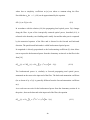
Fig. 4.1 The position of the optical impulse in the fiber core at time t………..32.
Fig. 4.2 The simplified block diagram of the OTDR based reflectometer…….34
Fig. 4.3 Optical Backscatter Reflectometry gives the user unprecedented
visibility into optical components, assemblies, and short-haul
networks………………………………………………………………………..37
Fig. 4.4 Software feature……………………………………………………….39
Fig. 4.5 Sample Time Domain Data From the OBR…………………………...41
Fig 4.6 Return loss in the frequency domain ( bottom plot ) based on
highlighted Section of data in the time domain (top plot)……………………...43
Fig. 5.1 Experimental setup used to perform the experiment………….……….44
Fig. 5.2 Fiber Jumper…………………………………………………………..47
vii
Fig. 5.3 OBR 4200 Luna……………………………………………………….48
Fig. 5.4 Setting menu for the OBR…………………………………………….48
Fig. 5.5 OBR display…………………………………………………………..49
Fig. 5.6 Fiber Jumper………………………………………………………….50
Fig. 5.7 Bending fiber…………………………………………………………51
Fig. 5.8 Bending loss graph display…………………………………………...51
Fig. 5.9 Sleeve splice………………………………………………………….52
Fig. 5.10- 23 meters Jumper…………………………………………………..53
Fig. 5.11 OBR connections…………………………………………………...53
Fig. 5.12 OBR display for a splice……………………………………………54
viii
Abstract
Application on Optical Backscattering Reflectometer (OBR)
By
Hadil Elzein
Master of Science in Electrical Engineering
The main objective of this project is to understand the basics information on bending loss
and splice loss with detail experiment on Luna instrument for a short network fiber. A
historical perspective on fiber optics, fiber types, and application on fiber optics is given.
An emphasis on the theoretical description for Optical Time Domain Reflectometer
(OTDR) and application of the Optical Backscatter Reflectometer (OBR 4200) Luna
instrument are also discussed. A demonstration of the experiment were performed on
Luna Instrument 4200 series OBR by measuring length of a short network fiber, finding
bending loss and using a splice in the experiment. The experiment has been done in
Optiphase Lab, INC.
ix
Chapter 1
Introduction
The technology and applications of optical fibers have progressed very rapidly in recent
years. Optical fiber, being a physical medium, is subjected to perturbation of one kind or
the other at all times. It therefore experiences geometrical (size, shape) and optical
(refractive index, mode conversion) changes to a larger or lesser extent depending upon
the nature and the magnitude of the perturbation. Fiber optics systems have allowed
scientists to make many important advances in the telecommunication, mechanical and
medical fields. Sound, video, and computer communications are more reliable than in the
past. Engineers are able to monitor and maintain safer modes of transportation. And
doctors can perform less dramatic life-improving procedures. The world of fiber optics
has opened many possibilities for solving technological problems and has improved
human civilization.
The business of optical fiber measuring instruments is flourishing: new instruments
offering better performance and facilities are being developed all the time. Such
as(OTDR) Optical Time Domain Reflectometer and (OBR) Optical Backscattering
Reflectometer instruments. Chapter Two of this report gives a historical perspective on
fiber optics, types and applications of optical fiber. Chapter three of this report covers
bending losses and splices losses. Chapter four discusses back scattering Reflectometer
and the newest instruments that are being used in the market.
1
Chapter five demonstrates an experiment using OBR 4200 Luna to find out the length of
a short network fiber, finding bending loss as well as using a splice in the experiment.
this experiment has been done by me in LAB of Optiphase, INC.
2
Chapter 2
Historical Perspective on Fiber Optics
Fiber optic technology is simply the use of light to transmit data. The general use of fiber
Optics did not begin until the 1970s. Since that time the use of fiber optics has increased
dramatically. [1]. The idea of using glass fiber to carry an optical communications signal
originated with Alexander Graham Bell. However this idea had to wait some 80 years for
better glasses and low-cost electronics for it to become useful in practical situations.
The real change came in the 1980s. During this decade optical communication in public
communication networks developed from the status of a curiosity into being the dominant
technology. Among the tens of thousands of developments and inventions that have
contributed to this progress four stand out as milestones:

The invention of the LASER (in the late 1950's)

The development of low loss optical fiber (1970's)

The invention of the optical fiber amplifier (1980's)

The invention of the in-fiber Bragg grating (1990's)
The continuing development of semiconductor technology is quite fundamental but of
course not specifically optical.[2]
2.1 Basics on Fiber Optics
Optical fibers are the actual media that guides the light. They can be made of glass or
plastic. The plastic fibers exhibit much loss and tend to have low bandwidths so glass
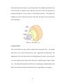
fibers are usually preferred. Figure 2.1 shows A typical fiber that made up of a core,
cladding and a jacket, the core is the center or the actual fiber where the light propagates.
3
It has dimensions on the order of 5 to 600 micrometer. The cladding surrounds the core
and has an index of refraction lower than that of the core, in this way the light will
propagate through the core by means of total internal reflection.
Surrounding the
cladding is the jacket, the outer most part of the fiber. The jacket serves to protect the
entire optical fiber.
Figure 2.1: fiber optic. [3]
2.2 Types of Fiber
There are basically two types of fibers: stepped index and graded index. The stepped
index fibers can be broken down into two types: single-mode and multi-mode. The
stepped index fibers are fibers that have an abrupt change in refractive index from the
core to the cladding while graded index fibers have a gradual change in index (Figure
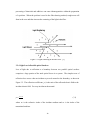
2.2). The multi-mode stepped index fiber has, as one might guess, multiple paths for the
light to travel while the single mode fiber only allows a single light ray to propagate.
4
Because the core diameter is so small, injection laser diode (ILDs) are usually used to
couple light to the fiber. Multimode stepped index fibers exhibit what is referred to as
modal dispersion. This is because not all the rays travel through the center of the core.
Some deviate from the core and are reflected back to the center.
Figure 2.2 Fiber types. [3]
This reflected light takes a longer path and will therefore arrive at its destination at a later
time. The graded index fibers will exhibit less of this dispersion because they gradually
bend light back to the center allowing the light to travel faster when further from the core,
making up for the longer distance. The single-mode stepped index fibers do not exhibit
5
modal dispersion because of their small diameter core. Because of this they tend to have
much wider bandwidths and lower losses.
In general, if the modal dispersion of a fiber is low, then the output signal will be more
likely to resemble the input signal. On the other hand, if the fiber has a high modal
dispersion, the output signal will actually be spread out due to the different path lengths
and therefore will be less likely to resemble the input signal. When such a case is present,
repeaters are needed to re-construct the signal and then send it on its way again. It is
important to consider the characteristics involved when coupling a source to a fiber.
Fibers have a certain ability to collect light. This light gathering ability of the fiber is
called the numerical aperture (NA). A large NA means a larger signal, or ray loss, and
larger distortion “of the intelligence being thus conveyed” [4]. Also with an increase in
NA comes a decrease in bandwidth. The NA is always less than 1 since it is a function of
the refractive indexes of the fiber. There are four parameters that effect the efficiency of
source-fiber coupling, the NAs of both the source and the fiber and the transmissions of
the source and the fiber core [4].
The NA can be represented by the following equations: [2.1] and [2.2]
√
(2.1)
(2.2)
Where
is the index of the core and
is the index of the cladding.
is the half-angle
of the acceptance cone of the fiber. Equation (2.1) is generally used for step-index fibers
while Equation (2.2) is use for graded index fibers.
6
If one were given the indices of the core and cladding of a step index fiber and wanted to
determine its numerical aperture the equation would break down to:
√
(2.3)
Another important fiber parameter is transmission or power loss. Signals that travel
through fibers are sometimes attenuated. This is due to a variety of things such as
impurities in the fiber, scattering within the fiber (variation in the uniformity of the fiber)
and micro bending [4], in which radiation escapes because of small sharp bends that may
occur in the fiber.
(2.4)
Equation (2.4) represents the transmitted power through the fiber [1]. Where
power into the fiber, L is the length of the fiber and
is the
is the attenuation constant
commonly referred to as fiber loss. Typical fiber loss is measured in units of decibels per
kilometer (dB/km) using the relation:
(2.5)
Where
is the loss in decibels. [4]
Fiber loss is a function of frequency so this means that fibers will have greater losses at
some frequencies than others. These losses are usually specified at certain wavelengths
rather than at certain frequencies. Another source of signal loss is at various locations
7
where the light needs to re-enter or exit a fiber. These locations would include coupling
to the fiber (the source end), splicing two fibers together and at the detector end of the
fiber link. In order to minimize losses at these junctions, great care must be taken with the
fiber. Two of the most common forms of splicing are mechanical and fusion splicing, (A
detailed analysis of splice losses will be covered in chapter three) where the fibers are
actually fused together.
The mechanical splice would consist of a connector matting the two ends of the fiber.
Typical real world connectors cause 1 dB of loss each [4]. These losses and other
characteristics of the fiber can be measured with instruments such as an Optical Power
Meter or an Optical Time-Domain Reflectometer (OTDR) or optical Backscattering
Reflectometer (OBR) that will be covered in chapter four. Bending loss is classified
according to the bend radius of curvature: microbend loss or macrobend loss ( A detailed
analysis of bending losses will be covered in chapter three ).
2.3 Application on Fiber Optics
Today fiber optics is used in a variety of applications from the medical environment to
the broadcasting industry. It is used to transmit voice, television, images and data signals
through small flexible threads of glass or plastic. These fiber optic cables far exceed the
information capacity of coaxial cable or twisted wire pairs. They are also smaller and
lighter in weight than conventional copper systems and are immune to electromagnetic
interference and crosstalk. To date, fiber optics has found its greatest application in the
telephone industry [5].
8
Fiber optics is also used to link computers in local area networks (LAN). It is quite
apparent that fiber optics is, at the moment, an invaluable resource but the technology
does have its limitations.
Fiber optics has extended its applications to sensors as well. The advantages of fiber
optic sensors (FOS) in contrast to conventional electrical ones make them popular in
different applications and now a day they consider as a key component in improving
industrial processes, quality control systems, medical diagnostics, and preventing and
controlling general process abnormalities.
Fiber optic sensors have been subject to considerable research for the past 30 years for so
since they were first demonstrated about 40 years ago [2].
These new sensing
technologies have formed an entirely new generation of sensors offering many important
measurement opportunities and great potential for diverse applications. The most
highlighted application fields of FOS are in large composite and concrete structures, the
electrical power industry, Medicine, Chemical sensing, and The gas and oil industry.
9
Chapter 3
Bending Loss and Splice
This chapter introduces the basic information on fiber optic attenuation, and how any
bending in fiber generates loss. Also in this chapter splice losses are being discussed.
3.1 Introduction
Attenuation is the loss of power in a fiber-optic cable or any optical material, and can
result from many causes. During transit, light pulses lose some of their energy. Light
losses occur when the fiber-optic cable are subjected to any type of stress, temperature
change, or other environmental effects. The most important source of lose is the bending
that occurs in the fiber-optic cable during installation or in the manufacturing process.
3.2 Light Losses in an Optical Material
When light passes through an optical component, power is lost in any optical component
is dependent on the accumulative losses due to internal and external losses. Internal
losses are caused by light reflection, refraction absorption, dispersion, and scattering.
External losses are caused by bending, stresses, temperature changes, and overall system
losses. Losses due to refraction and reflection (such as Fresnel reflection, microscopic
reflection, surface reflection, and back reflection) are generally explained by the laws of
light. Common losses due to absorption, dispersion, and scattering mechanisms, as well
as light losses in parallel optical surfaces, and in epoxy that occur in any optical material
are explained below. [6]
10
3.2.1 Absorption
Every optical material absorbs some of the light energy. The amount of absorption
depends on the wavelength of the light and on optical material. Absorption loss depends
on the physical characteristic of the optical, such as transitivity and index of refraction.
The wavelength of the light passing through an optical material is a function of the index
of refracting of the material.
3.2.2 Dispersion
Dispersion is caused by the expansion of light pulses as they travel through optical
components. This occurs because the speed of light through the optical medium is
dependent on the wavelength, the propagation mode, and the optical properties of the
materials along the light path.
3.2.3 Scattering
Scattering losses occur in all optical materials. Atoms and other particles inevitably
scatter some of the light that hits them. Rayleigh scattering is named after the British
physicist Lord Rayleigh (1842-1919), who stated that such scattered light, is not absorbed
by the particles, but simply redirected. [6]. Light scattering in the core of the fiber-optic
cable is a common example, as illustrated in Figure 3.1. The further the light travels
through material the more likely scattering is to occur. Rayleigh scattering depends on
the type of the material and the size of the particles relative to the wavelength of the light.
The amount of scattering increases quite rapidly as the wavelength decreases. scattering
loss also occurs in optical material inhomogeneities introduced during glass reparation
and the additional of dopants in the manufacturing process.
11
Imperfect mixing and
processing of chemicals and additives can cause inhomogeneities within the preparation
of a preform. When the preform is used in the fiber-drawing method, rough areas will
form in the core and thus increase the scattering of the light in the fiber.
Figure 3.1 Light scattering in the fiber core. [3]
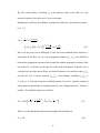
3.2.4 Light Loss in Parallel optical Surfaces
Loss of light due to reflection at a boundary between two parallel optical surfaces
comprises a large portion of the total optical losses in a system. The simplest case of
reflection loss occurs when an incident ray travels normal to the boundary, as shown in
Figure 3.2. The reflection coefficient (
) is the ratio of the reflected electric field to the
incident electric field. For a ray incident at the normal:
(3.1)
where
is the refractive index of the incident medium and
transmitted medium.
12
is the index of the
If
>
, then the reflection coefficient becomes negative. This indicates a 180 phase
shift between the incident and reflected electric fields. The reflectance (R) is the ratio of
the reflected ray intensity to the incident ray intensity. Because the intensity in an optical
beam is proportional to the square of the beam’s electric field, the reflectance is equal to
the square of the reflection coefficient ( ).
The reflectance is calculated as:
[
]
(3.2)
Incident light beam
⇚⇚⇚⇚
Reflected light beam
Transmitted light beam
Figure 3.2 Light beam passing through media. [6]
3.2.5 Light Loss in an Epoxy Layer
Adhesives are used in manufacturing optical devices and are a key technology in the
fiber-optic communications market. In order to produce low-cost and highly reliable
optical components and devices, as easy-to-use, adhesive is necessary. Requirements for
optical adhesive are extremely dependent upon the specific applications. These adhesives
and resins are designed for a specific refractive index. They have high transmittance,
precise curing time, heat-resistance, high elasticity, and permeability. [6]
13
Epoxy adhesives come in several forms. The most commonly used types are one-part,
two-part, and UV-curable systems. One –part systems typically require heat to cure
adhesive. Refrigeration of the liquid adhesive typically prolongs its shelf life. Two-part
systems are based on a chemical reaction and thus must be used immediately after
mixing. Setting times range from several minutes to several hours. UV-light source.
As such, UV-systems do not require refrigeration. These can also be heat-treated to
stabilize the cure.
3.2.6 Attenuation Calculations
Any incident light power passing through an optical component-such as glass microscope
slide, fiber-optic cable, and epoxy layer-is subjected to losses. Attenuation measures the
reduction in light signal strength by comparing output power with input power.
Measurements are made in Decibels (dB). The decibel is an important unit of measure in
fiber-optic components, devices, and systems loss calculations. [6].
(
)
(
)
(3.3)
Equation (3.3) is also used to calculate the loss between the input and output of the cable.
3.2.7 Bending and Micro-Bending
Any bending in a fiber-optic cable generates loss. Fiber-optic cable losses are caused by
a variety of outside influences. These influences can change the physical characteristics
of the cable and affect how the cable guides the light. Certain modes are affected and
losses are accumulated over long distance. However, significant losses can arise from any
14
kind of bending in a fiber cable. The cause of bending loss is easier to envisage using the
ray model of light in a multimode fiber cable. When the fiber cable is straight, the ray
falls within the confinement angle (
) of the fiber cable. However as shown in figure
3.3, a bend will change the angle at which the ray hits the core-cladding interface. If the
bend is sharp enough, the ray strikes the interface at an angle outside of the confinement
angle, and the ray is refracted into the cladding and then to outside as loss. [6]
These are referred as leaky modes, whereby the ray leaks out and the attenuation is
increased.
In another class mode, called radiation mode, power from these modes
radiates into the cladding and increases the attenuation.
In radiation mode, the
electromagnetic energy is distributed in the core and the cladding; however, the cladding
carries no light.
When light is launched into a fiber cable, the power distribution varies as light propagates
down the fiber cable. The power distribution decreases over long distance and eventually
stabilizes. This characteristic of optical fiber is referred to as stable mode distribution.
Stable mode distribution can be observed in a short fiber cables by introducing modefiltering devices.
Mode filtering may be accomplished through the use of mode
scrambling, which can be achieved by bending the fiber cable to form a corrugated path.
The corrugated path introduces a coupling, which leads to existence of both radiation and
leaky modes. Section in chapter five experiments will show a demonstration on bending
loss fiber in a short circuit.
In high-power applications, stable mode distribution can be achieved because the
effective portion of the signal that “leaks” is small in comparison to the full signal
strength.
Mode scrambling allows repeatable laboratory measurements of signal
15
attenuation in fiber cables. Figure 3.3 shows bend in a fiber-optical cable. Micro-bends
can be a significant source of loss. When the fiber cable is installed and pressed onto an
irregular surface, tiny bends can be created in the fiber cable. Light is lost due to these
irregularities.
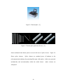
Figure 3.3 Micro-bends and Macro-bends losses. [3]
For a single-mode fiber (SMF) with length( ), bending loss (L) is usually obtained by [7]
(
Where
(
))
(3.4)
is the bending loss coefficient, and it is a function of bending radius,
wavelength of light used in the fiber, and also optical fiber structure and material of the
fiber. Often when bending reaches a critical radius of curvature (
bending cannot be neglected.
(
), then loss due to
is defined as [2]
(3.5)
)
16
is the critical radius of bending,
numerical aperture of the fiber and
is the refractive index of the clad, NA is the
is the wavelength.
Bending loss coefficient (2 ) (dB/km), as proposed by Marcuse, is presented in equation
(3.6). [7]
(
√
)
{ [(
-∑
(
)] }
(
)
Here 2α is the power loss in dB/length,
isthe radius of the fiber core,
(
)
)
(3.6)
is the first order modified Bessel functions,
is the propagation constant,
is the difference
between the propagation constant of the straight fiber and the propagation constant of the
loss modes,
is referred to as the spot size of the mode-field pattern. Equation (3.6) is
)
considered in step index optical fibers, uses Bessel function of zero and first order (
), with boundary conditions
and also the root of Bessel function (
(
)
(
)
. Tsao and Cheng have modified equation (3.6) for 2 , and they considered
other parameters like number of wrapping turns (N), curve fitting function (F), and also V
number. The modified equation is as follows:
[ √
(
)
∑
(
)
]
(3.7)
Where
(3.8)
17
Where R is the radius of curvature of the bend, and for loss they used the following
equation:
(
Where
)
(3.9)
are fitting parameters. Linear relationship between losses and number of
turns is given by:
(3.10)
Where
is the loss due to the number of wrapping turns (N). This sort of simple
equation (linear) is good and valid only for larger radius of curvature, since usually for
higher number of wrapping turns, saturation behavior for bending loss against (N)
happens when radius of the bend is low. In most of these models one can see the effect
of refractive index of the fiber (core and clad) and their differences ( ), which are
important physical parameters. Since guided mode in the fiber core can be transferred to
radiation mode in the fiber cladding induced by bending, it is complicated by the
explanation of simple electromagnetic effects.
3.3 Splicing
The interconnection of optical components is a vital part of an optical system, having a
major effect on performance. Interconnection between two fiber-optic cables is achieved
by either connectors or splices which link the ends of the fiber cables optically and
mechanically. Connectors are devices used to connect a fiber device, such as a detector,
18
optical amplifier, optical light power meter, or link to another fiber cable. They are
designed to be easily and reliably connected and disconnected. The connectors create an
intimate contact between the mated halves to minimize the power loss across the
junction. They are appropriate for indoor applications. Splices are used permanently
connect one fiber-optic cable to another. Splices are suitable for outdoor and indoor
applications. Some types of splices are used to temporarily connect for quick testing
purpose. This chapter covers the operating principles of the splices and describes their
types, properties and operations.
Splices make optical and mechanical connections between two fiber cables. There are
many applications for fiber and splices in fiber systems, such as:

connecting between a pair of fiber cables, using a splice, is an essential part of
any fiber system

Interfacing devices to local area networks.

Splicing may be required on short fiber cables for wiring, testing devices,
connecting instruments and devices, and at other intermediate points between
transmitters and receivers.
3.4 Requirements of Splices
It is very difficult to design splice that meet all the requirements. The lowest losses are
desirable, but the other factors clearly influence the selection of the splice. The following
is a list of the most desirable features for fiber splices required by customers and industry.
19

Low loss (insertion and return). The splice cause low loss of optical power across
the function between a pair of fiber cables.

Easy installation and use.
The splice should be easily and rapidly installed
without the need for special tools or extensive training.

Economical. The splice and special application tooling should be inexpensive.

Compatibility with the environment. The splice should be water proof and not
affected by temperature variation.

Mechanical properties. The splice should have high mechanical strength and
durability to withstand the application and tension forces.

Long life. The splice should be built with material that has a long life in various
applications.
3.5 Fiber Splicing
The splicing process joins fiber-optic cable ends permanently. In general, a splice has a
power loss than a connector. Splices are typically used to join lengths of cable for
outside applications. Splices may be incorporated into lengths of fiber-optic cable or
housed in indoor/outdoor splices boxes, whereas connectors are typically found in patch
panels or attached to equipment at fiber cable interfaces. There are two types of splices:
mechanical and fusion. [6]
3.5.1 Mechanical Splicing
Mechanical splices join two fiber cable end together both optically and mechanically by
clamping them within a common structure. In general, mechanical splicing requires less
20
expensive equipment; however, higher consumable costs are experienced. Figure 3.4
show the sleeves splice.
Figure 3.4 Sleeves splice. [3]
Figure 3.5 shows key-lock mechanical fiber-optic splice, commonly used to quickly mate
and unmate fiber optic cables. It is made from a U-shaped metal part covered by a
transparent plastic body with the two holes on each end. The prepared ends of the fiber
cables are made longer than half of the length of metal power.
Figure 3.5 Key-lock mechanical fiber-optic splice. [3]
The fiber cable is inserted in center hole. When the key is inserted in the second whole
towards the edge of the splice and turned by 90 , the metal part opens and one fiber cable
21
end can be inserted. This operation can be repeated on the other side to insert the second
fiber cable. This type of splice provides a quick and easy way of joining two fiber cables
with low signal loss. It may be used to temporarily or permanently connect fiber cables,
wavelength division multiplexing components, and other fiber-optic elements. [5]
3.5.2 Fusion Splices
Fusion splices is performed by placing the tips of the two fiber cables together by heating
them by fast electrical fusion process so that they melt into one piece. Fusion splices
automatically align the two fiber cable and apply a spark across the tips to fuse them.
They also include instrumentation to test the splice quality and display optical parameters
pertaining to the join. A fusion splice is shown in Figure 3.6. When the fusion splice is
completed, a cylindrical fusion protector is placed over the splice location. Fiber fusion
protectors are made from metal or polymer, and they are applied to insure mechanical
strength and environmental protection. Some types of fusion splice protectors (sleeves)
as sown in figure 3.7 are designed for use in place of the heat shrink method for fast,
easy, and reliable permanent installation. Part of the experiment will demonstrate fiber
splice and the fusion splice protector (sleeves) in chapter five. Fusion splices provide
lower loss that mechanical splices. [6]
22
Figure 3.6 Fusion splice. [3]
Figure 3.7 Fusion splice protector (sleeves). [3]
Some mechanical and fusion splices are used with one of splice closure. Figure 3.8
Shows splice closures.
Splice closures are standard pieces of hardware in the
telecommunication industry for protecting fiber-optic cable splices. Splices are protected
mechanically and environmentally within the sealed closure.
waterproof.
23
Splice closures are
Figure 3.8 Splice closure. [3]
Water is kept out by using non-flowing gel under permanent compression. They are
suitable for indoor, outdoor, and underground cable system installations. There are small
and large closures available for different applications.
3.6 Splice Loss
The most common misalignment at a joint between two similar fibers is the transverse
misalignment similar to that shown in Figure 3.9. Corresponding to a transverse
misalignment of u,( where w is referred to as the spot size of the mode-field pattern) the
power loss in decibels is given by
(
)
( )
(3.11)
Thus a larger value of w will lead to a greater tolerance to transverse misalignment. For
≈ 5 μm, and a transverse offset of 1 μm, the loss at the joint will be approximately
0.18 dB. On the other hand, for
≈ 3 μm, a transverse offset of 1 μm will result in a
loss of about 0.5 dB.
24
Figure 3.9 Splice misalignment. [3]
An Optical Time Domain Reflectometer (OTDR) can be used for splice loss
measurement. A cable section-containing splices are normally shown as knees on the
optical power loss OTDR graph. Splice loss measurements with an OTDR must be
conducted from both directions and averaged (by adding with signs) for accurate splice
loss. It is important to remember that actual splice-loss is the measured splice-loss in both
directions divided with two.
Example:
Splice Loss = [Splice loss A to B + Splice loss B to A] / 2
Splice loss dependent on how accurately the fiber ends are aligned during splicing and
Mode Field Diameter (MFD) of the two fibers. More splice loss can be observed for
misalignment of the fibers and higher difference in MFD values. The MFD is a
characteristic, which describes the mode field (cross-sectional area of light) traveling
down a fiber at a given wavelength. When fibers with different MFD values are spliced
together, a MFD mismatch occurs at splice point. With the help of the following formula
splice loss due to MFD mismatch can be calculated from MFDs (in μm) of two fibers.
Splice Loss (in dB) = 20 Log 1/2 [(MFD1/MFD2 ) + (MFD2/MFD1)]
25
As an application for bending losses and splice losses, The OBR 4200 instrument (newer
version of OTDR) can measure fiber length, bending loss and splice loss in an accurate
way, OTDR theory and BR4200 instrument will be covered in chapter four.
26
Chapter 4
OTDR and OBR
This chapter gives an emphasis on the theoretical description for Optical Time Domain
Reflectometer (OTDR) and discusses the applications of the Optical Backscatter
Reflectometer (OBR4200) Luna instrument.
4.1 Basic principles of the backscattering method
The backscattering method was invented by M. Barnoskim and M. Jensen in 1976 [8], in
time when technology of the optical fiber manufacturing was at early stages. The precise
and reliable measurement of local losses on the fiber was very important for further
improvement of quality of fibers. The basic idea of the proposed method consisted in
launching a rather short and high power optical impulse into the tested fiber and a
consequent detection of back scattered optical power as a response of the fiber to the test
impulse. The detected signal provides the detail picture about the local loss distribution or
reflections along the fiber caused by any of the attenuation mechanisms or some other
non-homogeneities on the fiber. An important feature of the method is non-destructivity
and the fact that the access to only input end of the fiber is needed.
The measurement of the time delay of the detected signal from the fiber end or from any
perturbation on the fiber allows to derive the information about the perturbation
localization provided that the index of refraction in the fiber core or group velocity of
light propagation is known. In any point on the fiber the magnitude of the backscattered
optical power is proportional to the local transmitted optical power. Due to the nonzero
losses this power is gradually attenuated along the fiber and consequently also the
27
backscattered power is also attenuated. The measurement of the backscattered power as a
function of time or position on the fiber gives the information about the local distribution
of the attenuation coefficient along the fiber. In this way one can evaluate the space
distribution and magnitude of various non-homogeneities along the fiber like optical
connectors, splicing, micro- and macro-bend losses and others measurand-perturbances.
The comparison of the losses closely before and after point of interest makes possible to
evaluate insertion losses of the various optical components on the fiber link.
4.1.1 Theoretical description of the OTDR
The elementary experimental experience gives the relation describing the dependence of
the optical power propagating along the optical fiber as a function of the distance x
( )
( )
(4.1)
Where ( ) is the total optical power at the distance x from the point of launching the
input optical impulse,
is the value of the input optical power (x = 0), α is the total
attenuation coefficient and 1(x) is the Heaviside step function. In practice the attenuation
coefficient is usually expressed in dB/km. In this case the relation (4.1) can be rewritten
into the form
( )
( )
(4.2)
Where
is the total attenuation coefficient given in units dB/km. The mutual equation
between
and
is defined by
(4.3)
28
Total losses in the fiber are caused by different mechanisms and the total attenuation
coefficient can be different at any point on the fiber. As a result it is necessary to rewrite
the equation (4.1) into more general form. [9]
∫
( )
( )
( )
(4.4)
Where the local attenuation coefficient α(x) is now a function of the distance x. It be
shown that the total attenuation coefficient can be roughly split into two components
( )
( )
( )
(4.5)
( ) represents the absorption losses and
Where
( ) represents the losses by
Rayleigh scattering mechanism. The average value of the total attenuation coefficient
(x) on the fiber section defined by distance (0, x) can be calculated according to the
equation [9]
∫
( )
(4.6)
The equation (4.4) can be simplified as follows
( )
( )
The elementary optical power
(4.7)
scattered by the Rayleigh mechanism on each
elementary fiber section dx (scattering center) at the distance x from the input end of the
fiber is given by
( )
( )
( )
(4.8)
29
( ) was taken as constant along the fiber.
where due to simplicity coefficient
Provided that
( )
<< 1, (4.8) can be approximated by the equation
( )
(4.9)
In accordance with the relation (4.4) the propagating local optical power P(x) changes
along the fiber. A part of the isotropically scattered optical power, described (4.9), is
refracted at the boundary core/cladding and is totally lost and the other part is recaptured
by the numerical aperture of the fiber and is directed in the forward and backward
direction. The part directed backwards is called backscattered optical power.
Its magnitude is directly proportional to the backscattering coefficient (S) what allows
one to express the backscattered power from the elementary section
on the fiber in the
form [10]
( )
( )
[
( )
∫
]
( )
(4.10)
The backscattered power is, similarly as forward propagating total optical power,
attenuated on the route to the input end of the fiber. The backward attenuation coefficient
(let us denote it by α''(x)) is generally different from the forward attenuation coefficient
(x).
As a result one can write for the backscattered power from the elementary section dx in
the point x, that can be detected at the input end of the fiber, the equation
( )
[
∫ [ ( )
( )]
]
( )
30
(4.11)
If one takes
and
as the total average attenuation coefficients at the distance x in
forward and backward direction respectively and A will represent their arithmetical
average A = 0.5(
), then the equation (4.11) can be transformed into the form
( )
( )
(4.13)
For the backscattering coefficient S one can derive the analytical relation describing its
magnitude for the single-mode and multi-mode fibers with a given refraction index
profile. Under some simplifications a rather simple equation for the backscattering
coefficient for a single-mode optical fiber can be obtained in the form. [9]
(
(
)
(4.14)
)
For the case of a multi-mode fiber with a step-index profile the backscattering coefficient
can be described by
(
)
(
)
(4.15)
(4.16)
where NA = ( (n12 - n22)1/2 is the numerical aperture,
the core and cladding respectively,
,
are the refractive indexes of
is the mode field diameter of the basic mode,
is
the fiber core radius, V is so called normalized frequency V = (2πa/λ)NA.
The time dependence of the backscattered power detected at the input end of the fiber as
a response to the testing impulse of the optical power. For this purpose let us consider the
optical fiber into which an optical impulse of the instantaneous power P0 and the width T0
31
was coupled in the time t = 0. The time dependence of this impulse is given by the
equation
( )
[ ( )
(
)]
(4.17)
Where 1(t) is the Heaviside unit step function. One can imagine this impulse as a lit
section of the fiber. The length of the region is given by Δx = vgT0, where vg is the group
velocity of the impulse propagation in the fiber. The position of the trailing edge of the
impulse at time (t - T0) is given by x and the position of the leading edge is given by
(x + Δx). The described situation is outlined in the Figure 4.1.
Figure 4.1 The position of the optical impulse in the fiber core at time t. [9]
Using the substitution
, resp.
, the equation (4.13) can be rewritten
into the form
( )
(4.18)
32
The time dependence of the backscatter power generated by the whole testing impulse
can be obtained by the integration
( )
∫
(4.19)
Provided that AvgT0 << 1, which is for high quality fibers. Equation (4.19) can be
transformed into the form
( )
( )
(4.20)
Using the same substitution as it was done for the equation (4.18) the time dependence of
the backscattered power can be described by
( )
( )
(4.21)
In the case of high quality fiber the attenuation coefficient α is given by α = A. It makes
possible to write for the backscattered power the well-known equation
( )
( )
(4.22)
If the fiber parameters (S, αrs, α, vg) are constant and the maximum launched power is P0,
then the maximum detectable backscattered power can be enhanced by the increase of P0
and T0, which define the energy of the impulse.
33
4.1.2 The main aspects of the signal processing in OTDR
A simplified block diagram of the OTDR-based optical reflectometer is given in the
Figure 4.2. The main blocks of the reflectometer are the generator of the testing impulse
and the detection system of the backscattered light. The remaining blocks provide the
suitable timing of signals (clock generator) and the interpretation of the measured data
(display). A 3-dB fiber power splitter makes possible to couple the optical excitation
power impulse into the tested fiber and simultaneously to deviate the backscattered power
to the optical receiver. [10]
Figure 4.2. The simplified block diagram of the OTDR based reflectometer. [10]
The crucial element of the device is the block for the processing of the signal from the
optical receiver. For the signal recovery a technique of signal sampling using the A/D
converter simultaneously with the signal averaging method is used. For the elimination of
the dead zone a blind subsidiary fiber put between the optical source and the input end of
34
the tested fiber is used. In this way the Fresnel reflection from the input end of the tested
fiber and subsequent dead zone occurs in the time corresponding to the section of
subsidiary fiber and no information coming from the tested fiber is lost due to dead zone.
35
4.2 Overview (OBR 4200 Luna)
Luna Technologies’ Optical Backscatter Reflectometer (OBR) is the industry’s first ultrahigh resolution OTDR with backscatter- level sensitivity designed for component- and
module-level reflectometry. The OBR uses swept-wavelength coherent interferometry to
measure minute reflections (< 0.0003 parts per billion) in an optical system as a function
of length with spatial resolution down to 10 μm. This provides the user with
unprecedented optical inspection and diagnostic capabilities. The OBR can be used to
locate and troubleshoot splices, connectors, fiber bends and breaks, fiber segments, and
components embedded in a short run fiber assembly. With integrated temperature and
strain sensing, the OBR gives you the ultimate in fiber diagnostics. [11]
4.2.1 Measurement Performance
• -125 dB sensitivity
• 70 dB dynamic range
• Up to 500 meter length range
• 10 μm spatial resolution
• 0.05 dB loss resolution at -100 dB reflectivity
4.2.2 Application
• System design verification and analysis that can discriminate between individual
devices, connectors, fibers, splices and components.
36
• Component qualification for inspection and rapid testing of individual optical
components.
• Troubleshooting of optical systems during development and production.
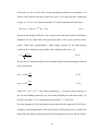
• Failure analysis of devices and subassemblies.
• Distributed sensing capabilities – temperature and strain.
4.2.3Backscatter vs. Conventional Reflectometer
Figure 4.3. Optical Backscatter Reflectometry gives the user unprecedented visibility into
optical components, assemblies, and short-haul networks. [11]
37
Reflectometry is based on propagating a test signal through an optical system or network
and monitoring the reflected portion of that signal to get a picture of locations in the
system or network that cause reflections.
Optical time-domain reflectometry (OTDR) uses short optical pulses as probes of the
reflections in a network.
This well-known technique is suited for measuring long
network spans with relatively low resolution (meters) and medium lengths with medium
resolution (centimeters).
Optical Backscatter Reflectometry is based on a frequency-domain technique, optical
frequency-domain reflectometry (OFDR), that uses a tunable laser and an interferometer
to probe reflections. Frequency-domain techniques are usually used to analyze systems
on the component- or module-level when a very high-resolution (microns) analysis of the
reflections in a system is required.
Optical backscatter reflectometry differs from other frequency-domain techniques in that
it is sensitive enough to measure levels of Rayleigh backscatter in standard single-mode
fiber. The figure above illustrates how this can be used to measure both reflective and
non-reflective loss as light propagates down a simple optical system.
Furthermore, Luna’s OBR can be used to measure the distributed spectral shift and
temporal shift in the Rayleigh backscatter along an optical fiber. This capability enables
distributed temperature and strain sensing with any standard telecom-grade fibers (graded
index multimode as well as single mode). This technique enables robust temperature and
strain measurements with high spatial resolution and accuracy. Because the measurement
does not require specialty fiber, the method may be applied to existing fiber paths which
were never intended to act as a sensor. This measurement capability also provides a
38
practical and economical alternative to fiber Bragg gratings and extrinsic Fabry-Perot
interferometric sensors in situations where a large number of closely spaced
measurements are desired.
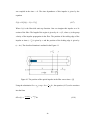
4.2.4 Software Features
The Luna OBR control software includes an intuitive graphical interface. All controls,
options, and measurement results are easily accessible from the single main window or
the menu bar.
Figure 4.4 Software feature. [11]
39
The Luna OBR control software includes an intuitive graphical interface. All controls,
options, and measurement results are easily accessible from the single main window or
the menu bar.
Software features:
• System Control provides wavelength settings and scan control.
• Frequency Data Results contains a control for calculating frequency-domain data and
indicators that display the current wavelength resolution and the average loss of the
device under test.
• Graph Cursors display the graph coordinates for the current cursor settings. The cursors
also allow the user to compare backscatter levels in different portions of the network
and calculate the insertion loss between those two points in the network. The example
above shows an insertion loss of 0.32 dB occurs at about 7 meters down the network
under test.
• Graph Areas display measured data. The top plot is a graph of the time-domain data,
and the bottom plot is a graph of time or frequency-domain data with higher resolution.
Buttons on each graph control how a plot appears in the window, including multiple click
and- drag zoom features as well as manual scaling options.
40
Because the Luna OBR measures the full scalar response of the device under test,
including both amplitude and phase, it is possible to convert back and forth between time
domain and frequency-domain data. The main screen displays time-domain data in the
upper graph, and frequency-domain data in the lower graph. Both amplitude and phase
information can be displayed in either domain. [11]
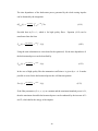
4.2.5 Time Domain
By default, the upper graph displays the amplitude of the time-domain data, which
produces a plot in which each reflection within the network under test produces a peak.
This provides a quick and reliable means for identifying and locating reflections within a
system.
Figure 4.5. Sample Time Domain Data from the OBR. [11]
41
4.2.6 Frequency Domain
The data in the frequency-domain plot is calculated based on the cursor location and
integration width of the time-domain data contained in the plot window above. Therefore
it is possible to sectionalize a device or system and determine the amplitude and phase
response of each interface or optical path separately, by zooming in and isolating them in
the time-domain plot. This provides a powerful means for quickly and easily identifying
faults and pinpointing their cause within a component, module, or subsystem.
The lower plot can display both the amplitude and phase derivative of the frequency
domain data. The amplitude corresponds to the return loss of the device under test. By
selecting a single reflection in the time-domain plot, it possible to measure the return loss
from each interface individually within a device or subassembly. The Integrated Loss
indicator yields a single average loss value for quick pass/fail evaluation for each optical
path or interface.
The phase derivative plot in the frequency-domain yields the group delay of the device
under test. Again, the group delay characteristics of individual optical paths within a
device can be characterized by selecting the appropriate impulse in the time-domain plot.
42
Figure 4.6. Return loss in the frequency domain (bottom plot) based on highlighted
section of data in the time domain (top plot). [11]
43
Chapter 5
Experimental studies using OBR
Chapter five demonstrates experimental studies that were performed on Luna instrument
4200 series OBR. The details are as follows.
5.1 Objective of the Experiment:
To find out the length of a short network fiber, finding bending loss, and to locate a splice
on a fiber. This experiment had been done by me in in LAB of Optiphase, INC.
5.1.1 Equipment:

OBR 4200

Fiber Jumper 253.5m long, single mode fiber 3 m, and 23 m single mode fiber.

Splice
5.1.2 Experimental Setup
Power
Supply
OBR 4200
Fiber Test
Figure 5.1 Experimental setup used to perform the experiment [3]
44
5.1.3 OBR Specification:
The OBR 4200 Luna instrument comes equipped with exhaustive user manual. Due to
the fragility of the OBR equipment, it was that the instructions in the manual were
accurately followed. The manual also held specification for the instrument.
Specifications are as follows.
PARAMETER SPECIFICATION UNITS
Maximum Device Length:
Device length
0 to 500 m
Spatial Resolution:
Event resolution
< 3 mm
Sampling resolution
0.3 mm
Center Wavelength:
1542 nm
Integrated Return Loss Characteristics:
Dynamic range
50 dB
Total range
-10 to -120 dB
Sensitivity
-120 dB
Resolution
±0.2 dB
Accuracy
±0.4 dB
45
Integrated Insertion Loss Characteristics:
Dynamic range
16 dB
Resolution
±0.1 dB
Accuracy
±0.2 dB
Measurement Timing
2.6 seconds overhead per scan plus
0.12 s/m
Optical Output
Connector type
FC/APC -
Output power
10 mW
Launch condition
Single-mode output standard.
Multimode output available with
Mode-Conditioner accessory.
Environmental
Operating temperature
0 to +40 C
Storage temperature
-20 to +60 C
Power
Battery life
5 hr
Battery charging time
5 hr
Dimensions and Weight
Size
8.5(L) x 10.7(W) x 3.85(H) in
Weight
9.8 Ibs
46
5.2 Observation:
5.2.1 Measuring Fiber Length Using OBR4200
In this case a 253.5m fiber jumper (Figure 5.2), this kind of Jumper is used for all kind of
industry and it is a single mode fiber, the jumper has a splice around it. It is connected to
the OBR4200 Luna as shown in (Figure5.3). In the setting menu the length starting
from100m to 300m as shown in (Figure 5.4). We measure basically from the beginning
of it to the back reflection of the end of this jumper. It tells us where the end of the fiber
is, measuring time it takes for wave length 1.5 micro- meter to travel down the jumper hit
the back reflection of 4% of the selected end and comeback.
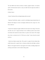
Figure 5.2 Fiber Jumper [12]
47
Figure 5.3 OBR 4200 Luna [12]
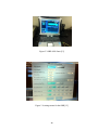
Figure 5.4 settings menu for the OBR [12]
48
When the scan on the OBR4200 is operating, the graph display shows the length of the
fiber jumper (where the red line is X2=253.66m) is 253.66m long, this is a very accurate
measurement ( Figure 5.5).
Figure 5.5 OBR displays [12]
49
5.2.2 Fiber Bending Loss
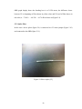
In this case: A three meter fiber jumper (Figure 5.6) is connected to the OBR, this time a
bending fiber was demonstrated(Figure 5.7) in order to find the bending loss location on
the OBR graph display.
Figure 5.6 Fiber jumper [12]
50
Figure 5.7 Bending fiber [12]
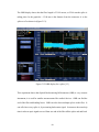
Figure 5.8 Bending loss graph display [12]
51
OBR graph display shows the bending loss is at 3.0330 meter, the difference losses
between X1 is (beginning of fiber-shown in yellow color) and X2 (end of fiber-shown in
red color) is -72.630
- 60.238 = - 6.176 dB as shown in (Figure 5.8).
5.2.3 Splice Fiber
In this case a sleeve splice (figure 5.9) is connected to a 23 meter jumper (Figure 5.10)
and connected to the OBR (figure 5.11).
Figure 5.9 Sleeve splice [12]
52
Figure 5.10 - 23 meter jumper [12]
Figure 5.11 OBR connections [12]
53
The OBR display shows that the fiber length is 23.149 meters, at 2.246 mm the splice is
taking place. In the graph dx = 15.08 mm is the distance from the connector x1 to the
splice at x2 as shown in (figure 5.12).
Figure 5.12 OBR display for a splice [12]
This experiment shows that Optical Backscattering Reflectometer (OBR) is very accurate
instrument, it is used for smaller measurements like medical devices. OBR can find the
end of the fiber and bending losses. OBR can also detect multiple splices in the fiber. It
can tell where every splice is, by measuring backscatter signal. It measures the round trip
time it takes an optic signal to travel from one end of the fiber till the splice end and back.
54
OBR 4200 is the industry’s only portable device. It cost $60,000. OBR does a very fine
measurements and it has an amazing accuracy.
55
References
[1] Joseph C. Palais, “ Fiber Optic Communications”, Prentice-Hall, 1984
[2] H J R Dutton, Understanding optical communications,
http://www.Redbooks.ibm.com 2-14,2012.
[3] Broad band suppliers.,
http:// broadbandsuppliers.com-fiber - optics 3-23, 2012.
[4] Edward A. Lacy, “Fiber Optics”, Prentice-Hall, 1982
[5] Bahareh Gholamzadeh, and Hooman Nabovati, “Fiber optic Sensors”,
World Academy of Science, Engineering and Technology, 2008
[6] Abdul Al-Azzawi, “ Fiber Optics”, Principles and Practices, 2007
[7] D Marcose, Appl. Opt. 23, 4208 (1984)
56
[5] By Rongqing Hui, Maurice S. O'Sullivan - Academic Press (2008) -“Optic
Measurement Techniques”.
[8] By Rongqing Hui, Maurice S. O'Sullivan - Academic Press (2008) -“Optic
Measurement Techniques”.
[9] M. Nazarathy, S. A. Newton, R. P. Giffard, D. S. Moberly, F. Sischka, W. R. Trutna
and S. Foster, "Real-Time Long Range Complementary Correlation Optical Time
Domain Reflectometer", J. Lightwave Tech., 1989
[10] M. Nakazawa, M. Tokuda, K. Washio and Y. Morishige, "Marked Extension of
Diagnosis Length in Optical Time-Domain Reflectometry Using 1.32 μm YAG Laser",
Electron. Lett., vol. 17, 1980
[11] OBR 4200 Instrument, www.lunatechnologies.com 3-25, 2012.
[12] LAB of Optiphase, INC.
57