1
ZOOM User Manual Version 1512 03 December 2015 ZOOM is a product of Trajectory Solution Huntsville, Alabama http://trajectorysolution.com [email protected] NOTE: The Graphical User Interface images in this manual generally do not apply to the same mission. TABLE OF CONTENTS TABLE OF CONTENTS [Page Numbers in Brackets] 1. INTRODUCTION [1] 2. FIRST WINDOW [6] 3. MISSION SELECTION [7] 4. MISSION SYNOPSIS [10] 5. MISSION SUMMARY [15] 6. MISSION DEFINITION: Intercept Spacecraft Or RV 7. MISSION DEFINITION: Inject Into Conic [24] 8. MISSION DEFINITION: Achieve Specified State 9. CENTRAL BODY MODEL [26] [28] 10. EXPONENTIAL ATMOSPHERIC MODEL [30] 11. LAUNCH AND IN-FLIGHT CONDITIONS 12. WIND MODEL [21] [31] [36] 13. AERODYNAMIC HEATING-RATE MODEL 14. ROCKET STAGE STACK [38] [39] 15. CONFIGURE STRAP-ON BOOSTER 16. CONFIGURE TANDEM STAGE [42] [45] 17. AERODYNAMIC FORCE MODELS [56] 18. NORMAL, AXIAL AERODYNAMIC FORCE MODEL 19. LIFT, DRAG AERODYNAMIC FORCE MODEL 20. NORMALIZED THRUST PROFILE 21. STAGE SIZING FACTORS 22. LAUNCH PREPARATION [58] [61] [65] [67] [69] 23. OPTIMIZER PARAMETERS [71] 24. PRECISION AND OUTPUT PARAMETERS [73] 25. RECOMMENDED SOLUTION PROCEDURE 26. SOLUTION WINDOW 27. PLOT SELECTION 28. EFFECTS [74] [77] [79] [85] APPENDIX A: COORDINATE REFERENCE FRAMES [90] APPENDIX B: PARAMETERS FOR SINGLE-ENGINE-EQUIVALENT ROCKET MOTOR [93] i 1. INTRODUCTION 1. INTRODUCTION ======================================== ZOOM is a computer program for the conceptual design and analysis of rockets and their missions in the vicinity of a single "central body" such as the earth. The program incorporates insights and methods that were employed during America's developments of the Saturn V moon rocket and the Space Shuttle. It is important to note that, in some places in this manual, the term "earth" is used where it would have been more appropriate to use the term "central body". You have the flexibility to modify the default gravitational, dimensional, atmospheric, and rotational parameters and so define a central body other than the earth. ZOOM can be operated via its graphical user interface (GUI) with a touch-screen interface as well as with a mouse/keyboard interface. The program has been checked out with Windows XP, Windows 7, and Windows 8.1 operating systems. However, with Windows 8.1 a "program has stopped working" error sometimes occurs, apparently at random times. As far as is known, the Windows 8.1-related error has never been encountered on computers with Windows XP or Windows 7 operating systems. And, constructive results can often be obtained on a computer with the Windows 8.1 operating system before the "stopped working" error is encountered. ZOOM's optimization procedure was created in the early 1970's and enhanced over a subsequent period of 35 years. The procedure uses the Simplex algorithm1 in a novel and powerful way that has found quasi-optimum solutions for a wide variety of trajectoryoptimization problems. The modeled rocket's tandem stages are defined by core ideal delta-velocities, propellant mass fractions, and core thrust-to-weight-ratios. From these quantities, ZOOM calculates the propellant loads, inert masses, and thrusts. The rocket is treated as a point-mass with three degrees of freedom. The rocket is symmetric with respect to its "pitch" plane. The rocket rolls automatically to keep its pitch plane in the plane defined by the rocket's relative velocity and longitudinal axis. The rocket thrusts along its longitudinal axis, so both the thrust and aerodynamic forces remain in the rocket's pitch plane for the duration of the flight. You can opt to specify the thrusts and/or propellant loads of one or more of the rocket's tandem stages, or you can set maximum limits on the quantities. The program treats these specifications as constraint equations or inequalities and satisfies them during its iterative optimization procedure. The thrust and/or burn time of a strap-on booster can be fixed or optimized within maximum limits. If the thrust and burn time are both optimized, they can be optimized independently (within the specified limits), or their optimization can be constrained to keep the strap-on booster's propellant at a specified value. 1 The Simplex algorithm was created by George B. Dantzig, Ph.D. in the 1930's to solve linear programming problems and has proven to be unusually robust and effective in this application. 1 1. INTRODUCTION REFERENCE FRAMES Rocket motion is computed in a central-body-fixed frame with origin at the launch site. The three orthogonal axes of this right-handed frame are pointed north, east, and down (along the plumb line). This frame is termed the "north-east-down" frame, abbreviated NED. For an 'Intercept Satellite or RV' mission, the target motion is computed in an earth-centered inertial frame, abbreviated ECI. Some computations are done in an earth-centered, earthfixed frame, abbreviated ECF. Various output data are also expressed in this frame. The NED, ECI, and ECF frames are defined in Appendix A. GRAPHICAL USER INTERFACE ZOOM's graphical user interface (GUI) facilitates the creation of new missions and the examination of completed missions. Navigation among the GUI's primary sequential windows is done via navigation buttons at the bottoms of the windows. These buttons and their associated destination windows are: Navigation Button [Mission Type] [List] or [ReZOOM] [Synopsis] [Mission] [Conditions] [Stack] [Countdown] Destination Window First window Mission Selection Mission Synopsis Mission Definition Launch and In-Flight Conditions Rocket Stage Stack Launch Preparation The navigation buttons are arranged in a single row at the bottom of the primary sequential windows. The buttons are positioned left-to-right in the usual order for creating a new mission. The recommended procedure for creating a new mission is described in the 'Recommended Solution Procedure' section (Section 24). CONTENTS OF THE ZOOM PROGRAM DIRECTORY All files needed for the operation of ZOOM are in the 'ZOOM Program Directory', which contains the folders: 'Aerodynamic File Library', 'DATA', 'Help', and 'Trash', and the files: 'salflibc.dll' and 'ZOOM.exe' (the program executable file). The default 'salflibc.dll' file is intended for use with Windows operating systems newer than Windows XP. For Windows XP and earlier operating systems, this file should be replaced with the 'salflibc.dll' file in the DLL-XP folder that is included in the 'ZOOM Folder'. The 'Aerodynamic File Library' folder contains any Lift, Drag aerodynamic data files which have been created off-line or which have been named and copied to the folder using the GUI. Normal, Axial aerodynamic data are included in the 'rocket.dat' files in the mission 2 1. INTRODUCTION subfolders. Each mission uses one of the two kinds of aerodynamic models: Normal, Axial (the default linear model) or Lift, Drag (a higher-fidelity model). The 'DATA' folder contains the mission subfolders for all missions that have been defined and solved. The folder also contains two small files: 1) 'bkgrndColors.dat', which defines the two window-background colors that distinguish missions having Metric and English units, and 2) unitsOut_default.dat, which identifies the units (Metric or English) chosen for the last mission solved by the program. The 'Help' folder contains the plain text files that comprise the contextual help information. The content of the appropriate file is displayed by the GUI when an 'INFO' button is clicked. Although it is not encouraged, you may modify these plain text files to make the explanations clearer to you as you gain experience using the program. If you do modify a file, you should use a plain-text application, such as Notepad, and the word-wrap option should be deactivated. Each line of text should be ended by clicking the keyboard's "Enter" or "Return" key. And, the length of each line should be kept within the maximum line length observed in the original file so that the entire line can be seen in the GUI's displayed window. The 'Trash' folder contains the mission subfolders that have been deleted via [Delete] in the 'Mission Selection' window. The 'Trash' folder should be periodically emptied off-line (into the Windows Recycle Bin) using the operating system's file-management application (e.g., Windows Explorer, File Explorer, etc.) MISSION SUBFOLDERS Each mission's data are saved in a subfolder within the 'DATA' folder. The mission-subfolder names begin with a two-letter prefix that identifies the mission type: 'ES' for 'Achieve Specified State' missions, 'OI' for 'Inject into Conic' missions, and 'SI' for 'Intercept Spacecraft or RV' missions. These two letters are followed by a six-digit (yymmdd) missioncreation date, automatically assigned by the program. The six-digit date is followed by a space and then by the mission's core name that you supply. When the 'DATA' folder is opened via the operating system's file-management application, the mission subfolder names look like these examples: ES120824 One Stg Max Speed to Given FPA and Altitude OI120621 Three Stg 100 x 600 Nmi - Thrust Profile for All Stages SI120622 Rendezvous in Sun-Sync Orbit - Min Initial Mass When mission subfolder names are listed in the 'Mission Selection' window, the two-letter prefixes are not shown, and the dates appear as suffixes of the form: ' - 14Apr09'. Each mission's data files are stored in its mission subfolder. You have access via the 'Data Files' button in the 'Mission Synopsis' window to view the essential data in these files. INPUT DATA FILES Each mission, regardless of type, always has the following eight input data files: 'earth.dat' 'mDescrip.dat' parameters of the central body. a user-supplied descriptive narrative. 3 1. INTRODUCTION 'mission.dat' 'rocket.dat' 'wind.dat' 'optimizer.dat' 'precision.dat' 'units.dat' mission definition data (file format of depends on the mission type). rocket definition data. characterization of the wind (if any). optimization control parameters. computational precision control. indicating either 'Metric' or 'English' units. For each stage using the Lift, Drag aerodynamic force model, the mission subfolder also includes a Lift, Drag file with a generic name (e.g., 'LDfile_1.dat','LDfile_2.dat', etc.). OUTPUT DATA FILES Each mission's output data files are contained in an 'output' subfolder within the mission subfolder. All missions have the following twelve output data files: 'summary.dat' essential data describing the solution (format depends on mission type). 'output0.dat' event timeline and other data. 'output1.dat' time histories of rocket-trajectory variables in a central-body-fixed frame. ''output2.dat' primarily time histories of forces, accelerations, propellant remaining, dynamic pressure, and Mach number. 'output3.dat' time histories of gravitational acceleration in both the ECF and NED frames; atmospheric density, pressure, and sound speed; Mach number (redundant); and wind speed. 'output4.dat' primarily time histories of the rocket's position and velocity components in the NED frame and of the acceleration (coriolis and centrifugal) due to the frame's angular velocity, also expressed in the NED frame. 'rocket conic.dat' the epoch, osculating elements, and orbital period of the rocket's conic at burnout. The orbital period in this file is that which would apply if the central body's atmosphere or surface were not encountered. 'rocket states.dat' primarily time histories of the rocket's position and velocity components in the ECF and ECI frames. 'solution.dat' results of ZOOM's optimization procedure, showing initial and final values of the variables being optimized, initial and final values of the scaled objective and constraint functions, scale factors, and history of the iterative procedure. 'effects.dat' list of variables being optimized, effects of perturbations of the variables on the objective and constraint functions, and other factors, all viewable via the GUI. 'variables.dat' control-variable values for each iteration of the optimization procedure. 'delv_losses.dat' time histories of the ideal delta-velocity and delta-velocity losses. 4 1. INTRODUCTION An 'Intercept Spacecraft or RV' mission has at least three additional output files: 'output5.dat' time histories: target position and velocity components in the NED frame; target altitude, geodetic latitude, and longitude; target ground range from launch site. 'target states.dat' time histories of the target's position and velocity in the ECF and ECI frames. 'target drag.dat' time history of the target's post-launch drag deceleration (significant only for missions where the target descends to low altitude). There are sometimes as many as three other files in the output subfolder for an 'Intercept Spacecraft or RV' mission: 'tgtElem.dat' time histories of the target's osculating conic elements prior to the displayed pre-launch ground track. This file is created whenever a plot of the target's pre-launch ground track is activated. 'opportunities.dat' list of possible launch opportunities during launch window, based on target's ground track and the launch point. 'latlong.dat' time histories during launch window of target's latitude, longitude, altitude, and slant range from launch site to target. VIEWING THE DATA FILES Most input and output data files can be viewed in their raw forms via the GUI and copied to the keyboard buffer when a mission is examined via 'Mission Synopsis'. It is normally not necessary to access the files off-line using the operating system's file-management application. If the files are examined off-line, CARE MUST BE TAKEN TO NOT ALTER THEM. And, none of the files should be selected by the operating system's file-management application when the program is being executed. 5 2. FIRST WINDOW 2. FIRST WINDOW (Select Mission Type) =========================== Click the bubble for your chosen mission type: a) Achieve Specified State, b) Inject into Conic c) Intercept Spacecraft or RV A 'Mission Selection' window will be displayed from which you can select an existing mission for a template or start your mission from scratch. Depending on mission type, you will be able to choose one of several objectives - which include maximum payload, minimum initial mass, minimum flight time, maximum range, etc. and you will be able to define your mission constraints. [INFO] buttons appear in many of the GUI windows. These buttons display the text of the relevant section in the User Manual and thus provide contextual help information. Click the [COLORS] button to choose window background colors. You can pick different background colors for missions based on Metric and English units to help distinguish them. The [COLORS] button only appears in this window. Click the [QUIT] button to immediately quit and close the program. This button also appears in several other windows. Click the [Developer's Statement] button for a link to the developer's website and for the developer's email address. Links are also provided for three Children's hospitals, and a suggestion is made for donations to one of these or to a charity of your choice. There is no obligation to donate however. The ZOOM program is available for you to use as you please, free of charge. 6 3. MISSION SELECTION 3. MISSION SELECTION ===================================================== The 'Mission Selection' window is activated when you click one of the missiontype bubbles in ZOOM's "First" window. Clicking the [Mission Type] button returns you to the "First" window. Access to the 'Mission Selection' window from windows other than the "First" window is via the [List] button. The 'Mission Selection' window is the only window from which you can access the "First" window and the 'Mission Synopsis' window. All existing missions of the chosen type that are in the 'Data' folder are listed in this window. A so-called "Mission from Scratch" is included at the top of the list. If you don't want to use an existing mission as a template for a new mission, you can select the "Mission from Scratch". You select a mission from the list by left-clicking it. By default, the missions are listed in inverse chronological order according to their creation dates (most recent first). To get an alphabetical listing you click [Change to Alphabetical List]. The alphabetical ordering is defined by the ASCII sequence, where numerals precede letters and upper-case letters precede lower-case letters. You can return to the inverse chronological listing by clicking the [Change to Chronological List] button which will appear when the alphabetical list is displayed. The displayed names differ from the names of the files in the 'DATA' folder in that the mission-type indicator ('ES', 'OI', or 'SI') has been removed and the six-digit creation date has been moved to the end of the name and reformatted in a day/month/year sequence (e.g., 07Jun14). The name as listed, but excluding the date suffix, is defined as the mission's "core" name. NAVIGATION BUTTONS The row of buttons at the bottom of the 'Mission Selection' window are the "navigation" buttons that you use to navigate back and forth between the program's primary windows. The navigation buttons and their corresponding destination windows are: 7 3. MISSION SELECTION Navigation Button [Mission Type] [List] or [ReZOOM] [Synopsis] [Mission] [Conditions] [Stack] [Countdown] Destination Window "First" Mission Selection Mission Synopsis Mission Definition Launch and In-Flight Conditions Rocket Stage Stack Launch Preparation CHOICE OF UNITS Click the [Toggle Units] button to alternate between Metric and English units for display and data entry. A new mission's data will be saved in the chosen units. When you choose an existing mission as a template, changing the units for your new mission will not affect the original template mission. The 'Mission Selection' and 'Mission Synopsis' windows are the only windows where you can choose/change the units. DELETE SELECTED MISSION You can remove a mission from the mission selection list via the [Delete] button. This action moves the mission subfolder from the 'DATA' folder to the 'Trash' folder in the 'ZOOM Program Directory'. The operating system's file-management application can be used off-line to empty the 'Trash' folder. EDIT SELECTED MISSION'S CORE NAME You can edit the selected mission's core name by clicking the [Rename] button. The core name will appear in an editable text box. Only the core name can be edited. The missiontype-and-date prefix will remain unchanged. 8 3. MISSION SELECTION RETURN A TRASHED MISSION TO THE DATA FOLDER Clicking the [View TRASH] button will display a list of all missions of the chosen type that are in the 'Trash' folder. The mission names displayed in the 'Trash Folder' window are listed in order of their creation dates and have the prefixes that define the mission type and the year, month, day creation dates. To move a mission from the 'Trash' folder and restore it to the 'DATA' folder, you select the mission via a mouse click and then click the [RESTORE Selected Mission] button. MISSION DESCRIPTION The [Mission Description] button opens a window where you can view, alter, and/or define a description of the mission. You can type in a new description or edit a description that is already in the text box. The text will wrap horizontally, and you can start new paragraphs with the keyboard's ENTER key. The display of the rocket drawing enhances the comprehension of the mission description. The 'Mission Description' window is also accessible from the 'Mission Synopsis' and 'Launch Preparation' windows. 9 4. MISSION SYNOPSIS 4. MISSION SYNOPSIS ====================================== The 'Mission Synopsis' window provides salient information about the selected mission and contains buttons that activate windows where detailed data and plots are displayed. The mission name and type are displayed near the top of the window, followed by the mission objective and its resultant value. If the mission objective is 'Maximize Payload', then the rocket's 'maximum payload' and 'Initial Mass' values are displayed. If the mission objective is not 'Maximize Payload', then the objective and 'Payload' values are displayed. The kind of solution is displayed, whether it is a simple fly-out, a quasi-optimum solution, or a solution that satisfied or failed to satisfy the mission constraints. The displayed 'Solution Error' is the average of the scaled absolute values of violations of the specified constraints. ROCKET DRAWING The scaled drawing of the rocket's tandem-stage stack illustrates the spaces occupied by the propellants (red), primary inert masses (gray), adjunct inert masses (brown), and payload (brown). A stage's primary inert mass is determined by the propellant mass fraction and propellant mass. It does not include the fixed adjunct inert mass (if any) or payload (i.e., the 'adjunct inert mass' of the top stage). Yellow connecting rectangles identify mated tandem stages. The drawing's dimensions are determined by the propellant loads, propellant bulk densities, stage diameters, primary inert mass densities, and the masses and densities of adjunct inert masses and payload. The drawing is scaled to a specific vertical dimension in the window, and the height of the rocket is indicated. The gray rectangle beside the rocket is an abstract depiction of a person, six feet tall. When there is a strap-on booster (single-engine equivalent), it is depicted in the drawing as two strap-on rocket motors, one on each side of the tandem stack. The scaled diameter of each strap-on motor is equal to the scaled diameter of the single-engine-equivalent strap-on booster, divided by the square root of 2. The height of the strap-on motors is determined by this diameter and the strap-on booster's burn time, thrust, vacuum specific impulse, 10 4. MISSION SYNOPSIS propellant density, and inert mass density. The spaces occupied by each strap-on motor's propellant and inert mass are indicated in the drawing by the colors red and gray, respectively. Not included in the drawing are important details such as interstage structures, fairings, thicknesses of propellant tanks and outer skins. These omissions, combined with assumed values for payload densities and inert mass densities, relegate the drawing to only a rough approximation of an actual rocket's size and shape. The rocket drawing also appears in several other windows. NUMBER OF ITERATIONS For all kinds of solutions except a 'Fly-Out', the title of a [Number of Iterations] button shows how many iterations were made by the program's solution procedure in an attempt to obtain a quasi-optimum solution. Clicking this button will display plots of the 'Composite Error' (aka 'Solution Error'), 'Box Size', and '% Change in Performance' (i.e., % improvement in the objective) for each iteration of the program's solution procedure. The parameters of the solution procedure are explained in detail in the 'Solution Window' section. TOTAL IDEAL DELTAV The 'Total Ideal Deltav' of the mission is the change in the rocket's speed (in an inertial reference frame) that would occur if (a) the rocket flew in a vacuum, (b) the thrust remained aligned with the rocket's inertial velocity, and (c) there were no gravity. The total ideal delta velocity includes the contribution of a strap-on booster (if any). Clicking the [Stage Contributions] button displays the "deltav" contributions of the individual tandem stages and strap-on booster (if any) to the 'Total Ideal Deltav'. 11 4. MISSION SYNOPSIS DELTAV LOSSES The actual change in the rocket's inertial speed over the course of its flight is equal to the 'Total Ideal Deltav' minus four deltav losses: 'Gravity Loss', 'Aerodynamic Loss', 'Steering Loss', and 'Thrust Loss'. 'Gravity Loss' is the integration over time of the component of gravitational acceleration that is anti-parallel to the rocket's inertial velocity. 'Aerodynamic Loss' is the integration over time of the component of aerodynamic acceleration that is anti-parallel to the rocket's inertial velocity. 'Steering Loss' is the integration over time of the difference between the total vacuum-thrust acceleration and the component of vacuum-thrust acceleration that is parallel to the rocket's inertial velocity. This loss occurs because the thrust vector (rocket centerline) is not generally aligned with the inertial velocity and therefore has a component that does not contribute to an increase in inertial speed. 'Thrust Loss' is caused by atmospheric pressure at the rocket nozzles' exit planes which reduces the thrust from its ideal value in a vacuum. The product of atmospheric pressure and total rocket nozzle exit-plane area, divided by the rocket's mass, can be thought of as an acceleration that is anti-parallel to the rocket centerline. The integration over time of the component of this acceleration that is anti-parallel to the rocket's inertial velocity produces the thrust loss. In some cases, a gravitational or aerodynamic acceleration may have enough positive projection onto the rocket's inertial velocity to produce a velocity gain (negative loss) in that category. INERTIAL SPEED GAIN AND COMPUTATIONAL ERROR The difference between the final and initial magnitudes of the rocket's inertial velocity is the 'Inertial Speed Gain' and should be equal to the 'Total Ideal Deltav' minus the deltav losses. Because the numerical integrations to define rocket motion and to obtain the losses are not perfectly accurate, there will be some error in this comparison. This 'Computational Error' should always be a very small fraction of the 'Total Ideal Deltav'. It is calculated when a solution is obtained and is recorded in the 'output0.dat' file in the mission's 'output' subfolder. UNITS A toggle button provides the means for you to select either METRIC or ENGLISH units for the displayed data. This capability to change the units is provided only in this window and in the 'Mission Selection' window. 12 4. MISSION SYNOPSIS MISSION DESCRIPTION Clicking the [Mission Description] button opens a window where you can view, alter, and/or define a description of the mission. The mission description can also be accessed and edited from the 'Mission Selection' and 'Launch Preparation' windows. More detail on the mission description is provided in the 'Mission Selection' section. DATA FILES Clicking the [Data Files] button opens a window with a mosaic of buttons for the display of various data files associated with the selected mission. The files reside in the mission's subfolder. When a particular data-file button is clicked, the entire file is displayed in a text box, with vertical and horizontal scroll bars as needed. The displayed file cannot be edited but can be copied to the clipboard (keyboard buffer) with the click of a button. For each of the three mission types the accessible files include six input data files and ten output data files. Additionally, for each rocket stage having a lift, drag aerodynamic model (as opposed to a normal, axial aerodynamic model), there is an additional lift, drag aerodynamic model file. This kind of file will have a generic name such as 'Ldfile_2.dat', where the numeral in the file name refers to the tandem stage. 13 4. MISSION SYNOPSIS An 'Intercept Spacecraft or RV' mission has three additional output files that contain data related to the target. For some of the accessible files, short explanations of file contents are provided by clicking the adjacent [?] buttons. SUMMARY, EFFECTS, AND PLOTS Clicking the [Summary], [Effects], and [Plots] buttons open windows that contain a wealth of useful data, which are described in detail in the 'Mission Summary', 'Effects', and 'Plots' sections. 14 5. MISSION SUMMARY 5. MISSION SUMMARY ====================================== The 'Mission Summary' window displays an overall summary of the mission solution. The data in the upper part of the window, including the "Rocket's Final Conditions in Central-Body Frame" data are displayed for all three mission types and are basically self-explanatory. Additional data, which is different for each mission type, is displayed toward the bottom of the window, along with buttons for the rocket's tandem stages and strap-on booster (SOB, if any). Tandem stages that are mated can be readily recognized, for their buttons touch. Stages constrained to have the same burn time will have red buttons. Stages constrained to have the same propellant mass will have green buttons. Labels such as '(On Limit)', 'FIXED', '(Below Limit)', and 'free' are associated with certain variables as reminders of constraints that either were or were not imposed on the mission. DATA DISPLAYED TOWARD THE BOTTOM OF THE WINDOW For an 'Inject into Conic' mission the rocket's osculating conic elements at the conic-injection point (i.e., at the final time) are displayed near the bottom of the window. The 'Argument of Latitude' is the sum of the 'Argument of Perigee' and 'True Anomaly'. For an 'Intercept Spacecraft or RV' mission, the final state of the rocket relative to the spacecraft or RV is displayed near the bottom of the window. This state is defined by the 'Relative Speed', 'Relative Direction', and 'miss distance'. The 'Relative Speed' is the rocket's speed relative to the spacecraft or RV at the final time, and it will be very small when the rendezvous option has been chosen (zero relative speed is ideal). The 'Relative Speed' can be substantial when the impact (i.e., no rendezvous) option has been chosen. The 'Relative Direction' is the total angle between the inertial velocities of the rocket and spacecraft or RV at the final time. For a head-on impact, the 'Relative Direction' is 180 degrees. When the velocities are aligned, the 'Relative Direction' is zero. The 'miss distance' is the distance between rocket and target at the final time. 15 5. MISSION SUMMARY For an 'Achieve Specified State' mission, the rocket's final conditions in the central-bodycentered, inertial frame (i.e., the ECI frame) is displayed near the bottom of the window. 'Right Ascension' is the angle, in the equatorial plane, between the vernal equinox and the projection of the rocket's final radius vector into the equatorial plane. It can be thought of as an "inertial longitude", where the reference is the vernal equinox instead of the prime meridian. 'Central Angle' is the total angle in the inertial frame between the rocket's initial and final radius vectors. 'Heading' and 'Flight Path Angle' define the direction of the rocket's final inertial velocity in the local north, east, down frame with origin at the rocket. 'Speed' is the magnitude of the rocket's final inertial velocity. ROCKET INERTIAL SPEED SUMMARY NOTE: In keeping with conventional usage, the terms "delta-velocity", "deltav", etc., refer to changes in "inertial speed", which are scalar quantities. When the 'Mission Summary' window is accessed from the 'Mission Synopsis' window, there is no [DeltaV Summary] button in the window, because the deltavelocity information is provided in the 'Mission Synopsis' window. But when the 'Mission Summary' window is accessed from the 'Solution Window', there is a [DeltaV Summary] button in the window's top-right corner. Clicking this button produces the 'Rocket Inertial Speed Summary' consisting of the following elements: 'Total ideal delta-velocity', which is calculated by integrating the rocket's total vacuum thrust/mass ratio over the entire trajectory. When there is no strap-on booster, this total ideal deltavelocity will be equal to the sum of the core ideal delta-velocities of all the rocket's tandem stages. The 'Total ideal delta-velocity' is the gain in the rocket's inertial speed that would be obtained if there were no losses. 'Gravity Loss', 'Aerodynamic Loss', 'Steering Loss', and 'Thrust Loss' are delta-velocity losses due to gravity, aerodynamics, steering, and thrust. These losses are independently calculated by the numerical integration of their effects on the rocket's acceleration. There is a more detailed discussion of the delta-velocity losses in the 'Mission Synopsis' section. The rocket's 'Inertial Speed Gain' is calculated by subtracting its final inertial speed from its inertial speed at launch (all of these quantities have been rounded to the nearest whole 16 5. MISSION SUMMARY number for display). If perfect accuracy were achieved in the computations of the rocket's motion and the various delta-velocity losses , the inertial speed gain would be exactly equal to the 'Total ideal delta-velocity' minus the losses. The amount by which these quantities do not agree is displayed as the 'Computational Error'. In all observed cases thus far, this error has been very small and, therefore, of no concern. TANDEM STAGE SUMMARY Clicking one of the tandem-stage buttons produces a window showing a data summary for that stage. The mission subfolder's name is displayed in the window's top bar. If the stage is the base stage of a mated group, data associated with the group as a whole is displayed near the top of the window. These group data will include 'Propellant Load of Group', 'Total Inert Mass of Group', and 'Total height of Group'. If the mated group includes the rocket's top stage, the total inert mass of the group will include the payload. In some cases, the tandem stage may be a singleengine equivalent that represents a number of parallel-burning stages. In such a case, all values displayed in the tandem stage summary window are those of the single-engine equivalent. The relationship between parallel-burning stages and their singleengine equivalent is defined in Appendix B of the User Manual. In the rocket drawing, the relevant stage is colored normally, and the other stages in the drawing are "grayed out". Propellant mass is colored red, primary inert mass is colored dark gray, and adjunct inert mass (if any) is colored brown. The values of variable parameters which can be constrained will be accompanied by a designation that indicates whether the constraint was applied. If a variable parameter was unconstrained, the designation "free" will be displayed. If a variable parameter had a maximum limit placed on it and was constrained by the limit, the designation "On Limit" will be displayed. If the optimum value of the parameter was below the specified limit, the designation "Below Limit" will be displayed. If the parameter was constrained to have an exact value, the designation "FIXED" will be displayed. 17 5. MISSION SUMMARY 'Propellant Load' is the tandem stage's total propellant mass before and at the instant of the stage's rocket-motor ignition. A tandem stage's propellant is always used to completion. 'Primary Inert Mass' is the stage's total mass minus the propellant mass and minus any adjunct inert mass (e.g. payload). The program calculates the primary inert mass from the stage's propellant load and 'Propellant Mass Fraction' (see the following definition of 'Propellant Mass Fraction'). If the stage is a lower stage in a mated group, it's primary inert mass is not discarded until the end of the last stage in the mated group. Otherwise, the primary inert mass is discarded at the instant the stage ends. The stage ends when its post-thrust coast period (if any) ends. If there is no post-thrust coast period, the stage ends when its thrust terminates (rocketmotor burnout). 'Adjunct Inert Mass' is inert mass that has a fixed value, unaffected by the propellant mass. The adjunct inert mass of any stage, other than the top stage in the stack, is discarded at the end of the stage, even if the stage is mated to a following stage. The adjunct inert mass of the rocket's top stage is called 'Payload'. 'Ideal Delta Velocity' is the tandem stage's actual contribution to the rocket's total ideal delta velocity. If a strap-on booster is attached at any time during a stage's burn, the displayed 'Ideal Delta Velocity' will be somewhat less than the 'Core Ideal Delta Velocity' that is displayed in the stage's 'Configure Tandem Stage' window, because the 'Core Ideal Delta Velocity' does not take into account the mass of the strap-on booster. 'Vacuum Specific Impulse' is the ratio of the rocket engine's vacuum thrust to its propellant weight flow rate. Multiplying this specific impulse by the mass-to-weight conversion factor, g0 (9.80665 m/s/s in Metric units), produces the rocket engine's exhaust velocity. 'Propellant Mass Fraction' (aka "lambda prime") is the ratio of the rocket stage's propellant mass to the stage's total mass, excluding any adjunct inert mass (or payload): Propellant Mass Fraction = Propellant Load / (Propellant Load + Primary Inert Mass) Propellant mass fractions of stages with liquid-propellant rocket engines and high-specificimpulse propellants are typically greater than 0.9. Solid rocket motors typically have lower propellant mass fractions, but usually greater than 0.8. 'Propellant Bulk Density' is simply the average density of the stage's propellant(s). It has no effect on the program's calculation of the rocket trajectory, but it does affect the dimensions of the rocket drawing. For the top stage, which carries the payload, and other stages that carry adjunct inert masses, the 'Payload Density' or 'Adjunct Inert Mass Density' will be displayed. These values have no effect on the program's calculation of the rocket trajectory, but they do affect the dimensions of the rocket drawing. 'Primary Inert Mass Density' is the average density of the rocket's primary inert mass. It also has no effect on the program's calculation of the rocket trajectory, but it does affect the dimensions of the rocket drawing. 18 5. MISSION SUMMARY In specifying the density values, you should remember that "average" densities are called for. These average densities, combined with the masses of propellant, adjunct inert mass, and primary inert mass, will determine the volumes that, combined with the stage diameter, will define the heights of the stage's primary inert mass, propellant, and adjunct inert mass in the rocket drawing. 'Maximum Vacuum Thrust' is one of three names that may be displayed in the stage summary display. The other two alternatives are 'Constant Vacuum Thrust' and 'Average Vacuum Thrust'. "Maximum" indicates that an optional normalized time-varying thrust profile was NOT chosen for the stage, but that the stage was allowed to throttle in finite steps. "Constant" would likewise indicate that a normalized time-varying profile was NOT chosen, but it would also indicate that the stage was NOT allowed to throttle. "Average" would indicate that a normalized time-varying thrust profile WAS chosen. Throttling of a timevarying profile is not allowed. If a limit constraint was placed on the vacuum thrust, but the quasi-optimum solution's value was less than the limit, the designation "Below Limit" will be displayed. If the solution's value equals the limit, the designation "On Limit" will be displayed. If an exact value was specified for the vacuum thrust, the designation "FIXED" will be displayed. If no constraint was placed on the vacuum thrust, the designation "free" will be displayed. 'Diameter of Nozzle Exit' is the diameter of the rocket nozzle's exit plane. The exit-plane area, calculated from this diameter, is multiplied by the local atmospheric pressure, and the result is subtracted from the rocket's vacuum thrust to obtain the net thrust. 'Core T/W Ratio at Ignition' is equal to the tandem stage's net thrust divided by the mass of the tandem-stage stack at the start of the stage (i.e., at rocket-motor ignition). The stage's achieved T/W will be less than the displayed core value if there is an attached strap-on booster. The tandem stage's net thrust includes the reduction due to atmospheric pressure on the rocket nozzle's exit-plane area. 'Core T/W Ratio at Burnout' is defined like its ignition counterpart but at the instant the tandem stage's thrust becomes zero (i.e., rocket motor burnout). 'Time of Ignition' is the time of the tandem-stage rocket motor's thrust initiation with respect to launch time (t =0.). This time of ignition defines the start of the stage. For the first stage, it is the launch time (t =0.). For an upper stage, it coincides with the end of the previous stage. 'Rocket Mass at Ignition' is the total mass of the rocket at the time of ignition, including any attached strap-on booster. 'Burn Time' is the total burn time of the stage's rocket motor. The time of rocket motor burnout is equal to the time of ignition plus the burn time. 'Post-Thrust Coast Time' is the time between rocket motor burnout and the end of the stage. During this time, there is no thrust. At the end of the coast, the stage (inert mass) is discarded. There are five options for a stage's steering method: 'bi-linear tangent', 'inertial hold', 'ballistic', 'retro ballistic', and 'fixed yaw and pitch'. These five steering methods are explained in the 'Configure Tandem Stage' section. 19 5. MISSION SUMMARY 'Time Constant' is the time constant of a first-order lag between the rocket attitude, as defined by the steering formula, and the attitude actually attained by the rocket. 'Stage Diameter' is the diameter of the cylindrical tandem stage. 'Stage Total Height' is the total height of the stage, including adjunct inert mass (or payload). 'Stage Height w/o Adjunct Inert Mass' (or w/o Payload) is the height of the propellant and primary inert mass. It is this height that is used in the calculation of an unmated stage's aspect ratio (height/diameter). The aspect ratio of a mated stage is not relevant. The aspect ratio of a mated group is calculated by dividing the sum of the heights of the stages in the group (not including adjunct inert masses or payload) by the stage diameter (same for all stages in the group). ROCKET BURNOUT CONIC In the top stage's summary window there is a [Burnout Conic] button. Clicking this button opens a small window that displays the GMT epoch and osculating conic elements of the rocket's state when the top stage's rocket motor burns out. The conic elements are based on the selected central body model. 20 6. MISSION DEFINITION: Intercept Spacecraft or RV 6. MISSION DEFINITION: Intercept Spacecraft or RV =================== The format of the 'Mission Definition' window depends on the selected mission type: 'Intercept Spacecraft or RV', 'Inject into Conic', or 'Achieve Specified State'. CENTRAL BODY MODEL The option to define the 'Central Body Model' is provided in the 'Mission Definition' windows of all three mission types. The default model is "Earth Standard". Clicking the [View or Change Model] button opens a window where the parameters defining the central body's rotation, gravity, dimensions, and atmosphere can be changed (see the section on 'Central Body Model'). If only small adjustments are made to the central body's rotation, gravity, and/or dimension parameters, the model will be labeled "Earth Modified". If any of these parameters are changed significantly, or if the 1962 earth standard atmospheric model is replaced by an exponential atmospheric model, the 'Central Body Model' will be labeled "User-Defined". RENDEZVOUS OR IMPACT The kind of intercept must be specified, either a rendezvous or an impact. A rendezvous requires that the rocket match the spacecraft's (or RV's) position and velocity at the final time. An impact requires only a position match at the final time. The desired kind of intercept can be specified by clicking the [Change to IMPACT] or [Change to RENDEZVOUS] button, causing the designation "IMPACT" or "RENDEZVOUS" to be displayed. CHOOSE THE MISSION OBJECTIVE With the RENDEZVOUS option there are five choices for the mission objective. With the IMPACT option there are two additional choices for mission objective: 'Maximize Closing Speed' and 'Minimize Closing Speed'. Unless the objective is 'Maximize Payload', the payload 21 6. MISSION DEFINITION: Intercept Spacecraft or RV mass will remain fixed at the value specified in the top stage's 'Configure Tandem Stage' window. TARGET'S EPOCH AND OSCULATING CONIC ELEMENTS The GMT year, month, day, hour, minute, and second constitute the epoch of the target's six osculating conic elements. The conic's size and shape are determined by 'Perigee Altitude' and 'Apogee Altitude' (or alternatively by 'Semilatus Rectum' and 'Eccentricity'). The [SLR, Ecc] and [Apo, Per] buttons toggle between these two element sets. The 'Semilatus Rectum', 'Eccentricity' set is the more general of the two and can be used for elliptical, parabolic, or hyperbolic conics. The 'Apogee Altitude', 'Perigee Altitude' set can only be used for elliptical conics. The target's apogee and perigee altitudes are referenced to the central body's equatorial radius. It is important to remember than these conic elements are osculating elements and not mean elements. The program converts the input osculating conic elements to the target's six state variables (position and velocity in a central-body-centered, inertial frame). You can enter each orbital-element value in the box provided or you can click the [Get Target Data from Existing Mission] button to display a list of all the existing 'Inject into Conic' and 'Achieve Specified State' missions that are in the DATA folder. From this list of existing missions you can select a mission and click the [Copy Rocket Burnout Data into Target Initial State] button. The rocket's burnout state from the selected mission (expressed in terms of GMT and osculating conic elements) will automatically be written into the appropriate data boxes in the 'Mission Definition' window. If you do opt to define the target's initial state by getting data from an existing mission, you will then have the option to let the program automatically set the rocket's launch GMT to the selected target's epoch. In any event, you will be able to specify or change the launch GMT when you proceed to the 'Launch and In-Flight Conditions' window. In any case, the rocket's launch GMT cannot be earlier than the target's epoch. 22 6. MISSION DEFINITION: Intercept Spacecraft or RV TARGET BALLISTIC COEFFICIENT A ballistic coefficient (constant) must be specified for the target. This coefficient is equal to the mass of the target divided by the product of its aerodynamic reference area and drag coefficient (assumed to be a constant). The default ballistic coefficient is a very large (unrealistic) value, which will insure that there is no significant drag deceleration. Reentry vehicles similar to the Apollo spacecraft tend to have ballistic coefficients in the range 250-500 kg/m2. Calculation of Target Motion The target's motion is calculated by numerically integrating time derivatives of the target's state variables in the ECI frame, using the same integration algorithm as that used for the rocket's motion: a fixed-step, fourth order Runge Kutta algorithm with the Gill correction. The time derivatives are functions of the accelerations due to gravity and to aerodynamic drag (if significant). The target's aerodynamic lift is assumed to be zero. If the target conic's eccentricity is less than 0.9, and the aerodynamic drag on the target is negligible, the numerical integration step size is fixed at 1/200th of the orbital period. For more eccentric exo-atmospheric conics, the integration step size is fixed at 30 seconds. These step sizes will produce very accurate target motion in the absence of significant aerodynamic drag. When the target experiences significant aerodynamic drag, the numerical integration step size is automatically reduced by an empirical algorithm to maintain accuracy. 23 7. MISSION DEFINITION: Inject into Conic 7. MISSION DEFINITION: Inject into Conic ========================= The format of the Mission Definition window depends on the selected mission type: 'Intercept Spacecraft or RV', 'Inject into Conic', or 'Achieve Specified State'. CENTRAL BODY MODEL The option to define the 'Central Body Model' is provided in the 'Mission Definition' windows of all three mission types. The default model is "Earth Standard". Clicking the [View or Change Model] button opens a window where the parameters defining the central body's rotation, gravity, dimensions, and atmosphere can be changed (see the section on 'Central Body Model'). If only small adjustments are made to the central body's rotation, gravity, and/or dimension parameters, the model will be labeled "Earth Modified". If any of these parameters are changed significantly, or if the 1962 earth standard atmospheric model is replaced by an exponential atmospheric model, the 'Central Body Model' will be labeled "User-Defined". CHOOSE THE MISSION OBJECTIVE You can select one of four mission objectives for the 'Inject into Conic' mission. Unless the objective is 'Maximize Payload', the payload mass will remain fixed at the value specified in the top stage's 'Configure Tandem Stage' window. OSCULATING ELEMENTS OF DESTINATION CONIC The conic to be achieved by the rocket is defined by osculating elements. The size and shape of the conic are determined by the first two elements, which must be specified and can be expressed in one of two forms: 1) apogee and perigee altitudes, or 2) semilatus rectum and eccentricity. The [SLR, Ecc] and [Apo, Per] buttons toggle between these two element sets. The 'Semilatus Rectum', 'Eccentricity' set is the more general of the two and can be used for elliptical, parabolic, or hyperbolic conics. The 'Apogee Altitude', 'Perigee Altitude' set can only be used for elliptical conics. The apogee and perigee altitudes are referenced to the central 24 7. MISSION DEFINITION: Inject into Conic body's equatorial radius. It is important to remember than these conic elements are osculating elements and not mean elements. By clicking the [FREE/SET] toggle buttons, the destination conic's inclination and/or right ascension (i.e., right ascension of the conic's ascending node) can be specified ('SET') or left 'FREE' for the program to optimize. The argument of perigee's [FREE/SET/TIED] toggle button has a third state (TIED) which constrains the injection to occur at perigee and thus ties the argument of perigee to that constraint. This third option is useful in cases where a "free" argument of perigee has resulted in an erratic, perhaps divergent solution procedure. This problem is not common, but may occur in some cases, especially when the destination conic has a small, non-zero eccentricity. If you specify a value for the conic's right ascension and you later indicate, in the 'Launch and In-Flight Conditions' window, that the launch GMT is to be varied, the program will wait until it has found the quasi-optimum solution, disregarding the constraint on right ascension, and will then calculate the launch GMT that produces the desired right ascension. 25 8. MISSION DEFINITION: Achieve Specified State 8. MISSION DEFINITION: Achieve Specified State ==================== The format of the Mission Definition window depends on the selected mission type: 'Intercept Spacecraft or RV', 'Inject into Conic', or 'Achieve Specified State'. CENTRAL BODY MODEL The option to define the 'Central Body Model' is provided in the 'Mission Definition' windows of all three mission types. The default model is "Earth Standard". Clicking the [View or Change Model] button opens a window where the parameters defining the central body's rotation, gravity, dimensions, and atmosphere can be changed (see the section on 'Central Body Model'). If only small adjustments are made to the central body's rotation, gravity, and/or dimension parameters, the model will be labeled "Earth Modified". If any of these parameters are changed significantly, or if the 1962 earth standard atmospheric model is replaced by an exponential atmospheric model, the 'Central Body Model' will be labeled "User-Defined". CHOOSE THE MISSION OBJECTIVE An 'Achieve Specified State' mission affords you a wide selection of end states and mission objectives. For example, this mission type can be used to define performance envelopes of maneuvering surface-to-air missiles, surface-to-surface ballistic missiles, and unconventional rockets such as ramp-launched lifting bodies. Unless the objective is 'Maximize Payload', the payload mass will remain fixed at the value specified in the top stage's 'Configure Tandem Stage' window. REFERENCE FRAME With an 'Achieve Specified State' mission only, you can choose to define certain conditions in one of two reference frames: 'Central-Body-Fixed' or 'Inertial'. The [Change] button toggles 26 8. MISSION DEFINITION: Achieve Specified State between these two choices. Your choice of reference frame affects: 1) definition of the rocket's final velocity, 2) whether 'Ground Range' or 'Central Angle' will be available as an objective or end-state constraint, and 3) whether 'Longitude' or 'Right Ascension' will be available as an end-state constraint. When the 'Central-Body-Fixed' frame is chosen, the rocket's end-state 'Speed', 'Flight Path Angle', and 'Heading' are defined by the rocket's velocity relative to the central body, which is usually a rotating body and therefore not an inertial reference. When the 'Inertial' frame is chosen, these three variables are defined by the rocket's inertial velocity. For either reference frame, 'Flight Path Angle' is the angle between the chosen velocity and the local horizontal plane (i.e., horizontal plane at the rocket's location) and is positive when the velocity vector is above the horizontal plane. 'Heading' is the angle between the chosen velocity's projection onto the local horizontal plane and a vector in the plane that points in the true-north direction. 'Heading' is positive when the chosen velocity's horizontal projection has an eastward component. When 'Central-Body-Fixed' is the chosen reference frame, one of the mission objectives is 'Maximize Ground Range'. This range is an approximation of the great-circle distance, along the central body's surface, between the launch site and the rocket's final position, measured in the ECF frame. When 'Inertial' is the chosen reference frame, this mission objective becomes 'Maximize Central Angle', where the central angle is the angle between the rocket's initial and final position vectors in the ECI frame. When 'Central-Body-Fixed' is the chosen reference frame, 'Ground Range' and 'Longitude' are two of the end-state variables that can be specified by you. When 'Inertial' is the chosen reference frame, these two variables become 'Central Angle' and 'Right Ascension'. 'Central Angle' was defined in the preceding paragraph. 'Right Ascension' (an angle) differs from 'Longitude' in that the reference is the Vernal Equinox (an inertial vector, for all practical purposes) instead of the Prime Meridian. SPECIFY THE END STATE Each [FREE/SET] button toggles between a 'FREE' condition, where the end-state variable is unconstrained, and a 'SET' condition where the rocket must achieve the specified (set) value for the end-state variable. Any combination of the seven end-state variables can be 'FREE' or 'SET', except that the program will not allow 'Ground Range', 'Latitude', and 'Longitude' (in the 'Central-Body-Fixed' frame) or 'Central Angle', 'Latitude', and 'Right Ascension' (in the 'Inertial' frame) to all be 'SET'. The settings of any two of these three variables will determine the value of the third. 27 9. CENTRAL BODY MODEL 9. CENTRAL BODY MODEL =================================== The central body's default parameter values for the rotation rate, gravitation, and dimensions are those of a typical earth model, a close approximation of the WGS84 model. Click the [Edit Parameters] button to edit any of these model parameters. Click the [Restore Defaults] button to restore the default values. The 'Reference Julian date', its 'Corresponding Greenwich hour angle', and the 'Body's sidereal rotation rate' are used to calculate the Greenwich hour angle for any given Julian date. The 'Reference Julian date' default value (2433282.5) corresponds to 0 hours, January 1, 1950. The Greenwich hour angle is the angle in the central body's equatorial plane between the prime meridian and the vernal equinox. The hour angle increases as the central body rotates. The 'Body's sidereal rotation rate' is the rate of change of the Greenwich hour angle. In ZOOM, this sidereal rotation rate is also used to calculate the rocket's coriolis and centrifugal accelerations in the central body's rotating coordinate system. This use of the sidereal rotation rate is acceptable because the vernal equinox is very nearly an inertial reference direction. For the earth, the difference between the sidereal rotation rate and the inertial rotation rate is less than 1 x 10-11 rad/sec. The parameters defining the central body's gravity model and dimensions are always displayed in Metric units in the 'Central Body Model' window. Gravitational acceleration is calculated using the same equations as those presented in 'Orbital Mechanics with Matlab', a section of the Matlab Programmer's toolbox. DEFAULT ATMOSPHERIC MODEL The default atmospheric model is derived from the reference: 'U.S. Standard Atmosphere, 1962', National Aeronautics and Space Administration, United States Air Force, United States Weather Bureau, December 1962, Washington, D.C. 28 9. CENTRAL BODY MODEL The default model defines the atmospheric pressure and density up to a geopotential altitude of 700 km. Below 90 km the molecular-scale temperature, expressed as a piecewise linear function of geopotential altitude, is used to calculate the atmospheric pressure, density, and speed of sound. The 1962 standard doesn't define the speed of sound for geopotential altitudes above 90 km. The default model keeps the speed of sound at the higher altitudes constant at the 90 km value. Between geopotential altitudes of 90 km and 700 km, the default atmospheric pressure and density are gotten by interpolation, in fifteen-point tables, of their logarithms versus geopotential altitude. These fifteen points were selected from the over 400 points in the 1962 reference document's tables. By tabling logarithms of density and pressure, it is feasible to cover the substantial altitude range with only fifteen points without introducing significant error. For geopotential altitudes above 700 km, the default pressure and density are gotten by extrapolation from the fifteen-point tables. At these altitudes (and even much lower altitudes), the very thin atmosphere is highly variable, and the extremely small densities and pressures in the model are, at best, gross approximations of reality at any given time. EXPONENTIAL ATMOSPHERIC MODEL The [CHANGE to Exponential Model] button activates the display of an [Exponential Model] button that, when clicked, displays a window where you can enter the parameter values for an exponential atmospheric model. This atmospheric model is described in the 'Exponential Atmospheric Model' section. CHARACTERIZATION OF THE CENTRAL BODY MODEL In the 'Mission Definition' window, the 'Central Body Model' will be characterized by one of three phrases: 1) "Earth Standard", 2) "Earth Modified", or 3) "User-Defined" If you do not alter the default model in any way, it will be characterized as "Earth Standard". If you alter the' Reference Julian date', 'Corresponding Greenwich hour angle', or a zonal harmonic coefficient, and/or if you only slightly change the 'Body's sidereal rotation rate', 'Gravitational constant', 'Equatorial radius', and/ or 'Polar radius', the central body model will be characterized as "Earth Modified". If you significantly change the 'Body's sidereal rotation rate', 'Gravitational constant', 'Equatorial radius', or 'Polar radius', and/or if you opt to use the exponential atmospheric model, the central body model will be characterized "User-Defined". 29 10. EXPONENTIAL ATMOSPHERIC MODEL 10. EXPONENTIAL ATMOSPHERIC MODEL ========================== The default parameter values for the exponential atmospheric model produce an approximation of the 1962 earth standard atmospheric model. The 'molecular scale temperature' is the air temperature at sea level. The program calculates the exponential atmospheric variables as functions of altitude (h) and the 'central body's average radius' (ravg) as follows: Geopotential altitude = hg = h * ravg / (ravg + h) Pressure = P = p0 * exp{ -g0 * M0 * hg / (R * Tm) } Density = M0 * P / (R * Tm) Speed of Sound = sqrt{ gamma * R * Tm / M0 } where: P0 = sea-level pressure [N/m^2] g0 = mass-to-force conversion factor [m/s^2] = 9.80665 M0 = mean molecular weight of air [dimensionless] R = universal gas constant [J/(kg * deg K)] = 8314.32 Tm = molecular scale temperature [deg K ] gamma = adiabatic index of air [dimensionless] The default exponential atmospheric model approximates the default earth atmospheric model for geopotential altitudes below 90 km. But, the constant molecular scale temperature of the exponential model will cause differences, especially in the speed of sound, which will not vary with altitude. 30 11. LAUNCH AND IN-FLIGHT CONDITIONS 11. LAUNCH AND IN-FLIGHT CONDITIONS ========================== By definition, the rocket's launch occurs at time = 0, when the rocket's first tandem stage ignites. The 'Launch GMT', 'Launch Azimuth', and 'Launch Elevation' can either be fixed or varied by the program (if the corresponding 'Vary' radio button is checked). The other parameter values remain fixed at their specified values. LAUNCH WINDOW OPTION For an 'Intercept Spacecraft or RV' mission only, there is an optional provision to let the program estimate the best 'Launch GMT' and 'Launch Azimuth' to achieve the intercept. You exercise this option by clicking the [Change to Launch-Window Estimation of Launch GMT and Azimuth] button, which only appears in the 'Launch and In-Flight Conditions' window for an 'Intercept Spacecraft or RV' mission. This option is discussed in detail in a following paragraph. LAUNCH ATTITUDE AND VELOCITY The rocket's attitude and velocity at launch are expressed in the centralbody-fixed frame (NED frame) with origin at the launch site. The attitude of the rocket's centerline is defined by a two-angle Euler sequence: a positive 'Launch Azimuth' measured clockwise from true north (looking from above) in the horizontal plane, followed by a positive 'Launch Elevation' measured upward from the horizontal plane. The 'Launch Speed' of the rocket (if any) is in the direction of the rocket's centerline. LAUNCH RAIL If there is a launch rail ('Launch-Rail Length' > 0), it is aligned with the rocket's centerline and has a constant velocity equal to the rocket's initial velocity. After the first stage rocket motor ignites (at t=0), the rocket's axial acceleration will free it from the launch rail's lateral constraint when the rocket has traveled a distance, relative to the rail, equal to the specified 'Launch-Rail Length'. 31 11. LAUNCH AND IN-FLIGHT CONDITIONS LAUNCH POSITION The launch position of the rocket is defined by its 'Launch Latitude' (geodetic), 'Launch Longitude', and 'Launch Altitude' (above local sea level). LAUNCH PARAMETERS THAT CAN BE OPTIMIZED For some missions you will want to click the 'Vary' radio button that allows the program to vary the launch GMT from its specified initial value as the program seeks the quasi-optimum solution. You may also want to click one or both of the 'Vary' radio buttons that allow the launch azimuth and elevation to be varied from their specified initial values. If the launch GMT is not varied, it may be difficult for the program to achieve a solution for an 'Intercept Spacecraft or RV' mission or for one of the other two mission types if the 'Right Ascension' of the destination orbit is fixed (for the 'Achieve Specified State' mission, this constraint only applies when the 'Inertial' reference frame is chosen). If you have fixed the 'Launch GMT' for an 'Intercept Spacecraft or RV' mission, or if you have fixed both the 'Launch GMT' and the 'Right Ascension' for one of the other mission types, a warning window will pop up and you will be given the opportunity to vary the 'Launch GMT (or to free up the 'Right Ascension') if you so desire. PROGRAM ESTIMATION OF LAUNCH GMT AND AZIMUTH For an 'Intercept Spacecraft or RV' mission only, clicking the [Change to Launch-Window Estimation of Launch GMT and Azimuth] button opens a window where you can define a launch window and constrain the intercept geometry. The program estimates the rocket's launch time and launch azimuth based on the mission objective. This option is usually essential for missions being defined from scratch. You can revert to the manual specification of launch GMT and azimuth by clicking the [Change to User Specification of Launch GMT and Azimuth] button, which will appear in the 'Launch and In-Flight Conditions' window when a launch window has been defined. The program's estimates of 'Launch GMT' and 'Launch 32 11. LAUNCH AND IN-FLIGHT CONDITIONS 'Azimuth' are very helpful but are inaccurate, and it will usually be necessary to use the "Preview" procedure repeatedly, adjusting these two variables along with other variables that affect the rocket trajectory, before attempting to obtain a quasi-optimum solution. The "Preview" procedure is discussed in the 'Launch Preparation' section. CONSTRAINT ON THE ROCKET'S INITIAL MASS When the objective is something other than 'Minimize Initial Mass', a [FREE/MAX/SET] button can toggle between three kinds of initial-mass constraints: 1) FREE… i.e., unconstrained, 2) MAXIMUM, and 3) EXACT. For the MAXIMUM and EXACT options, a box is provided for entry of the rocket's 'Initial Mass', either a maximum limit or an exact value. When the objective is 'Minimize Initial Mass', the message "Initial Mass is To Be Minimized" is displayed and there is no provision for entry of an initial-mass value. MAXIMUM QBAR 'Maximum Qbar' is the maximum allowable dynamic pressure (Qbar) on the rocket. The [FREE/SET] button toggles between a FREE (unconstrained) condition and a maximum limit (SET). If the maximum-limit option is chosen, a box is provided for entry of the maximum allowable Qbar, and an optional 'Ascent' restriction is provided. If the 'Ascent' box is checked, the 'Maximum Qbar' constraint applies only while the rocket is ascending. Otherwise, the constraint applies for the rocket's entire flight. The dynamic pressure is calculated as: Qbar = 0.5 * rho * V^2, where "rho" is the local atmospheric density, and "V" is the rocket's speed relative to the air. For some missions there may be more than one peak in the dynamic pressure. The program identifies the time intervals in which significant peaks occur, and the optimization algorithm imposes a separate constraint for each of these intervals. The intervals are re-defined on each iteration of the optimization procedure. Only peak values that exceed 80% of the specified limit are considered. This restriction is applied so that small peaks in the dynamic pressure do not result in the imposition of unnecessary constraints. The dynamic pressure at the final time will also produce a constraint if the value is more than 80% of the specified limit. If the dynamic pressure at the start of the trajectory exceeds the specified limit, a popup window informs you that the specified limit should be increased. MINIMUM ALTITUDE 'Minimum Altitude' is the minimum altitude allowed AFTER the rocket has once begun to descend. The [FREE/SET] button toggles between a FREE (unconstrained) condition and a minimum limit (SET). If the minimum-limit option is chosen, a box is provided for entry of the minimum allowable altitude. The minimum-altitude constraint can be helpful in cases where the rocket would otherwise dip too far into the atmosphere and experience aerodynamic forces of such magnitude as to prevent a solution. 33 11. LAUNCH AND IN-FLIGHT CONDITIONS MAXIMUM AERODYNAMIC HEATING RATE 'Maximum Aero Heat Rate' is the maximum aerodynamic heating rate that the rocket is allowed to experience during the flight. The [FREE/SET] button toggles between a FREE (unconstrained) condition and a maximum limit (SET). If the maximum-limit is chosen, a box is provided for entry of the maximum allowable aerodynamic heating rate. The aerodynamic heating rate (expressed as BTU/s or kW) is numerically integrated over the rocket's flight to produce the aerodynamic heat load (expressed as BTU or kJ). Minimization of this heat load ('Minimize Aero Heating') is a mission-objective option for all three mission types. The aerodynamic heating rate model is a simple one that can be an adequate approximation for several kinds of aerodynamic heating, depending on the values specified for the model's parameters. Clicking the [MODEL] button produces a window where values for the model parameters can be specified. The model is explained in the 'Aerodynamic Heating-Rate Model' section. For some missions, such as the atmospheric reentry of a spacecraft, there may be several peaks in the aerodynamic heating rate during reentry. The program identifies the time intervals in which significant peaks occur, and the optimization algorithm imposes a separate constraint for each of these intervals. The intervals are re-defined on each iteration of the optimization procedure. Only peak values that exceed 80% of the specified limit are considered. This restriction is applied so that small peaks in the heating rate do not result in the imposition of unnecessary constraints. The heating rate at the final time will also produce a constraint if the value is more than 80% of the specified limit. If the heating rate at the start of the trajectory exceeds the specified limit, a pop-up window informs you that the specified limit should be increased. DEFINING THE WIND A wind speed vs. altitude profile and a wind azimuth can be defined (or edited) by clicking the [Define a wind profile] or [Edit the wind profile] button. If a wind profile has been defined, the message "A wind profile has been defined" will be displayed. Otherwise, the message "There is no wind" will be displayed. The wind model and its editing are explained in the 'Wind Model' section. In the special case where a user-defined central body has no atmosphere (i.e., the specified sea-level pressure is zero), the option of defining a wind profile will not appear in the 'Launch and In-Flight Conditions' window, and the program will set the wind speed to zero. EXCESSIVE TIME LAPSE BETWEEN TARGET EPOCH AND LAUNCH TIME ('Intercept Spacecraft or RV' mission only) If you proceed to the 'Launch Preparation' window with a 'Launch GMT' that is more than 30 days past the target's epoch, a pop-up window will warn you that the target epoch may be too old to provide an accurate target state for the mission, and you will be given the option to adjust the target epoch (and associated state) or the launch time. However, you are not required to make any adjustments. 34 11. LAUNCH AND IN-FLIGHT CONDITIONS If you proceed to the 'Launch Preparation' window with a 'Launch GMT' that is more than 10 days past the target's epoch, a pop-up window will advise you that the program will automatically advance the target epoch so that the epoch is only 10 days before the 'Launch GMT'. The program will numerically integrate the target's motion equations from the original specified target epoch to a time that is 10 days before the rocket's specified nominal launch time, thus re-defining the epoch. The 10-day buffer is provided so that, if the rocket's launch time is substantially reduced during the optimization procedure, it will remain later than the target epoch. The program will not allow a rocket launch time that is earlier than the target epoch. 35 12. WIND MODEL 12. WIND MODEL ========================================= The wind data are initially displayed in graphical form. At the top-right of the graphical display window is the [View TABLE] button which changes the display to a tabular form. At the top of the tabular display window is the [Return to PLOT] button which toggles back to the graphical display. You can create or modify wind data in either window. Wind speed is expressed as a function of altitude, and the azimuth of the wind vector is assumed to be the same at all altitudes. In Metric units, wind speed is expressed in meters per second (m/s), and altitude is expressed in kilometers (km). In English units, wind speed is expressed in feet per second (ft/s), and altitude is expressed in nautical miles (Nmi). 'Wind Speed' is the plot's abscissa variable, and 'Altitude' is the plot's ordinate variable. The altitude units are shown in the window's top bar. The 'Azimuth of Wind Vector' (i.e., azimuth of the wind velocity) is expressed in degrees. An azimuth of 90 degrees indicates that the wind is blowing from west to east. CHANGING THE AZIMUTH OF THE WIND VECTOR To change the azimuth of the wind vector, you specify the desired value (deg) in the small box near the top of the window. CHANGING THE NUMBER OF POINTS IN THE WIND PROFILE You can change the number of points defining the wind profile by specifying a value in the 'Points' box and clicking the [update] button. If the number of points is increased, the new points will be added at altitudes higher than that of the original highest-altitude point, and the default wind-speed value of the new points will match that of the original highest-altitude 36 12. WIND MODEL point. If the number of points is decreased from the original value, the higher-altitude points will be deleted. The number of points cannot exceed 15. MODIFYING THE WIND DATA On the tabular display, the data are modified by entering the desired numbers in the 'Altitude' and 'Wind Speed' boxes. On the graphical display, the individual points on the wind speed vs. altitude curve are marked with small circles. To change the location of a point, the point is first selected by placing the mouse cursor near the point and clicking the mouse's right button (the selected point's symbol will change from an open circle to a closed disc). Then the mouse cursor is placed at the desired new location for the point, and the mouse's left button is clicked. The selected point will move to the new location. If you wish to move a point outside the graph area, you can simply move it to the edge of the area, and the area will automatically expand. INSTANTLY CHANGING THE WIND PROFILE You can replace the displayed wind profile with either the default wind profile or with a 'zerowind-speed' profile by clicking the [Restore Default Wind] or [Zero Wind] button. A replaced user-supplied wind profile cannot be recovered. 37 13. AERODYNAMIC HEATING-RATE MODEL 13. AERODYNAMIC HEATING-RATE MODEL ========================= Clicking the [MODEL] button in the 'Launch and In-Flight Conditions' window produces a window where the aerodynamic heating-rate model parameters can be specified. Aerodynamic heating can be a serious problem at hypersonic speeds. An approximation for any one of several kinds of aerodynamic heating rates (convective at stagnation point, radiative, etc.) is provided by the following equation, which was taken from 'A Survey of Hypersonic Aerodynamics and Aero-thermodynamics for Planetary Reentry Capsules', by Chester Ong, R.D. Braun, and S.M.Ruffin, Georgia Institute of Technology: AHR = C * rho^N * V^M 'V' is the speed of the body with respect to the air. Where 'rho' is the local air density and The parameters in the equation (scale factor C, air-density exponent N, and speed exponent M) are constants, their values being determined by experimentation and/or theoretical analysis. Exponents N and M are dimensionless. The dimensions of C depend on the values of M and N. Units of the variables and default values of the parameters are given in the following table: --------- English ------ Metric AHR rho V C N M BTU/s lbm/ft^3 ft/s 5.9188 E-10 0.5 3.0 kW kg/m^3 m/s 5.5100 E-9 0.5 3.0 The values in the table for C, N, and M are default values that produce a stagnation convective heating rate at hypersonic speeds for a space-shuttle-type reentry vehicle. 38 14. ROCKET STAGE STACK 14. ROCKET STAGE STACK ================================== The 'Rocket Stage Stack' window is where you define the rocket configuration. The stack can consist of as many as nine tandem stages, plus a strap-on booster that is attached to the first tandem stage or to a mated group that includes the first tandem stage. Stages can be deleted from or inserted into the stack. A stage's presence is indicated by its 'Configure Tandem Stage' button. MATED STAGES Mated stages are indicated in the graphic by linkage lines and the label "MATED". Whether or not a stage is mated to the stage above it is determined when you configure that stage (see the 'Configure Tandem Stage' section). DELETING OR INSERTING A TANDEM STAGE A tandem stage is deleted by clicking the [Delete] button to the right of the stage's [Configure Tandem Stage] button. Any stages above the deleted stage will drop to close the gap and will be renumbered. A tandem stage is inserted by clicking the [Insert Above] button to the right of the stage above which the new stage is to be inserted. Any stages that were already above this stage will be pushed upward and renumbered. When you click the [Insert Above] button, a pop-up window will require you to specify one of two kinds of insertions: 1) NEW stage, in which case the values for some of the inserted stage's parameters will be set equal to those of the stage below, but the core ideal delta velocity of the inserted stage will be set to a negligible default value, and all variable parameters will be fixed. The default settings for the inserted stage are such that the rocket's performance should not be significantly altered. You must change the default parameter values of the inserted stage to suit your requirements. 2) SPLIT stage, in which case the inserted stage will be mated to the stage below it, and the core ideal delta velocity of the stage below will initially be split equally between that stage and the inserted stage. The steering parameters of the mated stages, and the core initial T/W 39 14. ROCKET STAGE STACK ratio of the inserted stage, will be initially calculated by the program so that the two mated stages (i.e., the "split stage") will usually perform, at the outset, approximately like the original stage. However, the "split stage" may perform somewhat differently if the original stage would have reached an axial acceleration limit or if the original stage's turn angle were substantially nonlinear. The maximum allowable number of stages is nine. If a stage is inserted in a stack that already has nine stages, the top stage will be pushed out of the stack and the payload will be assigned to the stage that has been pushed up to the top of the stack. Also, if the top stage in the stack is deleted, the payload will be assigned to the new top stage. DELETING OR INSERTING A STRAP-ON BOOSTER The rocket has a strap-on booster (SOB) when the button at the bottom of the stack is titled 'Configure Strap-On Booster'. Otherwise, the button is titled 'Add Strap-On Booster'. Clicking this button at the bottom of the stack, regardless of its title, opens a window where you can configure the SOB. When there is an SOB in the stack, there is a [Delete] button to the right of the [Configure Strap-On Booster] button that, when clicked, deletes the SOB. INTER-STAGE CONSTRAINTS There are two kinds of inter-stage constraints: 'Burn-Time Match' and 'Propellant Match'. Two or more stages can be constrained to have the same burn time or the same propellant mass, the values of these variables being determined by the program's optimization procedure. The colors of the 'Configure Tandem Stage' buttons indicate the stages that have been constrained to have matching burn times (red) or matching propellant masses (green). When you click the [Burn-Time Match] or [Propellant Match] button, a small window is displayed where you can check boxes to define which stages are to have matching burn times or propellant masses. The same combination of stages cannot be constrained to have both matching burn times and matching propellant masses. 40 14. ROCKET STAGE STACK An unmated stage or a mated group of stages is an "entity". The rocket stage stack must have at least two entities for an inter-stage constraint to be imposed. Imposition of an inter-stage constraint may prevent a feasible solution if the constrained stages' core ideal delta velocities, core initial thrust/weight ratios, or propellant masses are fixed. 41 15. CONFIGURE STRAP-ON BOOSTER 15. CONFIGURE STRAP-ON BOOSTER ============================ The strap-on booster (if any) is attached to the first real tandem stage (an unmated tandem stage or a mated group of tandem stages is termed a "real tandem stage"). Clicking the [Configure Strap-on Booster] or [Add Strap-on Booster] button in the 'Rocket Stage Stack' window opens a window where the strap-on booster (SOB) can be configured. If the SOB being modeled consists of two or more parallel-burning motors, these must be converted into a single-motor equivalent. The individual motors can be dissimilar, but their normalized thrust profiles and burn times must be equal. If parallel-burning motors have identical propellant mass fractions, vacuum specific impulses, and propellant densities, the corresponding parameters of the single-motor equivalent will have the same values. If the individual motors are dissimilar, the formulae in Appendix B of the User Manual can be used to calculate the single-motor equivalent values from the individual values. The rocket nozzle exit diameter of any single-motor equivalent is equal to the RSS of the rocket nozzle exit diameters of the parallel motors, whether these motors be identical or dissimilar. The SOB ignites at t =0, when the first tandem-stage rocket motor ignites. If the SOB burns out (at t = 'Burn Time') before the end of the first real tandem stage, the SOB inert mass is immediately discarded. If the SOB is still burning at the end of the first real tandem stage, it is discarded along with the inert mass of the first real tandem stage . In this case, the discarded SOB mass will include unburned propellant. NOTE: A tandem stage can have a coast period after its burn. If a tandem stage's coast period is not zero, the stage ends when its coast period ends. Otherwise the stage ends when its rocket motor burns out. 42 15. CONFIGURE STRAP-ON BOOSTER OPTIMIZING THE THRUST AND/OR BURN TIME By clicking the appropriate 'Vary' radio buttons, you can opt to let the program vary the SOB's 'Average Vacuum Thrust' (as constrained by the 'Vacuum Thrust Limit') and/or vary the 'Burn Time' (as constrained by the 'Burn Time Limit'). Limits on SOB thrust and burn time are implicitly enforced so that explicit inequality constraints for the optimization algorithm are not needed. TIME-VARYING THRUST PROFILE Clicking the [Thrust Profile] button opens a window where you can define a normalized vacuum-thrust profile for the SOB. This process is described in the 'Normalized Thrust Profile' section. If a time-varying profile is specified, the word 'VARIABLE' will appear beside the [Thrust Profile] button. If a constant vacuum thrust is specified, the word 'CONSTANT' will appear beside the [Thrust Profile] button. ROCKET NOZZLE EXIT DIAMETER An option to specify (FIX) the SOB's rocket-nozzle-exit diameter ('Nozzle Exit Dia.'), or let the program automatically (AUTO) estimate the diameter, is provided by an [AUTO/FIX] button. If the automatic-estimation option is chosen, the program will calculate a nozzle exit diameter such that the SOB's sea-level thrust (on earth) is 85% of its vacuum thrust. However, the calculated nozzle exit diameter will not be allowed to exceed to 95% of the SOB diameter. SOB DIAMETER An option to specify (FIX) the SOB's Diameter ('Booster Diameter') or let the program automatically (AUTO) estimate the diameter is provided by an [AUTO/FIX] button. With the automatic-estimation option, the program will calculate an SOB diameter consistent with an aspect ratio (height/diameter) of 6.4 (an arbitrary but realistic value). AERODYNAMIC EFFECTS OF THE STRAP-ON BOOSTER There is no provision for modeling the SOB aerodynamics directly. The aerodynamic effects of the SOB must be incorporated into the aerodynamic characteristics of the tandem stage(s) comprising the rocket's first real tandem stage. If the SOB is discarded before the end of the first real tandem stage, there is no provision for directly modeling the effect on the aerodynamics. However, if the first real stage is configured as a mated group, the end of one of the mated stages could be made to virtually coincide with the burnout and discarding of the SOB. Since the aerodynamics of each stage in the mated group are independently modeled, the effect on aerodynamics of the discarding of the SOB could thus be closely approximated. 43 15. CONFIGURE STRAP-ON BOOSTER In most cases the dynamic pressure when an SOB is discarded is relatively small, and neglecting to adjust the aerodynamic model for this situation may not significantly affect the rocket's performance. STRAP-ON BOOSTER DRAWING In the drawing of a rocket with an SOB, two individual strap-on motors are always shown. The scaled diameters of these two individual motors are each equal to the single-motor equivalent's 'Booster Diameter', divided by the square root of 2. UPDATE THE SOB DRAWING AND DATA Clicking the [Update SOB] button will cause the program to update the SOB drawing as well as the dependent data displayed toward the bottom of the 'Configure Strap-On Booster' window. The displayed dependent data include 'Height of Inert Mass', Height of Propellant', 'Total Booster Height', and 'Booster Propellant Load'. CONSTRAINING THE BOOSTER'S PROPELLANT MASS When you return from the 'Configure Strap-On Booster' window, and you have opted to vary both the SOB's 'Average Vacuum Thrust' and 'Burn Time', a pop-up window will offer you the option of keeping the SOB propellant mass at its current value. If you check the box, 'Keep this propellant mass at its current value', variations in average vacuum thrust and burn time will be coordinated during the program's optimization procedure so that the SOB propellant mass remains constant. If you do not check the box, the program will independently vary the SOB's average vacuum thrust and burn time as it seeks to determine the quasioptimum solution for the mission. OTHER SOB PARAMETERS The SOB's performance parameters: 'Vacuum Specific Impulse' and 'Propellant Mass Fraction', and the sizing parameters: 'Propellant Density', and 'Inert Mass Density', have the same meanings as their counterparts for the tandem stages (a tandem stage's propellant density is termed 'Propellant Bulk Density' and its inert mass density is termed 'Density of Primary Inert Mass'). 44 16. CONFIGURE TANDEM STAGE 16. CONFIGURE TANDEM STAGE =============================== The tandem-stage model has only one rocket engine. If the actual stage being modeled has two or more parallel-burning engines, they must be converted into a single-engine equivalent. This can be done only if the engines' normalized thrust profiles and burn times are identical. If parallel-burning engines have identical propellant mass fractions, vacuum specific impulses, and propellant bulk densities, the corresponding parameters of the singleengine equivalent will have those same values. Any throttling sequence is valid when the single-engine equivalent represents identical parallel engines. If the parallel rocket engines are dissimilar, a singleengine equivalent can still be defined, provided that any throttling of the thrust is the same, percentage-wise, for each engine. Formulae to convert the parameter values of dissimilar parallel rocket engines into the parameter values of a single -engine equivalent are presented in Appendix B of the User Manual. The rocket nozzle exit diameter of a single-engine equivalent of parallel engines is equal to the RSS of the rocket nozzle exit diameters of the parallel engines, whether these engines are identical or dissimilar. A strap-on booster (SOB) is not one of the parallel burning engines. The SOB is modeled separately as a single-motor equivalent booster that is attached to the rocket's first "real" tandem stage, which is either a single tandem stage or a mated group of tandem stages that includes the first tandem stage. MATED STAGES The mating of tandem stages allows a simulated single stage to be represented by two or more 'dummy' stages, thus providing more thrust and steering variables for the stage. 45 16. CONFIGURE TANDEM STAGE A tandem stage will be mated to the stage above it if you check the 'Mate to Next Stage' box. A mated group of two or more tandem stages can be created in this way. The primary inert mass (does not include 'Adjunct Inert Mass') of a mated stage will not be discarded until the last stage in the mated group ends. Then the primary inert masses of all stages in the group will be discarded simultaneously. A stage ends at rocket engine burnout unless there is a post-thrust coast. In that case the stage ends when the post-thrust coast ends. The diameters of all stages in a mated group are automatically set equal to the diameter of the lowest (base) stage in the group. Mated stages are indicated by special markings in the 'Rocket Stage Stack' window and in the rocket drawing. ADJUNCT INERT MASS A propelled tandem stage's total mass is the sum of its propellant mass, primary inert mass, and adjunct inert mass (the top stage's adjunct inert mass is termed 'Payload Mass'). Unlike the primary inert mass, which is proportional to the stage's propellant mass, the 'Adjunct Inert Mass' is a fixed constant. The adjunct inert mass is discarded when the stage ends, whether or not the stage is mated to the stage above it. The 'Adjunct Inert Mass' of an unpropelled stage is simply called 'Stage Mass'. STAGE MASS 'Stage Mass' applies only to an unpropelled stage. It is the unpropelled stage's total mass and is treated just like a propelled stage's 'Adjunct Inert Mass'. UNPROPELLED STAGE Clicking the [REMOVE Propulsion System] button will remove from the display the parameters related to propulsion, and the stage will be treated as an 'Unpropelled Stage'. An [ADD Propulsion System] button will then be displayed in the reformatted window to allow restoration of the propulsion-related parameters. CORE IDEAL DELTA VELOCITY 'Core Ideal Delta Velocity' is the change in inertial speed of the rocket that would be produced by the tandem stage's propulsive thrust in a vacuum if: a) there were no strap-on booster, b) the thrust remained co-aligned with the inertial velocity, and c) there were no other forces acting on the rocket. If you check the associated 'Vary' button, the program will optimize this variable, starting with the specified value. Otherwise, the variable will remain fixed at the specified value. CORE INITIAL THRUST/WEIGHT RATIO 'Core Initial Thrust/Weight Ratio' is specified for a stage with constant vacuum thrust (or piecewise constant vacuum thrust if step-throttled). If the stage has a time-varying vacuum thrust profile, the ratio of average thrust to initial weight,' Core (Avg. Thrust)/(Init. Weight) 46 16. CONFIGURE TANDEM STAGE Ratio', is specified. In either case the "weight" term is the total weight of all inflight tandem stages (the weight of a strap-on booster is not included in this "total"). The thrust value in the ratio is the stage's net thrust, equal to the vacuum thrust minus the product of atmospheric pressure and rocket nozzle exit-plane area. The program uses the initial thrust-to-weight ratio to calculate the stage's vacuum thrust and propellant mass-flow-rate, which is equal to the vacuum thrust divided by the vacuum exhaust velocity, which itself is the product of the 'Vacuum Specific Impulse' and the massto-force conversion factor, g0 (9.80665 m/s^2, in Metric units). VACUUM SPECIFIC IMPULSE 'Vacuum Specific Impulse' (Isp) is the constant ratio of the stage's vacuum thrust to the propellant weight-flow-rate. It has the dimension of time and is expressed in seconds. The payload-delivery capability of the rocket is sensitive to this parameter. The stage's propellant mass (mProp) is calculated from this parameter and the 'Core Ideal Delta Velocity' (deltav): mProp = m0 * [1 - exp{-deltav/(g0 * Isp)}] where m0 is the total mass of the rocket's inflight tandem stages at the beginning of the stage, and g0 is the mass-to-force conversion factor. The m0 value does NOT include the mass of any strap-on booster that may be attached to the stage. PROPELLANT MASS FRACTION 'Propellant Mass Fraction' is the ratio of the stage's propellant mass to the sum of its propellant mass and primary inert mass. The program calculates the stage's primary inert mass (mPI) from the propellant mass fraction (PMF) and propellant mass (mProp): mPI = (1 - PMF) * mProp / PMF ROCKET NOZZLE EXIT DIAMETER 'Rocket Nozzle Exit Diameter' is either specified ('Fixed') by you or automatically calculated by the program ('Auto Calculated') based on a typical ratio (0.85) of sea-level thrust (on earth) to vacuum thrust. However, the automatically-calculated nozzle exit diameter is not allowed to exceed 0.95 of the stage diameter. The [auto/fix] button toggles between the fixed and automatically-calculated options. The product of nozzle exit-plane area and ambient atmospheric pressure is subtracted from the vacuum thrust to define the net thrust of the rocket engine. CONSTRAINT ON VACUUM THRUST The stage's vacuum thrust is calculated from the stage's core initial thrust/weight ratio and the rocket's core-stage mass at the time of the stage's thrust initiation. The core-stage mass is calculated from various other variables and parameters. Thrust reduction caused by 47 16. CONFIGURE TANDEM STAGE atmospheric pressure is taken into account in the calculation of the vacuum thrust so that the net thrust provides the specified core initial thrust/weight ratio. By toggling the [opt/max/fix] button you can impose an explicit constraint on the vacuum thrust. If you toggle the button to 'MAXIMUM', you can enter a maximum allowable value for the vacuum thrust. If you toggle the button to 'EXACT', you can enter a specific value. During its optimization procedure the program will adjust the free variables so that the imposed constraint on vacuum thrust is satisfied. If a constraint is imposed, it is advisable to 'Vary' the core initial thrust/weight ratio to make a feasible solution more likely. If you toggle the button to 'OPTIMUM', no constraint will be imposed on the vacuum thrust. If the vacuum thrust is to remain constant or is to be throttled down in steps, so as to keep the rocket's axial acceleration within a specified limit, then the name 'Vacuum Thrust' is displayed. If a constraint is imposed, the specified value of the vacuum thrust is the starting value. The axial-acceleration limit and throttle specifications are discussed in a following paragraph. If a time-varying profile has been defined for the vacuum thrust, then the name 'Average Vacuum Thrust' is displayed. If a constraint is imposed, the specified value of the vacuum thrust is the average value of the time-varying profile. With such a profile there can be no throttling. The time-varying thrust profile specifications are discussed in the section, 'Normalized Thrust Profile'. The net thrust (Thr) of the tandem stage is calculated from the vacuum thrust (Thrv), atmospheric pressure (Prs), and area of the rocket nozzle's exit plane (Ae): Thr = Thrv - Prs * Ae The nozzle's exit plane area is conceptualized as circular and is calculated from the 'Rocket Nozzle Exit Diameter'. CONSTRAINT ON PROPELLANT MASS The stage's propellant mass is determined by the core ideal delta velocity, specific impulse, and the rocket's core-stage mass at the time of the stage's thrust initiation. If the stage is not mated to the previous stage, or if the stage is the base stage in a mated group, an [opt/max/fix] button will be displayed. By toggling this button you can impose an explicit constraint on the propellant mass. If you toggle the button to 'MAXIMUM', you can enter a maximum allowable value for the propellant mass. If you toggle the button to 'EXACT', you can enter a specific value. If the stage is the base stage in a mated group, a constraint on propellant mass will apply to the sum of propellant masses of all stages in the mated group. The reason for this is that a mated group of stages is usually considered to be a single "real" stage. The message 'Mated Group Total' will be displayed under the specified propellant mass to emphasize this fact. 48 16. CONFIGURE TANDEM STAGE During its optimization procedure the program will adjust the free variables so that any constraint imposed on propellant mass is satisfied. If a constraint is imposed, it is advisable to 'Vary' the core ideal delta velocity to make a feasible solution more likely. The message "Propellant Constraint Determined by Base Stage of Mated Group" will be displayed in the 'Configure Tandem Stage' windows of all stages in a mated group except that of the base stage. AERODYNAMIC FORCE MODEL BUTTON The parenthetical suffix in the button's title indicates whether the current aerodynamic force model uses normal, axial coefficients (NA) or lift, drag coefficients (LD). Clicking the [Aerodynamic Force Model] button opens a window from which you can define the stage's aerodynamic force model. The aerodynamic force models are discussed in the 'Aerodynamic Force Models' section. NORMALIZED THRUST PROFILE BUTTON The symbol "~" at the end of the [Normalized Thrust Profile] button's title indicates that a time-varying normalized vacuum thrust profile is currently defined. The symbol "-" at the end of the button's title indicates that the vacuum thrust is currently declared to be constant. You can click the button to open a window where you can define a normalized vacuum thrust profile. The average value of the vacuum thrust is determined by the stage's core initial thrust/weight ratio and the rocket's mass at the time of the stage's thrust initiation. The normalized thrust profile is discussed in the 'Normalized Thrust Profile' section. STAGE SIZING FACTORS BUTTON Clicking the [Stage Sizing Factors] button opens a window where you can define factors that affect the diameter and heights of the various stage components. These factors are discussed in the 'Stage Sizing Factors' section. TIME CONSTANT The 'Time Constant' defines the first-order lag between the attitude defined by the stage's steering formula and the actual attitude achieved by the rocket. The default time constant is zero. STEERING OPTIONS The rocket is conceptualized to be symmetric with respect to its "pitch" plane. The rocket rolls automatically about its longitudinal axis so that its pitch plane contains the rocket's relative velocity. The angle of attack must be non-negative. The rocket's attitude will deviate from the steering method's formula if a deviation is required to keep the angle of attack nonnegative or is required to satisfy a constraint on normal acceleration. The rocket always thrusts along its longitudinal axis, and the thrust and aerodynamic forces are always in the 49 16. CONFIGURE TANDEM STAGE rocket's "pitch" plane. By clicking the [change steering] button, you can toggle among five steering methods: 1) bi-linear tangent, 2) inertial hold, 3) ballistic, 4) retro ballistic, and 5) fixed yaw and pitch. BI-LINEAR TANGENT STEERING 'bi-linear tangent' steering is a quasi-optimum steering law for a two-dimensional trajectory under certain conditions. It has three independent parameters which can be expressed in readily visualized forms: 'Angle Step', 'Turn Angle', and 'Initial/Average Turn Rate'. The steering law can be enhanced by adding two other parameters: 'Maneuver Delay', which provides for a delay before the maneuver starts, and 'Maneuver-Plane Roll', which provides a degree of freedom that is needed for flight in three dimensions. 'Maneuver Delay' is the delay between a stage's start (i.e., its rocket motor ignition) and the start of its maneuver. However, if the rocket has not left the launch rail by the end of this delay, the maneuver will start when the rocket leaves the launch rail. Before starting its maneuver the rocket holds constant attitude in the central-body frame. 'Maneuver Plane Roll' is the angle between the stage's "reference plane" and the stage's maneuver plane. The first stage's reference plane is the vertical plane defined by the 'Launch Azimuth', and the reference plane's defining normal unit vector lies in the local horizontal plane, rotated 90 degrees from the launch azimuth. The reference plane for each subsequent stage is the previous stage's maneuver plane. The maneuver plane is determined at stage initiation. The rocket's longitudinal axis is at the intersection of the reference and maneuver planes and is the axis of rotation for the 'Maneuver Plane Roll' angle. A positive 'Maneuver Plane Roll' angle means that rotation from the reference plane to the maneuver plane is clockwise when viewed from the rocket's rear. During a stage's burn and coast periods, the maneuver plane can be visualized as translating with the rocket, its orientation fixed with respect to the central body. The rocket centerline remains in the maneuver plane unless the "riding" of a 'Normal G Limit' requires it to leave the plane. 'Angle Step' is a discontinuity in the steering angle at the start of the maneuver. It is symbolized by "dTheta0" in the bi-linear tangent steering formula: dTheta = dTheta0 + atan{bt / (1 +ct)} where "dTheta" is the angular change of the rocket centerline in the maneuver plane since the start of the maneuver, and "t" is the time lapse since the start of the maneuver. The constants b and c are calculated from the remaining two steering parameters and from the maneuver duration, which is a function of various other conditions. 'Turn Angle' is the total angle to be turned by the rocket's centerline in the maneuver plane, excluding the initial 'Angle Step'. It is the final value of the arc tangent term in the bi-linear tangent steering formula. Positive values of 'Turn Angle' and 'Angle Step' satisfy the vectorial "right hand rule" with respect to the maneuver plane's defining normal unit vector. The specified value for 'Turn Angle' must not exceed plus or minus 89.99999 deg. The program 50 16. CONFIGURE TANDEM STAGE insures that these limits are observed in order to prevent discontinuities at plus or minus 90 degrees. 'Initial/Average Turn Rate' is the ratio of the initial-to-average angular turn rates during the maneuver. It is always a positive value. The program limits the ratio to values between 0.01 and 100 to avoid excessively abrupt angular motion. In general, the bi-linear tangent steering formula cannot produce a steering angle that is linear w.r.t time. The 'Initial/Average Turn Rate' that produces the "most linear" steering angle w.r.t time is equal to the sine of the turn angle divided by the turn angle (expressed in radians). For a turn angle of 60 degrees, an 'Initial/Average Turn Rate' of 0.827 produces the most linear steering angle w.r.t time. INERTIAL HOLD STEERING 'inertial hold' steering keeps the rocket's attitude constant in an inertial frame. This inertial attitude is determined by the 'Maneuver-Plane Roll' and 'Angle Step' parameters (these are the same two parameters that initialize the rocket's attitude when 'bi-linear tangent' steering is used). Although these two parameters define an attitude change in the central body frame, the resultant inertial attitude is the one that the rocket maintains. The inertial-attitude command goes into effect at the start of the stage unless the rocket is still on the launch rail. In that case the command goes into effect the instant the rocket leaves the launch rail. A non-zero 'Time Constant' will prevent an instant change in the rocket's attitude when the inertial-attitude command goes into effect. The rocket will maintain the inertial attitude during the rocket-motor burn. If 'Maintain Steering' is the designated 'During Coast' steering option, the rocket will continue to maintain the inertial attitude during the coast period. With 'inertial hold' steering, no limit on aerodynamic normal g's can be imposed, so any aerodynamic normal g's that may occur must be accepted. 51 16. CONFIGURE TANDEM STAGE BALLISTIC STEERING 'ballistic' steering does not use any steering parameters. The rocket simply responds to a zero angle of attack "command" in the central-body frame. If the stage has a non-zero time constant, the actual angle of attack will usually deviate from zero. Because the angle of attack is a function of the rocket's velocity w.r.t. the air, a non-zero wind will affect the rocket's attitude. The 'ballistic' steering command goes into effect at the start of the stage unless the rocket is still on the launch rail. In that case the command goes into effect the instant the rocket leaves the launch rail. the steering command remains in effect throughout the stage, during both the thrust and post-thrust coast (if any). With 'ballistic' steering there will be no aerodynamic normal g's. RETRO BALLISTIC STEERING 'retro ballistic' steering does not use any steering parameters. The rocket simply responds to a 180-degree angle-of-attack "command" in the central-body frame. If the stage has a nonzero time constant, the actual angle of attack will usually deviate from 180 degrees. Because the angle of attack is a function of the rocket's velocity w.r.t. the air, a non-zero wind will affect the rocket's attitude. 'retro ballistic' steering goes into effect at the start of the stage. The steering command remains in effect throughout the stage, during both the thrust and post-thrust coast (if any). This steering method should never be used for a first stage when there is a launch rail (i.e., 'Launch Rail Length' >0.), because the rocket would never be able to leave the rail. An example of 'retro ballistic' steering is a de-orbit maneuver that causes the rocket to descend from an orbit about a central body to a specified starting point for a final descent to the central body's surface. With 'retro ballistic' steering there will be no aerodynamic normal g's. FIXED YAW AND PITCH STEERING 'fixed yaw and pitch' steering will "command" the rocket stage to attain and hold a specified fixed attitude in the central body frame while the rocket stage thrusts. The user must specify the yaw and pitch angle values that define the fixed attitude. The fixed attitude "command" can continue during any post-thrust coast period if the 'maintain steering' option is chosen. If the stage has a non-zero time constant, the rocket's actual attitude will lag the command as governed by the time constant. The 'fixed yaw and pitch' steering command goes into effect at the start of the stage unless the rocket is still on the launch rail. In that case the command goes into effect the instant the rocket leaves the launch rail. With 'fixed yaw and pitch' steering, no limit on aerodynamic normal g's can be imposed, so any aerodynamic normal g's that may occur must be accepted. 52 16. CONFIGURE TANDEM STAGE NORMAL G LIMIT 'Normal G Limit' is a constraint on the rocket's aerodynamic normal acceleration (expressed in g's). One g equals 9.80665 m/s^2. This constraint only applies when the 'bi-linear tangent' steering option is chosen. By toggling the [Free/Set] button, you may either leave this acceleration unconstrained (Free) or set a limit on it. There are two methods of imposing the limit: 1. If the 'Ride Normal G Limit' box is not checked, the rocket's steering is determined at all times by the 'bi-linear tangent' steering formula. The normal g limit is treated as an inequality constraint by the optimizer, and during its iterations the program adjusts the steering parameters so that the maximum normal acceleration does not exceed the specified 'Normal G Limit', if this is possible. 2. If the 'Ride Normal G Limit' box is checked, and the normal acceleration reaches the 'Normal G Limit', the rocket's steering command is continually adjusted so that the rocket "rides" the limit until the unadjusted steering command does not cause a violation of the limit. In this way the limit is implicitly satisfied, and an inequality constraint is not required by the optimizer. If the 'Time Constant' is non-zero, the rocket can only approximately ride the normal g limit. Also, if a stage's aerodynamic model is 'Lift, Drag', and if the cl0 parameter is nonzero, it may not be possible to satisfy the normal g constraint because the total angle of attack cannot be negative. In such a case, the rocket's steering will be adjusted to obtain the total angle of attack that produces the minimum possible normal aerodynamic acceleration. The 'Ride Normal G Limit' option is often preferred. It produces no additional inequality constraints for the optimizer, and in most cases it will produce a more optimal result. However, even a small change in the limit will usually produce a big change in the trajectory. In order to prevent a solution failure due to the strong effect of a newly-imposed ridden normal g limit, the optimizer will incrementally apply your specified limit if the template mission's achieved maximum normal g for the stage is greater than your specified limit. The initially-imposed limit will equal the maximum normal g achieved by the template mission. On each optimizer iteration, the imposed limit will be reduced by no more than 1%, and you must specify a sufficient number of iterations (in the 'Optimizer Parameters' window) for the limit to attain your specified value. When the optimizer iterations are complete, a pop-up window will inform you if the number of iterations was insufficient. If you then choose to 'Optimize More', the program will continue to adjust the 'Normal G Limit' toward your specified value as it continues its iterations. However, if you 'ReZOOM' or 'QUIT' the program, then the normal g limit that was imposed by the optimization procedure on its final iteration will be recorded as the 'Normal G Limit' for your mission. AXIAL G LIMIT 'Axial G Limit' is a constraint on the rocket's sensible axial acceleration along the rocket's centerline. This axial acceleration is caused by the rocket's propulsive thrust and by the aerodynamic axial force (a negative value). By toggling the [Free/Set] button you can either 53 16. CONFIGURE TANDEM STAGE place no constraint on the axial g's or you can specify a maximum limit. If you specify a limit for a case where the thrust is not a time-varying profile, you can also specify a 'Throttle Fraction' and a '# Times' that the rocket engine can be step-throttled when the maximum limit on axial acceleration is reached. The 'Axial G Limit' is not relevant for an unpropelled stage. 'Throttle Fraction' is the vacuum thrust reduction expressed as a fraction of the maximum vacuum thrust, making it easy to simulate the shutting down of one or more identical parallel rocket engines when the axial acceleration limit is reached (e.g., a throttle fraction of 0.2 could represent the shutting down of one of five engines). This step-throttling can occur more than once during the stage burn to keep axial acceleration within the limit, but it cannot occur more than '# Times'. You are not permitted to specify a combination of values for 'Throttle Fraction' and '# Times' that could result in the vacuum thrust being throttled down to zero. If 'Throttle Fraction' is very small (e.g., .01), and '# Times' is sufficient, the thrust will be repeatedly throttled in small steps when the maximum limit is repeatedly reached, and the axial acceleration will remain near the limit for some time, thus approximating a continuously throttled engine and a "riding" of the axial-acceleration limit. If the axial acceleration constraint can be satisfied by the throttling of rocket engine thrust, the constraint is said to be satisfied implicitly. However, if the specified value for 'Throttle Fraction' is zero (i.e., no throttling is allowed) or if the engine has been throttled the maximum number of times in an attempt to keep axial acceleration within the limit, then the limit on axial acceleration will be treated as an inequality constraint to be satisfied explicitly by the optimization procedure. If the thrust has a time-varying profile, there is no option to step-throttle, and a constraint on axial acceleration must be handled explicitly by the program's optimization procedure. In cases where an axial acceleration constraint must be satisfied explicitly, it is advisable to 'Vary' the stage's initial thrust-to-weight ratio. POST-THRUST COAST TIME 'Post-Thrust Coast Time' can be specified for each propelled stage. It can either be fixed at the specified value or varied ('Vary') by the optimization procedure. This parameter is not relevant for an unpropelled stage and is replaced by 'Stage Flight Time'. With the 'bi-linear tangent', 'inertial hold', and 'fixed yaw and pitch' steering options, there is a 'During Coast' provision to choose how the rocket will be steered during the post-thrust coast period. By checking the appropriate box, you can choose to 'Maintain Steering' (i.e., use the same steering formula as that used during the burn) or have the rocket transition to either 'Zero Relative AOA' or 'Zero Inertial AOA' (zero angle of attack in either the centralbody or inertial frame). With the 'Zero Relative AOA' option, a wind will affect the rocket's attitude. If the 'Post-Thrust Coast Time' is fixed at zero, the stage will end at rocket-motor burnout, and the 'During Coast' option will be irrelevant (the program will automatically set it to 'Maintain Steering'). 54 16. CONFIGURE TANDEM STAGE With 'ballistic' (or 'retro ballistic') steering, there is no 'During Coast' option. The rocket will fly with zero (or 180 degree) relative angle of attack for the duration of the stage. STAGE FLIGHT TIME 'Stage Flight Time' applies only to an unpropelled stage. It is the stage's total flight time. HOW TO MODEL A TANDEM STAGE OF FIXED DESIGN In some analyses a tandem stage will have already been designed, having a fixed primary inert mass and a maximum or exact propellant load. Such a fixed-design stage can be modeled by setting the 'Propellant Mass Fraction' to unity and setting the 'Adjunct Inert Mass' equal to the stage's fixed-design total inert mass. This will allow the program's optimization procedure to reduce the propellant mass (assuming liquid propellant) below tank capacity without changing the inert mass. The top stage's 'Payload Mass' must be set to the sum of the actual payload and the stage's fixed-design inert mass. If the rocket's payload is varied (maximized) by the optimization procedure, the resultant actual payload will be the difference between the resultant 'Payload Mass' and the fixed-design inert mass. If the mission objective is to 'Maximize Payload', and if all of the rocket's stages (including strap-on booster, if any) are fixed-design stages, the rocket's initial mass must be unconstrained ('FREE'). The 'Vacuum Thrust' (or 'Average Vacuum Thrust') of a fixed-design stage is, by definition, fixed ('EXACT'), and the stage's 'Propellant Mass' is either fixed ('EXACT') or limited ('MAXIMUM') to a maximum value. The 'Core Initial Thrust/Weight Ratio' of a fixed-design stage should be free to be optimized (the 'Vary' button should be checked). 55 17. AERODYNAMIC FORCE MODELS 17. AERODYNAMIC FORCE MODELS ============================== A tandem stage's aerodynamic force model defines the aerodynamics for the entire rocket when the stage is at the bottom of the airborne stack. Whether or not the stage is mated is of no consequence. An attached strap-on booster (SOB) could pose a problem in some cases. The aerodynamic force models of tandem stages that are active while the SOB is attached must incorporate the aerodynamic effects of the SOB. An SOB that is still burning at the end of the first "real" stage poses no problem for the aerodynamic modeling because the SOB inert mass and unburned propellant are discarded when the first "real" stage ends. However, in most cases an SOB will burn out before the end of the first "real" stage. Then, unless SOB burn-out coincides with the end of a stage in a mated group, there is no way to properly simulate the effect of the discarded SOB mass on the rocket's aerodynamics. Fortunately, SOB mass will usually be discarded at a time when the aerodynamic forces are small. For each stage, you can choose from two aerodynamic force models: 1) 'Normal, Axial Force Model' defined by normal and axial force coefficient data that are expressed as functions of Mach number. These data are displayed by the GUI in graphical and tabular forms and can be edited in either form. The normal, axial aerodynamic data are recorded in the 'rocket.dat' input file. 2) 'Lift, Drag Force Model' defined by lift and drag force coefficient data that are expressed as functions of Mach number and (optionally) altitude. These data files originate as formatted files in the 'Aerodynamic File Library' within the 'ZOOM Program Directory'. When one of these files is assigned to a tandem stage, it is automatically copied into the mission subfolder with a generic name identifying the stage number (e.g., "LDFile_2.dat"). In the 'Configure Tandem Stage' window, the parenthetical suffix "(NA)" or "(LD)" in the title of the [Aerodynamic Force Model] button indicates whether the current model is "normal, axial" or "lift, drag". Clicking the button opens the 'Aerodynamic Force Model' window. The 'Aerodynamic Force Model' windows are somewhat different for the "normal, axial" and "lift, drag" models. But in both windows, you can toggle a button to either specify an 'Angleof-Attack Limit' or leave the angle of attack unconstrained ('No Limit'). With the "normal, axial" model, you can toggle a button to either specify the aerodynamic reference diameter ('Aerodynamic Ref. Dia.') or let this diameter be automatically set to the maximum diameter of the in-flight stack ('Max Stack Diameter'). With the "lift, drag" model, you can toggle the aerodynamic reference diameter in the same way as with the "normal, axial" model unless there is a record in the "lift, drag" aerodynamic data file for the aerodynamic reference diameter ("refdia") or for the aerodynamic reference area ("sref"). In those cases the displayed value for the aerodynamic reference diameter cannot be changed in the 'Aerodynamic Force Model' window. Instead, you must edit the "lift, drag" aerodynamic data file via the [View and Edit Data] button to change the aerodynamic reference diameter. 56 17. AERODYNAMIC FORCE MODELS With the "lift, drag" model, a 'Descriptor' is displayed. The descriptor is the first non-blank record (line) in the stage's lift, drag aerodynamic data file. With either the "normal, axial" or "lift, drag" model, you can view and edit the aerodynamic data by clicking the [View and Edit Data] button, and you can switch from one model kind to the other by clicking the [Switch to …. Force Model] button. When you switch from a "normal, axial" model to a "lift, drag" model, a list of the aerodynamic data files in the 'Aerodynamic File Library' is displayed, and you must select one of these files. Afterward you can edit the file as you choose. Once you have established a "lift, drag" aerodynamic model, you have the option to replace the "lift, drag" data file with another "lift, drag" data file in the 'Aerodynamic File Library'. The aerodynamic force models are discussed in detail in the 'Normal, Axial Aerodynamic Force Model' and 'Lift, Drag Aerodynamic Force Model' sections. 57 18. NORMAL, AXIAL AERODYNAMIC FORCE MODEL 18. NORMAL, AXIAL AERODYNAMIC FORCE MODEL ==================== The normal aerodynamic force (Fn) is perpendicular to the rocket's longitudinal axis, and the axial aerodynamic force (Fa) is anti-parallel to the rocket's longitudinal axis. These forces are calculated as functions of the normal and axial force coefficients (Cn and Ca), aerodynamic reference area (Aref), and dynamic pressure (qBar): Fn = qBar * Aref * Cn ; Fa = qBar * Aref * Ca Aref is calculated from the reference diameter (refdia): Aref = 0.25 * pi * refdia^2 Dynamic pressure (qBar) is calculated from the air density (rho) and the rocket's speed w.r.t. the air (vrel): qBar = 0.5 * rho * vrel^2 Cn is proportional to the angle of attack (alpha): Cn = Cna * alpha, where Cna is a function of Mach number. There are two Ca coefficients: "Ca-on", the power-on coefficient, which applies when the rocket-motor is thrusting, and "Ca-off", the power-off coefficient, which applies when the rocket is coasting. Both Ca coefficients are functions of Mach number. The normal, axial aerodynamic data are initially displayed in graphical form. At the top-right of the graphical display window is a [TABLES] button which changes the display to a tabular form. At the top of the tabular display window is a [PLOTS] button which toggles back to the graphical display. You can create or modify the aerodynamic data in either window. All three aerodynamic coefficients are functions of the same Mach number sequence. The Ca-on plot is colored red, the Ca-off plot, blue, and the Cna plot, black. POINTS You can vary the number of plotted or tabled points by specifying a value in the 'Points' box and clicking the [update] button. The number of points cannot exceed 25. If the number of points is increased, the new points are added at higher Mach numbers than the highest Mach 58 18. NORMAL, AXIAL AERODYNAMIC FORCE MODEL number in the original data, and the default values for the new points are equal to the original values at the original highest Mach number. If the number of points is decreased from the original value, the higher Mach-number points will be deleted. MODIFYING THE NORMAL, AXIAL DATA On the tabular display, the data are modified by entering the desired numbers in the appropriate boxes. On the graphical display, a curve is selected by clicking the appropriate button: [CA-ON], [CA-OFF], or [CNA]. The individual points on the selected curve are marked with small circles. The default (initial) selection is the CA-ON (red) curve, the poweron axial force coefficient. To the right of the Mach Number axis label on the graphical display is a small toggle button that, when clicked, will toggle between 'VAR' and 'FIX'. When 'VAR' is selected, both the value of the selected coefficient and its Mach number can be modified (if the Mach number is modified, the modification will affect the other two plots). When 'FIX' is selected, only the coefficient value can be modified. This is a useful feature since all three coefficients share the same Mach-number sequence. To change the location of a point on the selected curve, the point is first selected by placing the mouse cursor near the point and clicking the mouse's right button (the selected point's symbol will change from an open circle to a solid disc). Then the mouse cursor is placed at the desired new location for the point, and the mouse's left button is clicked. If 'VAR' has been selected, the point will move to the new location. If there is a horizontal component in the movement of the point (i.e., the Mach number is changed for that point), the corresponding points on the other two curves will have their Mach numbers changed as well, there being only one Mach number table for the three aerodynamic coefficients. However, if 'FIX' has been selected, the point will move only vertically, attaining the indicated location insofar as the coefficient value is concerned, but retaining the same Mach number. In this case, the other two curves will not be altered when points on the selected curve are relocated. VIEWING A DATA 'SLICE' In the 'Slice' boxes under the graph, you can input beginning and ending Mach numbers and click the [VIEW Slice] button to stretch the Mach-Number axis. This "zooming" is helpful in distinguishing individual points when they are crowded together. To regain the total view, enter '0' in the left box and a large number in the right box, and click the [VIEW Slice] button. COPYING NORMAL, AXIAL DATA TO THE NEXT STAGE If the [Copy Aero to Next Stage] button is clicked, and the next stage has a "normal, axial" aerodynamic force model, the normal, axial aerodynamic data are copied to the next stage, overwriting the data already there. This option is particularly handy when a mission is being designed from scratch, or when replicating aerodynamic data for stages in a mated group. However, it is not required that stages in a mated group have the same aerodynamic characteristics. 59 18. NORMAL, AXIAL AERODYNAMIC FORCE MODEL RESTORING THE DEFAULT NORMAL, AXIAL DATA You can replace the displayed normal, axial aerodynamic data with the default normal, axial data by clicking the [Restore Default Aero] button. The replaced data cannot be recovered. For scratch missions, the default data will be displayed initially. 60 19. LIFT, DRAG AERODYNAMIC FORCE MODEL 19. LIFT, DRAG AERODYNAMIC FORCE MODEL ======================= The Lift aerodynamic force (Fl) is perpendicular to the rocket's relative velocity (i.e., velocity w.r.t. the air), and the drag aerodynamic force (Fd) is anti-parallel to the rocket's relative velocity. These forces are calculated as functions of the lift and drag coefficients (Cl and Cd), aerodynamic reference area (Aref), and dynamic pressure (qBar): Fl = qBar * Aref * Cl ; Fd = qBar * Aref * Cd Aref is calculated from the reference diameter (refdia): Aref = 0.25 * pi * refdia^2 Dynamic pressure (qBar) is calculated from the air density (rho) and the rocket's speed w.r.t. the air (vrel): qBar = 0.5 * rho * vrel^2 The lift coefficient is a function of total angle of attack (alpha): Cl = cl0 + clalpha * alpha where the parameters cl0 and clalpha are tabled as functions of Mach number and (optionally) altitude. Because the total angle of attack (alpha) can never be negative, it may sometimes be impossible to satisfy a constraint on normal aerodynamic acceleration when cl0 is nonzero. In such a case, where the option to "ride" the constraint boundary has been chosen, the rocket's steering will be adjusted to obtain the total angle of attack that produces the minimum possible normal aerodynamic acceleration. The drag coefficient is modeled as a quadratic function of the angle-of-attack variation from its minimum-drag value (alphamd): Cd = cdmin + k * [clalpha * (alpha - alphamd)]^2, where the minimum-drag values of cd and alpha (cdmin and alphamd), and the drag-due-tolift parameter (k) are tabled as functions of Mach number and (optionally) altitude. There are actually two different cdmin tables, one for the power-on (thrust) condition and the other for the power-off (coast) condition. The two different cdmin's are named "cdmin-on" and "cdmin-off". The tabular lift, drag data are contained in an aerodynamic data file that has been assigned to the stage. CREATING, MODIFYING, AND USING THE LIFT, DRAG DATA FILES Offline, you can create lift, drag aerodynamic data files and place them in the 'Aerodynamic File Library', naming them as you choose. Or you can modify and rename lift, drag files that are already in the library. You can also delete lift, drag files from the library. The 'Aerodynamic File Library' resides in the 'ZOOM Program Directory'. When you first opt to use the lift, drag aerodynamic force model for a stage, you must assign to that stage, via the GUI, a lift, drag data file from the 'Aerodynamic File Library'. The assigned file is actually a copy and is automatically stored in the mission subfolder with a 61 19. LIFT, DRAG AERODYNAMIC FORCE MODEL generic, stage-dependent file name (e.g., "Ldfile_2.dat"). Neither the original library file nor its name is altered. Once a lift, drag data file has been assigned to a stage, you can view and edit the file via the GUI. After viewing or editing the file, you can click the [Copy Data to Clipboard] button to extract the data for off-line use. When returning from editing a lift, drag data file, you are presented with the option to give the edited file a unique name and copy it to the 'Aerodynamic File Library'. 62 19. LIFT, DRAG AERODYNAMIC FORCE MODEL FORMAT OF THE LIFT, DRAG DATA FILES Lift, drag aerodynamic data files are plain text files. A fixed-width font should be used when creating lift, drag files off-line, and the text editor's word-wrap option should be disabled. Each record (line) should be entered with the ENTER (or RETURN) key. Each lift, drag aerodynamic data file begins with an unformatted header section consisting of any number of lines. This section can be used to explain the origin of the lift, drag data and to define the nature of the aerodynamic configuration represented by the data. The header's first line is the file's 'Descriptor' and is an essential element in the file. The 'Descriptor' is displayed in the 'Aerodynamic Force Model' window to identify the lift, drag file that is assigned to the stage. The 'Descriptor' is used instead of the file name because the file name (once the file is assigned) is generic and conveys no information. The starting point of the lift, drag aerodynamic data file's formatted section is indicated by three slash characters, "///", in columns 1-3. Specific variable names must be present in the formatted section of the file. All letters in these names must be lower-case. The first field in each formatted line has a width of 9 characters. All subsequent fields in each formatted line have a width of 8 characters. All text and data entries must be right-justified in their fields. Single blank lines are required at specific places in the formatted section of the file, as shown in the illustration of the "Lift, Drag Aerodynamic Data" window in the 'Lift, Drag Aerodynamic Force Model' section of the User manual. Units must be specified for length ('len units'), altitude ('alt units'), and angle ('ang units'). The data values in the file are based on these unit specifications. The length unit must be either feet ('ft') or meters ('m'). The length unit applies to the aerodynamic reference metric, whether it be the reference area ('sref') or reference diameter ('refdia'). The altitude unit must be either feet ('ft'), kilometers ('km'), or nautical miles ('nmi'). The angle unit must be either degrees ('deg') or radians ('rad'). The angle unit applies to the angle of attack at minimum drag ('alphamd') and to the derivative of the lift coefficient with respect to angle of attack ('clalpha'). The specification of an aerodynamic reference metric ('sref' or 'refdia') is optional. If the line with the aerodynamic reference metric is not present in the file, you must define the 63 19. LIFT, DRAG AERODYNAMIC FORCE MODEL aerodynamic reference diameter in the space provided in the 'Aerodynamic Force Model' window. The six dependent variables in the lift, drag aerodynamic model are separated into three groups: Group 1 (three dependent variables) ---------------------------------------'alphamd' total angle of attack for minimum drag, 'cdmin-on' power-on drag coefficient at minimum-drag angle of attack, 'cdmin-off' power-off drag coefficient at minimum-drag angle of attack. Group 2 (two dependent variables) --------------------------------------'cl0' lift coefficient at zero angle of attack, 'clalpha' derivative of lift coefficient w.r.t. total angle of attack. Group 3 (one dependent variable) -------------------------------------'k' drag-due-to-lift coefficient. In each group, the dependent variables are functions of Mach number and (optionally) altitude. All variables in a group share the same Mach-number and (optionally) altitude tables. If a group has no altitude line, the program will know that the dependent variables in the group are functions only of 'mach #'. In each data group there can be no more than 100 Mach-number points and no more than 100 altitude points. Each data value is defined by a maximum of eight characters (digits). There can be no more than 32768 characters in a lift, drag aerodynamic data file (including the header section). The tabular 'mach #' and 'altitude' values must increase from left to right in the data records. When an independent variable's value is equal to or less than the preceding value, the program will assume that the preceding value is the last value in the data record, and the number of tabled points will be defined accordingly. Linear interpolation is used to extract values of the dependent variables. There is no extrapolation when the value of an independent variable falls outside the range of its tabled values. Data lines for the independent and dependent variables in a group are not separated by blank lines. However, a blank line must separate one group from another. Other places where a single blank line must appear are: 1) after '///', 2) after the 'ang units' line, and 3) after the 'sref' or 'refdia' line. If there is no 'sref' or 'refdia' line, a single blank line must separate the 'ang units' line from the following 'mach #' line. 64 20. NORMALIZED THRUST PROFILE 20. NORMALIZED THRUST PROFILE ============================== The vacuum thrust's time variance is defined by a normalized profile, with a unity maximum value and duration. The program scales the normalized profile by the average vacuum thrust and burn time to obtain the actual vacuum thrust profile. The default normalized profile is a horizontal line, representing a constant vacuum thrust. Average vacuum thrusts are specified in the tandem-stage and strap-on-booster configuration windows. When the [Normalized Thrust Profile] button is clicked in the 'Configure Tandem Stage' window, the 'Normalized Thrust Profile' window appears. When the [Thrust Profile] button is clicked in the 'Configure Strap-on Booster' window, an almost identical 'Normalized Thrust Profile' window appears, but without the [Copy Profile to Next Stage] button. The normalized thrust profile is initially displayed as a plot. At the top-right of the plot window is a [View TABLE] button which changes the display to the tabular form. At the top of the tabular window is a [Return to PLOT] button which changes the display back to the plot window. You can create or modify data in either window. In the plot window for a tandem stage other than the top stage, a click of the [Copy Profile to Next Stage] button will cause the normalized vacuum thrust profile to be copied to the next stage in the tandem stack. NUMBER OF POINTS IN THE TABLES You can vary the number of points in the plot and table by entering a value in the '# Points' box and clicking the [update] button. The number of points cannot exceed 20. If the number of points is increased, the new points are added at the end of the profile, and the default values for the new points are set equal to the original, final value of normalized thrust. If the number of points is decreased from the original value, a number of end points are deleted. The addition or deletion of points will cause a shift of the other points, because the data are re-scaled to the normalized time interval: zero to unity. 65 20. NORMALIZED THRUST PROFILE MODIFYING THE DATA The tabular data are modified by entering the desired numbers in the appropriate boxes. When you return to the plot window, the data is automatically normalized. The plot data are modified using the mouse. To change the location of a plotted point, first select the point by placing the mouse cursor near the point and clicking the mouse's right button (the selected point's symbol will change from an open circle to a closed disc). Then position the mouse cursor at the desired new location for the point and click the mouse's left button. A point cannot be moved horizontally by an amount that would pass adjacent points. ENTERING TYPICAL PROFILE OR RESTORING THE DEFAULT You can enter a typical vacuum-thrust profile or restore the default constant profile by clicking either the [Typical Profile] button or the [Constant Thrust] button. You can then modify the profile as desired. 66 21. STAGE SIZING FACTORS 21. STAGE SIZING FACTORS ================================== When you click the [Stage Sizing Factors] button in a stage's 'Configure Tandem Stage' window, the 'Sizing Factors for Stage …' window opens. If the stage is an unpropelled stage, the only sizing factors are the stage diameter and density of the stage mass. If the unpropelled stage is a "dummy" stage with zero 'Stage Mass', the density is meaningless and does not appear in the sizing factors window. The following discussion applies only to propelled stages. If the stage is unmated or is the base stage in a mated group, you have two options for sizing the stage: Checking the 'Aspect Ratio' box and specifying a stage aspect ratio, or checking the 'Diameter' box and specifying a stage 'Diameter'. Group" will appear in the sizing factors window. If the stage is in a mated group but is not the group's base stage, its diameter will be the same as that of the base stage, and the message "Stage Diameter determined by Base Stage of Mated The 'Aspect Ratio' is the ratio of the stage's (or mated group's) length to its diameter. The "length" in the ratio does not include any adjunct inert mass (or payload) lengths. 'Propellant Bulk Density' is the average density of the rocket stage's propellants. It can affect the stage diameter when the aspect-ratio sizing option is chosen and thus possibly affect the aerodynamic force on the stage. Otherwise, 'Propellant Bulk Density' only affects the stage length in the rocket drawing. 'Density of Primary Inert Mass' is the average density of the stage's primary inert mass. It too can affect the stage diameter when the aspect-ratio sizing option is chosen and thus possibly affect the aerodynamic force on the stage. Otherwise, 'Density of Primary Inert Mass' only affects the stage length in the rocket drawing. 'Density of Adjunct Inert Mass' is the average density of the adjunct inert mass. If the stage has no adjunct inert mass, this factor will not appear in the stage sizing window. For the top stage, this factor always appears and is labeled 'Density of Payload'. 'Density of Adjunct Inert Mass' only affects the stage length in the rocket drawing. 67 21. STAGE SIZING FACTORS The stage being sized is colored normally in the accompanying rocket drawing. The other rocket stages are colored light gray. When you click the [Update Stage] button, the rocket drawing is updated to reflect any changes you have made to the sizing factors. Some parameters that are affected by the sizing factors are displayed in the 'Sizing Factors for Stage …' window. These include the 'Stage Diameter', 'Height of Primary Inert Mass', 'Height of Propellant Tank', Height of Adjunct Inert Mass (or Payload)', and 'Total Stage Height'. Although it is not affected by the sizing parameters, the 'Stage Propellant Load' can be calculated from the other parameters already defined for the stage, and it is displayed in the 'Sizing Factors for Stage …' window. 68 22. LAUNCH PREPARATION 22. LAUNCH PREPARATION =================================== The 'Launch Preparation' window is used to 1) name the mission, 2) write a mission description, 3) specify optimizer, precision, and output parameters, 4) preview the first-guess trajectory, and 5) initiate a fly-out or quasi-optimization procedure. NAMING THE MISSION FOLDER The default "core" name for the mission is that of the selected template mission (except if 'Mission from Scratch' is selected, in which case the default core name will be blank). To change the default core name, you must type the new core name in the 'Mission Folder Core Name' box, replacing the template name. The program will automatically add a twocharacter mission-type ID and the current date to the core name to create the mission folder's full name. No two missions can have the same full name, but they can have the same core name. If you attempt to give your new mission a core name already possessed by an existing mission of the same type and creation date, you will be given the options to overwrite and replace the existing mission or to change the name of your new mission. If your new core name matches the core name of an existing mission of the same type, but with an earlier creation date, you will be advised of this and given the option to use the name anyway or to change it. The earlier mission will not be affected. ENTER OR EDIT MISSION DESCRIPTION Clicking the [Enter or Edit Mission Description] button opens a window where you can view, alter, and/or define a description of the mission. The 'Mission Description' can also be accessed and edited from the 'Mission Synopsis' and 'Mission Selection' windows. More detail on the mission description is provided in the 'Mission Selection' section. 69 22. LAUNCH PREPARATION PREVIEW TRAJECTORY When you click the [PREVIEW] button, the first-guess trajectory will be generated, and the 'Plot Selection' window will appear so that you can view various plots that define the rocket performance and trajectory. You return from viewing the plots to the 'Rocket Stage Stack' window. You can then navigate to view and adjust any of the mission and rocket data and repeat the preview. This iterative preview-adjust method is handy for insuring that the initial trajectory in the optimization procedure is a reasonable one. NOTE: When the [PREVIEW] button is clicked, a new mission folder is created, and you will not be allowed to navigate all the way back to the 'Mission Selection' Window. FLY OUT OR OPTIMIZE When you click the [Fly Out] or [OPTIMIZE] button: The 'Solution Window' appears, the new mission is calculated, and mission output data are recorded in the mission subfolder. The [Fly Out] button generates the "nominal" trajectory (i.e., first-guess trajectory) and the neighboring trajectories that result from individual perturbations of the free variables. From these trajectories, the effects of the variable perturbations on the objective and constraint functions are defined. The first-guess trajectory is the same trajectory that was generated by the last preview, if there was a preview. When you click the [OPTIMIZE] button, the program varies the free variables in an iterative optimization procedure, generating a series of nominal trajectories (iterations) until the procedure succeeds or fails to obtain a quasi-optimum solution for the new mission. 70 23. OPTIMIZER PARAMETERS 23. OPTIMIZER PARAMETERS ================================== Any time before you click the [Fly Out] or [OPTIMIZE] button, you can view and change the 'Optimizer Parameters' by clicking the [Optimizer Parameters] button. These parameters include 'Number of Iterations', 'Solution Error Tolerance', 'Box Size (Minimum, Initial, Maximum)', and the perturbation magnitudes for the free variables. NUMBER OF ITERATIONS 'Number of Iterations' is the number of times the program will generate a set of perturbed trajectories, use the Simplex algorithm, and adjust the free variables in attempting to obtain a quasi-optimum solution to your mission. The 'Number of Iterations' must be at least 2 and cannot exceed 999. If it turns out that your specified number of iterations was insufficient for the optimization procedure to achieve a quasioptimum solution, you can "OPTIMIZE More" to repeat the optimization procedure as many times as necessary. SOLUTION ERROR TOLERANCE 'Solution Error Tolerance' is one of four options: .001, .01, 0.1, and 1.0. The 'Solution Error' is the average of the scaled absolute values of violations of the specified constraints. The scale factors are calculated by the program and are displayed in the 'Scale Factors for Objective and Constraint Functions' window, which is discussed in the 'EFFECTS' section. The scaled individual constraint-satisfaction errors are contained in the 'solution.dat' file, which can be accessed from the 'Mission Synopsis' window by clicking the [Data Files] button and then the [SOLUTION.DAT] button. The default 'Solution Error Tolerance' is 0.1, a tolerance that will usually produce an accurate satisfaction of mission constraints in most cases. For difficult missions with many non-linearities, a greater tolerance may be acceptable, depending on your requirements. 71 23. OPTIMIZER PARAMETERS BOX SIZE 'Box Size (Minimum, Initial, Maximum)' are the minimum, initial, and maximum values of the "box size", which is the limit on free-variable adjustments during the iterations of the optimization procedure. For example, a "box size" value of 128 means that, on a single iteration, a free variable can be adjusted no more than 128 times as much (plus or minus) as that free variable is perturbed to calculate its effects on the objective and constraint functions. The specified 'Initial' value for "box size" is used for the first iteration. The "box size" is thereafter automatically adjusted as the iterations proceed so as to obtain the quasioptimum solution as expeditiously as possible. During the optimization iterations, the box size is constrained to remain between the specified 'Minimum' and 'Maximum' values. A small 'Minimum' (less than unity) is usually recommended. If the box size becomes too large, the solution may "jump" out of the quasilinear region that the optimizer is working in. The default 'Maximum' box size is 128. Larger values will allow greater changes in the trajectory on each iteration, but there is a risk of greater changes producing an aberrant trajectory. PERTURBATIONS You can specify how much each variable will be perturbed2 by the optimization procedure to determine the variable's effect on the objective and constraint functions. There are three launch-related perturbations, a payload perturbation (used when the objective is 'Maximize Payload'), eight tandem-stage perturbations, and two strap-on-booster perturbations (the strap-on-booster perturbations are not displayed if the rocket has no strap-on booster). The maximum amount that any free variable can be varied on an iteration of the optimization procedure is equal to the product of that variable's perturbation value and the "box size". There is only one perturbation value for each of the eight stage-dependent free variables. This means, for example, that the core ideal delta velocities of all the tandem stages, for which this variable is free, will be perturbed by the same amount. Clicking the [Restore Defaults] button will restore the default perturbation values. The default values have been selected to produce good results in many cases, but you may often want to adjust the values based on how the objective and constraint functions are affected by the perturbations. The effects of the perturbations on the objective and constraint functions are displayed in the 'EFFECTS' window, which can be accessed from either the 'Solution Window' or from the 'Mission Synopsis' window. 2 Only the first three significant figures of a perturbation value will be saved. 72 24. PRECISION AND OUTPUT PARAMETERS 24. PRECISION AND OUTPUT PARAMETERS ========================= Any time before you click the [Fly Out] or [OPTIMIZE] button, you can view and change the 'Precision and Output Parameters' by clicking the [Precision and Output Parameters] button. A fourth-order, fixed-step Runge-Kutta numerical integration algorithm is used to integrate the ordinary differential equations defining the rocket's kinematics. The integration algorithm includes a 'Gill' correction and has been shown to be more accurate than the standard fourth-order Runge-Kutta algorithm for these kinds of differential equations. NUMERICAL INTEGRATION STEP SIZES The accuracy of the integration depends on the 'Numerical Integration Step Sizes' chosen for the stages' burn and coast periods. Default values of 2 seconds for burn and 8 seconds for coast will be sufficient for many cases and can be increased in some cases without significant loss of accuracy. However, integration step sizes that are too large are probably the most common reason for bad results in rocket trajectory computations, and for many missions smaller step sizes will be needed. For a given mission you may want to experiment in order to determine step sizes that are sufficiently small for accuracy but not unnecessarily small so as to substantially increase computation time. The program checks the step sizes for the tandem-stage burn periods and warns you if a specified step size is too large for high accuracy, considering the rocket thrust acceleration. When the rocket is coasting and diving at high speed in the atmosphere, the program will automatically reduce the integration step size if necessary to prevent integration instability. For the more ordinary coast periods, there is no check on the integration step sizes you specify for the 'Coast' periods. DATA OUTPUT CONTROLS You can specify the interval within which output is to be recorded, and you can specify the number of integration steps between output records. The default values of 'Time to Start Output' and 'Time to End Output' put no restriction on the output interval. The default '# Integration Steps Between Records' is unity, which means that the output records will be written to files after every numerical integration step. It is advantageous to guard against creating extraordinarily large output data files. However, it is likely that the "maximum data" default values of the 'Data Output Controls' will be acceptable for the great majority of missions. 73 25. RECOMMENDED SOLUTION PROCEDURE 25. RECOMMENDED SOLUTION PROCEDURE ========================= After choosing the mission type and selecting a template mission from the list in the 'Mission Selection' window, you should usually proceed through the GUI's main sequential windows in the order indicated by the navigation buttons: [Synopsis], [Mission], [Conditions], [Stack], and [Countdown]. It is not required that you visit any particular window, and it is only necessary to visit those windows where input data need to be specified or changed. For a 'Mission from Scratch' though, it is recommended that you methodically visit all the windows. In the 'Mission Synopsis' window (and the windows that branch from it) you can familiarize yourself with the template mission before proceeding to the other windows to specify or modify the input data. In each of the main sequential windows, there are buttons that open other windows where essential input data are required. From the 'Launch Preparation' window you can opt to 'OPTIMIZE' without first doing a 'PREVIEW' or 'Fly Out'. This short-cut saves time but should only be used when you are confident that the first-guess values for the free variables and the fixed values of the other variables will not cause the optimization procedure to fail. Such failure may sometimes result in a loss of user input data. After reaching the 'Launch Preparation' window and verifying that the' Optimizer Parameters' and 'Precision and Output Parameters' seem appropriate, the following procedure is recommended: 1) Give the mission a core name. 2) Click the [PREVIEW] button. The "first-guess" trajectory will be generated, and graphical plots will be presented. If the plotted data show an unacceptable trajectory (for instance, one that hits the ground), navigate from the 'Plot Selection' window to the appropriate windows to adjust relevant mission-definition inputs, launch-and-in-flight-conditions inputs, and/or various stage-configuration inputs. Repeat the "preview, adjustment" procedure as many times as required to get a reasonable first-guess trajectory. Then return to the 'Launch Preparation' window. 3) Click the [Fly Out] button. The program will re-generate the last trajectory obtained in step 2, generate the set of perturbed trajectories, display the 'Solution Window', and record all data associated with the trajectory, rocket, and mission configuration. This mission data will now have been saved in a mission subfolder in the 'DATA' folder. 4) In the 'Solution Window' click the [Effects] button to see the effects of the variable perturbations on the scaled objective and constraint functions. The magnitudes of these effects will indicate whether some of the perturbation values should perhaps be increased or decreased. 5) Return to the 'Solution Window' and click the [OPTIMIZE] button. A pop-up window will offer the option to adjust 'Optimizer Parameters' and/or 'Precision and Output Parameters'. If in Step 4 you determined that some perturbation values need adjustment, click the [Adjust Parameters] button in the pop-up window to open the 'Optimizer Parameters' window. In this presentation of the window there is an [EFFECTS] button which allows you to look again at the mosaic of the perturbation effects. You can open and return from the 'Effects' window as many times as necessary as you adjust perturbation values that produced unusually large or 74 25. RECOMMENDED SOLUTION PROCEDURE small effects. When you finish the adjustments, if any, click either the [Adjust Precision and Output Parameters] button to adjust those parameters or click the [OPTIMIZE] button to initiate the iterative optimization procedure. If you decided to adjust 'Precision and Output Parameters', you can then click the [OPTIMIZE] button in that window. When the optimization procedure is completed, one of the following four messages will be displayed: (a) '!!! QUASI-OPTIMUM SOLUTION !!!', which is not always a guarantee that no further improvement in performance can be achieved. (b) 'SOLUTION Satisfies Constraints', which although not judged to be "quasi-optimum" may sometimes be arbitrarily close to it. (c) 'CONSTRAINTS ARE NOT SATISFIED', which may sometimes occur for an acceptable trajectory (one that just barely fails to satisfy all constraint error tolerances). (d) 'OPTIMIZATION FAILED', which means that no combination of free-variable values can be found that satisfies all of the mission constraints. 6) Unless the 'OPTIMIZATION FAILED' message is displayed, examine the solution results via the [Summary], [Effects], and [Plots] buttons. When viewing the effects of the variable perturbations, make a mental note of any needed adjustments to the perturbation values. After returning to the 'Solution Window', click the [OPTIMIZE More] button. A pop-up window will offer the option to adjust 'Optimizer Parameters' and/or 'Precision and Output Parameters' before repeating the optimization procedure. Whether or not you opt to adjust the parameters, you will eventually click an [OPTIMIZE] button to repeat the optimization procedure. 7) Repeat Step 6 until the "% Change in Performance" graph in the 'Solution Window' shows no significant increase in performance (i.e., improvement of objective) during the optimization procedure. DIFFICULTIES THAT MAY ARISE If the optimization procedure displays the 'OPTIMIZATION FAILED' message, you should click the [ReZOOM] button to return to the 'Mission Selection' window, from which you can navigate to the various other windows to analyze the probable cause(s) of the program's failure to find a solution. It may be that some constraint is overly restrictive, given the variables that are free to be optimized. Or, it may be that the initial "box size" is too small, given the sizes of the initial constraint-satisfaction errors produced by the first trajectory. Non-linear relationships between constraints and variables can pose difficulties for any optimization procedure. ZOOM's procedure is unusually robust, and for most cases where a reasonable first-guess trajectory has been established, there will be convergence to a quasioptimum solution or at least to a solution that satisfies the mission constraints. However, there are cases where convergence will be difficult. In difficult cases, the user may have to make adjustments such as fixing certain variables that had been free or freeing certain variables that had been fixed. 75 25. RECOMMENDED SOLUTION PROCEDURE A hypothetical example of a difficult convergence is an 'Inject into Conic' mission with the 'Maximize Payload' objective, a variable Core Initial Thrust/Weight Ratio (T/W) for the first stage, a restrictive 'Normal G Limit' to be "ridden", and no constraint on the initial mass of the rocket. In such a case, depending on mission details, the optimization procedure may continually reduce the first stage's core initial T/W toward unity. The combination of a very low T/W (e.g., 1.1 or less) and the restrictive 'Normal G Limit' (e.g., 0.005 g) can make the trajectory very sensitive to the slightest variation in the turn angles and angular rates of the stages that must "ride" the normal g limit. As the program iterates, the convergence may at first appear robust, only to suddenly produce an aberrant trajectory, thus ending the iterative procedure and displaying the message, 'OPTIMIZATION FAILED'. Another difficulty may arise in certain circumstances when a strap-on booster is attached. Substantial nonlinear results of the variable perturbations may occur if the burnout times of the booster and a tandem stage nearly coincide. This may result in erratic swings of the 'Composite Error' during the iterative solution procedure. One way to solve this problem is to fix the strap-on booster's burn time and/or the first tandem stage's core ideal delta velocity at values so that the burnout times are measurably different. If the fixed values are appropriate, the optimality of the solution should not be affected significantly. In some 'Inject into Conic' cases, where the target orbit is only slightly eccentric and the argument of perigee is 'free', there may be some convergence difficulty. In such a case, in the 'Mission Definition' window you may try toggling the [FREE/SET/TIED] button until the 'Perigee Injection' option is indicated. This will locate the conic's argument of perigee so that the rocket injects at perigee, a constraint that may (or may not) improve convergence efficiency. In most cases, the additional constraint of perigee injection will not significantly affect the performance. For some difficult or improperly-defined missions, the program may crash. There are several kinds of crashes. The worst kind is when the program freezes because of an unending computational loop or some other reason. In a case like this, the only reasonable recourse is to open the operating system's "Task Manager", display the list of active processes, select the "ZOOM.exe*32" process, and click the "end process" button. This will stop and close the program. 76 26. SOLUTION WINDOW 26. SOLUTION WINDOW ==================================== After you click the [Fly Out] or [OPTIMIZE] button in the 'Launch Preparation' window, the 'Solution Window' will be displayed and will remain while the program performs the required calculations. Even a 'Fly Out' will require a little time to complete because the program not only generates the nominal trajectory, but it also generates a trajectory for each of the freevariable perturbations so that the effects of the perturbations on the objective and constraint functions can be determined. Until the program has completed its calculations, you should not attempt to move the window or click a mouse button. If you exercised the 'OPTIMIZE' option, the optimization algorithm will begin its iterations. A drawing of the rocket's initial configuration will be displayed, and the number of 'Constraint Equations', 'Inequalities', and free 'Variables' will be displayed. As the program's optimization iterations proceed, the rocket drawing will be continually updated to reflect adjustments to stage propellant loads, primary inert masses, and payload (the payload will be adjusted only for a mission with the 'Maximize Payload' objective). Three plots will be traced out: 'Composite Error' (red), 'Box Size' (gray), and '% Change in Performance' (blue). 'Composite error' is the average of the scaled absolute values of violations of the specified constraints, such as the errors in conic elements or miss-distance components . If an inequality constraint is exceeded, such as maximum dynamic pressure or maximum propellant, the excess is included in the 'Composite Error'. The '% Change in Performance' is the percentage improvement in the mission objective since the start of the iterative optimization procedure. A negative value indicates a percentage decline in the mission objective. After the program has completed its iterations, the 'Solution Window' will be accessible until you click the [ReZOOM] button to return to the 'Mission Selection' window. Before that, you can click the [Summary], [Effects], and [Plots] buttons to view the details of the mission solution. You may wish to click the [OPTIMIZE More] button to initiate another optimization procedure and perhaps improve the performance further. If you do click the [OPTIMIZE More] button, a 77 26. SOLUTION WINDOW pop-up window will afford you the option of adjusting 'Optimizer Parameters' and/or 'Precision and Output Parameters' before the optimization procedure commences. If you choose to adjust the optimizer parameters, an [EFFECTS] button in the 'Optimizer Parameters' window enables you to examine the effects of the various perturbations before deciding how to adjust the perturbation values. When the optimization procedure is completed, one of the following four messages will be displayed: (a) '!!! QUASI-OPTIMUM SOLUTION !!!', which is not always a guarantee that no further improvement in performance can be achieved. (b) 'SOLUTION Satisfies Constraints', which although not judged to be "quasi-optimum" may sometimes be arbitrarily close to it. (c) 'CONSTRAINTS ARE NOT SATISFIED', which may sometimes occur for an acceptable trajectory (one that just barely fails to satisfy all constraint error tolerances). (d) 'OPTIMIZATION FAILED', which means that no combination of free-variable values can be found that satisfies all of the mission constraints. Refer to the 'Recommended Solution Procedure' section for a discussion of the recommended procedure for obtaining a quasi-optimum solution for the mission. THE OPTIMIZATION METHOD The quasi-optimum solution is gotten with a parameter-optimization method that uses the SIMPLEX algorithm, often used to solve linear programming problems. On each iteration of the optimization procedure, the free variables are perturbed, one at a time, to find their effects on the objective and constraints. The program then forms a canonical set of linear equations that include the objective and constraints, expressed as linear functions of transformed non-negative variables and other expressions that keep the variables within a "box". The SIMPLEX algorithm is then exercised to calculate constrained optimal adjustments to the free variables, keeping them within the "box". The program adjusts the box size on each iteration based on how good the linear approximations appear to be and on how much the objective is changed. But on the optimizer's last 12 iterations, if SIMPLEX continues to solve the linearized problem, the box size is methodically reduced in steps toward the 'Minimum Box Size'. This programmed reduction in the box size is meant to reduce the solution's 'Composite Error' so that it satisfies the 'Solution Error Tolerance'. 78 27. PLOT SELECTION 27. PLOT SELECTION ======================================= The 'PLOT SELECTION' window is displayed when the [Plots] button in the 'Mission Synopsis' window or 'Solution Window' is clicked, or when a "Preview" trajectory is generated. For an 'Intercept Spacecraft or RV' mission, plots of the target's pre-launch ground track, altitude, and aerodynamic drag are provided. For 'Achieve Specified State' and 'Inject Into Conic' missions, these plots have no meaning and therefore are not provided. When the pre-launch [@ Ground Track] button is clicked, the target's pre-launch ground track is traced over an appropriate time interval, which depends on the target's conic elements and the time interval between the epoch of the target conic and the launch GMT. The "@" symbol in the a plot's button title indicates that the plot is "animated" (i.e., traced out over a specific real-time interval). Also for the 'Intercept Spacecraft or RV' mission only, time histories of the target's post-launch aerodynamic drag and speed are provided, and the 'Altitudes' plot shows the post-launch altitude history for both the rocket and target. All plotted altitudes are altitudes above the ground-track point on the central body's surface. The color red is used for the target plots, and blue is used for the rocket plots. Of the plots showing post-launch results, all except the 'VerticalPlane Trajectories' and 'Ground Tracks' are time histories. 79 27. PLOT SELECTION In 'Rocket Thrust' plots, the thrust traces of tandem (core) stages are light blue. The thrust trace of a strap-on booster is brown. Step reductions in a tandem stage's thrust indicate that it has been stepthrottled to stay within a limit on axial acceleration. When a strap-on booster burns out and is discarded, it is possible that a tandem stage, which had been previously throttled down, will step-throttle back up to as high as its maximum allowable thrust. The 'Thrusts' plot is the only plot that shows the time history of a strap-on booster quantity. TIME SLICE In all of the post-launch time history plots, the abscissa variable ('Time') is the time after rocket launch, expressed in seconds. A time 'Slice' can be expanded to fill the graph's horizontal dimension. This is done by entering a start time and end time in the 'Slice' boxes and clicking the [VIEW Slice] button to zoom in on that portion of the plot defined by the slice. Full scale can be restored by entering zero in the first 'Slice' box and a large number in the second 'Slice' box. In an 'Intercept Spacecraft or RV' mission's pre-launch time histories of the target's altitude and aerodynamic drag, the abscissa variable is time with respect to launch, expressed in minutes (negative values). After viewing a time slice in these plots, full scale is restored by entering a large negative number in the first 'Slice' box and a zero in the second 'Slice' box. SHOW EVENTS Clicking the [Show Events] button in a post-launch time-history plot window will mark the rocket's tandem-stage burnout and staging points. A burnout point is indicated by a small solid disc, and a staging point (where inert mass is dropped) is indicated by a larger, open circle. If the stage is mated to the following stage, the marks are light gray in color. Otherwise, the marks are dark blue. When burnout and staging occur simultaneously, the small solid disc is perfectly centered in the larger open circle. When the [Show Events] button is clicked, the button title will change to 'Hide Events'. Clicking the [Hide Events] button will remove the burnout and staging marks from the plots. 80 27. PLOT SELECTION SHOW LIMITS Clicking the [Show Limits] button, which appears in some post-launch time-history windows, will produce a display of any imposed in-flight limits. These limits apply to total angle of attack, dynamic pressure, aerodynamic normal g's, axial g's, and aerodynamic heating rate. When the [Show Limits] button is clicked, the button name will change to 'Hide Limits'. Clicking the [Hide Limits] button will remove the limits display from the plots. PLOT SCALING Except for the ground track plots, the ordinate label and units are displayed above the grid in the plot windows. Scaling is indicated in the units notation. For example, 'km/10' means that a plotted value of 15 represents 150 km. POST-LAUNCH ANIMATED PLOTS The post-launch 'Ground Track' and 'Vertical-Plane Trajectory' plots are traced out over time (i.e., 'animated'), with the time scale determined so that the traces are completed in a few seconds of real time. For the 'Intercept Spacecraft or RV' mission, the post-launch ground tracks and vertical-plane trajectories of both the rocket (blue) and target (red) are traced. Flight time is shown above the grid in the post-launch 'Ground Track' and 'Vertical-Plane Trajectory' plot windows. VERTICAL-PLANE TRAJECTORY PLOT The 'Vertical-Plane Trajectory' plot uses an inertial reference plane to define the abscissa variable. The inertial reference plane is defined by the rocket's radius vectors at the 81 27. PLOT SELECTION initial and final points. The rocket's position (and target's position for a 'Intercept Spacecraft or RV' mission) is projected into this plane, and the central angle between the launch-site vector and this projection is used to determine the abscissa variable. For all 'Inject Into Conic' and 'Intercept Spacecraft or RV' missions, and for 'Achieve Specified State' missions with the 'CentralBody-Fixed' reference frame, the abscissa variable is 'Ground Range in Inertial Plane'. For an 'Achieve Specified State' mission with the 'Inertial' reference frame, the abscissa variable is 'Inertial Central Angle'. ANGLE DEFINITIONS The rocket's angle of attack (always the total angle of attack) is based on the rocket's velocity with respect to the atmosphere. Therefore, the angle of attack depends on the wind. The rocket's yaw, pitch, and roll angles, as well as heading and flight path angles, are referenced to the local north, east, down (NED) frame with origin at the rocket. Positive values for the rocket's yaw, pitch, and roll angles indicate a yaw-right (from true north in the local horizontal plane), pitch-up, roll-clockwise Euler-angle sequence for the rocket centerline. Positive values for the rocket's heading and flight path angles indicate a "turnright" (from true north in the local horizontal plane), "turn-up" Euler-angle sequence for the rocket velocity. The rocket is symmetric with respect to its "pitch" plane. The rocket rolls automatically to keep its pitch plane in the plane defined by the rocket's relative velocity and longitudinal axis. The rocket thrusts along its longitudinal axis, so both the thrust and aerodynamic forces remain in the rocket's pitch plane for the duration of the flight. Except in one case, the speed, flight path angle, and heading angle are based on rocket velocity in a central-body-fixed frame. The exceptional case is the 'Achieve Specified State' mission with the 'Inertial' reference. In this case, these variables are based on the rocket's inertial velocity. 82 27. PLOT SELECTION AERODYNAMIC LIFT AND NORMAL ACCELERATIONS The 'Aerodynamic Lift' acceleration is normal to rocket velocity w.r.t the air and will usually be a little less than the 'Aerodynamic Normal' acceleration (normal to the rocket centerline). The aerodynamic lift and normal forces are affected by the wind. @ COCKPIT VIEW PLAYBACK Clicking [@Cockpit View Playback] opens a window where the rocket flight can be played back from the perspective of a viewer who follows immediately behind the rocket, in a vertical plane in the North-East-Down (NED) frame, and looking forward along the rocket long axis. Blue and light brown colors represent the sky and ground. You can play back the entire flight or you can define a 'Flight Segment' to be played back. In either case, you can select one of four playback durations (clock times): 10 sec, 20 sec, 40 sec, or real time. Depending on your selection and the length of the flight segment, the playback can be fast motion, slow motion, or real time. The rocket's pitch angle (PIT), flight path angle (FPA), yaw angle (YAW), roll angle, heading (HED), angle of attack (AOA), ground range (RANGE), speed, and altitude (ALT) are continually updated during the playback. All displayed quantities are defined in the NED frame. The roll angle is based on a yaw-pitch-roll Euler angle sequence. The rocket drawing includes a "tail" and opposing "wings" so that the rocket's roll angle will be evident in the drawing. When the roll angle is zero, the "tail" points upward. The roll angle is continually calculated to keep the rocket's relative velocity in the rocket's pitch plane, which contains the drawn "tail". The tandem stage is drawn as two concentric circles, the inner circle representing the periphery of the rocket nozzle. When the rocket is thrusting, the area of the inner circle is red in color. Otherwise this area is light gray. The stage number is displayed in the center of the circle. If a single-engine-equivalent strap-on booster is attached, it is drawn as two boosters attached on opposite sides of the tandem stage. Each booster is depicted by two concentric 83 27. PLOT SELECTION circles, the inner circle representing the periphery of the booster's rocket nozzle. A strap-on booster is always thrusting while attached, so the boosters' inner-circle areas are always red. The strap-on boosters disappear instantly when they burn out. Any significant aerodynamic force on the rocket is depicted by a red aura that surrounds the tandem stage. The diameter of this circular aura indicates the magnitude of the acceleration caused by the aerodynamic force. If all of the aerodynamic force is drag, the circular aura is centered about the rocket's long axis. If there is significant aerodynamic lift, the aura is displaced toward the center of aerodynamic pressure on the tandem stage's surface. The amount of this displacement is proportional to the lift/drag ratio but is limited so that the outer boundary of the aura does not intrude into the tandem stage. The center of pressure will always be opposite the drawn "tail" on the rocket's body. At the drawing's ground-sky interface (horizon) are "bumps" or "hills" that move horizontally when the rocket is yawing. The vertical location of the drawn horizon depends only on the rocket's pitch angle. Effects on the horizon of the rocket's heading, flight path angle, range, and altitude are not included. When the pitch angle is zero, the horizon is centered on the rocket. When the pitch angle is ninety degrees, the horizon is near the bottom of the graphic, and when the pitch angle is minus ninety degrees, the horizon is at the top of the graphic. Before playback starts, the total flight time is displayed in hours : minutes : seconds, and the default 'Flight Segment' starts at time zero and ends at the total flight time (you can redefine the 'Flight Segment'). During playback, the time from launch and the playback speed are displayed. When a playback is completed, the display remains fixed at the final condition. If you then click one of the 'Playback Duration' buttons, the display will reset to the time zero condition. A second click of the button will restart the playback. 84 28. EFFECTS 28. EFFECTS ============================================ You can click the [Effects] button to see a mosaic depiction of the effects of variable perturbations on the values of scaled objective and constraint functions. The objective and constraint functions are listed near the top of the window and are numbered to relate them to the mosaic columns. Metric units are included in the function names as a reminder that the numerical values internal to the program, and values of the scale factors, are based on Metric units. The variables are identified in the column of buttons to the left of the mosaic. A variable's button title is colored red if the variable changed more than 50% of the maximum allowed by the box-size history over the course of the optimization procedure's iterations. Such a large change indicates that the variable may not yet have gotten close to its optimum value. The first listed function is the objective. The name begins either with the abbreviation 'max' or 'min', indicating that it is to be maximized or minimized. The other listed functions are constraints, either equations or inequalities. The name of an inequality constraint begins with the abbreviation 'lim', indicating that the quantity is not to exceed a specified limit. If the quantity does not reach the limit during the solution procedure, the color of the displayed name will be light gray instead of black. If a constraint is stage-dependent, a bracketed number indicates the stage (i.e., [1], [2], etc.). Changes in a scaled function, caused by all the variable perturbations, are shown in the function's mosaic column. Changes in all the scaled functions, caused by the perturbation of a variable, are shown in the variable's mosaic row. CONSTRAINTS ON QBAR AND AERODYNAMIC HEATING RATE Constraints on maximum dynamic pressure ("qBar") and aerodynamic heating rate apply to the entire flight, but these quantities may have more than one peak. The intervals within which these peaks occur are identified by the program, and separate constraints are applied to these intervals. The constraints' names will indicate the intervals by letters preceded by a dash, such as "lim qBar-a", "lim qBar-b", …, etc., or such as "lim aero heat rate -a", "lim aero heat rate -b", …, etc. 85 28. EFFECTS CONSTRAINTS ON BURN-TIME AND PROPELLANT MATCHES Burn-time-match and propellant-match constraints are named 'match burn time …' and 'match propellant …', with suffixes '-a', '-b', etc., as required by the number of constraints. The number of burn-time-match or propellant-match constraints will be one less than the number of stages (or mated groups) that have been designated to have the same burn time or propellant mass. CONSTRAINT VIOLATION INDICATIONS If a scaled constraint is not satisfied within the error tolerance ('Solution Error Tolerance' in the Optimizer Parameters window), one or more asterisks will appear beside its name. The number of asterisks indicates the magnitude of the error: * ** *** **** greater greater greater greater than than than than tolerance 10 x tolerance 100 x tolerance 1000 x tolerance CHANGE HISTORIES OF THE VARIABLES On each iteration, the maximum amount that the optimization procedure can change a variable is equal to that variable's perturbation magnitude multiplied by the "box size" (refer to the 'Optimizer Parameters' section). The perturbation magnitude should not be great enough to allow an unreasonably large change in the variable on a single iteration. Clicking a variable's button in the 'Effects' window displays a plot of the variable's change history during the iterative solution procedure. The variable's change on each iteration is plotted against the iteration number. Upper and lower boundaries on the change are indicated by light gray lines on the plot. These boundaries are defined by the "box size", which is adjusted by the optimization algorithm during the iterative procedure. The variable's total change is shown at the top of the plot, expressed as an actual amount and as a percentage of the maximum possible change allowed by the "box-size" history. The final value attained by the variable is also displayed. 86 28. EFFECTS A variable-change plot indicates whether or not a variable is likely to have attained or approached its optimum value. A variable may remain on either the plus or minus limit defined by the "box-size" for the duration of the optimization procedure. This indicates that the variable is probably not close to its optimum value. A variable may start out on a limit but may begin to swing back and forth between limits before the optimization procedure is complete. This variable may be close to its optimum value. A variable may swing back and forth, but at lower amplitudes than the limits. This variable may be close to or at its optimum value. A variable may reach a point where it does not swing back and forth at all, but rather remains virtually constant, which is indicated by a zero value in the plot. This variable may also be close to or at its optimum value. CONCLUSIONS DRAWN FROM THE VARIABLE-CHANGE HISTORIES Even though its variable-change plot indicates that a variable has not reached its optimum value, a substantial further change in the variable may not produce a significant improvement in the objective. The objective may simply be insensitive to the variable, or the coordinated changes in other variables may keep the objective from improving significantly. On each iteration of the optimization procedure the objective and constraints are approximated as linear functions of the variables. Because there will usually be more variables than constraints, and because of the linear approximations, some of the variables will want to change as much as the limits allow on any given iteration. These variables may overshoot their optimum values and attempt to compensate on the next iteration so that they "bang" back and forth between the limits. This behavior is of little practical consequence and is a small price to pay for the robustness of the optimization procedure. Because the objective can be insensitive to coordinated changes in the variables, there are innumerable quasi-optimum solutions with values for the objective that are practically the same as the truly optimum value. MOSAIC 'COLOR CODE' DISPLAY MODE The mosaic depicting the effects of variable perturbations has four display modes. You can click the [Toggle Mode] button to toggle from one mode to the next. The 'Color Code' mode (default) is probably the most useful. In this mode the changes produced by the variable perturbations are divided into eight color-coded bins, based on the magnitudes of the changes. The mosaic of colored squares indicates these magnitudes for all combinations of variable perturbations and changes in the objective and constraint functions. The color scale is displayed to the right of the mosaic. The 'Color Code' mode is the only mode where the absolute values of the changes in the scaled objective and constraint functions are indicated. The ideal range for a scaled function's change on a given iteration lies between 1/2 and 2 (indicated by the green color in the 'Color Code' mode). However, this ideal is usually not attained by more than a fraction of the changes. In some cases, all of the scaled functions may be insensitive to the perturbation of a particular variable, at least in the vicinity of the solution. However, it is not always advisable to increase the magnitude of such a perturbation. When deciding whether to increase the magnitude of a perturbation, you should remember that the limit on the variable's change on any given iteration is the product of the 87 28. EFFECTS perturbation value and the "box size". And you should remember that the magnitude of a stage-dependent perturbation will apply to all of the tandem stages. The mosaic's 'Color Code' mode can be used to identify variable perturbations with magnitudes too large or small so that these perturbations can be adjusted before ReZOOMing in an attempt to achieve a quasi-optimum solution or improve on a solution already obtained. MOSAIC GRAY-SCALE DISPLAY MODES The other three display modes, which use gray scales, display normalized "brightness" to indicate the relative magnitudes of the changes. The three gray-scale modes differ in the method of normalization. In the 'Normalize Cells' mode, the greatest change in the entire mosaic of changes has the maximum brightness, and the brightnesses of all other cells in the mosaic are scaled according to how their changes compare to the greatest change. In the 'Normalize Columns' mode, the greatest change in each mosaic column has the maximum brightness, and the brightnesses of all other cells in the column are scaled according to how their changes compare to the greatest change in that column. Of the three gray-scale modes, the 'Normalize Columns' mode is probably the most useful, indicating which variable has the greatest effect on each function. In the 'Normalize Rows' mode, the greatest change in each mosaic row has the maximum brightness, and the brightnesses of all other cells in the row are scaled according to how their changes compare to the greatest change in that row. There are two brightness scales for the gray-scale modes: 'Linear' and 'Log Base 10'. The [Toggle Scale] button allows you to toggle between these two scales. The 'Log Base 10' scale accentuates the smaller changes, many of which may be invisible with the 'Linear' scale. DISPLAYING THE EFFECTS OF A LARGE NUMBER OF VARIABLES If the computer screen doesn't have enough vertical pixels to support the display of all rows in the 'Effects' mosaic, some of the variable-perturbation effects cannot be displayed initially. In such a case, there is a [CONTINUE] button at the window's bottom-left corner. Clicking this button will display the variable-perturbation effects that could not be displayed initially. In rare cases where there is an unusually large number of variables, more than one continuation may be required to see all of the effects. SCALE FACTORS The objective and constraint functions are scaled to make them approximately all "apples". Clicking the [Scale Factors] button at the top right of the 'Effects' window produces a display of the scale factors for the mission. In the program, the physical values of the functions (in Metric units) are multiplied by the associated scale factors to obtain the scaled functional values. 88 28. EFFECTS 89 APPENDIX A APPENDIX A: COORDINATE REFERENCE FRAMES North-East-Down (NED) Computational Reference Frame Calculations of the rocket's (and target's) flight mechanics are done in a north-east-down (NED) reference frame that is fixed to the central body with origin at the launch site. The launch-site location is defined by inputs for its longitude (ψ), geodetic latitude (θ), and altitude above sea level. Another north-east-down frame, a local frame with origin at the rocket instead of the launch site, is the reference for the rocket's pitch angle, yaw angle, heading angle, and flight path angle. 90 APPENDIX A APPENDIX A (CONTINUED) Central-Body-Fixed (ECF) Reference Frame The ECF reference frame is fixed to the central body with origin at the center of the central body. A transformation from the NED frame into the ECF frame is done for the calculation of the rocket's (and target's) gravitational acceleration, geodetic latitude, longitude, and altitude. 91 APPENDIX A APPENDIX A (CONTINUED) Inertial (ECI) Reference Frame The ECI reference frame is an inertial (i.e., non-rotating) frame with origin at the center of the central body and an X axis that points in the direction of the vernal equinox3. The central-body-fixed ECF frame is related to the ECI frame by the Greenwich hour angle ( H ). The ECI frame is needed for 'Specify End State' missions where the 'Inertial' option is chosen. The default parameter values from which the Greenwich hour angle is calculated are for the earth and are defined in the 'Central Body Model' section of this manual. Strictly speaking, the ECI frame would be truly inertial only if the central body moved at constant velocity. Centrifugal and coriolis4 accelerations due to curvature in the central body's path, as well as any linear acceleration of the central body, are assumed to be negligible and are not included in calculations of rocket (and target) motion. 3 The terms 'vernal equinox', 'Greenwich hour angle', and 'prime meridian' are usually associated with the earth. However, in this manual these terms can refer to an inertial vector, angle, and reference meridian in any central body's equatorial plane. 4 Flight mechanics computations are performed in the NED reference frame, which is fixed to the central body, with origin at the rocket launch site. Centrifugal and coriolis accelerations due to rotation of the central body about its spin axis are included in the calculations of rocket and target motions. 92 APPENDIX B APPENDIX B: PARAMETERS FOR SINGLE-ENGINE-EQUIVALENT ROCKET MOTOR The key parameter values (constants) for a single-engine equivalent rocket motor can be calculated so as to represent a number of parallel-burning individual rocket motors5. The key parameters are: 1) vacuum specific impulse (ISP), 2) propellant mass fraction, (λ' ), and 3) propellant bulk density (ρ) The vacuum specific impulse of the single-engine equivalent of n parallel rocket motors is: n TVAC i I SP i 1 T n VACi i 1 I SP i (1) Where the subscript i identifies an individual rocket motor, and T VACi is the average vacuum thrust of rocket motor i. It is seen in equation (1) that if all the parallel rocket motors have the same specific impulse, then the single-engine equivalent will also have that same specific impulse. It is convenient to convert the propellant mass fractions ( ' ) into what are called "inert i mass fractions" ( ): i 1 ' i i ' i (2) 5 NOTE: If the vacuum thrusts of the individual rocket motors are time-varying, the motors must have identical normalized vacuum-thrust profiles in order to be represented by a single-engine equivalent. 93 APPENDIX B APPENDIX B (CONTINUED) The inert mass fraction of the single-engine equivalent can then be calculated as: T n VACi I i SP i 1 I SP i n TVAC i 1 i (3) It is seen in equation (3) that if all the parallel rocket motors have the same inert mass fraction and the same specific impulse, then the single-engine equivalent will also have that same inert mass fraction. The propellant mass fraction of the single-engine equivalent is readily calculated from the inert mass fraction: ' 1 1 (4) The propellant bulk density of the single-engine equivalent of n parallel rocket motors is: T n VACi i1 I SP i T n VACi i1i I SP i (5) It is seen in equation (5) that if all the parallel rocket motors have the same propellant bulk density, then the single-engine equivalent will also have that same propellant bulk density. In order for the single-engine equivalent to be a valid model, the three parameters must maintain constant values, and all of its inert mass must be discarded at the staging point. When an axial acceleration limit is reached, the thrust of the single-engine equivalent will be throttled in accord with the specification of the throttle fraction and the number of times that throttling is allowed. If the single-engine equivalent represents parallel rocket motors having the same specific impulse, propellant mass fraction, and propellant bulk density, the 94 APPENDIX B APPENDIX B (CONTINUED) throttling can validly simulate the shutdown6 of one or more engines, a partial step-throttling of one or more engines, or the approximate continuous throttling of one or more engines. If the parallel rocket motors are dissimilar, throttling of the single-engine equivalent can only represent a proportional throttling of all the engines, whether step or approximately continuous. This restriction can be seen in the forms of equations (1), (3), and (5). In all of these equations, the vacuum thrusts of the individual parallel motors are positioned so that, if each motor is throttled by the same percentage, there will be no effect on the parameter being calculated. It is helpful to recognize that equations (1), (3), and (5) are 'homogenous' with regard to the vacuum thrusts of the parallel rocket motors. Therefore, the equations can be evaluated without assigning the actual thrust values. It is only necessary to assign relative values to the thrusts. For example, T could be arbitrarily assigned the value 1.0. Then, if T is VAC 1 VAC 2 known to be twice as large as T VAC , it can be assigned the value 2.0, etc. If all the thrust 1 values in the equations are thus normalized, the values calculated from the equations do not change. Equation (5) is also homogeneous with regard to the ratio of thrust to specific impulse. This ratio is proportional to propellant flow rate (propellant consumption rate). 6 If a partial step-throttling of the single-engine equivalent is to be interpreted as the shutdown of one or more parallel rocket motors, it should be noted that simulation fidelity may be slightly affected because the 'thrust' force due to atmospheric pressure at the rocket nozzle's exit plane will remain. 95
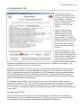
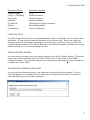
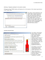
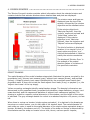
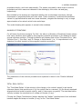
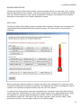
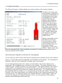
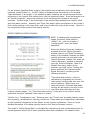
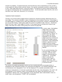
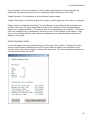
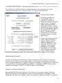
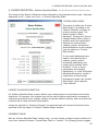
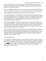
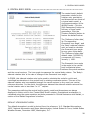
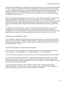
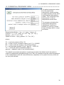
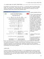
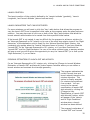

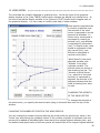
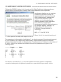
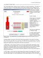
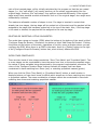

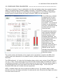
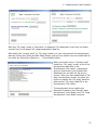
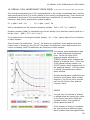

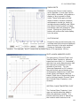
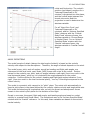
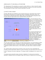
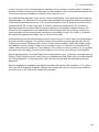
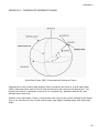
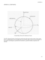
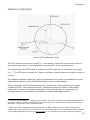


![[en] - User manual, [de] - Betriebshandbuch, [fr]](http://vs1.manualzilla.com/store/data/005845053_1-6d1995608e49c7f1600fcad0c20a630a-150x150.png)