Download Manual and Tutorial

CoCoNUT
Computational Comparative GeNomics Utilities Toolkit
User Manual and Tutorial
Mohamed I. Abouelhoda
August 14, 2008
Contents
1 Introduction
4
1.1
CoCoNUT . . . . . . . . . . . . . . . . . . . . . . . . . . . . . . . . . . . . . . . .
4
1.2
Block-diagram of the system . . . . . . . . . . . . . . . . . . . . . . . . . . . . . .
5
1.3
Manual organization . . . . . . . . . . . . . . . . . . . . . . . . . . . . . . . . . .
5
2 Basic algorithms in CoCoNUT
7
2.1
Basic concepts and definitions . . . . . . . . . . . . . . . . . . . . . . . . . . . . .
7
2.2
The basic chaining problem . . . . . . . . . . . . . . . . . . . . . . . . . . . . . . .
8
2.3
Variation: Chaining multi-chromosomal or draft genomes . . . . . . . . . . . . . . .
10
2.4
Variation: Chaining for cDNA mapping . . . . . . . . . . . . . . . . . . . . . . . .
10
2.5
Variation: Chaining for finding repeats and large segmental duplications . . . . . . .
11
2.6
The alignment step . . . . . . . . . . . . . . . . . . . . . . . . . . . . . . . . . . .
11
2.7
Post-processing: finding syntenic regions . . . . . . . . . . . . . . . . . . . . . . .
12
2.8
Post-processing: clustering cDNAs and finding repeated genes . . . . . . . . . . . .
13
3 Installation and system requirements
14
3.1
System requirements . . . . . . . . . . . . . . . . . . . . . . . . . . . . . . . . . .
14
3.2
Installation . . . . . . . . . . . . . . . . . . . . . . . . . . . . . . . . . . . . . . .
14
3.2.1
Pre-compiled version . . . . . . . . . . . . . . . . . . . . . . . . . . . . . .
14
3.2.2
Another architecture or installation problem . . . . . . . . . . . . . . . . . .
14
3.2.3
Testing Installation . . . . . . . . . . . . . . . . . . . . . . . . . . . . . . .
16
3.3
The config file . . . . . . . . . . . . . . . . . . . . . . . . . . . . . . . . . . . . . .
17
3.4
Files and directory structure . . . . . . . . . . . . . . . . . . . . . . . . . . . . . .
17
3.5
Test data . . . . . . . . . . . . . . . . . . . . . . . . . . . . . . . . . . . . . . . . .
18
4 CoCoNUT in a nutshell: Exploring the main functions
4.1
Comparing finished genomes . . . . . . . . . . . . . . . . . . . . . . . . . . . . . .
1
19
19
4.2
4.3
4.4
4.1.1
Test data . . . . . . . . . . . . . . . . . . . . . . . . . . . . . . . . . . . .
19
4.1.2
Main options of CoCoNUT . . . . . . . . . . . . . . . . . . . . . . . . . . .
20
4.1.3
Calling CoCoNUT . . . . . . . . . . . . . . . . . . . . . . . . . . . . . . .
20
4.1.4
Ouput files . . . . . . . . . . . . . . . . . . . . . . . . . . . . . . . . . . .
21
Comparing draft/ multi-chromosomal genomes . . . . . . . . . . . . . . . . . . . .
24
4.2.1
Test data . . . . . . . . . . . . . . . . . . . . . . . . . . . . . . . . . . . .
24
4.2.2
Main options of CoCoNUT . . . . . . . . . . . . . . . . . . . . . . . . . . .
24
4.2.3
Calling CoCoNUT . . . . . . . . . . . . . . . . . . . . . . . . . . . . . . .
24
4.2.4
Output files . . . . . . . . . . . . . . . . . . . . . . . . . . . . . . . . . . .
25
Repeat analysis . . . . . . . . . . . . . . . . . . . . . . . . . . . . . . . . . . . . .
26
4.3.1
Test data . . . . . . . . . . . . . . . . . . . . . . . . . . . . . . . . . . . .
26
4.3.2
Main options of CoCoNUT . . . . . . . . . . . . . . . . . . . . . . . . . . .
26
4.3.3
Calling CoCoNUT . . . . . . . . . . . . . . . . . . . . . . . . . . . . . . .
27
4.3.4
Output files . . . . . . . . . . . . . . . . . . . . . . . . . . . . . . . . . . .
27
cDNA mapping . . . . . . . . . . . . . . . . . . . . . . . . . . . . . . . . . . . . .
28
4.4.1
Test data . . . . . . . . . . . . . . . . . . . . . . . . . . . . . . . . . . . .
28
4.4.2
Main options of CoCoNUT . . . . . . . . . . . . . . . . . . . . . . . . . . .
28
4.4.3
Calling CoCoNUT . . . . . . . . . . . . . . . . . . . . . . . . . . . . . . .
29
4.4.4
Output files . . . . . . . . . . . . . . . . . . . . . . . . . . . . . . . . . . .
29
5 Comparison of finished genomes
32
5.1
Calling CoCoNUT . . . . . . . . . . . . . . . . . . . . . . . . . . . . . . . . . . .
32
5.2
The parameter file . . . . . . . . . . . . . . . . . . . . . . . . . . . . . . . . . . . .
34
5.3
The fragment generation phase . . . . . . . . . . . . . . . . . . . . . . . . . . . . .
35
5.3.1
The fragment generation parameters . . . . . . . . . . . . . . . . . . . . . .
36
5.3.2
The choice of the fragment generation program . . . . . . . . . . . . . . . .
36
The chaining parameters, and the program CHAINER . . . . . . . . . . . . . . . . .
37
5.4.1
The input and output files for the chaining step . . . . . . . . . . . . . . . .
38
5.4.2
The chaining parameters and the recursive chaining option . . . . . . . . . .
40
5.5
The alignment parameters, and the program alichainer . . . . . . . . . . . . . . . .
41
5.6
The synteny parameters, and the program chainer2permutation.x . . . . . . . . . . .
44
5.6.1
The input and output files . . . . . . . . . . . . . . . . . . . . . . . . . . .
45
5.7
The 2D plots . . . . . . . . . . . . . . . . . . . . . . . . . . . . . . . . . . . . . .
46
5.8
Summary of output files . . . . . . . . . . . . . . . . . . . . . . . . . . . . . . . . .
47
5.9
Tutorial: Comparison of three genomes . . . . . . . . . . . . . . . . . . . . . . . .
48
5.4
2
6 Pairwise comparison of multi-chromosomal and draft genomes
54
6.1
Calling CoCoNUT . . . . . . . . . . . . . . . . . . . . . . . . . . . . . . . . . . .
55
6.2
The parameter files . . . . . . . . . . . . . . . . . . . . . . . . . . . . . . . . . . .
57
6.3
The fragment and chaining step . . . . . . . . . . . . . . . . . . . . . . . . . . . . .
57
6.4
The alignment parameters, and the program alichainer . . . . . . . . . . . . . . . .
58
6.5
The post-processing phase . . . . . . . . . . . . . . . . . . . . . . . . . . . . . . .
58
6.6
Tutorial: Comparison of two draft (multi-chromosomal) genomes . . . . . . . . . .
58
7 Repeat analysis
64
7.1
Calling CoCoNUT . . . . . . . . . . . . . . . . . . . . . . . . . . . . . . . . . . .
64
7.2
The parameter files . . . . . . . . . . . . . . . . . . . . . . . . . . . . . . . . . . .
65
7.3
The fragment and chaining step . . . . . . . . . . . . . . . . . . . . . . . . . . . . .
65
7.4
The alignment parameters, and the program alichainer . . . . . . . . . . . . . . . .
66
7.5
The post-processing phase . . . . . . . . . . . . . . . . . . . . . . . . . . . . . . .
66
7.6
Tutorial: Detecting the large segmental duplications of the Arabidopsis chromosome I
66
8 cDNA/EST Mapping
69
8.1
Calling CoCoNUT . . . . . . . . . . . . . . . . . . . . . . . . . . . . . . . . . . .
69
8.2
The parameter file . . . . . . . . . . . . . . . . . . . . . . . . . . . . . . . . . . . .
71
8.3
The fragment generation and the chaining steps . . . . . . . . . . . . . . . . . . . .
71
8.4
The alignment step . . . . . . . . . . . . . . . . . . . . . . . . . . . . . . . . . . .
72
8.5
Tutorial: Mapping cDNA database to a genomic sequence . . . . . . . . . . . . . .
75
3
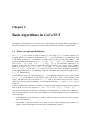
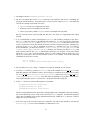
Chapter 1
Introduction
1.1 CoCoNUT
CoCoNUT is a software system for performing the following comparative genomics tasks:
1. Finding regions of high similarity (candidate regions of conserved synteny) among two or multiple genomes, and aligning them.
2. Comparison of two multi-chromosomal or two draft genomes (a draft genome is not a single
sequence but it is a set of sequences called contigs); the current version handles at most two
such genomes.
3. finding repeated segments in large genomic sequences.
4. Mapping a cDNA/EST database to a large genomic sequence.
To cope with the large genomic sequences, CoCoNUT is based on the anchor-based strategy that is
composed of three phases:
1. Computation of fragments (similar regions among genomic sequences).
2. Computation of highest-scoring chains of colinear fragments. Each of these highest-scoring
chains corresponds to a region of similarity. The fragments in each of such chains are the
anchors.
3. Alignment of the regions between the anchors of a chain by using standard dynamic programming.
The fragments we use are computed using the Vmatch package, which is based on an efficient data
structure called the enhanced suffix array. The wide variety of applications CoCoNUT can be used
for is attributed to the number of variations of the chaining step. Our program CHAINER carries out
the chaining step in our system. It includes various variations of the chaining algorithm to solve the
above mentioned different tasks.
The third phase of the anchor-based strategy finalizes the comparison by computing an alignment
on the character level. For comparing two genomes or repeat analysis, CoCoNUT uses a traditional sequence alignment algorithm. For comparing multiple genomes, a wrapper of the program
4
CLUSTALW is used. For cDNA mapping, we use a variation of the standard dynamic programming
algorithm, where the splice site signals and the gene structure are taken into account.
In CoCoNUT, there are further options to post-process the resulting chains (aligned chains). For
example, when comparing genomic sequences, we can detect the syntenic regions and report permutations for these regions. These permutations can then be input to a another program to compute a
rearrangement scenario. Another example of post-processing is the clustering of cDNAs aligned to
the same locus. This option enables to study variants of the genes produced by alternative splicing.
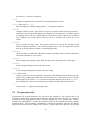
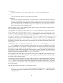
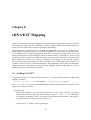
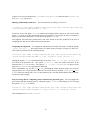
1.2 Block-diagram of the system
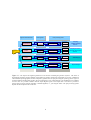
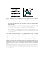
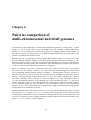
The block diagram in Figure 1.1 layouts how the CoCoNUT system works. It shows the three phases
of the anchor-based strategy along with some extra post-processing options specific to each comparative task. The user has a full control over each process. For example, one can compute chains,
visualize them and end the comparison. One can also detect syntenic regions without computing an
alignment, to speed up the comparison. More details about these steps are given in the following
chapters when discussing each of these tasks. Our system is so modular that any programs or scripts
can be easily modified, extended, or replaced with other modules without affecting the remaining
parts of the system. For instance, the user can replace the Vmatch package with any other program
(e.g., BLASTZ) provided that the input has the format used in the system. The user can also replace
or modify some scripts of the system depending on his needs.
In fact, the user can compare two finished genomes through running either the the task of comparing
two genomes or the task of comparing multiple genomes. However, the constraints on fragments will
limit the choice to one task; this will be explained in Chapter 6.
1.3 Manual organization
This manual is organized as follows. In Chapter 2, we introduce formal definitions of fragments
and chains. The installation and system requirements of CoCoNUT are given in Chapter 3. Chapter
4 briefly describes and navigates through the basic functionalities of CoCoNUT. In Chapter 5, we
handle the task of comparing multiple genomic sequences. Chapter 6 addressed the task of comparing
two multi-chromosomal or two draft genomic sequences. In Chapter 7, we show how CoCoNUT is
used to analyze repeated sequences and to detect large segmental duplications. The task of mapping a
cDNA/EST database to a genomic sequence is is handled in Chapter 8.
5
Fragment Generation Phase
Chaining Phase
Post−processing Phase
Visualization
Multimat/ramaco
CHAINER
Detailed Alignment
Synteny
local chaining
Visualization
> gi genome 1
GCCGCGCGT
CGGT
CG..
Vmatch
CHAINER
Vmatch
Genomes
Comparing two draft or
two multi−chromosomal
Detailed Alignment
Synteny
local chaining for contigs
Comparing
Multiple Finished
Genomes
Visualization
CHAINER
Detailed Alignment
cDNA Mapping
cDNA Clustering
chaining for cDNAs
Visualization
Vmatch
CHAINER
Repeat Analysis
Detailed Alignment
Synteny
local chaining for repeats
Figure 1.1: The input to the fragment generation tool are the files containing the genomic sequences. The choice of
the fragment generation program depends on the number of genomes and the type of fragments to be used. CHAINER is
called with the options appropriate for each comparative genomic task. The post-processing for reporting syntenic regions is
useful for multiple-chromosomal genomes, but it is meaningless in case of draft genomes. The feedback arrows symbolize
recursive calls: It is possible to further chain the output aligned regions or the output chain. Note that it is possible to
perform post-processing without computing a detailed alignment, i.e., just using the chains. The post-processing options
depends on the comparison task carried out.
6
Chapter 2
Basic algorithms in CoCoNUT
To completely understand how our system work, we present here some details about the algorithms in
our system and how they are used to solve the previously mentioned comparative genomic tasks.
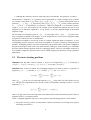
2.1 Basic concepts and definitions
For 1 ≤ i ≤ k, let Si denote a string of length |Si |. The string Si [1..n] is a DNA sequence or a
complete genome of n characters (nucleotides). Si [li . . . hi ] is the substring of Si starting at position
li and ending at position hi . A fragment is a similar region occurring in the given genomes. This
region is specified by the substrings S1 [l1 . . . h1 ], S2 [l2 . . . h2 ], . . . , Sk [lk . . . hk ]. A fragment is called
exact if S1 [l1 . . . h1 ] = S2 [l2 . . . h2 ] = . . . = Sk [lk . . . hk ], i.e., the substrings composing it are
identical. In this case, one speaks of fragments of the type multiple exact match. Such a match is
called left maximal, if Si [li − 1] 6= Sj [lj − 1], for some i 6= j, and it is called right maximal if
Si [hi + 1] 6= Sj [hj + 1], for some i 6= j. A maximal multiple exact match, denoted by multi-MEM,
is left and right maximal, i.e., the substrings cannot be extended to the left and to the right in all Si ,
1 ≤ i ≤ k, simultaneously.
A multi-MEM is called rare if the substring Si [li . . . hi ] composing it appears at most r times in each
Si , 1 ≤ i ≤ k. In this manual, we will call the value r the rareness value. A multi-MEM is called
unique, and abbreviated by multi-MUM, if r = 1. That is, the famous maximal unique matches
(MUMs) used in the program MUMmer are multi-MEMs such that r = 1 and k = 2 (i.e., for two
sequences).
If character mismatches, deletions, or insertions are allowed in the substrings composing the fragment,
then we speak of a non-exact fragment; i.e., S1 [l1 . . . h1 ] ≈ S2 [l2 . . . h2 ] ≈ . . . ≈ Sk [lk . . . hk ].
Our system can basically use any kind of fragments, provided that they are output in the adopted CoCoNUT format. However, we use (rare) multi-MEMs as the default fragments in our system because
of the following:
• multi-MEMs are easier and faster to compute, and because they can achieve accuracy comparable to other matches.
• The number of non-exact matches is too high to process when comparing large genomic sequences, which might require extremely large computational resources.
7
• Although the sensitivity increases when using non-exact matches, the specificity is reduced.
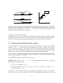
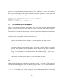
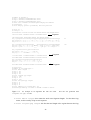
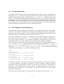
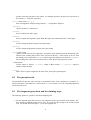
Geometrically, a fragment f of k genomes can be represented by a hyper-rectangle in Rk with the
two extreme corner points beg(f) and end(f). beg(f)= (l1 , l2 , . . . , lk ), where the fragment starts at
positions l1 , . . . , lk in S1 . . . Sk respectively, and end(f)= (h1 , h2 , . . . , hk ), where it ends at positions
h1 , . . . , hk in S1 . . . Sk respectively; see Figure 2.1. With every fragment f , we associate a positive
weight f.weight ∈ R. This weight can, for example, be the length of the fragment (in case of exact
fragments) or its statistical significance. In our system, we use the fragment length as the defualt
fragment weight.
We also define two imaginary points 0 = (0, . . . , 0) (the origin) and t = (|S1 |, . . . , |Sk |) (the terminus) as imaginary fragments with weight 1. In some output files in CoCoNUT, the origin point might
be reported; it is done for ease of computations.
The program CHAINER is used on our system to compute significant chains of fragments. In case
of comparing genomic sequences, each chain corresponds to a region of similarity among the given
genomes. In mapping cDNAs, each chain corresponds to the position where each cDNA is mapped in
the genome and it gives a hint on the exon-intron structure of the gene. In the following, we will handle
the more general chaining problem used for comparing genomes. Then we will handle variations of
it for another comparative genomic tasks, such as cDNA mapping and detection of large-segmental
duplications.
2.2 The basic chaining problem
Definition 2.2.1 We define a binary relation ≪ on the set of fragments by f ≪ f ′ if and only if
end(f).xi < beg(f ′ ).xi for all 1 ≤ i ≤ k. If f ≪ f ′ , we say that f precedes f ′ .
Definition 2.2.2 A chain of colinear non-overlapping fragments (or chain for short) is a sequence of
fragments f1 , f2 , . . . , fℓ such that fi ≪ fi+1 for all 1 ≤ i < ℓ. The score of C is
score(C) =
ℓ
X
fi .weight −
ℓ−1
X
g(fi+1 , fi )
i=1
i=1
where g(fi+1 , fi ) is the cost of connecting fragment fi to fi+1 in the chain. We will call this cost gap
cost. The gap cost implemented in the current version of CHAINER is defined as follows. For two
fragments f ≪ f ′ ,
g(f ′ , f ) =
k
X
|beg(f ′ ).xi − end(f ).xi |
i=1
That is, the gap cost between two fragments is the distance between the end and start point of the two
fragments in the L1 (rectilinear) metric.
Given n weighted fragments from two or more genomes, the following problems can be defined:
• The global chaining problem is to determine a chain of maximum score starting at the origin 0
and ending at terminus t.
8
1
S1
4
2
5
7
t
S2
6
3
7
4
5
1
S2
3
2
3
7
6
2
o
(a)
(b)
S1
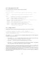
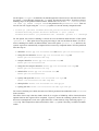
Figure 2.1: The fragments in (a) can be represented by (hyper-) rectangles in a space with dimension
equals the number of genomes, and each axis corresponds to one genome, as shown in (b). Given a
set of fragments, an optimal global chain of colinear non-overlapping fragments (left figure) starts and
ends with two imaginary fragments of weight equals one: O and t.
Such a chain will be called optimal global chain. Figure 2.1 shows a set of fragments and an
optimal global chain.
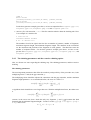
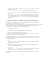
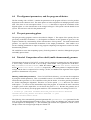
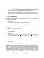
• The local chaining problem is to determine a chain of maximum score ≥ 0. Such a chain will
be called optimal local chain. It is not necessary that this chain starts with the origin or ends
with the terminus. Figure 2.2 shows a set of fragments and an optimal local chain.
• Given a threshold T , the all significant local chains problem is to determine all chains of score
≥ T . It is easy to see that the all significant local chains problem is the generalization of the
local chaining problem.
In local chaining, some chains can share one or more fragments composing a cluster of fragments.
In the example of Figure 2.2, the local chains {1, 3, 6} and {1, 4, 6} share the fragment 1 and make
up a cluster of the fragments {1, 3, 4, 6}. The cluster {7, 8, 9} contains two local chains {7, 8} and
{7, 9}. To reduce the output size, we report the clusters and from each cluster we report a local chain
of highest score as a representative chain of this cluster. This representative chain is a significant local
chain. In the example of this figure two chains are reported: {1, 4, 6} and {7, 8}. The fragments {2}
and {5} in the figure are chains of one fragment. They would be reported if their score is ≥ T .
CHAINER uses techniques from computational geometry to solve the chaining problems. These techniques are based on orthogonal range search for maximum, which is implemented in CHAINER using
an optimized version of kd-tree [4]. For more algorithmic aspects of CHAINER and these techniques,
see [1–3].
The user can constrain the gap length between the fragments, which is achieved by limiting the region
of the range queries. In other words, no two fragments can be connected in a chain if the number of
characters separating them exceeds a user-defined threshold. This option prevents unrelated fragments
from extending the chain.
9
g
1
4
3
1
5
7
8
t
g
2
6
2
6
9
4
3
1
g2
1
4
6
7
8
8
9
5
7
2
o
(a)
(b)
g
1
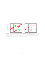
Figure 2.2: Computation of an optimal local chain of colinear non-overlapping fragments. The optimal local chain is composed of the fragments 1, 4, and 6. The local chains {1, 3, 6} and {1, 4, 6}
share the fragment 1 and make up a cluster of the fragments {1, 3, 4, 6}. The representative chain of
this cluster is the chain {1, 4, 6}. The chain {7, 8} is a representative chain of the cluster {7, 8, 9}.
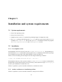
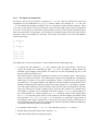
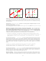
2.3 Variation: Chaining multi-chromosomal or draft genomes
A multi-chromosomal genome is a genome composed of multiple chromosomes. Each chromosome is
represented by a string. A draft genome is not a single sequence (string), but it is a set of subsequences
of the genome (substrings) called contigs. Both draft or multi-chromosomal genome are usually given
by multiple-fasta files. Comparing draft or multi-chromosomal genomes is to find local chains such
that the chains are not crossing the borders between the contigs (chromosomes). This is because
two consecutive contigs (chromosomes) in the input file are not necessarily adjacent to each other in
the genome. Therefore, we variate the local chaining procedure, by limiting the region of the range
queries, to meet this requirement. Figure 2.3 shows an example of two draft (or multi-chromosomal)
genomes compared to each other.
2.4 Variation: Chaining for cDNA mapping
Mapping cDNA/EST to a genomic sequence is to find the region in a genomic sequence, from which
the cDNA/EST stems from. This is also a variation of the local chaining problem, where (1) gap costs
are not considered (gaps correspond to non-coding introns), (2) overlaps between the fragments of a
chain are allowed. It was observed that the fragments usually overlap at the exon-intron boundaries.
Allowing overlapping fragments in a chain (while subtracting the amount of overlap from the objective
function) improves the chain coverage and reduces the running time. More details about this algorithm
is given in [8].
10
draft genome 2
c23
c22
c21
c11
c12
c13
draft genome 1
Figure 2.3: The contigs (chromosomes) c11 , c12 and c13 of the first draft (multi-chromosomal) genome
are compared to the contigs (chromosomes) c21 , c22 and c23 of the second genome. The fragments of
each chain must come from only two contigs (chromosomes), i.e., the chain cannot cross any border
between two contigs (chromosomes). The range maximum query is limited to contig (chromosome)
boundaries to satisfy this constraint.
2.5 Variation: Chaining for finding repeats and large segmental duplications
For repeat analysis, the fragments are of the type maximal repeated pairs. Formally, the substrings
S[l1 . . . h1 ] and S[l2 . . . h2 ] correspond to a repeated pair whose first occurrence is in the region
[l1 . . . h1 ] and whose second occurrence is in the region [l2 . . . h2 ]. These fragments can also be
regarded as maximal exact matches obtained by comparing the genome to itself. The fragments can
also be represented in a 2D space such that the x- and y-axis correspond to the same genome. To
avoid redundancy, we assume that l1 < l2 , which also implies that h1 < h2 . Figure 2.4 shows an
example of fragments and their 2D representation. The chaining algorithm for handling repeats works
exactly like the algorithm for local chaining but with one extra constraint. Let [xl ..xr ] and [yl ..yr ]
be the chain boundaries corresponding to the first and second occurrence of the repeated segment.
Then, we restrict that xr < yl . In Figure 2.4 (a), we show a chain composed of the fragments f1
and f2 and f3 . The fragment f4 cannot be appended to this chain because it would cause an overlap
of the regions bounding the two occurrences of the repeat. For palindromic repeats, where the chain
is constructed from fragments from the positive strand and the negative strand, this restriction is automatically satisfied. That is for palindromic repeats (chains), we use the same algorithm for local
chaining.
2.6 The alignment step
The alignment step in our system is carried out by the programs alichainer and estchainer. The former
is used for genomic sequences, and the latter is used for cDNA/EST sequences.
The program alichainer applies a standard dynamic programming algorithm between the regions of
the fragments of each chain. For two genomes, we use a built-in code. For multiple genomes we use
11
f4
S
f1
S
f2
f4
f4
f3
f1
f2
f3
f3
(a)
f2
f1
S
f1
f2
f3
f4
S
S
(b)
(c)
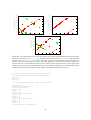
Figure 2.4: (a) The fragments are repeated pairs and in (b) they are represented as if we compare the
genome to itself. (c) 2D plot of the fragments. Note that the fragments appear only in one octant
(the region bounded by the lines x = 0 and y − x = 0), because we have the constraint that the first
occurrence of the repeat is before the second one.
a wrapper of the CLUSTALW program.
The program estchainer uses a variation of the dynamic programming algorithm to align the regions
between the fragments of a chain. estchainer takes into account (1) the splice-site signals (the canonical ones or those described by a Position Weight Matrices), and (2) the exon-intron structure.
2.7 Post-processing: finding syntenic regions
Two similar regions are called syntenic if they are directly following one another in the compared
genomes. Let B1 , ..., Bt denote the regions of high similarity among k genomes. In the sequel,
we also call these regions blocks. The blocks can be the chains output from CHAINER or, the chains
output from alichainer such that their alignments have percentage identities that exceed a user-defined
threshold, or as we will see, the chains obtained by a recursive chaining over the chains.
Let beg(bi ) and end(bi ) denote the points where bi starts and ends in the given genomes, respectively.
Let w(bi )Pdenote a function that assigns a weight to each block. As default in our system we take
w(bi ) = kj=1 (end(bi ).xj − beg(bi ).xj ).
The synteny determination problem is defined as follows:
Definition 2.7.1 Given the set B = {b1 , . . . , bt } of local alignments, find a subset B ′ ⊆ B such that
the following two conditions hold:
1.
P|B′ |
i=1 w(bi )
is maximum, bi ∈ B ′ .
2. For any two regions b′ , b′′ ∈ B ′ , b′ [beg(b′ ).xj ..end(b′ ).xj ] ∩ b′′ [beg(b′′ ).xj ..end(b′′ ).xj ] = ∅,
for all dimensions 1 ≤ j ≤ k.
This problem is known in the literature as the Maximum Independent Set, which is NP-complete.
Therefore, we use a heuristic method to find a set of non-overlapping blocks with score as high
12
as possible. For this purpose, we use 1D chaining algorithm iteratively w.r.t. each dimension. Let
B ′ = {b1 , . . . , bt } denote the blocks in an optimal 1D chain from k genomes w.r.t. dimension xj . The
score of this chain is
t
X
(end(b′i ).xj − beg(b′i ).xj )
i
It is clear that after each iteration i, done w.r.t. genome i, no two blocks in the resulting chain are
overlapping in genome i. Because we choose the chain with the highest possible score, we obtain
good solution to the problem. In CoCoNUT, the program chainer2permutation.x is an implementation
of this algorithm.
The program chainer2permutation.x has some options and variations that are of practical use for
biological data. The program can filters out repeats, and allow a little overlapping between the blocks.
Filtering repeats is useful because some genomes are highly repetitive, and filtering repeats before the
1D chaining is useful to report better results. Allowing overlaps in the chains aims at overcoming any
drawback in the method for determining the blocks. In other words, the boundaries of the block might
be mistakenly flanked to the left or the right.
2.8 Post-processing: clustering cDNAs and finding repeated genes
In CoCoNUT, the program estchainer2cluster is use to carry out this task. The program
detects repeated genes by inspecting if each cDNA has multiple chains mapped to different loci in
the genomic sequences. It clusters the genes by collecting for each loci, the genes mapped to it. This
module is straightforward and requires just to sort the output chains: once w.r.t. their number in the
cDNA file and once w.r.t. their position in the genome.
13
Chapter 3
Installation and system requirements
3.1 System requirements
• Linux-Unix operating system.
• Perl (at least version v5.8.1).
• Gnuplot (at least version 3.7), optional for producing images of comparison results.
• The Vmatch package with the programs multimat and ramaco (previously called memspe),
available at www.vmatch.de. (Be sure that your Vmatch distribution contains the programs
mkrcidx, vseqinfo, mkvtree, and vsubseqselect, as well.)
3.2 Installation
3.2.1 Pre-compiled version
The distributed version of CoCoNUT is the file CoCoNUT.distrib.tar.gz. The distributed version includes the Vmatch and multimat (the program ramaco is distributed with multimat) package
is pre-compiled for Linux 32bit, Linux 64bit machines, and for for MAC OS.
To have CoCoNUT running, first decompress this file using the following command
> gzip -cd CoCoNUT.distrib.tar.gz | tar xvf The destination directory of the system is called CoCoNUT.distrib. It is then recommended to
download the test data and put it in the CoCoNUT directory. Then run the test script TestScript.pl
to check your installation; see Subsection 3.2.3.
If there is a problem or you have another architectures, read the next section.
3.2.2 Another architecture or installation problem
If there is a problem or you have another architecture, then proceed as follows:
14
1. Decompress the file CoCoNUT.distrib.tar.gz.
2. Be sure you obtain the correct Vmatch package with multimat and ramaco (including the
programs specified above). Note that ramaco was previously called memspe. The following
versions are already tested with CoCoNUT.
• Vmatch version 2.0, compiled in July 2007.
• multimat version 2.0 compiled in June 2007.
• ramaco (previously called memspe) version 2.0 compiled in June 2007.
Recent versions can be used provided that they have the same set of arguments and output
formats.
3. It is recommended to put the decompressed Vmatch and multimat packages in the directory bin. (Note that ramaco is distributed with multimat). I.e., now we have the directories
bin/multimat.distrib and bin/vmatch.distribution within the CoCoNUT directory; see Section 3.4 for more details about the CoCoNUT directory structure. Alternatively,
you can set the config file as explained in Section 3.3. Another easy way is as follows:
In the distribution, you have the two files: config.i686-pc-linux-gnu-32-bit and
config.i686-apple-darwin-32-bit. Rename one of them to be called config, and
then reset the paths to the Vmatch and multimat packages; see Section 3.4 for more details
about the config file. In the distributed version, we use symbolic links to point to the config file we would like to use over the machine we have. For example, we used the following
commands for the Linux version:
>rm -f config
>ln -s config.i686-pc-linux-gnu-32-bit config
4. Be sure that your cc, gcc, and g++ compilers are properly installed in your system
5. Go to the src directory, open the Makefile, and set the variable MACHINE OS BITS to the
path that matches your installed version. Do not forget to comment out or delete the two lines
MACHINE OS BITS=i686-pc-linux-gnu-32-bit and the line MACHINE OS BITS=
i686-apple-darwin-32-bit. Note that this line should be in accordance with the content of the config file you use, see Section 3.3 for details about the config file.
6. In the src directory, run the following three commands
CoCoNUT.distrib/src> make clean
CoCoNUT.distrib/src> make
CoCoNUT.distrib/src> make install
The first command deletes the object files, which might not be compatible with your machine,
the second builds the source code of the CoCoNUT C/C++ programs, and the third program
copies the executables in the proper destination directories within the bin directory, which is
under the CoCoNUT directory.
7. Now move up to the CoCoNUT directory, install the test data in this directory, and run the
TestScript.pl to test your installation; see Subsection 3.2.3.
15
For successful running, we recommend that you do not change the directory structure of the system.
Moreover, CoCoNUT must be called while being in its directory.
The main program interface coconut.pl exists in the coconut directory. In addition, you will
find the config file, where you can specify the location of the Vmatch package, as will be explained
in Section 3.3.
64bit version
For 64bit machines, write open the Makedef file and replace the line ”WORDSIZE=-m32” with
”WORDSIZE=-m64”. Note that the line ”WORDSIZE=-m32” is originally commented out so that
you can use your default settings, and as it might cause problem with some settings, please restore it
back if it matches your settings. To compile, run the three commands
CoCoNUT.distrib/src> make clean
CoCoNUT.distrib/src> make
CoCoNUT.distrib/src> make install
For further setting specific to your machine, you have to edit the Makedef file in the source directory.
3.2.3 Testing Installation
Install the test data from the CoCoNUT web site and decompress it in the CoCoNUT directory. Then
run the script TestScript.pl to test your installation.
Usage: TestScript.pl [options]+
-multiple
-pairwise
-map
-repeat
-->
-->
-->
-->
test
test
test
test
compare two or more finished genomes
compare two finished or draft genomes
map a cdna library to a genomic sequence
find repeats in a genomic sequences
-all
--> test all the CoCoNUT
tasks
-v
--> verbose mode, show intermediate steps
Example:
> TestScript.pl -all
This script checks the installed packages and runs the examples given in Chapter 4. This might take
sometime, but it is a useful test. After the successful completion of the test, it is recommended to
open the output files in the destination directory and display the output; see Chapter 4 for exploring
and testing all CoCoNUT functionalities.
Further compilation options
For any further compilation options you would like to use or for any options to modify, edit the
Makedef file in the directory src, and recompile the sources using the three commands given above.
16
3.3 The config file
The config file contains the paths for the programs needed for the system. Below we show the default
config file. The lines separated by # are comment lines. The line starting with “FRAGMENT=”
specifies the path to the Vmatch package. The line starting with “FRAGMENT MULT” specifies the
path to the programs ramaco and multimat. Each specified directory should contain the associated
programs distributed with multimat and ramaco. The line starting with “CHAINING=” specifies the
path to the programs CHAINER, chainer2permutation.x, and other programs for format transformation. The line starting with “ALIGN=bin/align” specifies the path to the program alichainer.
# PATHS
#fragment generation directory for the program vmatch
FRAGMENT=bin/vmatch.distribution
#fragment generation directory for program multimal/ramaco
FRAGMENT_MULT=bin/multimat_ramaco.distrib
#chaining directory
CHAINING=bin/chainer
#align directory
ALIGN=bin/align
3.4 Files and directory structure
The system has the following directory structure:
• bin : This directory contains the following four sub-directories 1) vmatch.distribution,
2) multimat_ramaco.distrib, 3) chainer, and 4) align. The first one contains
programs from the Vmatch. The second one contains programs from the multimat/ramaco
package (ramaco was previously called memspe). Programs in both directory are used to
compute the fragments. Collectively, these programs are: mkrcidx, vseqinfo, mkvtree,
multimat, ramaco, vmatch, and finally vsubseqselect. These programs will be distributed according to a license at www.vmatch.de. If Vmatch is already installed on your
system, we recommend that you copy these programs to these two directories. Otherwise, you
might carefully re-edit the config file. The chainer directory contains the CHAINER program
for computing the chains and other programs for format transformation and post-processing.
The align directory contains programs for computing alignments on the character level given
the chains produced by the program CHAINER.
• finalscripts: This directory contains Perl’s scripts for performing deferent comparative
genomic tasks. These scripts encapsulate the programs in the bin directory. This directory includes four sub-directories: comp_finished, comp_pairwise, map_cdna, and
repeat. The first one includes scripts for comparing multiple finished genomes. The second
includes scripts for comparing pairwise draft or finished genomes. The third includes scripts
for mapping cDNA sequences. The fourth contains scripts for repeat analysis.
17
• src: This directory contains source code for CHAINER and the post-processing modules
align_cdna_mod (for aligning the cDNAs given chains), cdna_postprocessing (for
clustering cDNAs and reporting repeated genes), find_permutations (for computing syntenic regions and filtering repeats in genomes), filter_alignment (for filtering alignments
with score less than a certain threshold), and finally align_module_draft (for aligning
genomes given chains). The sources of the Vmatch package are not included.
3.5 Test data
Test data can be downloaded from the system web-page. We have supplied some data to demonstrate
our system. In this manual we will assume that the test data directory exists in the CoCoNUT.distrib
directory. The test data directory contains the following directories:
• ecoli shig: contains the three fasta files NC 000913.fasta, NC 007384.fasta, and
NC 007613.fasta containing the three bacterial genomes Escherichia coli Shigella sonnei
Ss046, and Shigella boydii Sb227, respectively.
• chlamd: contains the three files AE001273.fasta, AE001363.fasta, and AE002160.fasta
containing the three bacterial genomes Chlamydia trachomatis, Chlamydia pneumoniae, and
Chlamydia muridarum, respectively.
• draft: contains two directories artificial and yeast The former contains the two files
NC_002745.fna.draft.shuffled and NC_003923.fna. draft.shuffled containing shuffled contigs from the genomes Staphylococcus aureus subsp. aureus N315 and
Staphylococcus aureus subsp. aureus MW2, respectively. The latter directory contains the
two files yeast genome, which contains the finished multi-chromosomal genome of S. cerevisiae, and s.paradoxus.scfld, which contains the 333 scaffolds of the draft genome of
S. paradoxus (assembled from 832 contigs; see [5, 7]).
• cdna: contain the directory Arabidposis, which contains the two files cdna1.seq and
chrom1.seq. The first contains cDNA sequences from Arabidopsis thaliana. The second is
Chromosome I of the Arabidopsis genome.
• repeat: contains the directory Arabidposis, which contains Chromosome I of the Arabidopsis genome.
18
Chapter 4
CoCoNUT in a nutshell: Exploring the
main functions
The objective of this chapter is to test your installation and to explore the main functionalities of
CoCoNUT. We will briefly investigate some of the output files to ascertain the correct installation. We
will use the program default estimated parameters, which might not be the best. More on parameter
tuning is addressed in detail in the following sections. (Briefly this is done by re-editing the parameter
file and passing it to CoCoNUT.)
By calling CoCoNUT without parameters, you will obtain the following.
> coconut.pl
Usage: coconut.pl -task_name arguments
task_name: -multiple
-pairwise
-map
-repeat
-->
-->
-->
-->
compare two or more finished genomes
compare two finished or draft genomes
map a cdna library to a genomic sequence
find repeats in a genomic sequences
To view arguments for each task, run coconut.pl with task_name
Example:
> coconut.pl -multiple
This means that you have to specify the task you want to accomplish and pass in addition the arguments and input data. In the following, we will explore the aforementioned four tasks.
4.1 Comparing finished genomes
.
4.1.1 Test data
We use the three bacterial genomes Chlamydia trachomatis (AE001273.fasta), Chlamydia pneumoniae (AE001363.fasta), and Chlamydia muridarum (AE002160.fasta). (These are also in
the test data distributed with CoCoNUT). We assume that these data are in the testdata/chlamd
directory within the CoCoNUT directory.
19
4.1.2 Main options of CoCoNUT
To see the main options of this task, run the following command.
> coconut.pl -multiple
Usage: perl coconut.pl
Arguments:
-fp
Options:
-pr
-v
-forward
-align
-plot
-plotali X
-indexname
-useindex
-usematch
-usechain
-usealign
-prefix
-syntenic
-fp multimat|ramaco
<Options>
seq_1 seq_2 <seq_3> ... <seq_k>
: fragmnet generation prog. Specify either multimat or ramaco
:
:
:
:
:
:
:
:
:
:
:
:
:
parameter file (optional), if not given defaults are computed
verbose mode, i.e., deisplay of the program steps
run the comparison for forward strands only
compute alignment using clustalw
produce Postscript 2D plots of the chains
filter out alignments with idenetity < X (0< X <= 1) and produce 2D plots
specify the index if constructed
do not construct index again
do not compute matches again, this construct no index
use the computed chains and complete processing.
use the computed alignments and complete processing
specify a prefix name for the output files
computes sysntenic regions by removing repeats and applying
1D chaining over all dimensions.
4.1.3 Calling CoCoNUT
To find similar regions in the three aforementioned genomes, run CoCoNUT as follows.
> coconut.pl -multiple -fp ramaco -v -plot -syntenic \\
testdata/chlamd/AE001273.fasta testdata/chlamd/AE002160.fasta \\
testdata/chlamd/AE001363.fasta
The argument -multiple specifies the task of comparing multiple genomes; the other arguments
and options are specified as follows:
• The argument -fp ramaco specifies that the program ramaco is used to generate the fragments. This program generates fragments of the type rare multi-MEMs.
• The option -v (verbose mode) shows the intermediate steps of CoCoNUT.
• The option -plot produces Postscript 2D plots of the similar regions (chains). The produced
plots are projections of the chains with respect to all pairwise genomes.
The parameters estimated (e.g., minimum fragment length, and maximum gap between fragments) for
comparing these three genomes are stored in the automatically generated file parameters.auto.
You can re-edit the paramters and pass this file to CoCoNUT and run the system again, starting from
the phase with the changed paramters using the options usematch, usechain, or usealign. For
more details about the format of the parameter file, see Section 5.2. The other options are handled in
the tutorial of Chapter 5.
20
4.1.4 Ouput files
The output files have the prefix fragment and they are stored in the directory of the first genome
(the prefix and the destination directory can be changed with the option -prefix, as explained in
Section 5.1). As a result of the above options, the following set of files are generated.
• fragment.ppp, fragment.ppm, fragment.pmp, and fragment.pmm, containing fragments in CHAINER
format. The letter “p” in the extension corresponds to the positive (+) strand, and the letter
“m” corresponds to the negative (−) strand. The file “fragment.ppp” contains fragments from
the positive strands of the three genomes. The file “fragment.ppm” contains fragments from
the positive strands of genomes 1 and 2 and the negative strand of genome 3. The file “fragment.pmp” contains fragments from the positive strands of genomes 1 and 3 and the negative
strand of genome 2. The file “fragment.pmm” contains fragments from the positive strand of
genomes 1 and the negative strands of genomes 2 and 3.
• *.ppp.chn, .ppm.chn, .pmp.chn, and *.pmm.chn files, storing the resulting chains from the
*.ppp, *.ppm,*. pmp and *.pmm fragment files.
• *.ppp.ccn, *.ppm.ccn, *.pmp.ccn, and *.pmm.ccn files, containing the resulting chains for the
respective fragment files, but in compact form for plotting. I.e., just the chain boundaries are
stored, not the fragments of the chains.
• *.dat and *.gp files, used for generating plots using gnuplot.
• *.1x2.gp.ps, *.1x3.gp.ps, and *.2x3.gp.ps, postscript files containing the plot of the chain projection w.r.t. the first and second genome; the first and third genome, the second; and third
genome, respectively.
• *.dat.syn.1x2.gp.ps, *.dat.syn.1x3.gp.ps, and *.dat.syn.2x3.gp.ps, postscript files containing the
plot of the syntenic regions projection w.r.t. the first and second genome; the first and third
genome, the second; and third genome, respectively.
To visualize the output chain with respect to the first and second genome, run
> gv testdata/chlamd/fragment.mm.ccn.1x2.gp.ps
The other projections of the chain are in the files testdata/chlamd/fragment.mm.ccn.1x3.gp.ps
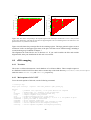
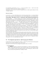
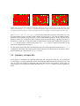
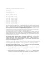
and testdata/chlamd/fragment.mm.ccn.2x3.gp.ps. Figure 4.1 shows the postscript
files for all the three projections.
To visualize the output syntenic regions with respect to the first and second genome, run
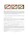
> gv testdata/chlamd/fragment.mm.ccn.dat.syn.1x2.ps
The other projections of the syntenic regions are in the two files testdata/chlamd/fragment.mm.ccn.dat.syn.1x3.gp.ps and testdata/chlamd/fragment.mm.ccn.dat.syn.2x3.gp.ps. Figure 4.2 shows the postscript files for all the three projections.
Note that other files would have been generated, if more post-processing steps had been chosen. For
example, the files containing the alignments on the nucleotide level have not yet been produced,
because no option for producing the alignment was set in the command line.
21
1.4e+06
1.2e+06
1e+06
testdata/chlamd/AE002160.fasta
testdata/chlamd/AE001363.fasta
1.2e+06
1e+06
800000
600000
400000
800000
600000
400000
200000
200000
0
0
0
200000
400000
600000
800000
testdata/chlamd/AE001273.fasta
1e+06
1.2e+06
0
200000
400000
600000
800000
1e+06
1.2e+06
testdata/chlamd/AE001273.fasta
1.2e+06
testdata/chlamd/AE002160.fasta
1e+06
800000
600000
400000
200000
0
0
200000
400000
600000
800000
1e+06
1.2e+06
1.4e+06
testdata/chlamd/AE001363.fasta
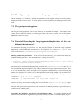
Figure 4.1: Comparison of the three bacterial genomes Chlamydia trachomatis (AE001273.fasta),
Chlamydia pneumoniae (AE001363.fasta), and Chlamydia muridarum (AE002160.fasta). The upper left plot is a projection of the chains with respect to the first (x-axis) and second genomes (y-axis). The
upper right plot is a projection of the chains with respect to the first (x-axis) and third genomes (y-axis). The
lower plot is projection of the chains with respect to the second (x-axis) and third genomes (y-axis). Red lines
are chains between strands with the same orientation and green lines are chains between strands with different
orientations (inversion).
Producing alignment
To produce alignments on the nucleotide level, add the option -align to the aforementioned command line. The produced files would be *.ppp.chn.align, *.ppm.chn.align, *.pmp.chn.align, and
*.pmm.chn.align files, storing the alignment of the respective chains on the nucleotide level. These
files are namely
testdata/chlamd/fragment.mm.pmm.chn.align
testdata/chlamd/fragment.mm.pmp.chn.align
testdata/chlamd/fragment.mm.ppm.chn.align
testdata/chlamd/fragment.mm.ppp.chn.align
Below is a snapshot of the alignment file, where we show the last chain in the alignment file testdata/chlamd/fragment.mm.ppp.chn.align. (Dots in the alignment refers to matching character with
that of the first sequence.) Details of the alignment file format is given in Section 5.5.
# Chain no. 113
# Contigs 1 1 1
# Boundaries: 84:1018109-1018192 84:1175861-1175944 84:293512-293595
22
1.4e+06
1.2e+06
1e+06
testdata/chlamd/AE002160.fasta
testdata/chlamd/AE001363.fasta
1.2e+06
1e+06
800000
600000
400000
800000
600000
400000
200000
200000
0
0
0
200000
400000
600000
800000
testdata/chlamd/AE001273.fasta
1e+06
1.2e+06
0
200000
400000
600000
800000
1e+06
1.2e+06
testdata/chlamd/AE001273.fasta
1.2e+06
testdata/chlamd/AE002160.fasta
1e+06
800000
600000
400000
200000
0
0
200000
400000
600000
800000
1e+06
1.2e+06
1.4e+06
testdata/chlamd/AE001363.fasta
Figure 4.2: The output 2D plots after using the syntenic option when comparing the three bacterial genomes
Chlamydia trachomatis (AE001273.fasta), Chlamydia pneumoniae (AE001363.fasta), and Chlamydia
muridarum (AE002160.fasta). The upper left plot is a projection of the syntenic regions with respect to
the first (x-axis) and second genomes (y-axis). The upper right plot is a projection of the syntenic region with
respect to the first (x-axis) and third genomes (y-axis). The lower plot is projection of the syntenic region with
respect to the second (x-axis) and third genomes (y-axis). Red lines are regions between strands with the same
orientation and green lines are regions between strands with different orientations (inversion).
50:1018109-1018158 50:1175861-1175910 50:293512-293561
3:1018159-1018161 3:1175911-1175913 3:293562-293564
Seq 1:_cgc
Seq 2:t.._
Seq 3:_t..
31:1018162-1018192 31:1175914-1175944 31:293565-293595
#
#
#
#
#
#
#
#
#
#
#
#
#
#
#
Statistics:
Number of unaligned gaps: 0
Total Match length:
Seq: 1 :81
Seq: 2 :81
Seq: 3 :81
Total aligned gap length:
Seq: 1 :3
Seq: 2 :3
Seq: 3 :3
Total unaligned gap length:
Seq: 1 :0
Seq: 2 :0
Seq: 3 :0
Total identity in aligned gaps: 1
23
# Identity ratio of chain: 0.976190 0.976190 0.976190
If you could visualize the files and read the alignment file, then your installation for this task is
successful.
4.2 Comparing draft/ multi-chromosomal genomes
.
4.2.1 Test data
We will compare the finished multi-chromosomal genome of S. cerevisiae to the draft genome of
S. paradoxus. The S. cerevisiae consists of 16 chromosomes and the mitochondrial genome. (Accession numbers are from NC 001133 to NC 001148 and NC 001224). The S. paradoxus draft genome
consists of 333 scaffolds from 832 contigs assembled in [5, 7]. (The contigs are deposited in Genbank with accession numbers from AABY01000001 to AABY01000832.) Both genomes are in the
test data distributed with CoCoNUT and reside in the directorytestdata/draft/yeast. The file
containing the S. cerevisiae genome is called yeast genome, and the file containing the S. paradoxus draft genome is called s.paradoxus.scfld. As stated in the previous section, we assume
that the test data are in the testdata/ directory within the CoCoNUT directory.
4.2.2 Main options of CoCoNUT
To see the main options of this task, run the following command.
> coconut.pl -pairwise
Usage: perl coconut.pl
Options:
-pr
-v
-forward
-align
-plot
-plotali X
-indexname
-useindex
-usematch
-usechain
-usealign
-prefix
-syntenic
:
:
:
:
:
:
:
:
:
:
:
:
:
<Options> seq_1 seq_2
parameter file (optional), if not given defaults are computed
verbose mode, i.e., deisplay of the program steps
run the comparison for forward strands only
compute alignment using clustalw
produce Postscript 2D plots of the chains
filter out alignments with idenetity < X (0< X <= 1) and produce 2D plots
specify the index, if constructed
do not construct index again
do not compute matches again, this construct no index
use the computed chains and complete processing
use the computed alignments and complete processing
specify a prefix name for the output files
computes sysntenic regions by removing repeats and applying
1D chaining over all dimensions.
4.2.3 Calling CoCoNUT
> coconut.pl -pairwise testdata/draft/yeast/yeast_genome
testdata/draft/yeast/s.paradoxus.scfld -plot -v -align -syntenic
24
1.2e+07
1e+07
1e+07
testdata/draft/yeast/s.paradoxus.scfld
testdata/draft/yeast/s.paradoxus.scfld
1.2e+07
8e+06
6e+06
4e+06
2e+06
8e+06
6e+06
4e+06
2e+06
0
0
0
2e+06
4e+06
6e+06
8e+06
testdata/draft/yeast/yeast_genome
1e+07
1.2e+07
0
2e+06
4e+06
6e+06
8e+06
testdata/draft/yeast/yeast_genome
1e+07
1.2e+07
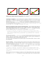
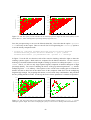
Figure 4.3: Comparison of the finished multi-chromosomal S. cerevisiae (x-axis) and the draft genome S.
paradoxus (y-axis). Red lines are chains between strands with the same orientation and green lines are chains
between strands with different orientations (inversion).
The arguments -v, -plot, -align, are as defined before in Sections 4.1, i.e, -v for verbose mode,
-plot for producing 2D postscript plot, and -align for producing alignment on the character level.
The parameters estimated (e.g., minimum fragment length, and maximum gap between fragments) for
comparing these three genomes are stored in the automatically generated file parameters.auto.
You can re-edit the paramters and pass this file to CoCoNUT and run the system again, starting from
the phase with the changed paramters using the options usematch, usechain, or usealign. For
more details about the format of the parameter file, see Section 6.2. The other options are handled in
the tutorial of Chapter 6.
4.2.4 Output files
We have the same types of output files as mentioned in the previous Section. In addition, we have
the extra *.ctg files which report coordinates relative to the contig/chromosome along with the
contig/chromosome number, and we have some more intermediate files needed for completing the
processing pipeline.
To visualize the output chain with respect to the first and second genome, run
> gv testdata/draft/yeast/fragment.mm.ccn.1x2.gp.ps
The resulting chains are plotted in the file testdata/draft/yeast/fragment.mm.ccn.1x2.gp.ps;
see Figure 4.3 (left).
To visualize the output syntenic regions with respect to the first and second genome, run
> gv testdata/draft/yeast/fragment.mm.ccn.dat.syn.1x2.ps
Figure 4.3 (right) shows the postscript files for the resulting regions.
Below is a snapshot of the alignment file testdata/draft/yeast/fragment.mm.pp.chn.align,
where we show its header and part of the first chain. (Dots in the alignment refers to matching character with that of the first sequence.) Details of the alignment file format is given in Section 5.5. For the
25
alignment output, the user can choose to report coordinates either w.r.t. the concatenated sequences or
w.r.t. each contig/chromosome.
#
#
#
#
#
#
Number of genomes: 2
Seq 1: testdata/draft/yeast/yeast_genome
Seq 2: testdata/draft/yeast/s.paradoxus.scfld
Chain file: testdata/draft/yeast/fragment.mm.pp.chn.ordered
Orientation: + +
Chain display options: palindrome, absolute positions
# Chain no. 1
# Contigs 1 1
# Boundaries: 538:1677-2214 530:2824130-2824659
28:1677-1704 28:2824130-2824157
97:1705-1801 88:2824158-2824245
Seq 1:TACGGTATTTATATCATCAAAAAAAAGTAGTTTTTTTATTTTATTTTGTTCGTTAATTTT 60
Seq 2:A..T..._...................C........._.....__.._.._........C
Seq 1:CAATTTCTATGGAAACCCGTTCGTAAAATTGGCGTTT
Seq 2:....G.......G.TTT.A....._...__.....CC
46:1802-1847 46:2824246-2824291
1:1848-1848 1:2824292-2824292
Seq 1:G
Seq 2:A
35:1849-1883 35:2824293-2824327
28:1884-1911 28:2824328-2824355
Seq 1:AACACCGGTGATCATTCTGGTCACTTGG
Seq 2:T....................G.....A
If you could visualize the files and read the alignment file, then your installation for this task is
successful.
4.3 Repeat analysis
.
4.3.1 Test data
Our test data is the Arabidopsis chromosome I. The sequence file is called chr1.fasta in the test
data distributed with CoCoNUT), and we assume it resides in the directory testdata/repeat/Arabidposis
within the CoCoNUT directory.
4.3.2 Main options of CoCoNUT
To see the main options of this task, run the following command.
> coconut.pl -repeat
26
Usage: frepeats.pl
Options:
-pr
-v
-forward
-align
-plot
-plotali X
-indexname
-useindex
-usematch
-usechain
-usealign
-prefix
-sysntenic
:
:
:
:
:
:
:
:
:
:
:
:
:
<Options> input_seq
parameter file (optional), if not given defaults are computed
verbose mode, i.e., deisplay of the program steps
run the comparison for forward strands only
compute alignment
produce Postscript 2D plots of the chains
filter out alignments with idenetity < X (0< X <= 1) and produce 2D plots
specify the index if constructed
do not construct index again
do not compute matches again, this construct no index
use the computed chains and complete processing
use the computed alignments and complete processing
specify a prefix name for the output files
computes sysntenic regions by removing repeats and applying
1D chaining over all dimensions.
4.3.3 Calling CoCoNUT
CoCoNUT is called as follows:
> coconut.pl -repeat testdata/repeat/Arabidposis/chr1.fasta -v \
-plot -align -syntenic
The arguments -v, -plot, -align, are as defined before in Sections 4.1, i.e, -v for verbose mode,
-plot for producing 2D postscript plot, and -align for producing alignment on the character level.
The parameters estimated (e.g., minimum fragment length, and maximum gap between fragments) for
comparing these three genomes are stored in the automatically generated file parameters.auto.
You can re-edit the paramters and pass this file to CoCoNUT and run the system again, starting from
the phase with the changed paramters using the options usematch, usechain, or usealign. For
more details about the format of the parameter file, see Section 7.2. The other options are handled in
the tutorial of Chapter 7.
4.3.4 Output files
We have the same types of output files as in Section 4.1. This is because finding repeated regions can
be regarded as comparing the sequence to itself.
To visualize the resulting 2D plot, run
> gv testdata/repeat/Arabidposis/fragment.mm.ccn.1x2.gp.ps
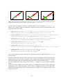
The resulting chains are plotted in the file testdata/repeat/Arabidposis/fragment.mm.ccn.1x2.gp.ps;
see Figure 4.4 (right).
To visualize the output syntenic regions, run
> gv testdata/repeat/Arabidposis/fragment.mm.ccn.dat.syn.1x2.ps
Note that the reported are repeats with just one copy. Repeats with more than one copy are filtered
out.
27
3.5e+07
3e+07
3e+07
testdata/repeat/Arabidposis/chr1.fasta
testdata/repeat/Arabidposis/chr1.fasta
3.5e+07
2.5e+07
2e+07
1.5e+07
1e+07
5e+06
2.5e+07
2e+07
1.5e+07
1e+07
5e+06
0
0
0
5e+06
1e+07
1.5e+07
2e+07
2.5e+07
testdata/repeat/Arabidposis/chr1.fasta
3e+07
3.5e+07
0
5e+06
1e+07
1.5e+07
2e+07
2.5e+07
testdata/repeat/Arabidposis/chr1.fasta
3e+07
3.5e+07
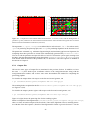
Figure 4.4: The chains corresponding to the repeated regions in the Arabidopsis chromosome 1. The x- and y- axis are
for the same chromosome. Note that the area above the upper diagonal is the one containing chains. The other area is not
plotted because it is symmetric to the first one.
Figure 4.4 (left) shows the postscript files for the resulting regions. The large genomic regions are now
much more clearer on the upper-right corner of the plot. Note that a more refined strategy including a
second chaining step is handled in Chapter 7.
The alignment file looks like the one in Section 4.2. If you could visualize the files and read the
alignment file, then your installation for this task is successful.
4.4 cDNA mapping
4.4.1 Test data
We use the A. thaliana chromosome 1 and a database of A. thaliana cDNAs. These example sequences
are distributed with CoCoNUT test data, and we assume they reside in the directory testdata/cdna/Arabidposi
under the names chrom1.seq and cdna.seq, respectively.
4.4.2 Main options of CoCoNUT
To see the main options of this task, run the following command.
> coconut.pl -map
Usage: perl coconut.pl
Options:
-pr
-v
-forward
-align
-plot
-plotali X
-indexname
-useindex
-usematch
-usechain
-usealign
:
:
:
:
:
:
:
:
:
:
:
<Options> -cdna cdna_database -gdna genome_seq
parameter file (optional), if not given defaults are computed
verbose mode, i.e., deisplay of the program steps
run the comparison for forward strands only
compute alignment using clustalw
produce Postscript 2D plots of the chains
filter out alignments with idenetity < X (0< X <= 1) and produce 2D plots
specify the index if constructed
do not construct index again
do not compute matches again, this construct no index
use the computed chains and complete processing
use the computed alignments and complete processing
28
-prefix
: specify a prefix name for the output files
-o [chainer|
blast] : specify output format (chainer|blast), chainer format is default
-cluster
: Find cluster of genes mapped to the same locus, and report
repeated genes
4.4.3 Calling CoCoNUT
> coconut.pl -map -cdna testdata/cdna/Arabidposis/cdna1.seq -gdna
testdata/cdna/Arabidposis/chrom1.seq -v -plot -align -o blast
The parameters estimated (e.g., minimum fragment length, and maximum gap between fragments) for
comparing these three genomes are stored in the automatically generated file parameters.auto.
You can re-edit the paramters and pass this file to CoCoNUT and run the system again, starting from
the phase with the changed paramters using the options usematch, usechain, or usealign. For
more details about the format of the parameter file, see Section 8.2. The other options are handled in
the tutorial of Chapter 8.
4.4.4 Output files
We basically have the same files as described in Section 4.1. Note that some files have not yet been
produced, because the respective options are not set. For example, a cluster file, which clusters the
cDNAs mapped to the same genome location, is not produced; see Chapter 8 for more details.
To visualize the resulting 2D plot, run
> gv testdata/cdna/Arabidposis/fragment.mm.ccn.1x2.gp.ps
The resulting chains are plotted in the file testdata/repeat/Arabidposis/fragment.mm.ccn.1x2.gp.ps;
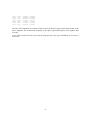
see Figure 4.5.
Here is a snapshot of the resulting alignment file (including the header) in BLAST format. Dots in
the alignment refers to matching character with that of the first sequence. For each exon, we write the
starting and end positions in the respective cDNA and in the genomic sequence.
# Chain file : testdata/cdna/Arabidposis/fragment.mm.pp.chn.ctg.ordered
# Genome file: testdata/cdna/Arabidposis/chrom1.seq
# cDNA file : testdata/cdna/Arabidposis/cdna1.seq
#**************
# Chain no.: 1
# AT1G08520.1, id: 1
# cDNA length: 2548
# Identity: 2548 = 100%
Exon 0:
cDNA:0-398, gDNA:2696414-2696812
GCAATCAGGAAAGGATGACGAGACAAAAGATAGAGAAGCAAAAGTAAGCTGATAAGGTTT 59
............................................................ 2696473
GATACAGTAGAAAATACTATCTCTTAACTTCTTCTTCTTCTTCTTCTTCTTCTCCTATCT 119
............................................................ 2696533
29
3.5e+07
3e+07
testdata/cdna/cdna1.seq
2.5e+07
2e+07
1.5e+07
1e+07
5e+06
0
0
2e+06
4e+06
6e+06
8e+06
1e+07
1.2e+07
1.4e+07
testdata/cdna/chrom1.seq
Figure 4.5: The plot of the mapped Arabidopsis cDNAs (x-axis), and the first Arabidopsis genome (y-axis). Left: The
mapped chains. The range of the x-axis is the whole cDNA length, and the position of a cDNA is its position w.r.t. the
whole database, i.e., w.r.t. the concatenated cDNA sequences.
TTGAAAATGGCGATGACTCCGGTCGCGTCATCATCTCCAGTTTCAACCTGCAGACTCTTT 179
............................................................ 2696593
CGCTGCAATCTCCTCCCTGATCTCTTACCTAAGCCTCTGTTTCTCTCCCTCCCCAAACGA 239
............................................................ 2696653
AACAGAATTGCCTCGTGCCGCTTCACTGTACGTGCCTCCGCGAATGCTACCGTCGAATCC 299
............................................................ 2696713
CCTAACGGTGTCCCTGCCTCCACATCAGATACGGATACGGAGACGGATACCACCTCCTAT 359
............................................................ 2696773
GGCCGACAGTTTTTCCCTTTGGCCGCAGTTGTTGGCCAG
.......................................
Here is a snapshot of the alignment file (including the header) in the chainer format.
# Chain file : testdata/cdna/Arabidposis/fragment.mm.pp.chn.ctg.ordered
# Genome file: testdata/cdna/Arabidposis/chrom1.seq
# cDNA file : testdata/cdna/Arabidposis/cdna1.seq
#**************
# Chain no.: 1
# AT1G08520.1, id: 1
# cDNA length: 2548
# Identity: 2548 = 100%
[0, 398] [2696414, 2696812]
[399, 577] [2697017, 2697195]
[578, 662] [2697285, 2697369]
[663, 979] [2697455, 2697771]
[980, 1103] [2697874, 2697997]
[1104, 1196] [2698113, 2698205]
[1197, 1292] [2698629, 2698724]
[1293, 1436] [2698973, 2699116]
30
[1437,
[1644,
[1800,
[1908,
[2043,
[2202,
[2323,
1643]
1799]
1907]
2042]
2201]
2322]
2547]
[2699196,
[2699469,
[2699815,
[2700023,
[2700257,
[2700520,
[2700736,
2699402]
2699624]
2699922]
2700157]
2700415]
2700640]
2700960]
The tail of the alignment file contains statistics about the donor/acceptor profil matrix based on the
splice alignment, the di-nucleotide frequency at the splice sight and histogram of the aligned chain
coverage.
If you could visualize the files and read the alignment file, then your installation for this task is
successful.
31
Chapter 5
Comparison of finished genomes
In this chapter, we discuss the comparison of finished genomes. For single-chromosomal genomes,
each genome must be given as a single fasta file. Multi-chromosomal genomes should be compared
by all pairwise comparison of chromosomes, where each chromosome is given as a single fasta file.
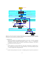
Figure 5.1 summarizes the task of comparing multiple genomes in the CoCoNUT system. The input
to the system is a set of genomic sequences. The basic steps done in any comparison are fragment
generation and chaining. After running these two phases the user can finish the comparison or proceed
to (1) visualize the resulting chains by producing 2D plots, (2) perform an alignment on the character
level for each chain, (3) compute syntenic regions, or (4) perform a second chaining step over the
produced chains. Then use these results to compute again the syntenic regions and plot the chains.
After computing the alignment, the regions of low sequence identity are filtered out. Then it is possible
to detect the syntenic regions or perform a second chaining step.
For repeating some parts of the comparison with different parameters, the user can re-start the comparison at four points: (1) after the index generation, (2) after the fragment generation, (3) after the
first chaining, and (4) after finishing the alignment. For example, if the user already computed the
fragments, and computed the chains, then he could run the alignment program later using the already
computed fragments and chains. He can also repeat this step with different parameters.
5.1 Calling CoCoNUT
The program CoCoNUT is called as follows:
> coconut.pl -multiple -fp multimat|ramaco [options] genome1 . . . genomek
Here is a description of the options:
-multiple
Specifies the task of comparing two or more finished genomes.
-fp multimat|ramaco
The user must specify whether the program multimat or ramaco is used for generating the
fragments.
32
> gi genome 1
GCCGCGCGT
CGGT
CG..
Input genomes
Fragment Generation Phase
Construct Index
use index & proceed
(.p[p|m]+) Compute Fragments
use fragments & proceed
Chaining Phase
(.chn, .ccn, .stc)
Chaining
use chains & proceed
Post−processing Phase
(.ps)
Synteny & Repeat filter
Alignment
2D Plots
(.syn)
(.align)
2D Plots
Filter alignment with
identity < T
(.align.filtered, .chn.filtered,
.ccn.filtered, .stc)
2D Plots
(.syn*.ps)
use alignment & proceed
Synteny & Repeat filter
(.filtered.syn)
(.filtered*.ps)
2D Plots
(.filtered.syn*.ps)
Recursive Chaining
Chaining
2D Plots
Synteny & Repeat filter
2D Plots
Figure 5.1: A flow chart for the task of comparing multiple genomes. The user can repeat the comparison starting from
the four points use index, use fragment, use alignment, and use chain and proceed further in the comparison. The brackets
beside each box enclose the file extensions produced by each step.
-pr parameter
file
Specifies the parameter file containing the parameters of the system. This file is generated
automatically, if no file is specified. All the options, except for -v and -plot, are functionless
if a parameter is specified. That is, the options in the parameter file dominate. The format of
the parameter file is given in Section 5.2.
-forward
run the comparison for forward strands only. This option is functionless if a parameter file is
given. Restricting the processing to the forward strand only is achieved by deleting the option
-p from the fragment line in the parameter file.
-plot
produce Postscript 2D plots of the chains. For multiple genomes, the plots are projections of
33
the chains w.r.t. each pair of genomes.
-align
compute an alignment on the character level for the homologous regions.
value 0 < τ ≤ 1
filter out alignments with percentage identity < τ and produce 2D plots.
-plotali filter
-syntenic
compute syntenic regions. This option is based on a program called chainer2permutation.x,
which first removes repeats and applying 1D chaining over all dimensions. As default, regions
overlapping with at least 70% of their length are filtered out as repeats. Moreover, it is allowed
that a fragment can overlap with the successive one in a 1D chain with at most 20% of its
length.
-useindex
do not construct the index again. This option is useful if one repeats the comparison with
different fragment parameters. Also, with the program ramaco, one can compare the indexed
genome to another genomes without re-constructing the index.
-indexname
specify the index, if constructed. This option is useful to use indices that are already constructed,
and stored somewhere in your system.
-usematch
do not compute the fragments again. With this option the constructed index is used again.
-usechain
use the computed chains and proceed in processing.
-usealign
use the computed alignments and proceed in processing.
-prefix prefix
name
specify a prefix name for the output files. This prefix name should include the destination path,
otherwise the resulting files will be in the CoCoNUT directory. If this option is not set, then the
default prefix for the index is Index and for the fragments and post-processing is fragment.
The resulting files will be stored in the directory in which the first input genome resides.
-v
verbose mode, i.e., display of the program steps.
5.2 The parameter file
The parameter file contains parameters for each step in the comparison. The parameter file, if not
specified, is automatically generated with parameters estimated statistically. Below is an example of
a parameter file for the program multimat. The lines separated by # are comment lines. The line
starting with “FRAGMENT=” specifies the parameters passed to the fragment generation programs
multimat/ramaco. The line starting “CHAINING=” specifies the parameters passed to the chaining
program CHAINER. The lines starting with “ALIGN=” specifies parameters passed to the program
34
alichainer used to generate the alignment. Finally the line “SYNTENY=” specifies the parameters
passed to the program chainer2permutation.x that determines syntenic regions and reports permutations. In the remaining part of this chapter, we handle each of these parameters in detail along with
the respective program implementing it.
FRAGMENT= -p -d -v -l 20
CHAINING= -l -chainerformat -lw 7 -gc 100 -length 40
ALIGN= -palindrome
SYNTENY= -overlap1 0.2 -filterrep 0.7
5.3 The fragment generation phase
There are two fragment generation programs that can be used when comparing multiple finished
genomes: multimat and ramaco. While multimat is based on an index constructed for all the sequences, ramaco constructs the index for the first sequence and takes the other sequences as queries.
(In CoCoNUT, we assume that the user inputs the shortest sequence first.) The rareness value must be
set in ramaco, but it is optional to do so in multimat.
In the parameter file, the line starting with “FRAGMENT=” specifies the parameters passed to the
multimat/ramaco program. The parameters for multimat are
-l ℓ
to specify the minimum fragment length, i.e., generate fragments with length at least ℓ,
-d
to generate fragments for the positive strands only,
-p
to generate fragments between all the positive and negative strands. If there are multiple
genomes, then fragments from all combinations between the positive and negative strands are
computed. For example, let “p” and “m” denote a positive and a negative strand, respectively. For three genomes, we have fragments from the combinations “ppp”, “ppm”, “pmp”,
and “pmm”.
-v
verbose mode, where some more details are stored in the output match file.
To restrict the processing to the forward strand only, one should delete the option -p from the fragment
line.
Another important parameter for multimat is the option “-unitol r”. This option generates multiMEMs such that the substrings comprising the match appear at most r+1 times in one of the sequences
(of course the substring appears at least once in each sequence). With r = 0, the reported matches are
multi-MUMs. For two sequences, these are the well-known MUMs.
For ramaco, we write just the minimum fragment length and the rareness value, which is equivalent to
-unitol. The following is an example showing how to write the fragment parameters when using
the program ramaco.
35
FRAGMENT= 20 5
CHAINING= -l -chainerformat -lw 27 -gc 500 -length 40
For the automatically generated parameter file, the “-unitol” option and the rareness value is set to
five.
5.3.1 The fragment generation parameters
Now, we discuss some issues about setting the parameters of the fragment generation phase.
The minimum fragment length The default minimum fragment length is estimated using a statistical model, which is suitable in average for all comparisons. However, for closely related sequences, the minimum fragment length can be increased, to avoid generating redundant fragments
and unnecessarily increase the comparison time. For distantly related sequences, the minimum fragment length should be decreased as much as possible to achieve high sensitivity. Thus, we suggest you first run the system with the default parameters, unless you know that the sequences are
closely related. Then you can reduce the minimum fragment length in the generated parameter
file, which is called parameters.auto. Afterwards, you run the system again using the option
“-pr parameters.auto”, which sets the parameter file option. This procedure can be repeated
until no improvement is observed.
The rareness value: On the one hand, using the rareness options makes it possible to assign the
minimum fragment length parameter a value less than the one set without the rareness value, which
is useful when detecting syntenic regions of highly divergent, but less repetitive, genomes. On the
other hand, setting these options should be done with some care. This is because homologous regions
repeated more than r times will not be detected.
5.3.2 The choice of the fragment generation program
To conclude this issue, Figure 5.2 shows a flowchart to help the user to make a decision whether
multimat or ramaco should be used. The program ramaco is basically designed for rare-multi-MEMs,
and it has two interesting features:
1. The index is constructed for only one sequence, and the other sequences are sequentially
matched as queries against this index to compute the fragments. This feature enables one to
run large scale comparisons with minimal memory requirement. Moreover, the constructed
indices can be used later for comparison with other genomes, in connection with the option
-useindex of CoCoNUT.
2. The intermediate comparison results can be stored so that the fragment generation between a
new genome and already processed genomes can be done without repeating the whole experiment. For example, if we compare two genomes, say g1 and g2 , then the index is constructed
for g1 and some intermediate information will be stored when querying g2 . If a third genome
is to be compared to g1 and g2 , then the intermediate information can be used to generate the
fragments between the three genomes. I.e., we save constructing the index of g1 and querying
36
yes
yes
memspe
rareness value
for each seq. ?
yes
rareness value?
no
no
memory limit?
memspe
no
multimat
multimat
Figure 5.2: A flow chart to decide if to use multimat or ramaco.
g2 again. This feature is not implemented in CoCoNUT, but the user can make use of it (by
editing some external script) and then use CoCoNUT to further process the resulting fragments;
see the manual of ramaco for more details about this feature.
5.4 The chaining parameters, and the program CHAINER
The chaining step in the CoCoNUT system is performed using the program CHAINER. In this chapter
we discuss the parameters related to the comparison of multiple genomic sequences. In the above
example of the parameter file, the line starting with “CHAINING=” specifies the parameters passed
to this program. These parameters are
-l local
chaining
to solve the local chaining program. The gap cost between the fragments in a local chain is the
L1 distance between the start and end points of the fragments.
-chainerformat
to report the resulting chains in CHAINER format. The resulting chain files have extension
“.chn”. For chains computed w.r.t. the reverse complement of any sequence, the coordinates are
given w.r.t. the reverse complement sequences. CHAINER can report output in another tablewise format with extension *.dbf. However, in the CoCoNUT system we use the CHAINER
format for the following phases of the system. In other words, if it is required to produce only
chains without visualization and post-processing, one can use the default format or report to
the stdout with the option “-stdout”; see the CHAINER manual for more details about the other
formats.
-gc gap
constraint
specifies the maximum gap length allowed between two fragments in the chain. For example,
-gc 300 imposes that the start and end point of two fragments fi and fi+1 in a local chain are
not separated by a distance larger than 300 bp in any genome, i.e., beg(fi+1 ).xr − end(fi ).xr ≤
300 for every genome 0 < r ≤ k.
-lw multiplying
factor
multiplies the weight of every fragment by a numerical value ℓ and uses the result as the weight
37
of the fragment. The value ℓ can be a non-integer value. The default value for ℓ is 1 for global
chains without gap costs and for cDNA/EST mapping, while it is 10 otherwise. Using this
option is essential for finding homologous regions of reduced sequence conservation. In other
words, to connect fragments with larger gap distances.
-length average
chain length
specifies the minimum average chain length. For k genomes and a chain starting with fragment
f and ending with fragment f ′ , the average chain length is
k
1X
(end(f ′ ).xi − start(f ).xi )
k
i=1
For example, -length 50 yields all representative local chains whose average length is larger
than or equal to 50.
Other options of CHAINER that can be used with option “-l” include the following:
-s score
Specify the minimum score of the reported chains; the default value is zero. For example, -s
500 yields all representative local chains whose score is larger than or equal to 500.
-perc percentage
reports chains whose minimum score is higher than a percentage of the highest score of a local
chain. For example, -perc 80 reports all chains whose score is at least 80% of the highest
score of a local chain. Note that we take the maximum of the two parameters -perc and -s if
both are set to different values.
-d chain
size
specifies the chain size, i.e., the minimum number of fragments in a reported chain.
-cluster cluster
file
reports cluster of chains in a cluster file; see CHAINER manual for details.
-stdout standard
output
Output the chains to the standard output. The chains are reported in table format; see the
CHAINER manual for more details. The default output in CHAINER is to store the chains in
table-format in a file with extension .dbf. But for CoCoNUT, we adopt the CHAINER format.
See the CHAINER manual (distibuted with CoCoNUT manual) for more details about these and other
options.
5.4.1 The input and output files for the chaining step
The fragment file produced by the fragment generation program is first transformed to the CHAINER
format. Below is an example of a fragment file for three genomes in CHAINER format. The first
line is a header line containing the keyword >CHA 3 and specifying the number of genomes. Each
fragment starts with the character #, which is followed by the fragment weight. As default in our
system, the fragment weight is its length. The ith bracket encloses the start and end positions of the
fragment in the ith genome. For example, the first fragment in this file starts at position 225137 and
ends at position 225150 in the second genome.
38
>CHA 3
#14
[938654,938667] [225137,225150] [214465,214478]
#14
[862792,862805] [437801,437814] [138894,138907]
#14
[1041684,1041697] [949290,949303] [317847,317860]
The format transformation step includes also a classification of the fragments w.r.t. the DNA strand.
Let the set of strings p[m|p]k−1 of length k denote the combinations of all comparisons involving positive and negative strands for k genomes, where p and m stand for the positive and negative strands,
respectively. For example, if we have three genomes, then we have the strings ppp, ppm, pmp, pmm.
The string ppp stands for comparing the three positive strands of all the genomes, and the string pmp
corresponds to the comparison among the positive strand of the first genome, the negative strand of
the second genome, and the positive strand of the third genome. Assume the fragment file generated
by the fragment generation program is called fragment, then the resulting files after the transformation have the extensions p[m|p]k−1 . For three genomes, we have the files fragment.ppp,
fragment.ppm, fragment.pmp, and fragment.pmm.
In the transformation step, it is also assured for a fragment from some negative strands that the coordinates in the negative strands are given w.r.t. the negative strands. (Note that the coordinates output
from multimat and ramaco are w.r.t. the positive strand only.)
The chaining step is done for each of the files output from the transformation program separately.
That is, for the three genomes in the example given above, the chaining step is performed for each
one of the four files separately. The output of the chaining step includes, for each combination, the
following set of files:
• chain files with extension *.chn: These files contain the computed chains. For the three
genomes in the example given above, we have as output the files fragment.ppp.chn,
fragment.ppm.chn, fragment.pmp.chn, and fragment.pmm.chn. Below is an
example of a chain file for three genomes containing two chains:
>CHA 3
#4527.000000
[1018162,1018192]
[1018109,1018158]
#2172.000000
[1016423,1016436]
[1016318,1016331]
[1015908,1015927]
[1015863,1015880]
[1175914,1175944] [293565,293595] 1800
[1175861,1175910] [293512,293561] 2378
[1174342,1174355]
[1174237,1174250]
[1173827,1173846]
[1173782,1173799]
[291826,291839]
[291721,291734]
[291311,291330]
[291266,291283]
971
1871
2034
1744
The first line is a header line containing the keyword >CHA 3, specifying the number of
genomes. Each chain starts with the character #, which is followed by the chain score. The
fragments composing the chain are written in the following lines in a descending order. At the
end of the line defining the fragment, the fragment id. (number) in the fragment file is given.
• compact chain files with extension *.ccn: These files contain chain files but in a compact
form. That is, the chain boundaries are given without the fragments of each chain. For the
above chain file, the compact chain file is
39
>CHA 3
#4527.000000
[1018109,1018192] [1175861,1175944] [293512,293595]
#2172.000000
[1015863,1016436] [1173782,1174355] [291266,291839]
For the three genomes example given above, we have as output the files fragment.ppp.ccn,
fragment.ppm.ccn, fragment.pmp.ccn, and fragment.pmm.ccn.
• statistics files with extension *.stc: This file contains statistics about the chaining task. Here
is an example of a statistics file
3 3041 262 14
1041888 1229966 1069216
# no. of chains: 112
The numbers from left to right in the first line are number of genomes, number of fragments,
maximum fragment length, and minimum fragment length. The numbers in the second line
are the maximum end positions of the fragments in each genome. The third line stores the
number of computed chains. For the three genomes example given above, we have as output the files fragment.ppp.stc, fragment.ppm.stc, fragment.pmp.stc, and
fragment.pmm.stc.
5.4.2 The chaining parameters and the recursive chaining option
Now, we discuss two issues regarding the chaining step: The chaining parameters, and the recursive
chaining.
The chaining parameters
The most important parameters that affect the sensitivity and specificity of the procedure are (1) the
multiplying factor lw and (2) the gap constraint gc.
The multiplying factor should be adjusted in connection with the gap constraint, and the minimum
fragment length parameter. As we mentioned before, the score of a chain C is
score(C) =
t
X
fi .length −
ℓ−1
X
g(fi+1 , fi )
i=1
i=1
A significant chain should have score larger than zero. With the multiplication factor, the chain score
is
ℓ−1
t
X
X
g(fi+1 , fi ) > 0
lw × fi .length −
score(C) =
i=1
i=1
Assume, in the worst case, that a chain has only two fragments f1 and f2P
and assume that both
fragments has the minimum fragment length ℓ. For the L1 metric, g(f1 , f2 ) = ki=1 (f2 .xi −f1 .xi ) =
k × gc, and we have
2 × lw × ℓ − k × gc > 0
40
For automatically generated files, we set gc = 500 for two genomes, and gc = 1000 for more than
two genomes. We then use the above formula to compute lw .
Note that this is the worst case for a chain in our program, because a similar region usually has a chain
of multiple fragments.
Recursive chaining
In CoCoNUT, we can call CHAINER iteratively to chain the produced chains, or to chain the filtered
chains. In other words, the user can directly carry out a second chaining step over the resulting chains,
or he can first compute detailed alignment over the chains on the character level then carry out a
second chaining. . The option -plotali τ should be set to filter out chains whose alignment has
percentage identity < τ . The first chaining step is basically to find locally aligned regions. The
second chaining step can be used to help identifying syntenic regions automatically. To have a second
chaining step, one should edit a second chaining command in the chain file. CHAINER has a special
option for this task called -neighbor. This option requires just to specify the gap constraint, since
the multiplying factor is forced to be lw = 1, and the gap cost function g(f, f ′ ) is the constant function
zero. That is, this option works as if we cluster the fragments based on their neighborhood. The choice
of the gap constraint parameter with the option -neighbor is up to the user, and it is actually very
dependent on the evolutionary distance between the genomes. According to our experiments, we
observed that for closely related bacteria, the number lies in the range 10 to 50 Kbp. For a comparison
of the human genome with the mouse genome, it is between 1 to 2 Mbp. That is, we recommend that
the user runs this step with different parameters. Note that the user can use the options -usechain
to just perform this step without repeating the steps of the comparison from the beginning, i.e., the
previously computed index, fragments, and chains of the first step are used. At the end of this chapter,
we shed more light on this option.
The user should not confuse this option with the syntenic option, discussed later. The recursive chaining step is basically used to find larger chains. When these chains are input to the syntenic steps, small
re-arrangements lying within these large chains will be ignored, which is useful for studying genome
rearrangement on the macro-level. Note also that this option is not always needed for computing synteny. In most of the cases, it is enough to find the syntenic regions just after computing the chains,
removing low score ones, and filtering out the repeats.
5.5 The alignment parameters, and the program alichainer
In the parameter file, the line starting with “ALIGN=” contains the parameters passed to the program
alichainer used to compute alignments on the character level.
The options of alichainer that can be changed in the parameter file are as follows.
gap length
specifies maximal length of a region between the fragments of a chain to be aligned, default is
1000 bp. Regions longer than the given value will not be aligned. Note that this option should
be set in accordance with the gap constraint parameter of the chaining step. This fact can be
easily overlooked if the parameter file is manually re-edited.
-gl alignable
41
-palindrome
reports coordinates w.r.t. the forward strand, not w.r.t. the reverse complement one.
-match
show the nucleotide sequence of the aligned multi-MEMs.
-o mga|lineal
choose either mga/lineal output format. The MGA format is a BLAST like format introduced
first in the program MGA [6], in which the aligned regions are given in fasta format, or BLAST
like format; specifically the alignment is given in multiple lines, each is at most 60 characters
long. In the lineal mode, the alignment is given by a single line. The lineal mode is easier to
parse and can has use for visualization tools.
For this program, there are some additional output options specific to the alignment of draft genomes;
these will be discussed in Chapter 6.
The alignments are computed for each chain file, i.e., for each combination. For the three genomes
in the example given above, the input is the files fragment.ppp.chn, fragment.ppm.chn,
fragment.pmp.chn, and fragment.pmm.chn. The output of the files has the additional extension .align. For these files, the output is the following four files: fragment.ppp.chn.align,
fragment.ppm.chn.align, fragment.pmp.chn.align, and fragment.pmm.chn.align.
In Figure 5.3, we show a part of an alignment file fragment.pmp.chn.align. This file was
generated for the chain file fragment.pmp.chn. The first seven lines compose a header showing
the number of genomes, the genome names, the input chain file, the strand orientation, and the chain
display options.
The alignment of the ith chain starts with the line # Chain no. i. The next line # Contigs
1 1 1 is meaningful only when comparing draft genomes, here it has no significance, since the
genomes are finished (i.e., each genome is a single sequence). The third line specifies the chain length
and boundaries in each genome. In this example, # Chain no. i spans 233 bp in the first genome
from 51272 to 51504. In the second genome, whose negative strand is compared, the chain spans 230
from 432381 to 432610. The coordinates are given with respect to the positive strand of the second
genome, because the chain display option -palindrome was set.
Each fragment of the chain is given in a single line. This chain is composed of three fragments, these
are pointed to by arrows. The first fragment, e.g., has length 14 and starts at position 51272 and ends
at position 51285 in the first genome.
The regions between the fragments are given in the same format as the fragments but the alignment
of these regions follows directly the coordinate line. Each line in the alignment starts by the keyword
Seq i:, where i is the sequence number. The alignment line is limited to 60 characters. The points
in the alignment line corresponds to a character identical to the character of the first sequence that lies
in the same column.
After the last fragment of the chain, we report some statistics:
• Number of unaligned gaps: counts the number of unaligned gaps. Note that the length
of each un-aligned gap is higher than what is specified by the option -gl. In this example, no
such gaps exist.
42
#
#
#
#
#
#
#
Number of genomes: 3
Seq 1: testdata/chlamd/AE001273.fasta
Seq 2: testdata/chlamd/AE001363.fasta
Seq 3: testdata/chlamd/AE002160.fasta
Chain file: testdata/chlamd/fragment.mm.pmp.chn.ordered
Orientation: + - +
Chain display options: palindrome, absolute positions
# Chain no. 1
# Contigs 1 1 1
# Boundaries: 233:51272-51504 230:432381-432610 234:369584-369817
14:51272-51285 14:432597-432610 14:369584-369597
Fragment
145:51286-51430 145:432452-432596 146:369598-369743
Seq 1:gttgccttaccccaaatatgcaacaggatttggtgtgcgttgtttaattcattatatgga
Seq 2:agac.g...t..a........tt....t........t....c.a.tc..t....ct.a..
Seq 3:.c.t.....t..t.......................t............t........a.
Seq 1:gaaattcctatctaaatagttatt____gtttagcgatattaaa_taattgtgtgtggtt
Seq 2:a..tagt..t.....g.....gc.ttcta....ttt..g..tt.g....gact.t.at..
Seq 3:c..g..tt.............c..____......gtt.g.c...a...aaaga.t.....
60
120
Seq 1:agtttttaataaaaa_gttaaaaactaacca
Seq 2:tag....tt.....____.....gtc.tt__
Seq 3:g.........tttttta........c...._
17:51431-51447 17:432435-432451 17:369744-369760
Fragment
35:51448-51482 32:432403-432434 35:369761-369795
Seq 1:tcattctccctgtcgatagatcaaataagtagtag
Seq 2:ca..cg......c..........gg......a___
Seq 3:.......t......................g....
22:51483-51504 22:432381-432402 22:369796-369817
#
#
#
#
#
#
#
#
#
#
#
#
#
#
#
#
Fragment
Statistics:
Number of unaligned gaps: 0
Total Match length:
Seq: 1 :53
Seq: 2 :53
Seq: 3 :53
Total aligned gap length:
Seq: 1 :180
Seq: 2 :177
Seq: 3 :181
Total unaligned gap length:
Seq: 1 :0
Seq: 2 :0
Seq: 3 :0
Total identity in aligned gaps: 101
Percentage identity of chain: 0.660944 0.669565 0.658120
Figure 5.3: An example of an alignment file with one chain.
fragment.mm.pmp.chn file.
This file was generated from
• Total Match length: this counts the total exact fragment lengths. For the three fragments, we have totally 53 bp in each sequence.
• Total aligned gap length: this lists the total length of the regions between the frag-
43
ments in each genome. In this example, these are 180, 177, and 181 in the first, second, and
third genomes, respectively.
• Total unaligned gap length: this lists the total length of the unaligned gaps.
• Total identity in aligned gaps: this lists how many characters are identical in the
aligned gaps.
• Percentage identity of chain: this lists the ratio between the total identical characters (in fragments and in aligned gaps) and the chain length in each genome. In this example,
the percentage identities are ≈ 0.66, ≈ 0.67, and ≈ 0.66 in the first, second, and third genomes,
respectively.
5.6 The synteny parameters, and the program chainer2permutation.x
Two similar regions are considered syntenic, if (1) they appear in the same order in all given genomes,
and (2) they are not interrupted by any other segment.
The line “SYNTENY=” in the parameter file specifies the parameters passed to the program chainer2permutation.x,
which performs the following tasks over the computed chains, or the filtered chains (the alignment of
these chains has nucleotide identity larger than a user-defined threshold):
1. It filters repeated sequences.
2. It computes syntenic regions and reports permutations for these segments.
3. It plots the syntenic regions w.r.t. all pairwise projections.
A fragment is considered as a repeated one, if it is overlapping with another fragment with a factor τ
of its lengt, where τ is larger than a user-defined threshold.
We compute the syntenic regions by applying one-dimensional chaining iteratively w.r.t. each genome.
We allow that the fragments of the chain can overlap with a factor µ of its length, where µ is larger
than a user-defined threshold.
-overlap1 τ
The option -overlap1 τ permits any fragment in a chain to overlap with the next fragment
with percentage τ of its length.
-overlap2
This option allows any fragment in a chain to overlap with the next fragment with at most ℓ − 1
bp, where ℓ is the minimum region length.
-filterrep ration
The option -filterrep τ filters out any fragment overlapping with another fragment with
more than 100 × τ , 0 ≤ τ ≤ 1, of its length in any genome as a repeated one.
If no option is given, the default is not to filter repeats and allow no overlapping between the fragments
of the chain.
44
5.6.1 The input and output files
The input to the chainer2permutation.x program is a .dat file. This file contains the result of all
comparisons for all combinations in a gnuplot format. Below is an example of a .dat file. The
.dat file contains the fragment coordinates only w.r.t. the positive strand of all the sequences. There
is no score of each region. chainer2permutation.x takes the total length of the region in all genomes
as its score. Each region in a chain file is represented by two lines: The first line contains the point,
where the region starts in all genomes. The second line contains the point, where the region ends in
all genomes. Here is an example of a chain file. (The regions at the point zero are extra ones added to
ease the processing.)
#-- MATCHES pm
0
0
0
0
#-- MATCHES pp
0
0
0
0
1041677 317840
1041892 318058
1039820 316016
1040040 316236
The output files of chainer2permutation.x can be divided into the following groups:
• A synteny file with extension *.syn: An example of this file is given below. The first set
of lines are header lines containing the input *.dat file, the number of input regions, the
minimum region length in each genome, the total score in each 1D chaining step w.r.t. each
genome, and the final total score.
The following lines contain the permutations respective to the syntenic regions. These permutations are reported as follows. After filtering the repeats and computing the 1-dimensional
chains, they are sorted w.r.t. its order in each genome. Then we report the id of each region in
the input file (i.e., the region number in the input file). We then map the first permutation to the
identity permutation and rename the regions in the other genomes w.r.t. the identity permutation. The regions following each other with the same direction and not interrupted by any other
region are coalesced in a single compact region, which are then reported in a compact form.
For example, if genome one is composed of the three regions (+1 +2 +3), and the regions of
the second genome w.r.t. identity genome are (+1 -3 -2) and the regions of the third genome
are (+1 +2 +3), then the regions 2 and 3 can be coalesced, and the compact presentation of the
three genomes is (+1 +2), (+1 -2), and (+1 +2). In between, we report the synteny blocks in
non-compact form, and in compact form. (We use the word (non-) compact chain because of
the 1D chaining algorithm used.) The compact form, either for the blocks and the permutations,
is the final result of the synteny determination.
• A repeat file with extension *.rep.dat. The repeat file is given in .dat format.
• 2D plot files in postscript format with extension *.ps.
• Other intermediate files for producing the plots.
45
#
#
#
#
#
#
Input file: testdata/chlamd/fragment.mm.ccn.dat
Number of input regions = 406
Min. region length in sequences 1..k: 43 43
Total Score in dimension: 0 = 30298
Total Score in dimension: 1 = 29536
Total score: 59834
# Permutaions in terms of chain id’s in input file:
# Genome 1:
# Genome 2:
+1 +406 +405 +404 +403 .......
+1 +131 +130 +129 +128 .......
# Permutations w.r.t. identity permutation:
# Genome 1:
# Genome 2:
# Reporting
# + +
[0,0] [0,0]
# + +
[1564,3630]
# + +
[4211,4449]
# + +
[6999,7162]
...
...
...
+1 +2 +3 +4 +5 +6 +7 +8 +9 .....
+1 +277 +278 +279 +280 +282 ....
Optimal Non-compact Chain:
[320265,322331]
[322912,323150]
[325669,325832]
# Reporting Compact Chain:
# + +
[0,0] [0,0]
# + +
[1564,719983] [320265,1069389]
# + +
[720013,854021] [7,134526]
# + +
[854022,859132] [152153,157260]
# + +
[859977,873000] [136085,149033]
# + +
[880418,881177] [134544,135302]
# Compact permutations w.r.t. identity permutation:
# Genome 1:
# Genome 2:
+1 +2 +3 +4 +5 +6 +7
+1 +3 +6 +5 +4 +7 +2
5.7 The 2D plots
The 2D plots are generated for either (1) the chains, (2) the recursive chains, (3) the filtered chains
after the alignment, and (4) the syntenic regions. The option -plot generates plots for the chains
and recursive chains. Choosing the option -plot and -syntenic will automatically generate plots
for the filtered chains and the syntenic regions. In the 2D plots, each chains is represented by a line
connecting its start and end points in the genomes. Each 2D plot is a projection of the comparison
w.r.t. two genomes. For the three genomes example mentioned before and for plotting chains, we have
the three postscript files fragment.mm.ccn.1x2.gp.ps, fragment.mm.ccn.1x3.gp.ps,
46
5e+06
5e+06
5e+06
4.5e+06
4.5e+06
4.5e+06
3e+06
2.5e+06
2e+06
1.5e+06
4e+06
testdata/ecoli_shig/NC_007613.fasta
4e+06
testdata/ecoli_shig/NC_007613.fasta
testdata/ecoli_shig/NC_007384.fasta
4e+06
3.5e+06
3.5e+06
3e+06
2.5e+06
2e+06
1.5e+06
3.5e+06
3e+06
2.5e+06
2e+06
1.5e+06
1e+06
1e+06
1e+06
500000
500000
500000
0
0
0
500000
1e+06
1.5e+06 2e+06 2.5e+06 3e+06 3.5e+06
4e+06 4.5e+06 5e+06
0
0
500000
testdata/ecoli_shig/NC_000913.fasta
1e+06
1.5e+06 2e+06 2.5e+06 3e+06 3.5e+06
testdata/ecoli_shig/NC_000913.fasta
4e+06 4.5e+06 5e+06
0
500000
1e+06
1.5e+06 2e+06 2.5e+06 3e+06 3.5e+06
testdata/ecoli_shig/NC_007384.fasta
4e+06 4.5e+06 5e+06
Figure 5.4: Projections of the comparison of the three genomes E. sonnei, S. sonnei, and S. boydii. From left to right,
we have the projections 1x2, 1x3, and 2x3. Red lines correspond to chains between positive strands and green lines
correspond to chains between the +ve strand of the genome on the x-axis and the -ve strand of the genome on the y-axis.
and fragment.mm.ccn.2x3.gp.ps. The first file contains the projection of the chains w.r.t. the
first and second genomes, and the second contains the projection w.r.t. the first and third genomes,
and the third one contains the projection w.r.t. the second and third genomes. We use red lines in the
direction “north-east” to represent chains computed between forward strands, and use green lines in
the direction “south-east” to represent chains computed between the positive strand of the genome on
x − axis and the negative strand of the genome on y − axis. Figure 5.4 shows an example for 2D
plots from comparing three genomes.
For 2D plots of chains, the input to the plotting step are the compact chain files with extension *.ccn
computed by CHAINER. These files are processed to adjust the coordinates back to the positive strand,
and to transform the format into the gnuplot format.
5.8 Summary of output files
At this point, we summarize the resulting output files after carrying out each step. We recommend
to recall Figure 5.1 when reading this section. The following table describes the output files for each
step. Of course not all files are generated; only those that meet the users options. In this table, we
assume that the user assigns the resulting files the prefix fragment, which is also the fragment file
name.
47
Step
Fragment generation
Format transformation
First chaining
Alignment
Filtered Alignment
(filtered chains)
Second chaining
over compact chains
Second chaining
over alignment
(filtered chains)
Synteny
2D plots
files
fragment
fragment.p{p|m}+
Ex., fragment.pp, fragment.pm
1- Chain files with extension .chn
Ex., fragment.pp.chn, fragment.pm.chn
2- Compact chain files with extension .ccn
Ex., fragment.pp.ccn, fragment.pm.ccn
3- Statistics files with extension .stc
Ex., fragment.pp.stc, fragment.pm.stc
files with extension .align
Ex., fragment.pp.chn.align, fragment.pm.chn.align
The extension .filtered is added to the alignment, chain, and compact chain files
Ex., fragment.pp.chn.align.filtered,
fragment.pm.chn.align.filtered,
fragment.pp.chn.filtered,
fragment.pm.chn.filtered,
fragment.pp.ccn.filtered,
fragment.pm.ccn.filtered,
1- Chain files with extension .chn
Ex., fragment.pp.ccn.chn, fragment.pm.ccn.chn
2- Compact chain files with extension .ccn
Ex., fragment.pp.ccn.ccn, fragment.pm.ccn.ccn
3- Statistics files with extension .stc
Ex., fragment.pp.ccn.stc, fragment.pm.ccn.stc
1- Chain files with extension .chn
Ex., fragment.pp.ccn.filtered.chn, fragment.pm.ccn.filtered.chn
2- Compact chain files with extension .ccn
Ex., fragment.pp.ccn.filtered.ccn, fragment.pm.ccn.filtered.ccn
3- Statistics files with extension .stc
Ex., fragment.pp.ccn.filtered.stc, fragment.pm.ccn.filtered.stc
I. Files are generated with the extension .syn. For synteny over
1- first chaining, we have fragment.mm.ccn.syn
2- alignment, we have fragment.mm.ccn.filtered.syn
3- second chaining over chains, we have fragment.mm.ccn.ccn.syn
4- second chaining over alignment, we have fragment.mm.ccn.filtered.ccn.syn
II. Files are generated with the extension .rep.dat. For synteny over
1- first chaining, we have fragment.mm.ccn.dat.rep.dat
2- alignment, we have fragment.mm.ccn.filtered.dat.rep.dat
3- second chaining over chains, we have fragment.mm.ccn.ccn.dat.rep.dat
4- second chaining over align., we have fragment.mm.ccn.filtered.ccn.dat.rep.dat
The plots are with the extension .ps
1- For first chaining, we have fragment.mm.ccn.1x2.gp.ps
2- For alignment (filtered chains), we have fragment.mm.ccn.filtered.1x2.gp.ps
3- For second chaining over chains, we have
fragment.mm.ccn.ccn.1x2.gp.ps
4- For second chaining over alignment, we have
fragment.mm.ccn.filtered.ccn.1x2.gp.ps
5- For synteny over chains, we have
fragment.mm.ccn.dat.syn.1x2.ps
6- For synteny over alignments, we have
fragment.mm.ccn.filtered.1x2.gp.ps
7- For synteny over second chains over chains, we have
fragment.mm.ccn.ccn.dat.syn.1x2.ps
8- For synteny over second chains over alignments, we have
ffragment.mm.ccn.filtered.ccn.dat.syn.1x2.ps
5.9 Tutorial: Comparison of three genomes
To demonstrate the usage of CoCoNUT, we show step-by-step how to compare the three bacterial
genomes Escherichia coli, Shigella sonnei Ss046, and Shigella boydii Sb227. These genomes are in
the directory ∼/CoCoNUT/testdata/ecoli shig.
48
5e+06
5e+06
5e+06
4.5e+06
4.5e+06
4.5e+06
3e+06
2.5e+06
2e+06
1.5e+06
4e+06
testdata/ecoli_shig/NC_007613.fasta
4e+06
testdata/ecoli_shig/NC_007613.fasta
testdata/ecoli_shig/NC_007384.fasta
4e+06
3.5e+06
3.5e+06
3e+06
2.5e+06
2e+06
1.5e+06
3.5e+06
3e+06
2.5e+06
2e+06
1.5e+06
1e+06
1e+06
1e+06
500000
500000
500000
0
0
0
500000
1e+06
1.5e+06 2e+06 2.5e+06 3e+06 3.5e+06
4e+06 4.5e+06 5e+06
0
0
500000
testdata/ecoli_shig/NC_000913.fasta
1e+06
1.5e+06 2e+06 2.5e+06 3e+06 3.5e+06
4e+06 4.5e+06 5e+06
0
500000
testdata/ecoli_shig/NC_000913.fasta
1e+06
1.5e+06 2e+06 2.5e+06 3e+06 3.5e+06
testdata/ecoli_shig/NC_007384.fasta
4e+06 4.5e+06 5e+06
Figure 5.5: Projections of the comparison of the three bacterial genomes E. sonnei, S. sonnei, and S. boydii. From left to
right, we have the projections 1x2, 1x3, and 2x3.
Running with default parameters: From CoCoNUT basic directory, you can start the comparison
by using the default parameters. This is reasonable because it is assumed that we have no idea how
similar the three genomes are. We would like also to plot the chains, to see how good the parameters
are before computing the alignment. Therefore, we use the option -plot. Moreover, the verbose
mode option -v is used to see the intermediate step of the program. It would also be more convenient
to assign a prefix to the output files; we can choose the prefix EcSsSb. Because the genomes are of
small size, we can directly use the program multimat. The command line for calling CoCoNUT is
> coconut.pl -multiple -fp multimat testdata/ecoli_shig/NC_000913.fasta
testdata/ecoli_shig/NC_007384.fasta testdata/ecoli_shig/NC_007613.fasta
-v -plot -prefix testdata/ecoli_shig/EcSsSb
The following is the automatically generated parameter file, which is alway called parameters.auto
in our system. It sets the minimum fragment length to 15 bp and assigns 5 to the rareness value
-unitol. There is only one chaining step, where the length of each fragment is multiplied by 102.
The maximum gap between two fragments in a chain is set to 1000 bp. Chains with average length 30
bp are filtered out.
FRAGMENT= -p -d -v -unitol 5 -l 15
CHAINING= -l -chainerformat -lw 102 -gc 1000 -length 30
Now, we can have a look at the resulting plots. Let g1 , g2 , and g3 denote the three input genomes
given in the command line, respectively. Because we have three genomes, there are three projections: g1 × g2 , g1 × g3 ,, and g3 × g2 . These are stored in the files EcSsSb.ccn.1x2.gp.ps,
EcSsSb.ccn.1x3.gp.ps, EcSsSb.ccn.2x3.gp.ps. Figure 5.5 shows these plots.
In the same directory, the index files have prefix EcSsSb.index. The fragment file generated
by the program multimat is EcSsSb. The fragment files transformed to CHAINER format are
EcSsSb.pmm, EcSsSb.pmp, EcSsSb.ppm, and EcSsSb.ppp. The chain files are EcSsSb.pmm.chn,
EcSsSb.pmp.chn, EcSsSb.ppm.chn, and EcSsSb.ppp.chn. The compact chain files are
EcSsSb.pmm.ccn, EcSsSb.pmp.ccn, EcSsSb.ppm.ccn, and EcSsSb.ppp.ccn. The statistics files for the chains are EcSsSb.pmm.stc, EcSsSb.pmp.stc, EcSsSb.ppm.stc, and
EcSsSb.ppp.stc.
The coordinates in a chain file for a negative strand is given w.r.t. the negative strand. These coordinates are transformed back to the positive strand for plotting. The all compact chains for all
combinations are stored in the file EcSsSb.ccn.dat. From this file, the projections for producing
the plots are obtained.
49
5e+06
5e+06
5e+06
4.5e+06
4.5e+06
4.5e+06
3e+06
2.5e+06
2e+06
1.5e+06
4e+06
testdata/ecoli_shig/NC_007613.fasta
4e+06
testdata/ecoli_shig/NC_007613.fasta
testdata/ecoli_shig/NC_007384.fasta
4e+06
3.5e+06
3.5e+06
3e+06
2.5e+06
2e+06
1.5e+06
3.5e+06
3e+06
2.5e+06
2e+06
1.5e+06
1e+06
1e+06
1e+06
500000
500000
500000
0
0
0
500000
1e+06
1.5e+06 2e+06 2.5e+06 3e+06 3.5e+06
4e+06 4.5e+06 5e+06
0
0
500000
1e+06
testdata/ecoli_shig/NC_000913.fasta
1.5e+06 2e+06 2.5e+06 3e+06 3.5e+06
testdata/ecoli_shig/NC_000913.fasta
4e+06 4.5e+06 5e+06
0
500000
1e+06
1.5e+06 2e+06 2.5e+06 3e+06 3.5e+06
testdata/ecoli_shig/NC_007384.fasta
4e+06 4.5e+06 5e+06
Figure 5.6: The comparison of the three bacterial genomes E. sonnei, S. sonnei, and S. boydii, after filtering out chains
with average length less than 1000 bp. From left to right, we have the projections 1x2, 1x3, and 2x3.
Repeating some steps with better parameters: From the plots, we can directly observe that the
three genomes are highly similar. We can also conclude that the chains with smaller average length
might appear by chance. Therefore, we open the file parameters.auto and re-edit the option
-length 30 to be, say -length 1000. We then re-run CoCoNUT with the option -usematch
so that the steps of index construction and the fragment generation are not repeated again. (Note that
the changed option affects only the chaining step.) The command line is
> coconut.pl -multiple -fp multimat testdata/ecoli_shig/NC_000913.fasta
testdata/ecoli_shig/NC_007384.fasta testdata/ecoli_shig/NC_007613.fasta -v
-plot -prefix testdata/ecoli_shig/EcSsSb -pr parameters.auto -usematch
The resulting plots are shown in Figure 5.6.
Automatic detection of syntenic regions We might now want to have a look at how the synteny
based on the resulting chains look like. We open the file parameters.auto and add the line
SYNTENY= -overlap1 0.2 -filterrep 0.7. In order to re-use the previous comparison
results, we re-run CoCoNUT with the option -usechain.
coconut.pl -multiple -fp multimat testdata/ecoli_shig/NC_000913.fasta
testdata/ecoli_shig/NC_007384.fasta testdata/ecoli_shig/NC_007613.fasta -v
-plot -prefix testdata/ecoli_shig/EcSsSb -pr parameters.auto -usechain
The resulting plots are EcSsSb.ccn.dat.syn.1x2.ps, EcSsSb.ccn.dat.syn.1x3.ps,
and EcSsSb.ccn.dat.syn.2x3.ps These plots are shown in Figure 5.7.
Now we can have a look at the resulting reports for computing the synteny stored in the synteny file
EcSsSb.ccn.syn and repeat file EcSsSb.ccn.dat.rep.dat.
In the synteny file, we might have a look at the section reporting the compact permutations w.r.t. the
identity permutation. We can see that we have an identity permutation from 1 to 64. This means
that we have 63 synteny block (Number 1 in the permutation is just an imaginary reference one).
The content of this section can be passed further to a program for constructing phylogeny based on
rearrangement operations.
We can also scroll down in the file to the section for “Reporting Compact Chain:”. In this section, the
direction (w.r.t. positive and negative strands), and their coordinates (boundaries) w.r.t. the positive
strand is reported.
The repeat file EcSsSb.ccn.dat.rep.dat contains repeated chains in .dat file.
50
5e+06
5e+06
5e+06
4.5e+06
4.5e+06
4.5e+06
3e+06
2.5e+06
2e+06
1.5e+06
4e+06
testdata/ecoli_shig/NC_007613.fasta
4e+06
testdata/ecoli_shig/NC_007613.fasta
testdata/ecoli_shig/NC_007384.fasta
4e+06
3.5e+06
3.5e+06
3e+06
2.5e+06
2e+06
1.5e+06
3.5e+06
3e+06
2.5e+06
2e+06
1.5e+06
1e+06
1e+06
1e+06
500000
500000
500000
0
0
0
500000
1e+06
1.5e+06 2e+06 2.5e+06 3e+06 3.5e+06
testdata/ecoli_shig/NC_000913.fasta
4e+06 4.5e+06 5e+06
0
0
500000
1e+06
1.5e+06 2e+06 2.5e+06 3e+06 3.5e+06
testdata/ecoli_shig/NC_000913.fasta
4e+06 4.5e+06 5e+06
0
500000
1e+06
1.5e+06 2e+06 2.5e+06 3e+06 3.5e+06
testdata/ecoli_shig/NC_007384.fasta
4e+06 4.5e+06 5e+06
Figure 5.7: The comparison of the three bacterial genomes E. sonnei, S. sonnei, and S. boydii, after computing the synteny
over the chain files. From left to right, we have the projections 1x2, 1x3, and 2x3.
Computing the alignment: Now we might want to compute an alignment on the character level
for the chains. To compute the alignment, we have to edit the line ALIGN= -palindrome in the
parameter file parameters.auto. In order to re-use the previous comparison results, we re-run
CoCoNUT with the option -usechain. Use the same command line mentioned in the previous step.
The resulting alignment files are in the files: EcSsSb.pmm.chn.align, EcSsSb.ppm.chn.align
EcSsSb.pmp.chn.align, and EcSsSb.ppp.chn.align.
Filtering out alignments with low identity and plotting them: Now we might want to filter out
chains with percentage identity less than, say, 70%. To filter out alignments, and accordingly chains,
with percentage identity less than 70%, we use the option -plotali 0.7. In order to re-use the
previous comparison results, we re-run CoCoNUT with the option -usealignment.
> coconut.pl -multiple -fp multimat testdata/ecoli_shig/NC_000913.fasta
testdata/ecoli_shig/NC_007384.fasta testdata/ecoli_shig/NC_007613.fasta -v
-plot -prefix testdata/ecoli_shig/EcSsSb -pr parameters.auto -usealign
-plotali 0.7
By running the command ls -*filtered*, you can see all the produced files after this step of the
program. These files contain chains, compact chains, alignments, syntenic regions, and 2D plots of
the chains/alignment with percentage identity larger than 70%.
Let us have a look at the 2D plots of the syntenic regions over the filtered chains. Figure 5.8 shows
the resulting plots.
Recursive chaining: Recursive chaining can be performed over the chains or filtered chains whose
identity is larger than a user-defined threshold. To run the recursive chaining step over the produced filtered chains, add the line CHAINING= -neighbor -chainerformat -lw 1 -gc 50000
-length 1000 to the parameter file parameters.auto. Then we can call CoCoNUT again
using the -usealign option to re-use the already computed results.
> coconut.pl -multiple -fp multimat testdata/ecoli_shig/NC_000913.fasta
testdata/ecoli_shig/NC_007384.fasta testdata/ecoli_shig/NC_007613.fasta -v
-plot -prefix testdata/ecoli_shig/EcSsSb -pr parameters.auto -usealign
-plotali 0.7
For this option, the recursive chaining is carried out over the filtered chains because of the existence
of the option -plotali 0.7. This option forces any post-processing to run over the filtered chains.
51
5e+06
5e+06
5e+06
4.5e+06
4.5e+06
4.5e+06
3e+06
2.5e+06
2e+06
1.5e+06
4e+06
testdata/ecoli_shig/NC_007613.fasta
4e+06
testdata/ecoli_shig/NC_007613.fasta
testdata/ecoli_shig/NC_007384.fasta
4e+06
3.5e+06
3.5e+06
3e+06
2.5e+06
2e+06
1.5e+06
3.5e+06
3e+06
2.5e+06
2e+06
1.5e+06
1e+06
1e+06
1e+06
500000
500000
500000
0
0
0
500000
1e+06
1.5e+06 2e+06 2.5e+06 3e+06 3.5e+06
testdata/ecoli_shig/NC_000913.fasta
4e+06 4.5e+06 5e+06
0
0
500000
1e+06
1.5e+06 2e+06 2.5e+06 3e+06 3.5e+06
4e+06 4.5e+06 5e+06
0
500000
1e+06
testdata/ecoli_shig/NC_000913.fasta
1.5e+06 2e+06 2.5e+06 3e+06 3.5e+06
testdata/ecoli_shig/NC_007384.fasta
4e+06 4.5e+06 5e+06
Figure 5.8: The comparison of the three bacterial genomes E. sonnei, S. sonnei, and S. boydii, after computing the synteny
over the filtered chain files. From left to right, we have the projections 1x2, 1x3, and 2x3.
(To run recursive chaining over chains, not filtered chains, remove the option -plotali 0.7.)
Moreover, the syntenic regions are automatically computed for the recursively computed chains. The
files produced after this step are
• chain files: EcSsSb.pmm.ccn.filtered.chn, EcSsSb.ppm.ccn.filtered.chn,
EcSsSb.pmp.ccn.filtered.chn, and EcSsSb.ppp.ccn.filtered.chn.
• compact chain files: EcSsSb.pmm.ccn.filtered.ccn EcSsSb.ppm.ccn.filtered.ccn,
EcSsSb.pmp.ccn.filtered.ccn, and EcSsSb.ppp.ccn.filtered.ccn.
• statistics files: EcSsSb.pmm.ccn.filtered.stc EcSsSb.ppm.ccn.filtered.stc,
EcSsSb.pmp.ccn.filtered.stc, and EcSsSb.ppp.ccn.filtered.stc.
• synteny and repeat file: EcSsSb.ccn.filtered.ccn.syn, and
EcSsSb.ccn.filtered.ccn.dat.rep.dat.
• chain plot files: EcSsSb.ccn.filtered.ccn.1x2.gp.ps,
EcSsSb.ccn.filtered.ccn.1x3.gp.ps, and EcSsSb.ccn.filtered.ccn.2x3.gp.ps.
• synteny plot files: EcSsSb.ccn.filtered.ccn.dat.syn.1x2.ps,
EcSsSb.ccn.filtered.ccn.dat.syn.2x3.ps, and
EcSsSb.ccn.filtered.ccn.dat.syn.1x3.ps.
For recursive chaining over chains, the same set of files are produced, but without the word “filtered”
in the extension.
The effect of this step is that the chains which lie in a region of 50000 bp will be clustered and an
optimal chain in this region will be computed. Figure 5.9 shows the resulting syntenic files. Note that
some rearrangement event were ignored because of the relatively large clustering region -gc 50000
bp. This example shows that a careful choice of the -gc option is necessary to obtain reasonable
results.
In fact, the recursive chaining for these three genomes, in comparison to the first chaining, did not add
anything new to the synteny computation. On the contrary, it might deliver worse results. This can be
attributed to the high similarity of the compared genomes. In Chapter 7, the importance of this option
will be more clearer.
52
5e+06
5e+06
5e+06
4.5e+06
4.5e+06
4.5e+06
3e+06
2.5e+06
2e+06
1.5e+06
4e+06
testdata/ecoli_shig/NC_007613.fasta
4e+06
testdata/ecoli_shig/NC_007613.fasta
testdata/ecoli_shig/NC_007384.fasta
4e+06
3.5e+06
3.5e+06
3e+06
2.5e+06
2e+06
1.5e+06
3.5e+06
3e+06
2.5e+06
2e+06
1.5e+06
1e+06
1e+06
1e+06
500000
500000
500000
0
0
0
500000
1e+06
1.5e+06 2e+06 2.5e+06 3e+06 3.5e+06
testdata/ecoli_shig/NC_000913.fasta
4e+06 4.5e+06 5e+06
0
0
500000
1e+06
1.5e+06 2e+06 2.5e+06 3e+06 3.5e+06
testdata/ecoli_shig/NC_000913.fasta
4e+06 4.5e+06 5e+06
0
500000
1e+06
1.5e+06 2e+06 2.5e+06 3e+06 3.5e+06
4e+06 4.5e+06 5e+06
testdata/ecoli_shig/NC_007384.fasta
Figure 5.9: The synteny of the three bacterial genomes E. sonnei, S. sonnei, and S. boydii, computed after the recursive
chaining over the filtered chain files. From left to right, we have the projections 1x2, 1x3, and 2x3. The arrow on the
figure indicated the position where some chains coalesced in a bigger one resulting in that two inverted segments were
ignored; compare to Figure 5.8.
53
Chapter 6
Pairwise comparison of
multi-chromosomal and draft genomes
As mentioned in the introduction, a finished uni-chromosomal genome is a single string. A draft
genome is a set of contigs, and it is given as multiple-fasta file. Similarly, a multi-chromosomal
genomes is a set of chromosomes and can also be given as a multiple-fasta file. In this chapter, we
show how to compare two draft genomes or two multi-chromosomal genomes in a single run; i.e., the
genomes are submitted as multi-fasta files.
Basically, the task of comparing two draft or multi-chromosomal genomes is a special case of the
task of comparing multiple complete or uni-chromosomal genomes introduced in Chapter 5. The
difference is that we have to take the contig/chromosome boundaries into account in the different
steps, including computing synteny and visualization. Note that computing synteny for draft genomes
is senseless. But for multi-chromosomal genomes it is important.
Figure 6.1 summarizes the task of comparing two genomes in the CoCoNUT system. The input to
the system is the two genomic sequences. It is easy to note that the block-diagram is similar to the
one of comparing multiple finished genomes in Chapter 5. The difference is that the task here is
limited to two genomes, and in each step the contig/chromosome boundaries are taken into account.
Because of having multiple contigs/chromosomes, we have more options regarding the output of
the results. Basically, the user can choose to report coordinates w.r.t. each contig/chromosome or
w.r.t. the concatenated sequences. In the chaining step, we have therefore the extra .ctg file which
reports coordinates relative to the contig/chromosome along with the contig/chromosome number.
For the alignment output, the user can choose to report coordinates either w.r.t. the concatenated
sequences or w.r.t. each contig/chromosome. The postscript output is almost the same except that the
contig/chromosome boundaries are shown.
Another important point in the current version of CoCoNUT is that the fragment generation is carried
out using the Vmatch program. For Vmatch, the index of the first genome is only constructed. The
second genome is then used as a query. This has the advantage that the step of creating the index can
be saved if we perform pairwise comparison between another genome and the indexed genome. The
option -useindex can be set for this purpose.
54
> gi genome 1
GCCGCGCGT
CGGT
CG..
Input genomes
Fragment Generation Phase
Construct Index
use index & proceed
(.p[p|m]+) Compute Fragments
use fragments & proceed
Chaining Phase
(.chn, .ccn, .stc)
(.chn.ctg, .ccn.ctg, .stc)
Chaining
use chains & proceed
Post−processing Phase
(.ps)
Synteny & Repeat filter
Alignment
2D Plots
(.syn)
(.align)
2D Plots
Filter alignment with
identity < T
(.align.filtered, .chn.filtered,
.ccn.filtered, .stc)
2D Plots
(.syn*.ps)
use alignment & proceed
Synteny & Repeat filter
(.filtered.syn)
(.filtered*.ps)
2D Plots
(.filtered.syn*.ps)
Recursive Chaining
(.chn, .ccn, .stc)
(.chn.ctg, .ccn.ctg, .stc)
(.ps)
Chaining
2D Plots
Synteny & Repeat filter
2D Plots
Figure 6.1: A flow chart for the task of comparing two genomes. The user can repeat the comparison starting from the
four points use index, use fragment, use alignment, and use chain and proceed further in the comparison. The brackets
beside each box shows the file extensions produced by each step.
6.1 Calling CoCoNUT
The program CoCoNUT is called as follows:
coconut.pl
-pairwise [options] genome 1 genome 2
And here is a description of the options:
-pairwise
Specifies the task of comparing two or more finished genomes.
-pr parameter
file
Specifies the parameter file containing the parameters of the system. This file is generated
automatically, if no file is specified. All the options, except for -v and -plot, are functionless
55
if a parameter is specified. That is, the options in the parameter file dominate. The format of
the parameter file is given in Section 6.2.
-forward
run the comparison for forward strands only. This option is functionless if a parameter file is
given. Restricting the processing to the forward strand only is achieved by deleting the option
-p from the fragment line in the parameter file, as will be explained soon.
-plot
produce Postscript 2D plots of the chains. For multiple genomes, the plots are projections of
the chains w.r.t. each pair of genomes.
-align
compute alignment on the character level for the homologous regions. Like the comparison for
multiple genomes, the program alichainer is used for carrying out this step.
value 0 < τ ≤ 1
filter out alignments with percentage identity < τ and produce 2D plots.
-plotali filter
-syntenic
compute syntenic regions. This option is based on a program called chainer2permutation.x,
which applies 1D chaining over all dimensions. It can also optionally filters out repeated regions.
-useindex
do not construct the index again.
-indexname
specify the index, if constructed
-usematch
do not compute the fragments again. With this option the constructed index is used again.
-usechain
use the computed chains and proceed in processing.
-usealign
use the computed alignments and proceed in processing.
-prefix prefix
name
specify a prefix name for the output files. This prefix name should include the destination path,
otherwise the resulting files will lie in the CoCoNUT directory. If this option is not set, then the
default prefix is for the index is Index and for fragments and post-processing is fragment.
The resulting files will be stored in the directory where the first input genome resides.
-v
verbose mode, i.e., display of the program steps.
56
6.2 The parameter files
The parameter file has the same syntax as for the multiple genome. However, the user should note that
the program Vmatch is used for the fragment generation. This implies that the parameters for the
fragment generation should neither contain the option -unitol nor -rare. Instead, one can use the
option -mum to compute maximal unique matches (MUMs). However, some caution is required when
using MUMs with draft or multi-chromosomal genomes. This is because the uniqueness of the match
is determined w.r.t. to the whole genomes, not w.r.t. each contig/chromosome. In other word, a match
can be unique between two chromosomes, but not between two genomes. This results in filtering out
the match, although it is unique between the two contigs/chromosomes.
6.3 The fragment and chaining step
The fragment file is generated with absolute coordinates, i.e., the fragment coordinates in each genome
are given w.r.t. the sequence obtained by concatenating all the contigs/chromosomes of this genome.
The chaining step is also performed w.r.t. these coordinates, but an additional file containing the region
boundaries is passed to CHAINER. These files have the extension seqinfo.
The reported chain files are the same as mentioned before. But CHAINER reports in addition extra
files, called contig files with extension .ctg. In the contig files, the coordinates of the fragments
are given as relative coordinates, i.e., the fragment coordinates in each genome are given w.r.t. the
contigs/chromosome it stems from. Moreover, the contig/chromosome number is displayed.
For example, for two draft (multi-chromosomal) genomes, assume that the fragment file produced by
Vmatch is called fragment. Two fragment files in CHAINER format are first produced: fragment.pp
and fragment.pm. Two chain files, fragment.pp.chn and fragment.pm.chn, and two
contig files fragment.pp.chn.ctg and fragment.pm.chn.ctg, will be computed by CHAINER.
The following is an example of a contig file containing three chains:
>CHA 2
#22800.000000
3 [1188869,1189780]
#1400.000000
3 [1183668,1183723]
#1359.000000
3 [1183697,1183721]
3 [1183659,1183688]
2 [1901710,1902621]
2 [1693920,1693975]
2 [1084309,1084333]
2 [1084271,1084300]
The first line is a header. Each chain starts with the line containing the chain score (preceeded by
#). Then the fragments of the chain are listed below. Each line represents a fragment, where the
first number is the contig/chromosome number it stems from in the first genome. The numbers in
brackets are its start and end point in the first genome. The number after the first bracket is the
contig/chromosome number in the second genome. The numbers in brackets are its start and end
point in the second genome.
The chains in the contig file appear in the same order as in the chain file (with extension .chn).
57
6.4 The alignment parameters, and the program alichainer
The line starting with “ALIGN=” contains the parameters to the program alichainer used to produce
alignments on the character level. The same options as in the comparison of multiple genomes can be
used. Here, there is one extra option called -relative that allows to report the coordinates of the
aligned regions w.r.t. the chromosome or the contig it belongs to. This option is not the default in our
system. The user has to edit it in the parameter file.
6.5 The post-processing phase
The post-processing programs works as described in Chapter 5. The output of the synteny files are
given only in absolute coordinates, i.e., the fragment coordinates in each genome are given w.r.t. the
sequence obtained by concatenating all the chromosomes of this genome. For multi-chromosomal
genomes, we report the chromosome boundaries in the output permutations. This enables us to
use the resulting permutation as input to any program computing rearrangement scenario for multichromosomal genomes.
We would like to stress that computing synteny for draft genomes is senseless, although the program
can blindly process them.
6.6 Tutorial: Comparison of two draft (multi-chromosomal) genomes
To demonstrate the usage of CoCoNUT, we show step-by-step how to compare the two draft genomes
S. aureus subsp. aureus N315 and S. aureus subsp. aureus MW2. These genomes are in the directory /̃CoCoNUT/testdata/draft, under the names NC 002745.fna.draft.shuffled
and NC 003923.fna.draft.shuffled, respectively. The former genome is composed of three
contigs, and the later is composed of two contigs. (In fact, we shuffled some segments of the original
genomes to demonstrate our system.)
Running with default parameters: From CoCoNUT basic directory, you can start the comparison
by using the default parameters. This is reasonable because it is assumed that we have no idea how
similar the three genomes are. We would like to also plot the chains, to see how good the parameters
are, before computing the alignment. Therefore, we use the option -plot. Moreover, the verbose
mode option -v is used to see the intermediate step of the program. It would also be more convenient
to assign a prefix to the output files; we can choose the prefix Draft. Because the genomes are of
small size, we can directly use the program multimat. The command line for calling CoCoNUT is
> coconut.pl -pairwise testdata/draft/NC_002745.fna.draft.shuffled
testdata/draft/NC_003923.fna.draft.shuffled -v -plot
-prefix testdata/draft/Draft
The following is the automatically generated parameter file, parameters.auto generated for this
task. It sets the minimum fragment length to 22 bp. There is only one chaining step, where the length
of each fragment is multiplied by 25. The maximum gap between two fragments in a chain is set to
500 bp. Chains with average length 44 bp are filtered out.
58
testdata/draft/NC_003923.fna.draft.shuffled
2.5e+06
2e+06
1.5e+06
1e+06
500000
0
0
500000
1e+06
1.5e+06
2e+06
testdata/draft/NC_002745.fna.draft.shuffled
2.5e+06
Figure 6.2: The comparison of the two draft bacterial genomes S. aureus subsp. aureus N315 and S. aureus subsp.
aureus MW2. The dashed vertical and horizontal lines correspond to contig boundaries. Red lines correspond to chains
between positive strands and green lines correspond to chains between the positive strand of the genome on the x-axis and
the negative strand of the genome on the y-axis.
FRAGMENT= -p -d -v -l 22
CHAINING= -l -chainerformat -lw 25 -gc 500 -length 44
Now, we can have a look at the resulting plot stored in the file Draft.ccn.1x2.gp.ps. Figure
6.2 shows this plot.
In the same directory, the index files have prefix Draft.index. The fragment file generated by the
program Vmatch is Draft. The fragment files transformed to CHAINER format are Draft.pp,
and Draft.pm. The chain files are Draft.pp.chn, and Draft.pm.chn. The contig files
for the chain files are Draft.pp.chn.ctg, and Draft.pm.chn.ctg. The compact chain
files are Draft.pp.ccn, and Draft.pm.ccn. The contig files for the compact chain files are
Draft.pp.ccn.ctg, and Draft.pm.ccn.ctg. The statistics files for the chains are Draft.pp.stc,
and Draft.pm.stc.
The coordinates in a chain files for the negative strands is given w.r.t. the negative strand. These
coordinates are transformed back to the positive strand for plotting. Then all compact chains for all
combinations are stored in the file Draft.ccn.dat. From this file, the projections for producing
the plots are obtained.
Repeating some steps with better parameters: From the plots, we can directly observe that the
three genomes are highly similar. We can also conclude that the chains with smaller average length
may have appeared by chance. Therefore, we open the file parameters.auto and re-edit the
option -length 44 to be, say, -length 1000. We then re-run CoCoNUT with the option
-usematch so that the steps of index construction and the fragment generation are not repeated
again (not that the changed option affects only the chaining step). The command line is
> coconut.pl -pairwise testdata/draft/NC_002745.fna.draft.shuffled
testdata/draft/NC_003923.fna.draft.shuffled -v -plot
-prefix testdata/draft/Draft -pr parameters.auto -usematch
59
2.5e+06
testdata/draft/NC_003923.fna.draft.shuffled
testdata/draft/NC_003923.fna.draft.shuffled
2.5e+06
2e+06
1.5e+06
1e+06
500000
2e+06
1.5e+06
1e+06
500000
0
0
0
500000
1e+06
1.5e+06
2e+06
2.5e+06
0
testdata/draft/NC_002745.fna.draft.shuffled
500000
1e+06
1.5e+06
2e+06
2.5e+06
testdata/draft/NC_002745.fna.draft.shuffled
Figure 6.3: The results of computing the synteny over the chain files for the two draft bacterial genomes S. aureus subsp.
aureus N315 and S. aureus subsp. aureus MW2. Left: the result for chains with the option -length 44. Right: the result
for chains with the option -length 1000. One can see that filtering small segments is critical for correct identification
of syntenic blocks.
The plot is very similar to the one in Figure 6.2, so we will not show it here. But we will discuss the
effect of this step in the next step.
Automatic detection of syntenic regions We might now want to have a look at how the synteny
based on the resulting chains looks like. We open the file parameters.auto and add the line
SYNTENY= -overlap1 0.2 -filterrep 0.7. In order to re-use the previous comparison
results, we re-run CoCoNUT with the option -usechain.
> coconut.pl -pairwise testdata/draft/NC_002745.fna.draft.shuffled
testdata/draft/NC_003923.fna.draft.shuffled -v -plot -prefix
testdata/draft/Draft -pr parameters.auto -usechain
The resulting plot is shown in Figure 6.3 (right). We show also, on the left of this figure, the computed
synteny for the default option -length 44 in the chaining step. It is easy to see that filtering out
chains with less average length affects the computation of the syntenic blocks.
Now we can have a look on the resulting reports for computing the synteny stored in the synteny file
Draft.ccn.syn and repeat file Draft.ccn.dat.rep.dat.
In the synteny file, we might have a look on the section reporting the compact permutations w.r.t. the
identity permutation. This section is reported below. We can see that we have an identity permutation
from 1 to 11. This means that we have 10 synteny block (Number 1 in the permutation is just an
imaginary reference one). The delimeter >i,j< seperates the regions of chromosome i from those
of chromosome j. The content of this section can be passed further to a program for constructing
phylogeny based on rearrangement operations.
# Compact Permutations w.r.t. identity permutation:
# Genome 1:
# Genome 2:
+1 +2 +3 +4 +5 >0,1< +6 >1,2< +7 +8 +9 +10 +11
+1 +6 +2 -10 +3 >0,1< +4 +8 +5 +7 +9 +11
Computing the alignment: Now we might want to compute an alignment on the character level
for the chains. To compute the alignment, we have to edit the line ALIGN= -palindrome in the
60
2.5e+06
testdata/draft/NC_003923.fna.draft.shuffled
2.5e+06
2e+06
1.5e+06
1e+06
2e+06
1.5e+06
1e+06
500000
500000
0
0
0
0
500000
1e+06
1.5e+06
2e+06
2.5e+06
500000
1e+06
1.5e+06
2e+06
2.5e+06
testdata/draft/NC_002745.fna.draft.shuffled
Figure 6.4: Left: The results of the filtered chains (with the option -plotali 0.7) for the two draft bacterial genomes
S. aureus subsp. aureus N315 and S. aureus subsp. aureus MW2. Right: The results of computing the synteny over the
filtered chain files. The filtration filtered out repeated sequences, but the syntenic blocks are as computed by the chaining
step without filtration.
parameter file parameters.auto. In order to re-use the previous comparison results, we re-run
CoCoNUT with the option -usechain.
The resulting alignment files are in the files: Draft.pp.chn.align, and Draft.pm.chn.align.
Filtering out alignments with low identity and post-processing them: Now we might want to
filter out chains with percentage identity less than, say, 70%. To filter out alignment, and accordingly
chains, with percentage identity less than 70%, we use the option -plotali 0.7. In order to re-use
the previous comparison results, we re-run CoCoNUT with the option -usealign. This option will
compute the syntenic regions again but over the filtered chains. The command line is
> coconut.pl -multiple -fp multimat testdata/ecoli_shig/NC_000913.fasta
testdata/ecoli_shig/NC_007384.fasta testdata/ecoli_shig/NC_007613.fasta -v
-plot -prefix testdata/ecoli_shig/EcSsSb -pr parameters.auto -usealign
-plotali 0.7
By running the command ls -*filtered*, you can see all the produced files after this step of the
program. These files contain chains, compact chains, alignments, syntenic regions, and 2D plots of the
chains/alignment with percentage identity larger than 70%. Figure 6.4 (left) shows the resulting plot
for the filtered chains, and Figure 6.4 (right) shows the plot of the syntenic regions over the filtered
chains.
coconut.pl -pairwise testdata/draft/NC_002745.fna.draft.shuffled
testdata/draft/NC_003923.fna.draft.shuffled -v -plot -prefix
testdata/draft/Draft -pr parameters.auto -usechain -plotali 0.7
By running the command ls -*filtered*, you can see all the produced files after this step of the
program. These files contains chains, compact chains, alignments, syntenic regions, and 2D plots of
the chains/alignment with percentage identity larger than 70%.
Recursive chaining: Recursive chaining can be performed over the chains or filtered chains whose
identity is larger than a user-defined threshold. For draft or multi-chromosomal genomes we cannot
61
use the option -neighbor as did before for finished genomes. Instead, we use the same local chaining option -l but sufficiently increase the −lw option. This has the same effect. To run the recursive
chaining step over the produced filtered chains, add the line CHAINING= -l -chainerformat
-lw 1000 -gc 50000 -length 1000 to the parameter file parameters.auto. Then we
can call CoCoNUT again using the -usealign option to re-use the already computed results.
> coconut.pl -pairwise testdata/draft/NC_002745.fna.draft.shuffled
testdata/draft/NC_003923.fna.draft.shuffled -v -plot -prefix
testdata/draft/Draft -pr parameters.auto -usechain -plotali 0.7 -usealign
For this option, the recursive chaining is carried out over the filtered chains because of the option
-plotali 0.7. This option forces any post-processing to run over the filtered chains. (To run recursive chaining over chains, not filtered chains, remove the option -plotali 0.7.) Moreover, the
syntenic regions are automatically computed for the recursively computed chains. The files produced
after this step are
• chain files: Draft.pp.ccn.filtered.chn, and Draft.pm.ccn.filtered.chn.
• contig files for chain files: Draft.pp.ccn.filtered.chn.ctg, and
Draft.pm.ccn.filtered.chn.ctg.
• compact chain files: Draft.pp.ccn.filtered.ccn, and
Draft.pm.ccn.filtered.ccn.
• contig files for compact chain files: Draft.pp.ccn.filtered.ccn.ctg, and
Draft.pm.ccn.filtered.ccn.ctg.
• statistics files: Draft.pp.ccn.filtered.stc, and
Draft.pm.ccn.filtered.stc.
• synteny and repeat file: Draft.ccn.filtered.ccn.syn, and
Draft.ccn.filtered.ccn.dat.rep.dat.
• chain plot files: Draft.ccn.filtered.ccn.1x2.gp.ps.
• synteny plot files: Draft.ccn.filtered.ccn.dat.syn.1x2.ps.
For recursive chaining over chains, the same set of files is produced, but without the word “filtered”
in the extension.
The effect of this step is that the chains which lie in a region of 50000 bp will be clustered and an
optimal chain in this region will be computed. Figure 6.5 shows the resulting syntenic files. Note
that some rearrangement events were ignored because of the relatively large clustering region -gc
50000 bp. This example show that careful choice of the -gc option is necessary to obtain reasonable
results.
62
2.5e+06
testdata/draft/NC_003923.fna.draft.shuffled
testdata/draft/NC_003923.fna.draft.shuffled
2.5e+06
2e+06
1.5e+06
1e+06
500000
2e+06
1.5e+06
1e+06
500000
0
0
0
500000
1e+06
1.5e+06
2e+06
2.5e+06
0
testdata/draft/NC_002745.fna.draft.shuffled
500000
1e+06
1.5e+06
2e+06
2.5e+06
testdata/draft/NC_002745.fna.draft.shuffled
Figure 6.5: Left: The results of the recursive chaining over the filtered chains (with the option -plotali 0.7) for
the two draft bacterial genomes S. aureus subsp. aureus N315 and S. aureus subsp. aureus MW2. Right: The results of
computing the synteny over the recursive chaining of the filtered chain files. The filtration filtered out repeated sequences,
but the syntenic blocks are as computed by the chaining step without filtration.
63
Chapter 7
Repeat analysis
The task of repeat analysis can be regarded as a comparison of the genome to itself. This means
that basically the same options used for comparing two finished genomes work also for detecting
repeats. That is, Figure 5.1 is also valid for repeat analysis in CoCoNUT. However, the detection of
syntenic regions when comparing two or more genomes is renamed to the detection of large segmental
duplications when comparing the genome to itself.
For repeat analysis, the fragment generation step is carried out using the Vmatch program.
7.1 Calling CoCoNUT
The program CoCoNUT is called as follows: coconut.pl -repeat [options] genome1
And here is a description of the options:
-repeat
Specifies the task of detecting repeats in a single genomic sequence, given in a single-fasta file.
-pr parameter
file
Specifies the parameter file containing the parameters of the system. This file is generated
automatically, if no file is specified. All the options, except for -v and -plot, are functionless
if a parameter is specified. That is, the options in the parameter file dominate. The format of
the parameter file is the same as given in Section 7.2.
-forward
run the comparison for forward strands only. This option is functionless if a parameter file is
given. Restriction the processing to forward strand only in the parameter file is achieved by
deleting the option -p from the fragment line.
-plot
produce Postscript 2D plots of the chains. For multiple genomes, the plots are projections of
the chains w.r.t. each pair of genomes.
64
-align
compute alignments on the character level for the repeated regions. Like comparing genomic
sequences, the alignment is computed by the porgram alichainer.
value 0 < τ ≤ 1
filter out alignments with percentage identity < (100×τ )% and produce 2D plots.
-plotali filter
-indexname
specify the index, if constructed
-syntenic
compute syntenic regions. For repeat analysis, this option detects large segmental duplications.
This option is based on the program chainer2permutation.x.
-useindex
do not construct the index again.
-usematch
do not compute the fragments again. With this option the constructed index is used again.
-usechain
use the computed chains and proceed in processing.
-usealign
use the computed alignments and proceed in processing.
-prefix prefix
name
specify a prefix name for the output files. This prefix name should include the destination path,
otherwise the resulting files will be in the CoCoNUT directory. If this option is not set, then the
default prefix is for the index is Index and for fragments and post-processing is fragment.
The resulting files will be stored in the directory where the first input genome resides.
-v
verbose mode, i.e., display of the program steps.
7.2 The parameter files
The parameter file is the same as defined before for the task of comparing two genomic sequences.
Note that the program Vmatch is used for the fragment generation. However, for repeat analysis, the fragment generation should not contain the option -mum. Instead, one can use the option
-supermax, which computes super maximal repeat (A supermaximal repeat is a repeated pair but
the substrings composing it do not occur as substrings of any other substring in the sequence).
7.3 The fragment and chaining step
The reported fragment and chain files are the same as for comparing two finished genomes. The
chaining step is done using the program CHAINER with the option -r for the variation for repeat
analysis. The resulting chain files are the same as for comparing two finished genomes.
65
7.4 The alignment parameters, and the program alichainer
The line starting with “ALIGN=” contains the parameters of the program alichainer used to produce
alignments on the character level. The same options as in the comparison of multiple genomes can be
used.
7.5 The post-processing phase
The post-processing programs works in the same way as described in Chapter 5. The output of the
synteny files in this case enables us to find repeats that only appear at most once in the genomic
sequences. This option is useful for detecting diploidization, where large segments of the genome
duplicated at most two times.
7.6 Tutorial: Detecting the large segmental duplications of the Arabidopsis chromosome I
To demonstrate the usage of CoCoNUT, we show step-by-step how to detect the large segmental
duplications of the Arabidopsis chromosome I. The sequence file is called chr1.fasta, and it
resides in the directory /̃CoCoNUT/testdata/repeat/Arabidposis.
Running with default parameters: From CoCoNUT basic directory, you can start the analysis by
using the default parameters. The command line for calling CoCoNUT is
> coconut.pl -repeat testdata/repeat/Arabidposis/chr1.fasta -v -plot -prefix
testdata/repeat/Arabidposis/RepAra
The following is the automatically generated parameter file, parameters.auto, for this task. It
sets the minimum fragment length to 17 bp, and uses matches of the type super maximal repeats. There
is only one chaining step, where the length of each fragment is multiplied by 25. The maximum gap
between two fragments in a chain is set to 500 bp. Chains with average length 44 bp are filtered out.
Note that the option passed to CHAINER is -r, which calls the chaining variation for repeats.
FRAGMENT= -p -d -v -l 17 -supermax
CHAINING= -r -chainerformat -lw 9 -gc 250 -length 34
Now, we can have a look at the resulting plot stored in the file RepAra.ccn.1x2.gp.ps. Figure
7.1 (left) shows this plot, stored in the file RepAra.ccn.1x2.gp.ps.
The same file types as those generated for the comparison of finished genomes are generated here as
well. Of course with the prefix
Computing the alignment, and filtering out insignificant chains: To compute alignments and
filter out each chain whose alignment has percentage identity less than a certain threshold, say 70%,
66
3.5e+07
3e+07
3e+07
testdata/repeat/Arabidposis/chr1.fasta
testdata/repeat/Arabidposis/chr1.fasta
3.5e+07
2.5e+07
2e+07
1.5e+07
1e+07
5e+06
2.5e+07
2e+07
1.5e+07
1e+07
5e+06
0
0
0
5e+06
1e+07
1.5e+07
2e+07
2.5e+07
testdata/repeat/Arabidposis/chr1.fasta
3e+07
3.5e+07
0
5e+06
1e+07
1.5e+07
2e+07
2.5e+07
3e+07
3.5e+07
testdata/repeat/Arabidposis/chr1.fasta
Figure 7.1: Right: The chains corresponding to the repeated regions in the Arabidopsis chromosome 1. The x- and yaxis are for the same chromosome. Note that the area above the upper diagonal is the one containing chains. The other area
is not plotted because it is symmetric to the first one. Left: The chains whose alignment has identity larger than 70%.
we add the options -align -plotali 0.7 to the command line. This will automatically let
the line ALIGN= -palindrome be added to the parameter file parameters.auto. In order to
re-use the previous comparison results, add also the option -usechain to the command line.
Figure 7.1 (right) shows a plot, in the file RepAra.ccn.filtered.1x2.gp.ps, of the chains
whose alignment has a percentage identity larger than 70%.
Automatic detection of syntenic regions We might now want to have a look at how the synteny
based on the resulting chains looks like. We can achieve this by adding the option -syntenic.
This will automatically add the line SYNTENY= to the parameter file parameters.auto. Note
that the default parameters of the program chainer2permutation.x will be used, i.e., nor repeats will
be filtered and 1D chaining without allowing overlaps is carried out. This has the effect that each
repeat will be represented at most one time in the resulting synteny file. In order to re-use the previous
comparison results, we re-run CoCoNUT with the option -usechain.
> coconut.pl -repeat testdata/repeat/Arabidposis/chr1.fasta -v -plot -prefix
testdata/repeat/Arabidposis/RepAra -align -plotali 0.7 -usealign -syntenic
The resulting plot, stored in the file RepAra.ccn.filtered.dat.syn.1x2.ps, is shown in
Figure 7.2 (right). We show also, on the left of this figure, the computed synteny of the chaining step
without filtration, stored in the file RepAra.ccn.dat.syn.1x2.ps (this file can be obtained
by reomving the options -plotali 0.7 -align, and using the option -usechain instead of
using -usealign.). It is easy to see that filtering out chains with less average length affects the
computation of the syntenic blocks.
Recursive chaining:
For this application applying recursive chaining is important to locate the
large segmental duplications. This is because the repeated segments are dispersed everywhere.
Because the filtered chains are already computed, we perform the recursive chaining step over the
filtered chains. For this purpose, we add the line CHAINING= -r -chainerformat -lw 100
-gc 70000 -length 10000 to the parameter file parameters.auto. We should also make
sure that the parameter file contains the line ALIGN= -palindrome, if not, we have to edit it to
67
testdata/repeat/Arabidposis/chr1.fasta
3.5e+07
3.5e+07
3e+07
3e+07
2.5e+07
2.5e+07
2e+07
2e+07
1.5e+07
1.5e+07
1e+07
1e+07
5e+06
5e+06
0
0
0
5e+06
1e+07
1.5e+07
2e+07
2.5e+07
testdata/repeat/Arabidposis/chr1.fasta
3e+07
3.5e+07
0
5e+06
1e+07
1.5e+07
2e+07
2.5e+07
3e+07
3.5e+07
testdata/repeat/Arabidposis/chr1.fasta
Figure 7.2: Left: The synteny over the chain files for the Arabidopsis genome. Right: the result for the synteny over the
filtered chains (i.e., chains with alignment of percentage identity larger than 70%).
force the post-processing to run over the filtered chain files. Note also that the option -plotali
0.7 is necessary in this respect. Then we can call CoCoNUT again using the -usealign option to
re-use the already computed results.
> coconut.pl -pairwise testdata/draft/NC_002745.fna.draft.shuffled
testdata/draft/NC_003923.fna.draft.shuffled -v -plot -prefix
testdata/draft/Draft -pr parameters.auto -plotali 0.7 -usealign
testdata/repeat/Arabidposis/chr1.fasta
In Figure 7.3 on the left, we show the result of the recursive chaining, and on the right we show the
resulting syntenic regions. Both results are computed for the filtered chain files. For the recursive
chaining we raised the minimum chain length to 10 kbp, by means of re-editing the option -length
10000. That is, we will see only large repeated regions composed of chained subregions of high
percentage identity. For recursive chaining the choice of the gap constraint parameter -gc and the
multiplying factor -lw is arbitrary. This requires to have a look at the resulting plot to estimate the
distance and also to have look at the chain scores in the (compact) chain file to set the multiplying
fragment high enough. For preparing this tutorial, we have tried many combinations, and presented
the one yielding the above results. To sum-up, the choice of these parameters is a matter of experience.
3.5e+07
3.5e+07
3e+07
3e+07
2.5e+07
2.5e+07
2e+07
2e+07
1.5e+07
1.5e+07
1e+07
1e+07
5e+06
5e+06
0
0
0
5e+06
1e+07
1.5e+07
2e+07
2.5e+07
testdata/repeat/Arabidposis/chr1.fasta
3e+07
3.5e+07
0
5e+06
1e+07
1.5e+07
2e+07
2.5e+07
testdata/repeat/Arabidposis/chr1.fasta
3e+07
3.5e+07
Figure 7.3: Left: The results of the recursive chaining over the filtered chains (with the option -plotali 0.7) for the
Arabidopsis genome. Right: The results of computing the synteny over the recursive chaining of the filtered chain files.
68
Chapter 8
cDNA/EST Mapping
Figure 8.1 summarizes the task of mapping a cDNA/EST database to a genomic sequence. The input
to the system is a single-fasta file containing the genomic sequence, which can be a chromosome or a
contig. The basic steps done are fragment generation and chaining.
After running these two phases, the user can finish the comparison or proceed to (1) visualize the resulting chains by producing 2D plots, (2) perform an alignment on the character level for each chain,
or (3) compute clusters of genes mapped to the same locus, and lists the repeated genes. After computing the alignment, the cDNAs mapped with low sequence identity are filtered out. Then one can
visualize the results or perform a refined clustering. For repeating some parts of the comparison with
different parameters, the user can re-start the comparison at four points: (1) after the index generation, (2) after the fragment generation, (3) after the chaining, and (4) after finishing the alignment. For
example, if the user already computed the fragments, and computed the chains, then he could run the
alignment program in any time later using the already computed fragments and chains. He can also
repeat this step only using different parameters.
8.1 Calling CoCoNUT
The program CoCoNUT is called with the task name -map, which specifies the task of cDNA/EST
mapping, as follows:
>coconut.pl -map
-cdna cDNAdatabase -gdna GenomeSeq [options]
where -cdna and -gdna specifies the cDNA database and the genomic sequence, respectively. The
options are described as follows:
-pr parameter
file
Specifies the parameter file containing the parameters of the system. This file is generated
automatically, if no file is specified. All the options, except for -v and -plot, are functionless
if a parameter is specified. That is, the options in the parameter file dominate. The format of
the parameter file is the same as given in Section 8.2.
-v
verbose mode, i.e., display of the program steps.
69
> gi genome 1
GCCGCGCGT
CGGT
CG..
Input genomes
Fragment Generation Phase
Construct Index
use index & proceed
(.p[p|m]+) Compute Fragments
use fragments & proceed
Chaining Phase
(.chn, .ccn, .stc)
Chaining
use chains & proceed
Post−processing Phase
2D Plots
(.ps)
Cluster
Alignment
(.align)
(.syn)
Filter alignment with
identity < T
(.align.filtered, .chn.filtered,
.ccn.filtered, .stc)
use alignment & proceed
(.cluster.syn)
2D Plots
Cluster
(.cluster*.ps)
Figure 8.1: A flow chart for the task of mapping a cDNA/EST database to a genomic sequence. The user can repeat the
comparison starting from the four points use index, use fragment, use alignment, and use chain and proceed further in the
comparison. The brackets beside each box shows the file extensions produced by each step.
-forward
run the comparison for forward strands only. This option is functionless if a parameter file is
given. Restricting the processing to forward strand only in the parameter file is achieved by
deleting the option -p from the fragment line, as will be explained soon.
-align
compute alignment on the character level for the homologous regions. This option is based
on a program called estchainer. This program takes the chain files as input and considers the
fragments of the chain as anchors. It computes the alignment between the anchors considering
the splice-site signals and the exon-intron structure (i.e., fragments lying near to each other
without splice signals are coalesced in one exon.).
-plot
70
produce Postscript 2D plots of the chains. For multiple genomes, the plots are projections of
the chains w.r.t. each pair of genomes.
value 0 < τ ≤ 1
filter out alignments with percentage identity < τ and produce 2D plots.
-plotali filter
-indexname
specify the index, if constructed
-useindex
do not construct the index again.
-usematch
do not compute the fragments again. With this option the constructed index is used again.
-usechain
use the computed chains and proceed in processing.
-usealign
use the computed alignments and proceed in processing.
-prefix prefix
name
specify a prefix name for the output files. This prefix name should include the destination path,
otherwise the resulting files will lie in the CoCoNUT directory. If this option is not set, then
the default prefix for the index is Index and for fragments and post-processing is fragment.
The resulting files will be stored in the directory where the first input genome resides.
-o blast|chainer
Format output as follows: -o blast, output in Blast format. -o chainer: output in
chainer format (default).
-cluster
find a cluster of genes mapped to the same locus, and report repeated genes.
8.2 The parameter file
The parameter file has the same structure as mentioned before in the comparison of genomic sequences, but there is one difference: The keyword ALIGN= becomes CDNA for computing alignment
on the character level.
8.3 The fragment generation and the chaining steps
The following points are specific to the cDNA mapping task:
• For the fragment generation, one uses only fragments of the type maximal exact matches. Neither rareness nor MUM option can be used. To restrict the processing to the forward strand
only, one should delete the option -p from the fragment line.
71
• For the chaining step, one uses the option -est for cDNA mapping. For this option, one can
filter out chains in terms of their relative coverage, using the option -coverage τ , where
0 ≤ τ ≤ 1. The coverage of the chain is the number of characters mapped to the genomic
sequence, and the relative coverage is the coverage divided by the cDNA length.
• For the chaining step, it is allowed that the fragments in the chain overlap with at most ℓ − 1
characters, where ℓ is the minimum fragment length. This option improves the coverage of the
cDNA. The option -overlap τ , where 1 < τ < ℓ, achieves this goal.
8.4 The alignment step
The alignment for the cDNA chaining is performed by the program estchainer. For this program,
we can use the following options:
ratio τ
filter out chains whose alignment has percentage coverage less than τ .
-filter filter
-o blast|chainer
Format output as follows: -o blast, output in Blast format. -o chainer: output in
chainer format (default).
-palindrome
Report w.r.t. +ve strand in case of -reverse
-canon
Use canonical splice sites (default). That is, the canonical splice sites are favored when constructing the alignment.
file µ
Specify PSSM file and cutoff value µ. The format of this file is given in Figure 8.2. For
example, for a PSSM file called pssm 5.dat, we write -pssm pssm 5.dat 0.005 in
the command line. For more details about using this option, see Section 8.5.
-pssm pssm
-splice
Report splice site signals (dinucleotide) at the boundaries of the aligned exons.
-s
Report statistics.
The produced alignment file starts with a header specifying the input chain, genome, and cDNA file.
Each mapped cDNA is reported in a separate section. For each cDNA, we have a header of 4 lines: The
first is the respective chain number in the chain file. The second is the cDNA identification name and
its number in the input cDNA database file. The third contains its length. The fourth is the percentage
identity of the mapped cDNA, i.e., the number of characters identical to the genome in the alignment
divided by its length. The following part reports the exons of the mapped cDNA either in CHAINER
format or in BLAST format. As default in CoCoNUT, the CHAINER format is the one in use. Below
is snapshots of the alignment files in the BLAST format. Each exon section starts with the line
“Exon num: cDNA:start cDN A-end cDN A, gDNA:start gDN A-end gDN A”, where num is
72
-13.047667
-13.047667
1.999872
-13.047667
-1.611606
0.282479
-2.082604
1.150816
-13.047667
-13.047667
-13.047667
1.999872
-0.004127
0.113425
-0.284922
0.137867
1.274508
-3.223902
0.452303
-3.243536
-2.259765
1.391417
-7.093471
0.214758
1.500327
-1.742175
-1.174704
-1.220821
1.999872
-13.047667
-13.047667
-13.047667
-1.747315
-2.145669
1.681754
-1.899826
-13.047667
-13.047667
1.999872
-13.047667
Figure 8.2: The PSSM file: The first 4 × 5 table is PSSM for donor site. The columns from 1 to 5 correspond
to the positions 1 to 5 of the intron begining. The rows from 1 to 4 correspond to the nucleotides A,C,G, and
T. The second 4 × 5 table is PSSM for acceptor site. The columns from 1 to 5 correspond to the positions ℓ − 5
to ℓ − 1 of the end of the intron, where ℓ is the intron length. The rows from 1 to 4 correspond to the four DNA
nucleotides.
the exon number of this gene, “start cDN A-end cDN A” specifies the start and end positions of
this exon in the cDNA, and “start gDN A-end gDN A” specifies the start and end positions in the
genomic sequence. The following part delivers the alignment of this exon between the cDNA and
genomic sequence. The dots correspond to exact matches.
# Chain file : testdata/cdna/Arabidposis/fragment.mm.pp.chn.ctg.ordered
# Genome file: testdata/cdna/Arabidposis/chrom1.seq
# cDNA file : testdata/cdna/Arabidposis/cdna1.seq
#**************
# Chain no.: 1
# AT1G08520.1, id: 1
# cDNA length: 2548
# Identity: 2548 = 100%
Exon 0:
cDNA:0-398, gDNA:2696414-2696812
GCAATCAGGAAAGGATGACGAGACAAAAGATAGAGAAGCAAAAGTAAGCTGATAAGGTTT 59
............................................................ 2696473
GATACAGTAGAAAATACTATCTCTTAACTTCTTCTTCTTCTTCTTCTTCTTCTCCTATCT 119
............................................................ 2696533
TTGAAAATGGCGATGACTCCGGTCGCGTCATCATCTCCAGTTTCAACCTGCAGACTCTTT 179
............................................................ 2696593
CGCTGCAATCTCCTCCCTGATCTCTTACCTAAGCCTCTGTTTCTCTCCCTCCCCAAACGA 239
............................................................ 2696653
AACAGAATTGCCTCGTGCCGCTTCACTGTACGTGCCTCCGCGAATGCTACCGTCGAATCC 299
............................................................ 2696713
CCTAACGGTGTCCCTGCCTCCACATCAGATACGGATACGGAGACGGATACCACCTCCTAT 359
............................................................ 2696773
GGCCGACAGTTTTTCCCTTTGGCCGCAGTTGTTGGCCAG
.......................................
Here is also a snapshot of the alignment file (including the header) for the same data set in the chainer
format. In this format the line “[start cDN A, end cDN A] [start gDN A, start gDN A]” specifies
the start and end positions of the exons in the cDNA and gDNA, respectively.
# Chain file : testdata/cdna/Arabidposis/fragment.mm.pp.chn.ctg.ordered
73
# Genome file: testdata/cdna/Arabidposis/chrom1.seq
# cDNA file : testdata/cdna/Arabidposis/cdna1.seq
#**************
# Chain no.: 1
# AT1G08520.1, id: 1
# cDNA length: 2548
# Identity: 2548 = 100%
[0, 398] [2696414, 2696812]
[399, 577] [2697017, 2697195]
[578, 662] [2697285, 2697369]
[663, 979] [2697455, 2697771]
[980, 1103] [2697874, 2697997]
[1104, 1196] [2698113, 2698205]
[1197, 1292] [2698629, 2698724]
[1293, 1436] [2698973, 2699116]
[1437, 1643] [2699196, 2699402]
[1644, 1799] [2699469, 2699624]
[1800, 1907] [2699815, 2699922]
[1908, 2042] [2700023, 2700157]
[2043, 2201] [2700257, 2700415]
[2202, 2322] [2700520, 2700640]
[2323, 2547] [2700736, 2700960]
After the sections of the mapped chains, we report statistics about the mapped sequences using the
option -s. The statistics part is self-explaining: We report PSSM Matrices for donor and acceptor
sites of 5 columns. Then we report the di-nucleotide frequencies at the donor and acceptor sites. After
that we report a histogram for the percentage identities of the mapped cDNAs.
Finally in the statistics Section we report the number of corrected exon boundaries based on the splicesite model used (either the canonical or the PWM), and on the alignment only.
This statistical section is useful for improving the detection of the splice site signals. The user can
start the mapping using the canonical model, and store the reported PWM matrices, which gives better
estimation of the splice sites. CoCoNUT can then be re-started using these PWM matrices to improve
the mapping in light of this knowledge.
Post processing cDNAs: computing clusters and detecting repeated genes Two cDNAs whose
mapping overlaps on the genomic sequences belongs to one cluster. A cDNA is repeated if it is
mapped to more than one site in the genomic sequence. Computing clusters and detecting repeated
genes are achieved by using the option -cluster.
coconut.pl -map -gdna testdata/cdna/chrom1.seq -cdna testdata/cdna/cdna1.seq
-prefix testdata/cdna/AracDNA -v -align -plotali 0.7 -usealign -cluster
The output of this step is written to the file *.cluster; see Figure 8.3. This file starts with a header
showing the input files. Then the file is divided into three sections:
• The repeated genes: This section starts with the line # Repeated genes. If a gene appears more than once, it is written in a separate paragraph, along with its positions, orientation,
coordinates w.r.t. the positive strand.
• The gene clusters: This section starts with the line # Gene clusters. The cluster number
is written next to the brackets enclosing the cDNA coordinates in the genome; see Figure 8.3.
74
# Repeated genes:
# Gene clusters:
#*************
# Chain no.: 1731
# AT1G01010.1, id: 3236
# cDNA length: 1688
# Identity: 1688 = 100%
# + +
[0,1687] [3630,5898] 1
# The following gene is repeated 2 times
# Chain no.: 30
# AT1G36020.1, id: 48
# cDNA length: 351
# Identity: 316 = 90.0285%
# + +
[0,350] [13089940,13090403] 3292
#*************
# Chain no.: 1717
# AT1G01020.1, id: 3231
# cDNA length: 934
# Identity: 934 = 100%
# + [0,933] [6789,8736] 2
# Chain no.: 19
# AT1G36020.1, id: 48
# cDNA length: 351
# Identity: 351 = 100%
# + [0,350] [13435130,13435551] 3331
(a)
(b)
# statistics
# Cluster sizes:
#Total No.of hits on both strands (including repeated genes): 13561
#Total No. of hits on +ve strand (including repeated genes) : 9009
#Total No. of hits on -ve strand (including repeated genes): 4552
#No. of mapped genes (repeated genes counted 1 time): 8042
#No. of repeated genes: 547
#No. of unique genes: 7495
#No. of clusters: 6837
# Format: Clstr. No.: no. of genes in cluster
0: 0
1: 1
2: 2
3: 1
4: 1
5: 1
6: 1
7: 3
8: 2
9: 2
10: 1
11: 2
12: 1
13: 1
14: 1
# Repeated genes distribution:
# Format: Gene_id: no. of copies
48: 2
67: 2
68: 2
151: 2
159: 2
(c)
(d)
Figure 8.3: Snapshots of the different sections of the cluster files: (a) Header part and repeated genes. (b)
Cluster of genes. The arrow points to the cluster number (“1”) of the shown gene. (c) Statistics including
summary and repeated gene distribution. (d) The rest of the statistics part containing the number of cDNAs in
each cluster.
• Statistics: This section starts with the line # statistics.
– Summary: It contains the total number of hits, genes, repeated genes on each strand.
– Repeated gene distribution: This subsection starts with Repeated genes distribution,
and it lists for each cDNA (gene) id the number of copies. (The id is its order in the cDNA
file.)
– Cluster sizes: This subsection starts with Cluster sizes, and it lists for each cluster the number of genes in it. The cluster no. is the number reported in Section Gene
clusters of this file.
8.5 Tutorial: Mapping cDNA database to a genomic sequence
To demonstrate the usage of CoCoNUT, we show step-by-step how to map a cDNA database to a
genomic sequence. We use the A. thaliana chromosome 1 and a database of cDNAs. These example
75
sequences are stored in the directory /̃CoCoNUT/testdata/cdna under the name chrom1.seq
and cdna.seq, respectively.
Running with default parameters:
The command line for calling CoCoNUT is
> coconut.pl -map -gdna testdata/cdna/chrom1.seq -cdna testdata/cdna/cdna1.seq
-prefix testdata/cdna/AracDNA -v -plot
In this run, we use the option -plot to visualize the resulting chains. Moreover, the verbose mode
option -v is used to see the intermediate step of the program. It would also be more convenient to
assign a prefix to the output files; we can choose the prefix AracDNA.
The fragment and chain files produced have the same format as the files produced in the task of
comparing two draft or two multi-chromosomal genomes.
Computing the alignment:
To compute the alignment and visualize the results, we add the options
-align -plotali 0.7. This option filters out chains with percentage coverage less than 70%.
Then a plot is produced for the remaining chains.
coconut.pl -map -gdna testdata/cdna/chrom1.seq -cdna testdata/cdna/cdna1.seq
-prefix testdata/cdna/AracDNA -v -plot -usechain -align -plotali 0.7
Adding the options -align will automatically let the line “CDNA= -s -o blast -palindrome”
be written in the parameter file. (The option -plotali 0.7 does not conflict with those in the
parameter file; i.e., it is an extra.) The options “-s -o blast -palindrome” are passed to the
program estchainer for computing the alignment.
To use a PSSM file (e.g., the file pssm 5.dat containing the values shown in Figure 8.2) for modeling the splice sites, we put this file in the main CoCoNUT directory and add -pssm pssm 5.dat
0.005 in the line starting with CDNA= in the parameter file. Note that the threshold 0.005 is arbitrarily chosen in this example.
Post processing cDNAs: computing clusters and detecting repeated genes You can compute the
gene cluster and find repeated genes by editing the option -cluster and running CoCoNUT using
the option usealign, as follows.
coconut.pl -map -gdna testdata/cdna/chrom1.seq -cdna testdata/cdna/cdna1.seq
-prefix testdata/cdna/AracDNA -v -align -plotali 0.7 -usealign -cluster
The resulting file is AracDNA.cluster.
76
3.5e+07
3e+07
3e+07
2.5e+07
2.5e+07
testdata/cdna/chrom1.seq
testdata/cdna/cdna1.seq
3.5e+07
2e+07
1.5e+07
2e+07
1.5e+07
1e+07
1e+07
5e+06
5e+06
0
0
0
2e+06
4e+06
6e+06
8e+06
testdata/cdna/chrom1.seq
1e+07
1.2e+07
1.4e+07
0
2e+06
4e+06
6e+06
8e+06
testdata/cdna/cdna1.seq
1e+07
1.2e+07
1.4e+07
Figure 8.4: The plot of the mapped Arabidopsis cDNAs (x-axis), and the first Arabidopsis genome (y-axis). Left: The
mapped chains. Right: the mapped cDNAs whose alignment has percentage coverage larger than 70%. The range of
the x-axis is the whole cDNA length, and the position of a cDNA is its position w.r.t. the whole database, i.e., w.r.t. the
concatenated cDNA sequences.
77
Bibliography
[1] M. I. Abouelhoda and E. Ohlebusch. A local chaining algorithm and its applications in comparative genomics. In Proceedings of the 3rd Workshop on Algorithms in Bioinformatics, LNCS, volume 2812, pages
1–16. Springer Verlag, 2003.
[2] M. I. Abouelhoda and E. Ohlebusch. Chaining algorithms and applications in comparative genomics.
Journal of Discrete Algorithms, 3:321–341, 2005.
[3] M. I. Abouelhoda and E. Ohlebusch. CHAINER: Software for comparing genomes. In Proceedings of the
12th International Conference on Intelligent Systems for Molecular Biology/3rd European Conference on
Computational Biology, ISMB/ECCB, 2004.
[4] J. L. Bently. K-d trees for semidynamic point sets. In 6th Annual ACM Symposium on Computational
Geometry, pages 187–197. ACM, 1990.
[5] Broad Institute. Sequencing and comparison of yeasts to identify genes and regulatory elements. http:
//www.broad.mit.edu/annotation/fungi/comp yeasts/downloads.html.
[6] M. Höhl, S. Kurtz, and E. Ohlebusch. Efficient multiple genome alignment. Bioinformatics, 18:S312–S320,
2002.
[7] M. Kellis, N. Patterson, M. Endrizzi, B. Birren, and E.S. Lander. Sequencing and comparison of yeast
species to identify genes and regulatory elements. Nature, 423:241–254, 2003.
[8] C. Wawra, M. I. Abouelhoda, and E. Ohlebusch. Efficient mapping of large cdna/est databases to genomes:
A comparison of two different strategies. In German Conference on Bioinformatics, LNI, pages 29–43. GI,
2005.
78