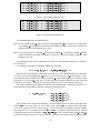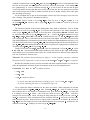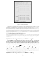
1
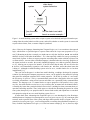
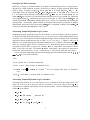
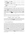
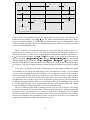
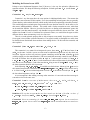
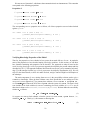
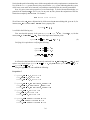
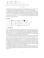
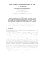
Model Checking Cooperation, Knowledge, and Time
— A Case Study
Wiebe van der Hoek and Michael Wooldridge
Department of Computer Science
University of Liverpool,
Liverpool L69 7ZF, United Kingdom.
wiebe,m.j.wooldridge @csc.liv.ac.uk
Abstract
Alternating-time Temporal Logic (ATL) is a logic developed by Alur, Henzinger, and Kupferman for reasoning about coalitional powers in multi-agent systems. Since what agents can achieve
in a specific state will in general depend on the knowledge they have in that state, in an earlier
paper we proposed ATEL, an epistemic extension to ATL which is interpreted over Alternating-time
Temporal Epistemic Transition Systems (AETS). The logic ATEL shares with its ancestor ATL the
property that its model checking problem is tractable. However, while model checkers have been
implemented for ATL, no model checker yet exists for ATEL, or indeed for epistemic logics in general. The aim of this paper is to demonstrate, using the alternating bit protocol as a detailed case
study, how existing model checkers for ATL can be deployed to verify epistemic properties.
1 Introduction
We begin with an informal overview of this paper, intended for a non-computing audience; we then
give a detailed formal introduction.
This paper is about the use of computers for automatically proving properties of game-like multiagent encounters. Specifically, we describe how a technique called model checking can be used for this
purpose. Model checking is an approach that was developed by computer scientists for verifying that
computer programs are correct with respect to a specification of what they should do. Model checking
is the subject of considerable interest within the computer science community because it is a fully automatic verification technique: that is, it can be fully automated by computer, and a computer program
(a model checker) can be used to verify that another computer program is correct with respect to its
specification.
Model checking systems take as input two entities: a system, whose correctness we wish to verify,
and a statement from the requirements that we wish to check to hold in the system. For example,
suppose we had written a computer program that was supposed to control a lift (elevator). Some
typical requirements for such a system might be that ‘two lifts will never react on the same call’, and
‘eventually, every call will be answered by a lift’. A model checking program would take as input the
lift control program, these requirements (and potentially others), and would check whether or not the
claims were correct with respect to the program; if not, then model checking programs give a counter
example, to illustrate why not (see Figure 1). The latter property is of course especially useful in
debugging programs.
Most existing model checking systems allow claims about the system’s behaviour to be written in
the language of temporal logic, which is well-suited to capturing the kind of requirement expressed
1
claim about
system behaviour
system
model
checker
"yes, the claim
is valid"
"no, the claim is not valid:
here is a counter example..."
Figure 1: A model checking system takes as input a system to be checked, and logical formulae representing claims about the behaviour of the system, and verifies whether or not the system is correct with
respect to these claims; if not, a counter example is produced.
above. However, the language Alternating-time Temporal Logic (ATL) is an extension to the temporal
logic, which allows a system designer to express claims about the cooperation properties of a system [2]. Returning to the above example, we might want to verify that ‘the lifts , and can establish
that there is always a lift below the -th floor’. ATL is thus especially suitable for strategic reasoning in
many kinds of games: it allows to express properties concerning what certain coalitions of players can
or cannot achieve. An even richer verification language is obtained when also knowledge properties of
the agents involved are at stake: the recently introduced language ATEL adds an epistemic dimension
to ATL, allowing one to express for instance ‘if one lift knows that the other lifts are all below the
-th floor, it will immediately respond to a call from the
-th floor, and let the others know that
it doing so’. Although no model checking systems exist for ATEL, a model checker for ATL has been
implemented [3, 1].
Thus, our aim in this paper is to show how model checking, a technique developed by computer
scientists for showing that computer programs are correct, can be applied to the problem of proving
that game-like multiagent encounters have certain properties. We do this by means of a case study:
the alternating bit protocol. This is a communications protocol that is designed to allow two agents
to reliably communicate a string of bits between each other over a potentially faulty communications
channel. The language ATEL is a natural choice to express properties of the protocol, since a property like ‘the sender and the receiver have a way to achieve that, no matter how the channel behaves,
eventually they know that a particular bit has been received’ is nothing less than a statement about cooperation, knowledge and time. Thus, in this paper, we describe the alternating bit protocol as a finite
state system, then specify ATEL properties that we want to check on this, and explain how we can check
such properties using the MOCHA model checking system for ATL.
In more detail, then, Alternating-time Temporal Logic (ATL) was introduced by Alur, Henzinger,
and Kupferman as a language for reasoning about concurrent game structures [2]. In a concurrent game
structure, nodes represent states of the system, and edges denote possible choices of agents. Thus ATL
generalizes branching time logics, a successful approach to reasoning about distributed computer systems, of which Computation Tree Logic (CTL) is the best known example [5]. In CTL, however, edges
2
between states represent transitions between time points. In distributed systems applications, the set of
all paths through a tree structure is assumed to correspond to the set of all possible computations of a
system. CTL combines path quantifiers “ ” and “ ” for expressing that a certain series of events will
happen on all paths and on some path respectively, with tense modalities for expressing that something
will happen eventually on some path ( ), always on some path ( ) and so on. Thus, for example, by
using CTL-like logics, one may express properties such as “on all possible computations, the system
.
never enters a fail state”, which is represented by the CTL formula
ATL is a generalisation of CTL, in the sense that it replaces the flow of time by the outcome of possible strategies. Thus, we might express a property such as “agent has a winning strategy for ensuring
that the system eventually terminates”. More generally, the path quantifiers of CTL are replaced in ATL
by modalities for cooperative powers, as in: “agents and can cooperate to ensure that the system
. It is not possible to capture
never enters a fail state”, which would be denoted by such statements using CTL-like logics. The best one can do is either state that something will inevitably
happen, or else that it may possibly happen; CTL-like logics have no notion of agency. Incorporating
such cooperative powers in the language makes ATL a suitable framework to model situations where
strategic reasoning is crucial, as in multiagent systems in general [16], and in particular, games [14].
Note that ATL is, in a precise sense, a generalisation of CTL: the path quantifiers (“on all paths. . . ”)
and (“on some paths. . . ”) can be simulated in ATL by the cooperation modalities (“the empty
set of agents can cooperate to. . . ”) and (“the grand coalition of all agents can cooperate to. . . ”).
But between these extremes, we can express much more about what certain agents and coalitions can
achieve.
In [11], we enriched ATL with epistemic operators [7, 13], and named the resulting system Alternatingtime Temporal Epistemic Logic (ATEL). This seems a natural way to proceed: given the fact that ATL
is tailored to reason about strategic decision problems, one soon wants to reason about the information
that the agents have available upon which to base their decisions. ATEL is a succinct and very powerful
language for expressing complex properties of multiagent systems. For example, the following ATEL
formula expresses the fact that common knowledge in the group of agents about is sufficient to
enable to cooperate and ensure : "!#%$ &'() . As another example, involving both a knowledge pre- and post-condition, the following ATEL formula says that, if knows that , then has a
strategy to ensure that * knows — in other words, can communicate what it knows to other agents:
+-,
+32
.$/01(
. For (many) other examples, we refer the reader to [11].
Although the computational complexity of the deductive proof problem for CTL is prohibitively expensive (it is EXPTIME-complete [5, p.1037]), the model checking problem for CTL — the problem of
determining whether a given formula of CTL is satisfied in a particular CTL model — is comparatively
easy: it can be solved in time 4)5(6786:9;6<6= , where 6786 is the size of the model and 6>6 is the size of the
formula to be checked [5, p.1044]. Results reported in [2] and [11] show that the model checking problem remains PTIME-complete when moving to ATL and its epistemic variant ATEL, respectively. The
tractability of CTL model checking has led to the development of a range of CTL model checking tools,
which have been widely used in the verification of hardware and software systems [4]. Using the techniques pioneered in these systems, the MOCHA model checking system for ATL was implemented [3, 1].
However, this tool does not straightforwardly allow one to deal with epistemic extensions, as in ATEL.
The aim of this paper is to demonstrate, by means of detailed case study, how one might put MOCHA to
work in order to check properties in a system where reasoning about knowledge is essential. We verify
properties of a communication protocol known as the alternating bit protocol [9]. In this protocol, the
knowledge that one agent has about the knowledge of the other party is essential.
The remainder of the paper is structured as follows. In Section 2, we briefly re-introduce ATEL,
beginning with a review of the semantic structures that underpin it. In section 3, we give an outline of
the alternating bit protocol, and we show how it is possible to verify ATEL properties of this protocol
MOCHA [3, 1].
3
2 Alternating-time Temporal Epistemic Logic (ATEL)
We begin by introducing the semantic structures used to represent our domains. These structures are
a straightforward extension of the alternating transition systems used by Alur and colleagues to give a
semantics to ATL. Formally, an alternating epistemic transition system (AETS) is a tuple
- 3
,
,
' where:
is a finite, non-empty set of atomic propositions;
# is a finite, non-empty set of agents ;
is a finite, non-empty set of states;
,
89, is an epistemic accessibility relation for each agent — we usually require
that each
$
is an equivalence relation;
gives the set of primitive propositions satisfied in each state;
9 $ !#" is the system transition function, which maps states and agents to the choices
( -,
) is the set of choices
available to these agents. Thus 5$ 1=% & ')( with +*
available to agent when the system is in state $ . If makes choice .* , this means that the next
state will be some $/01-* : which state it exactly will be, depends on the other agents. We
require that this function satisfy the requirement that the system is completely controlled by its
,54
component agents: for every state $23 , if each agent * chooses , then the combined choice
,7698886 ,5
is a singleton. This means that if every agent has made his choice, the system
is completely determined: there is exactly one next state. Note that this requirement implies that
every agent has at least one choice to make in every state: for every $ and every , there is a
;:
, such that <= 5$ = .
We denote the set of sequences over by ?> , and the set of non-empty sequences over
Moreover, and * will be used as variables ranging over the set of agents .
Epistemic Relations
by
A@
.
+ ,
To appreciate the next example, we already stipulate the truth condition for knowledge formulas
, ,
which intuitively is read as ‘agent knows ’. If B is an AETS with its set of states, and an
equivalence on it, then
B
C$ 6 +-,
iff D7$ / 5 $E
,
$ /GF
B
C$ / 6 '=
We sometimes omit B , when it is clear from context. The definition says that what an agent knows
in a state $ is exactly what is true in all the states $ / that cannot be distinguished from $ , by that agent.
Example 1 Consider the following AETS - 3
' (see also Figure 2):
, the set of atoms, comprises just the singleton IH ;
J8 L K is the set of agents consisting of the environment
communicate;
M
N$ $O ;
4
K
and two agents that want to
$
:
H
$
!
:
H
$
$O
$
$ $
$
Figure 2: Closed bullets denote H -states, in open bullets, H is true. The epistemic accessibility relation
of agent is the reflexive closure of the straight lines, that of agent is the reflexive closure of the dotted
lines.
We suppose that K is omniscient: 5$I* C$I* = 6%,
. Agent cannot distinguish $ from $ ! ,
5$I C$ = 5$ C$I:= 5$ C$ = 5$ C$ = . Accessibility for
and also not $ from $ , i.e., ?J !
!
is defined as 5$C$ = 5$C$ = 15$C$ = #5$C$ = ;
!
is such that 5$#*=5 H =7&K iff is odd ( -,
? 9 %$
!#"
);
is given in Figure 3 and explained below.
To understand the example further, we anticipate it may be helpful to understand the model of Figure 2
in fact as three components: the first comprising $ and $ , and the last consisting of $ and $O . This is
how knowledge evolves along the system:
1. Agent 2 has information whether H , in the first component. For the sake of the example, let us
suppose that H is true, so the initial state is $ . Note that we have:
$ +
6 H
!
+
H
+
H
5
+
+
H
!
!
+
=
H
+
5
!
H
+
"
H =
Thus: in $ , agent knows that H , agent does not know H , but knows that knows whether H
(i.e., knows that knows whether H is true or false); moreover, knows that does not know
whether H .
2. Agent then can choose to either send information about the status of H to agent
case there is a transition to either $ or $ ), or to do nothing (leaving the system in
does not know that:
$ , the communication was apparently successful, although
+
6
$
+
H
!
+
H
+
!
+
H
+
!
$ (in which
). In state
H
The environment K can choose the communication to fail, in which case agent ’s action leads us
to $ , where knows H but does not, and moreover agent does not know whether knows H :
6
$
+
+
"
H
!
Finally, $ models a state in which agent
$
6
+
H
+
!
H
+
H
+
H
!
+
!
+
H
+
successfully acknowledged receipt of the message H :
+
!
H
+
+
!
H
+
+
+
!
H
We have given part of the transition function in Figure 3. The description is not complete: we have
for instance not stipulated what the choices are in the H -states, neither did we constrain the options in
the ‘final’ state $ . Let us explain for the initial state $ . In that state, the environment K cannot control
5
whether agent will send the message H (explaining the fact that $ is a member of all of K ’s options
N$ C$ and N$ C$ , leaving the choice for $ so to speak up to agent ), but if the message is sent, K
can control whether the resulting state will be $ (message not arrived) or $ (message arrived). Agent
, on the other hand, has the possibility in state $ either to not send the message H at all (in which case
he chooses N$ ), or to send the message, in which case he cannot control delivery (explaining why ’s
second option in $# is N$ C$ ). Finally, agent has no control over ’s choice at all, it leaves it to the
other agents to choose among N$ C$C$ .
K
5 =
5$ LK=
5 $LK=
K
K
5 =
5$ =
5$ =
N$ C $<N$ C$
N $ <
N$ N $ C$ $ LK
'
'
'
5 =
5$ =
5 $ =
$ N$ <N$C$ N $ C $C$ N $ C $ C$ $ N$ C $C$ N $ C $ N $ <
N$ Figure 3: Partial description of the transition function K , and .
Note that indeed, the system as a whole is deterministic: once all the agents have made their choices
, the resulting state will either be $ (agent choosing N$ , no matter what the others choose), or
$ ( K choosing N$ C$ and
choosing N$C$ ) or $ ( K choosing N$ C$ and choosing N$C$ ).
Further note that no agent has the possibility to alter the truth of H , only the knowledge concerning H is
updated.
in
$ Computations
For two states $ C$ / and an agent , we say that state $ / is an -successor of $ if there exists
a set ./ J 5$ = such that $/ ;./ . Intuitively, if $ / is an -successor of $ , then $/ is a possible
outcome of one of the choices available to when the system is in state $ . We denote by 5$ =
the set of successors to state $ . We say that $ / is simply a successor of $ if for all agents , we
have $/ 5$ 1= ; intuitively, if $ / is a successor to $ , then when the system is in state $ , the agents
can cooperate to ensure that $ / is the next state the system enters.
A computation of an AETS - 3 ' is an infinite sequence of states $C$ such that for all , the state $ is a successor of $ . A computation starting in state $ is referred
to as a $ -computation; if 1 , then we denote by the ’th state in ; similarly,
we denote by 1 and " the finite prefix $ C$ and the infinite suffix $ C$ of
@ 8
8
respectively. We use to concatenate a sequence of states with a state $ to a new sequence
$ .
Example 1 (ctd). Possible computations starting in $ in our example are $ C$ C$ ( decides
not to sent the message); $ C$ C$C$C$ C$ ( sends the message at the second step, but it never
arrives), and for instance $ C$ C$C$C$C$C$ (after two steps, sends the message five times in
a row, after the fourth time it is delivered, and immediately after that obtains an acknowledgement).
Note that these computations do not alter the truth of H , but only knowledge about the status of H : in
this sense, the dynamics can semantically be interpreted as changing accessibility relations, and not the
states themselves.
6
Strategies and Their Outcomes
Intuitively, a strategy is an abstract model of an agent’s decision-making process; a strategy may be
thought of as a kind of plan for an agent. By following a strategy, an agent can bring about certain
,
,
states of affairs. Formally, a strategy for an agent is a total function @ $
,
, 8
$= 5$ 1= for all
. Given a set
> and $
which must satisfy the constraint that 5
,
of agents, and an indexed set of strategies ! ( 6" , one for each agent , we
define 5$ ! = to be the set of possible outcomes that may occur if every agent follows the
,
corresponding strategy , starting when the system is in state $ J . That is, the set 5$ ! = will
contain all possible $ -computations that the agents can “enforce” by cooperating and following the
strategies in ! . Note that the “grand coalition” of all agents in the system can cooperate to uniquely
determine the future state of the system, and so 5$ = is a singleton. Similarly, the set 5$ =
is the set of all possible $ -computations of the system.
Alternating Temporal Epistemic Logic: Syntax
Alternating epistemic transition systems are the structures we use to model the systems of interest to
us. Before presenting the detailed syntax of ATEL, we give an overview of the intuition behind its key
constructs. ATEL is an extension of classical propositional logic, and so it contains all the conventional
connectives that one would expect to find: (“and”), (“or”), (“not”), $ (“implies”), and so on. In
,
addition, ATEL contains the temporal cooperation modalities of ATL, as follows. The formula & where is a group of agents, and is a formula of ATEL, means that the agents can work together
(cooperate) to ensure that is always true. Similarly, & means that can cooperate to ensure
that is true in the next state. The formula &'( means that can cooperate to ensure that remains true until such time as is true — and moreover, will be true at some time in the future.
An ATEL formula, formed with respect to an alternating epistemic transition system B9 -
' , is one of the following:
(S0) (S1)
, where H
H
is a primitive proposition;
(S2) or ; , where and are formulae of ATEL;
(S3) & , &'
, or & , where is a set of agents, and and are formulae of
ATEL;
(S4)
+-,
, where is an agent, and is a formula of ATEL.
Alternating Temporal Epistemic Logic: Semantics
We interpret the formulae of ATEL with respect to AETS, as introduced in the preceding section. Formally, if B is an AETS, $ is a state in B , and is a formula of ATEL over B , then we write B C$ 6 to mean that is satisfied (equivalently, true) at state $ in system B . The rules defining the satisfaction
relation 6 are as follows:
B
C$ 6 B
C$ 6 H iff H
B
C$ 6 iff B C$ 6 : ;
B
C$ 6 5$=
(where H9= );
iff B C$ 6 or B C$ 6 ;
7
B C$ 6 & iff there exists
a set of strategies '! , one for each 5$ ! = , we have B 6 ;
a set of strategies '! , one for each B C$ 6 &' iff there exists
'6 for all ;
5$ ! = , we have B that for all
! , one for each , such
B C$ 6 & ( iff there exists a set of strategies '
'6 , and for all ,
, we have
5$ ! = , there exists some such that B B '6 ;
,
+ ,
B C
$ 6
iff for all $ / such that $0 $ / : B C$ / 6 .
, such that for all
, such that for all
Before proceeding, we introduce some derived connectives: these include the remaining connectives
of classical propositional logic ( , .$ ; and 5.$ = 5 %$ '= ).
As well as asserting that some collection of agents is able to bring about some state of affairs, we
can use the dual “ ” to express the fact that a group of agents cannot avoid some state of affairs.
Thus & expresses the fact that the group cannot cooperate to ensure that will never be true;
the remaining agents in the system have a collection of strategies such that, if they follow them, may
eventually be achieved. Formally, is defined as an abbreviation for &' , while ;
, and so on. Finally, we generally omit set brackets inside
is defined as an abbreviation for &'
cooperation modalities, (i.e., writing 0# * instead of # * ), and we will usually write rather
than .
Example 1 (ctd). In Example 1, the grand coalition can achieve that the agents have mutual knowledge
about the status of H , but this cannot be achieved without one of its members. We can capture this
+
+
+ +
+ +
property in ATEL as follows, letting denote H
H
H
5H :
!
$ 6 K : K !
K (;
!
First of all, note that is only true in $ . Now, to explain the first conjunct in the displayed formula,
it is easy to see that the computation $ C$C$C$ can be obtained by letting every agent play a
suitable strategy. To see that, for instance, K ( is true in $ , note that agent has the power to
always choose option N$ , preventing the other agents from having a strategy to reach $ .
3 The Alternating Bit Protocol
We now present a case study of model checking an ATEL scenario, in the form of the bit transmission
problem. We adapt our discussion of this problem from [13, pp.39–44]. The bit transmission protocol
was first studied in the context of epistemic logic by Halpern and Zuck [9]. In game theory, similar
problems are studied as the ‘Electronic Mail Game’ ([15]). The basic idea is that there are two agents, a
sender B and a receiver , who can communicate with one another through an unreliable communication environment. This environment may delete messages, but if a message does arrive at the recipient,
then the message is correct. It is also assumed that the environment satisfies a kind of fairness property,
namely that if a message is sent infinitely often, then it eventually arrives. The sender has a sequence
of bits that it desires to communicate to the receiver; when the receiver receives the
! C( .
bits, it prints them on a tape , which, when has received number of G* ’s, is
The goal is to derive a protocol that satisfies the safety requirement that the receiver never prints incorrect bits, and the liveness requirement that every bit will eventually be printed by the receiver.
More formally, given an input tape
, with the * from some alphabet H , and
a network in which deletion errors may occur but which is also fair, the aim is to find a protocol for
B and
that satisfies
8
safety — at any moment the sequence
liveness — every
*7
written by
is a prefix of
will eventually be written by
; and
.
Here, the alphabet for the tape is arbitrary: we may choose a tape
over any symbols. In our case
study, we will choose H 1 . The obvious solution to this problem involves sending acknowledgement messages, to indicate when a message was received. Halpern and Zuck’s key insight was to
recognise that an acknowledgement message in fact carries information about the knowledge state of
the sender of the message. This motivated the development of the following knowledge-based protocol.
), the sender transmits it to the receiver. However, it cannot stop
After obtaining the first bit (say at this point, because for all it knows, the message may have been deleted by the environment. It thus
continues to transmit the bit until it knows the bit has been received. At this point, the receiver knows
the value of the bit that was transmitted, and the sender knows that the receiver knows the value of
the bit — but the receiver does not know whether or not its acknowledgement was received. And it is
important that the receiver knows this, since, if it keeps on receiving the bit 1, it does not know how to
interpret this: either the acknowledgement of the receiver has not arrived yet (and the received 1 should
be interpreted as a repetition of the sender’s sending ), or the receiver’s acknowledgement had indeed
arrived, and the 1 that it is now receiving is the next entry on the tape, which just happens to be the
same as . So the sender repeatedly sends a second acknowledgement, until it receives back a third
acknowledgement from the receiver; when it receives this acknowledgement, it starts to transmit the
next bit. When the receiver receives this bit, this indicates that its final (third) acknowledgement was
received.
A pseudo-code version of the protocol is presented in Figure 4 (from [13, pp.39–44]). Note that we
+
write * as a shorthand for “the value of bit N* ”. Thus 5 *= means that the receiver ( ) knows the
value of bit * . The variables and range over the natural numbers. A command such as
“send until * ” for a boolean * must be understood as: the process is supposed to repeatedly send ,
until the boolean becomes true. The boolean is typically an epistemic formula: in line B for instance,
!
B keeps on sending , until it knows that
has received .
The protocol of Figure 4 is sometimes called a knowledge-based program [8], since it uses constructs (boolean tests and messages) from the epistemic language. Of course, conventional programming languages do not provide such constructs. So, let us consider how the protocol of Figure 4 can be
translated into a normal program, on the fly also explaining the name of the protocol.
+
The first insight toward an implementation tells us that messages of the form * ( B )
can be seen as acknowledgements. Since there are three such messages, on lines B and ,
!
respectively, we assume we have three messages: G! and . So, for instance, in B& , ‘send
+ + 5 = ” ’ is replaced by ‘send ! ’. Next, we can replace the Boolean conditions of type
“
+
* by the condition that is received. Thus, B gets replaced by “send ! until is received”.
Thus, the lines B B , and of Figure 4 become, respectively:
!
!
B send
send
!
B !
send
send
!
until is received
until is received
until ! is received
until is received
@
Now, the alternating bit protocol is obtained by the following last step. Sender can put information
on which bit he sends by adding a “colour” to it: say a to every '* for even , and a for every odd
8
8
. So the new alphabet H G/ becomes ;6 H 6 H We also now need only
two acknowledgements: and 1 . Thus, the idea in the alternating bit protocol is that B first
1
Note that the specification for this protocol in terms of epistemic operators would not require knowledge of depth four
anymore, since some of the knowledge now goes in the colouring.
9
Sender
B
B +
BG B while true do
read + + 5 +
=
send until
+ + +
send “
5 = ” until
B !
B +
end-while
+ +
5
5 =
end-Sender
Receiver
!
+
when 5 = set +
while true do
write +
+ + +
send “ 5 = ” until + + + +
send “ 5 0= ” until
+
end-while
end-Receiver
5
=
@
=
Figure 4: The bit transmission protocol (Protocol A).
8
8
sends . When it receives , it goes on to the next state on the tape and sends . of course
sees that this is a new message (since the colour is different), and acknowledges the receipt of it by
8
, which B can also distinguish from the previous acknowledgement, allowing it to send
next.
!
H / 1 ,
The only function we need is thus a colouring function H $
defined by
8
5 =+
8
if is even
otherwise.
The protocol thus obtained is displayed in Figure 5.
3.1 Modelling the Protocol
In the Alternating Epistemic Transition System that we build for the protocol, we consider three agents:
Sender B , Receiver and an environment K . We are only interested in the knowledge of and B .
Naturally, the local state of B would be comprised of the following information: a scounter and atoms
8
8
8
8
for every two atoms rcvd and rcvd , where
sent * , sent *
H 8 , and, finally,
8
* is the -th bit of the input tape, and and are the two acknowledgement messages. This
however would lead to an infinite system, because of the counter used. Hence, we don’t consider this
counter as part of the local state. Moreover, we also abstract from the value . In other words, in the
H ). We do the same for .
local state for B , we will identify any and & / ( " &/ There is another assumption that helps us reduce the number of states: given the intended meaning
8
8
), we can impose as
of the atoms sent (the last bit that has been sent by B is of the form
8
8
a general constraint that the property sent sent
should hold: agent B can only have
8
8
sent one kind of message as the last one. The same applies to the atom-pairs (sent ,sent ),
8
8
8
8
(rcvd ,rcvd
) and (rcvd ,rcvd ).
There are in general two ways one could deal with such a constraint. One would be not to impose
it on the model, but instead verify that the protocol adheres to it, and prove, for instance, that there is
10
Sender
B
B +
BG B while true do
read send 5 " B !
+
end-while
(=
until 50 (=
is received
end-Sender
Receiver
when 5 " = is received while true do
write send 50 = until 5 " !
+ end-while
end-Receiver
= is received
Figure 5: The alternating bit protocol.
no run in which one of the agents has just sent (or received) two messages of a pair in a particular state
(such an approach is undertaken in [12], where the model is divided in “good” and “bad” states). Since
here we are more interested in epistemic properties of the protocol, rather than proving correctness
properties of the channels (e.g., no two messages arrive at the same time) we choose the second option,
and define a model that incorporates the constraint on the pairs already.
In summary, the states in our model will be represented as four-tuples
)
6
# $I*
where:
#
. ; and
2
$* , where
,
E, , is the name of the state, which is just the decimal representation of the
binary number the state corresponds to (so for instance, $ 6 ).
We furthermore use variables :C$ C$ C $
as follows:
!
to range over states. The interpretation of the atoms are
ssx being true means that the last bit that
sent was of type
B
sra says that the last bit he has received is rrx means that
8
8
8
;
;
has recently received a bit of type
rsa indicates that he just sent 8
; and
.
Obviously, given the constraint mentioned above, an atom like sra being false indicates that the last
8
bit that B received is . Thus, for instance, the state $ 6 encodes the situation in which
8
8
the last bit that B has sent is of type
, the last bit he received was , the last bit received was
8
8
, and he has recently sent .
11
q4
<0, 1 | 0, 0>
q0
<0, 0 | 0, 0>
q8
<1, 0 | 0, 0>
q5
<0, 1 | 0, 1>
q10
<1, 0 | 1, 0>
q7
<0, 1 | 1, 1>
q11
q15
<1, 1 | 1, 1>
<1, 0 | 1, 1>
initial state
Key: states are of the form <ssx, sra | rrx, rsa>.
Figure 6: Runs of the alternating bit protocol: arrows indicate successor states. Note that there are
states that are not reachable, such as 6 . The Sender cannot distinguish states that are placed
on top of each other; similarly, for the Receiver, horizontally placed states are indistinguishable. Thus
columns represent equivalence classes of B -indistinguishable states, while rows represent equivalence
classes of -indistinguishable states.
There is a natural way to model the epistemics in a system like that just described, since it is a
special case of an interpreted system (cf. [7]), where the assumption rules that agents (exactly) know
what their own state is, in other words, an agent cannot distinguish the global state from (i.e.,
,
.
) if his local part in those states, and are the same. In our example it would mean for B
that two states $ >6
and $ 6 are epistemically
!
indistinguishable for him if and only if $ B = = = $ B . Thus B knows
!
what the last bits are that he has sent and received, but has no clue about the last bits that were sent or
received by . The same reasoning determines, mutatis mutandis, the epistemic accessibility for agent
.
In [2], Alur et al. identify several kinds of alternating systems, depending on whether the system
is synchronous or not, and on how many agents “really” determine the next state. They also model
a version of the alternating bit protocol (recall that in ATL no epistemics is involved) for a sender B
and an environment K . Their design-choice leads them to a turn-based asynchronous ATS where there
is a scheduler who, for every state, decides which other agent is to proceed, and the other agents do
not influence the successor state if not selected. As the name suggests, this in in fact an asynchronous
modelling of the communication, which we are not aiming for here. In our modelling, if one of B and
(or both) sends a message, it does not wait and then find out whether it has been delivered: instead,
it keeps on sending the same message until it receives an acknowledgement.
The way we think about the model is probably closest to [2]’s lock-step synchronous ATS. In such
an ATS, the state space is the Cartesian product of the local spaces of the agents. Another constraint that
[2] imposes on lock-step synchronous ATSs is that every agent uniquely determines its next local state
(not the next global state, of course), mirroring systems where agents just update their own variables.
However, this assumption about determinacy of their own local state is not true in our example: the
communicating agents cannot control the messages they receive.
12
Modelling the Protocol as an AETS
Perhaps a more fundamental departure from [2] however, is the way the epistemics influences the
,
transition relation. We adopt the following assumption, for both agents ;B (recall that $ iff $ ).
Constraint 1
,
$0
5$ 1=)J 5 : =
implies Constraint 1 says that agent have the same options in indistinguishable states. That means that
agents have some awareness of their options. If we aim at modelling rational agents, then we generally
assume that they make rational decisions, which usually boils down to optimising some utility function.
This would imply that a rational agent always makes the same decision when he is in the same (or, for
that matter, indistinguishable) situation. This would entail a further constraint on runs, rather than
on the transition function. However, given the fact that we are dealing with autonomous agents, this
requirement is not that natural anymore: why shouldn’t an agent be allowed to choose once for , and
another time for / ? Even if we would not have epistemic notions, we would allow the agent to make
different choices when encountering exactly the same state.
There is a second epistemic property that we wish to impose on our model. It says that every choice
for an agent is closed under epistemic alternatives. If an agent is unable to distinguish two states, then
he should also not discriminate between them when making choices. We first state the constraint, and
then explain it.
Constraint 2 If
5 1= C$
/ $
3./
and
$ ,
$
!
, then
$
3./
!
,
This constraint is very natural in an interpreted system, where $ iff ’s local states in $ $
!
and $ are the same. In such a system, we often want to establish that agents can only alter their own
!
local state. Suppose we have two processes, agent controlling variable and controling
(both
!
variables ranging over the natural numbers). If has to model that can only control his own variables,
he could for instance have an option to make equal to 7, and an option to make it 13 ( 5$ = 5 " =6 = >5 " = 6 ), but he should not be allowed to determine by himself that the
,
):
next state be one in which is 7 and at the same time being at most 20 ( 5 1=<6 !
!
the latter constraint should be left to process .
In the following, let N/ G/ be variables over the booleans. Moreover, let # receive
their natural interpretation. Remember that )6 = -6 iff the last bit sent by
8
8
8
, the last acknowledgement received is , the last bit received by is
and
B is of the form
8
the last acknowledgement sent by is .
A next assumption is that sending a message takes some time: it is never the case that a message is
sent and received in the same state.
5 '= $ B
5 $
Constraint 3 Let
$ /
be a successor of $ (that means: there are and
?6
6 - N$/ . Then:
= and = 5$ LK= with if
$0
# 6 and
$ / # / 6 / / then if
$0
# 6 and
$/ /G/6/ then G/
/ such that
.
.
Definition 1 We say that an agent does not have control over the bit if for all $ , we have: if
,
,
,
, if $ / # 6 , then also 611+ .
5$ 1= , then for any $ / 3
Constraint 4 Given our terminology for states )6
# , agent B has no control over
has no control over #
and the environment K has no control over
#
, agent
.
13
B
B
B
50
50
50
50
B
6 1 1
-611
6 1 1
-6 1 1
B =
B =
B =
B =
/ 6 / / 6 / G/ 6 / / 6 G/ / 6 / / 6 / / 6 / / 6 / / / ')
')
')
')
/ / / / / / Figure 7: The transition function for
50 #
50 # 50 # 50 # 6 6 6 6 =
=
=
=
& 6/ 6 /&
/ / 6 / 6 / / / 6 / 6 / /&
G/6 / 6 /&
/ G/
/
/
/
/
/ / / (B
(B
B
/ Figure 8: The transition function for
The transition function of
B
establishes that:
8
8
and received its acknowledgement , it moves on to a state where
) if B has recently sent
8
it is sending
, being unable to determine what kind of messages it will receive, and likewise
unable to influence what happens to ’s state;
) if
8
8
8
, but still receiving , being
is in the process of sending
, it continues to send
unable to determine what kind of messages it will receive, and likewise unable to influence what
happens to ’s state.
B
The motivation for the clauses B and B are similar, as is the transition function for
give in Figure 8.
It is tempting to attempt to combine B and B into one clause
, which we
B
50 611 B =
/ 6 / / 6 / / / However, there still should be a difference between the two. The transition in B can be described
8
8
as “I have received acknowledgement now, so I proceed to send a new
from the tape”, where
8
is not acknowledged yet, so I have to repeat
as the transition at B should be labelled “My message
8
to send this old version of
once more”. In other words, the transition at B has as a side effect that
, whereas the transition at B keeps B at the same position of the tape.
B advances on the tape
We finally concentrate on the transition function of the environment K , as displayed in Figure 9. As
a first approach to this transition function, consider the following clause:
K
50 # 6 LK=
/&
/ / /& 6 N/ 6 /N/
6 / 6 / /
6 / 6 / /
6 N/ 6 / N/
This transition rule expresses the following. The environment leaves the control of the first state
variable to the other agents, as well as that of the variable : it cannot control what either
of the other agents has sent as a latest message. On the other hand, K completely controls whether
messages arrive, so it is in charge of the bits and . If, using this transition function, K would
8
8
for instance choose the first alternative, / 6 / 6 / / , it would decide that and
get delivered. However, this is in a sense too liberal: we do not, for instance, want the environment to
14
establish a transition from a state 61 to any state / 6 / , since it would mean that in the
8
8
first state has recently sent and B has received it, and in the next state is still sending 8
but “spontaneously”, B receives a different message . It can of course be the case that an agent
is receiving another message than that most recently sent to him, but once any agent has received the
most recent message sent to him, he cannot from then on receive another message if the other agent
does not change its message.
So, the condition that we put on the environment is that it may loose messages, but it will never
alter a message. This property is formalised as follows.
Constraint 5 Suppose state $ is of type 6#1 . Then for any the form /G/6 N/ . Similarly, if $ is of type # 6 , then any
/ 6 / / .
5 = , any
$/
is of
should be of the form
$ LK
in
$ /
The transition function for K basically distinguishes three kinds of transitions. First of all, K
and K are on states of type 6 . It is obvious that Constraint 5 only allows transitions to
states of type / 6 / , for which K is not in the power of determining / or / . Secondly, there
are transitions from states of type 6 / with c : c’ (clauses K LK LK
and K ) or of type
1 6 / ( K LK LK and K ), with : / . Consider the first case, i.e., $? 6 / (the other
case is analogous). This is a state where Receiver has received the right , but Sender still waits for the
right acknowledgement. Environment can now choose whether this acknowledgement will arrive: so it
can choose between the states of type 6 / / (acknowledgement still not arrived) and those of
type /6 / / (acknowledgement arrived), which is equivalent to saying that the resulting states
or either of type 6 / / or of type 6 / / .
Finally, we have the cases K LK LK and K . Here, the argument $ is of type 611 , where
: and :
. This means that both Sender and Receiver are waiting for the “right” acknowledgement, and the receiver can choose to have none, one, or both of them to be delivered. This explains the
four sets of alternatives for these cases.
Theorem 1 The transition function displayed in Figures 7, 8 and 9 together constitute a transition
6
6
function for an ATS, in particular, we have for any state $ , that 5$ B = 5$ = 5$ LK= is a singleton.
Besides the constraints we have put on to our model and on the transition function, we also have to
make the requirements of fairness (by the environment) on the set of all computation runs.
Constraint 6 Let 1. 5$ B'=)
2. 5$ =
9 %$
be defined as follows:
! "
3. 5$ LK= is defined as follows:
(a) for the states $ of which the binary encoding is not 4, 7, 8 or 11, 5$ LK=
(b) for the remaining four states, is as defined in Figure 10.
5 =
J $ LK
Let us explain the fairness constraint , the others are similar. When comparing with K ,
we see that removes 6 / 6 N/+ from 50 -6 LK= : which is exactly the choice
that would not take us any further in a computation step: given the state -6 , we know that
8
8
from . Until these
B is waiting to receive from , who, in his turn, awaits to receive
8
messages are not received, B and will keep on doing what they do in the given state: send
8
8
and , respectively. If the environment will not eventually deliver , the process will not really
make progress any more. We do not have to impose such a constraint on for instance K , defined on
8
has received an acknowledgement for his message , and hence he will
6 : here, the Sender
8
, leading us to a state of type 6N/ / / .
continue to send an
15
K
K
K
6 LK=
K
50 36 LK=
K
50
6 LK=
50
6 LK=
K
50
50 K
6 L K=
6 L K=
5036 LK=
5036 LK=
5036 LK=
K
6 LK=
5036 LK=
50 36 L K=
50 36 L K=
K
K
K
50 36 LK=
K
50 K
6 L K=
6 L K=
K
K
50 K
50 50 6 / 6 6 / 6 6 / 6 6 / 6 6 / 6 6 / 6 6 / 6 6 / 6 6 / 6 6 / 6 6 / 6 6 / 6 6 / 6 6 / 6 6 / 6 6 / 6 6 / 6 6 / 6 6 / 6 6 / 6 6 / 6 6 / 6 6 / 6 6 / 6 6 / 6 6 / 6 6 / 6 6 / 6 6 / 6 6 / 6 6 / 6 6 / 6 6 / 6 6 / 6 6 / 6 6 / 6 / N/
,
/ / / / / / ,
/ / / N/
N/
N/
N/
N/
,
/ ,
/ / / / N/
/ N/
/ / / / / N/
N/
N/
N/
N/
N/
,
,
,
,
/ Figure 9: The transition function for
K
Modelling the Protocol with MOCHA
We now consider an implementation of the protocol and the automatic verification of its properties via
model checking. We make use of the MOCHA model checking system for ATL [3, 1]. MOCHA takes as
input an alternating transition system described using a (relatively) high level language called REAC TIVEMODULES. MOCHA is then capable of either randomly simulating the execution of this system, or
else of taking formulae of ATL and automatically checking their truth or falsity in the transition system.
16
50
50
50
50
6 6 6 6 "=
"=
"=
"=
6 / 6 6 N/ 6 6 / 6 6 / 6 / / / /
Figure 10: The transition function for A key issue when model checking any system, which we alluded to above, is that of what to encode within the model, and what to check as its properties. In general, the model that is implemented
and subsequently checked will represent an abstraction of the actual system at hand: the model designer must make reasoned choices about which features of the system are critical to the fidelity of the
model, and which are merely irrelevant detail. Our first implementation, given in Figure 11, is a good
illustration of this issue. In this model, we do not even attempt to model the actual communication
of information between the sender and receiver; instead, we focus on the way in which the acknowledgement process works, via the “colouring” of messages with alternating binary digits, as described
above. This leaves us with a simple and elegant model, which we argue captures the key features of the
protocol.
Before proceeding, we give a brief description of the MOCHA constructs used in the model (see [1]
for more details). The greater part of the model consists of three modules, which correspond to the
agents Sender, Receiver, and Environment. Each module consist of an interface and a number
of atoms, which define the behaviour of the corresponding agent. The interface part of a module
defines two key classes of variables 2 :
interface variables are those variables which the module “owns” and makes use of, but which
may be observed by other modules;
external variables are those which the module sees, but which are “owned” by another
module (thus a variable that is declared as external in one module must be declared as an
interface variable in another module).
Thus the variable ssx is “owned” by the sender, but other modules may observe the value of this
variable if they declare it to be external. The Environment module in fact declares ssx to be
external, and so observes the value of ssx.
Within each module are a number of atoms, which may be thought of as update threads. Atoms
are rather like “micro modules” — in much the same way to regular modules, they have an interface
part, and an action component, which defines their behaviour. The interface of an atom defines the
variables it reads (i.e., the variables it observes and makes use of in deciding what to do), and those
it controls. If a variable is controlled by an atom, then no other atom is permitted to make any
changes to this variable3 . The behaviour of an atom is defined by a number of guarded commands,
which have the following syntactic form.
[] guard -> command
Here, guard is a predicate over the variables accessible to the atom (those it reads and controls),
and command is a list of assignment statements. The idea is that if the guard part evaluates to true,
then the corresponding command part is “enabled for execution”. At any given time, a number of
2
MOCHA also allows an additional class of private (local) variables, which are internal to a module, and which may
not be seen by other modules. However, we make no use of these in our model.
3
Again, there is actually a further class of variables that an atom may access: those it awaits. However, again, we make
no use of these in our model, and so we will say no more about them.
17
module Sender is
interface ssx : bool
external sra : bool
atom controls ssx reads ssx, sra
init
[] true -> ssx’ := false
update
[] (ssx = false) & (sra = false) -> ssx’ := true
[] (ssx = false) & (sra = true) -> ssx’ := false
[] (ssx = true) & (sra = false) -> ssx’ := true
[] (ssx = true) & (sra = true) -> ssx’ := false
endatom
endmodule -- Sender
module Receiver is
interface rsa : bool
external rrx : bool
atom controls rsa reads rrx
init
[] true -> rsa’ := true
update
[] true -> rsa’ := rrx
endatom
endmodule -- Receiver
module Environment is
interface rrx, sra : bool
external ssx, rsa : bool
atom controls rrx reads ssx
init
[] true -> rrx’ := true
update
[] true -> rrx’ := ssx
endatom
atom controls sra reads rsa
init
[] true -> sra’ := true
update
[] true -> sra’ := rsa
endatom
endmodule -- Environment
System := (Sender || Receiver || Environment)
Figure 11: Modelling the alternating bit protocol for MOCHA
guards in an atom may be true, and so a number of commands within the atom may be enabled for
execution. However, only one command within an atom may actually be selected for execution: the
various alternatives represent the choices available to the agent.
Assignment statements have the following syntactic form.
18
var’ := expression
On the right-hand side of the assignment statement, expression is an expression over the variables
that the atom observes. On the left-hand side is a variable which must be controlled by the atom. The
prime symbol on this variable name means “the value of the variable after this set of updates are carried
out”; an un-primed variable means “the value of this variable before updating is carried out”. Thus the
prime symbol is used to distinguish between the value of variables before and after updating has been
carried out.
There are two classes of guarded commands that may be declared in an atom: init and update.
An init guarded command is only used in the first round of updating, and as the name suggests, these
commands are thus used to initialise the values of variables. In our model, the one atom within the
Sender module has a single init guarded command, as follows.
[] true -> ssx’ := false
The guard part of this command is simply true, and so this guard is always satisfied. As this is the
only guarded command in the init section of this atom, it will always be selected for execution at
the start of execution. Thus variable ssx will always be assigned the value false when the system
begins execution.
The update guarded commands in the Sender atom define how the ssx variable should be
updated depending on the values of the ssx and sra variables: essentially, these update commands
say that when the same bit that has been sent has been acknowledged, the next bit (with a different
“colour”) can be sent. It is instructive to compare the four guarded commands that define the behaviour
of this atom with the transition function for the sender, as defined in Figure 7.
The behaviour of the Receiver module is rather similar to that of Sender; however, in the
Environment module there are two atoms. These atoms are responsible for updating the rrx and
sra variables, respectively. Thus, for example, the first atom simply passes on the value of the ssx
variable directly to rrx.
Finally, following the definition of the Environment module is the definition of the System
itself. The one-line declaration says that System is obtained from the parallel composition of the
Sender, Receiver, and Environment modules. The properties that we establish through model
checking are thus properties of System. We will write System 6 to mean that the property
is true in all the states that may be generated by System, where is an ATEL formula over the
propositional variables M ssx sra rrx rsa , which have the obvious interpretation.
Notice that in our first version of the protocol, illustrated in Figure 11, we have designed the environment so that communication of the colouring bits and the corresponding acknowledgement messages is both safe, (in that bits are never transmitted incorrectly), and immediate (the environment
always immediately passes on bits it has received: the communication delay between, for example, an
acknowledgement being sent by the receiver and the acknowledgement being received by the sender
is a single round). Of course, this does not correspond exactly with the definition of the AETS given
earlier, because the AETS permitted the environment to lose messages, and hence to allow states to be
stuttered. In fact, the system in Figure 11 implements the protocol with the weak fairness assumptions
described earlier.
We can easily amend the MOCHA model to allow for stuttering, by simply making the two atoms
that define the environment’s behaviour to be lazy. This is achieved by simply prefixing the atom
definitions with the keyword lazy. The effect is that in any given round, a lazy atom which has a
number of commands enabled for execution need not actually choose any for execution: it can “skip”
a round, leaving the values of the variables it controls unchanged. In particular, a lazy atom may
stutter states infinitely often, never performing an update. In the case of the environment, this means
that messages may never be delivered. We refer to the system containing the standard Sender and
Receiver definitions, together with the lazy version of the Environment, as Lazy.
19
module Environment
interface rrx, sra : bool
external ssx, rsa : bool
atom controls rrx reads rrx, ssx
init
[] true -> rrx’ := true
update
[] true -> rrx’ := ssx
[] true -> rrx’ := true
[] true -> rrx’ := false
endatom
atom controls sra reads sra, rsa
init
[] true -> sra’ := true
update
[] true -> sra’ := rsa
[] true -> sra’ := true
[] true -> sra’ := false
endatom
endmodule -- Environment
Figure 12: A faulty environment.
Finally, the two variations of the system that we have considered thus far are both safe, in the
terminology we introduced above, in the sense that if a message is delivered by the Environment,
then it is delivered correctly. We define a third version of the protocol, which we refer to as Faulty,
in which the environment has the choice of either delivering a message correctly, or else delivering it
incorrectly. The definition of the Environment module for the Faulty system is given in Figure 12.
3.2 Verifying Properties of the Model with MOCHA
Before giving specific formulae that we establish of System, we will list some axiom schemas that
correspond to properties of the class of systems we study. First, we have a property that corresponds to
Constraint 1:
Proposition 1 For all B , and for all , System 6 0 $
+-,
0 Recall that 01 means that can achieve that is true in the next state — no matter what
the other agents do. This just means that the agent has some choice A/ 5$ = such that is
true in every member of / . Constraint 1 guarantees that this / will be an option for in every
state similar to $ , for . Note that this does not mean that the agent will achieve the same in all
accessible states: consider four states $ C$ , with the atom true in just $ and $ , and in $ !
,
and $ . Suppose 5$ 1= 8N$ C$ N$C$ and $2
, so that 5 = < 5$ 1= . This transition
!
function guarantees that $ 6 01 . Moreover suppose that for agent * 5$ * = N$ C$ and
!
5 *=)
N$ C$ . Now it holds that if chooses the option N$ C$ ! in $ , due to * ’s options, -
will hold in the next state, while if makes the same choice in state , will hold in the next state.
This is not in contradiction with Proposition 1, however: all that can guarantee in $ is , not .
Next, we have a property that corresponds to Constraint 2:
Proposition 2 For all B , and for all , System 6 0 $
20
0 +-,
Proposition 2 reflects our assumption that agents can only modify their own local state: if an agent can achieve some state of affairs in the next state, it must be because he makes some decisions on his
local variables, and these are known by agent .
Proofs of these properties are very straightforward, and we leave them to the reader. We now move
on to the specific properties we wish to model check. The first proposition mirrors Constraint 3:
Proposition 3
1. System 6 5 ssx rrx= $
5 2. System 6 5 ssx rrx = $
3. System 6 5 rsa sra= $
5
4. System 6 5 rsa sra = $
ssx $
rrx=
5 ssx $
rsa $
rrx=
sra=
5 rsa $
sra=
The first two of these formula, when translated into the textual form of
are as follows.
ATL
formulae required by
MOCHA,
atl "f01" <<>> G (ssx & rrx) =>
[[Sender,Receiver,Environment]] X (˜ssx => rrx) ;
atl "f02" <<>> G (˜ssx & ˜rrx) =>
[[Sender,Receiver,Environment]] X (ssx => ˜rrx) ;
Here, the atl label indicates to MOCHA that this is an ATL formula to check, while “f01” and “f02”
are the names given to these formulae for reference purposes. Following the label, the formula is given:
“G” is the MOCHA form of “ ”; “F” is the MOCHA form of “ ”; “X” is the MOCHA form of “ ”,
while “U” is the MOCHA form of “ ”. Note that the prefix <<>>G to a formula indicates that the
property should be checked in all states of the system.
Constraint 4 specifies which atoms cannot be controlled by which agents. The fact that agent does not control atom H is easily translated into the ATEL formula 0 p 01( p. Hence, the
part for agent B of Constraint 4 reads as follows:
5B'( sra 5B ( sra 5B ( rrx 5B ( rrx 5B 0 rsa 5B' rsa
This is equivalent to the first item of the next proposition.
Proposition 4
1. System 6 2. System 6 3. System 6 & sra B
; ssx ; ssx K
& ssx ssx K
sra B
& rrx B
sra & rsa K
Again, these properties may easily be translated into the
follows.
atl "f03" <<>> G [[Sender]] F ˜sra ;
atl "f04" <<>> G [[Sender]] F sra ;
21
rrx B
& sra rsa B
; rrx & rsa
B
& rrx
rsa
K
MOCHA
form of
ATL
and model checked, as
We now turn to Constraint 5, which states that communication is not instantaneous. This constraint
corresponds to the following proposition.
Proposition 5
1. System 6 rrx
2. System 6 5 ssx rrx = $
rrx
sra
3. System 6 5 sra rsa= $
4. System 6 5 sra rsa = $
sra
The corresponding
against System.
5 ssx rrx= $
MOCHA
properties are as follows; all of these properties succeed when checked
atl "f09" <<>> G (ssx & rrx) =>
[[Sender,Receiver,Environment]] X rrx ;
atl "f10" <<>> G (˜ssx & ˜rrx) =>
[[Sender,Receiver,Environment]] X ˜rrx ;
atl "f11" <<>> G (sra & rsa) =>
[[Sender,Receiver,Environment]] X ˜sra ;
atl "f12" <<>> G (˜sra & ˜rsa) =>
[[Sender,Receiver,Environment]] X ˜sra ;
Verifying Knowledge Properties of the Model
Thus far, the properties we have checked of our system do not make full use of ATEL: in particular,
none of the properties we have checked employ knowledge modalities. In this section, we will show
how formulae containing such properties can be checked. The approach we adopt is based on the
model checking knowledge via local propositions approach, developed by the present authors and first
described in [10, 11]. This approach combines ideas from the interpreted systems semantics for knowledge [7] with concepts from the logic of local propositions developed by Engelhardt et al [6]. We will
skip over the formal details, as these are rather involved, and give instead a high-level description of
the technique.
The main component of ATEL missing from MOCHA is the accessibility relations used to give a
semantics to knowledge. Where do these relations come from? Recall that we are making use of the
interpreted systems approach of [7] to generate these relations. Given a state $ and agent ,
,
we write K 5$= to denote the local state of agent when the system is in state $ . The agent’s local
state includes all its local variables (in MOCHA terminology, the local variables of a module are all
those that it declares to be external, interface, or private). We then define the accessibility
,
as follows:
relation $0
,
iff $ /
K
,
5$=
K
,
5$ / = (1)
So, suppose we want to check whether, when the system is in some state $ , agent knows , i.e.,
+ ,
3
. Then by (1), this amounts to showing that
whether B C$ 6 D7$ / 3
s.t. K
,
5$=)
22
K
,
5$ / = we have B C$ / 6 )
(2)
We can represent such properties directly as formulae of ATL, which can be automatically checked
using MOCHA. In order to do this, we need some additional notation. We denote by 50 C$= a formula
which is satisfied in exactly those states $ / of the system where ’s local state in $ / is the same as ’s
,
,
local state in $ , i.e., those states $/ such that K 5$= K 5$/ = . Note that we can “read off” the
formula 50#C$= directly from ’s local state in $ : it is the conjunction of ’s local variables in $ .
Then we can express (2) as the following ATL invariant formula:
5 50 C$= $
=
(3)
We can directly encode this as a property to be checked using MOCHA:
<< >>G(chi(a,q) -> phi)
+ ,
. Checking+ the
If this check succeeds, then we will have verified that B C$ 6 , absence of knowledge
can be done in a similar way. Suppose we want to check whether B C$ 6 . From the semantics
,
$/ and
of knowledge modalities, this amounts to showing that there is some state $ / such that $ B C$ / 6 . This can be done by checking the ATL formula
5 50#C$=
'=
Note that there is actually a good deal more to this methodology for checking knowledge properties
than we have suggested here; see [10] for details.
We begin our investigation of knowledge properties with some static properties.
Proposition 6
1. System C$ 6 +
Lazy C$ 6 Faulty C$ =:6 +
5 rrx rsa=
rsa =
+5 rrx
5 rrx rsa=
+
+
2. System C$ 6 5 ssx = + 5 sra=
+ Lazy C$ 6 = + 5 sra =
+ 5 ssx
= 5 sra=
Faulty C$ 6 5 ssx + 3. System C$ 6 5 rsx rsa=
+
5+
rsx rsa=
Lazy C$ 6 Faulty C$ 6 :
5 rsx rsa=
+
+
= + 5 sra =
4. System C $ 6 5 ssx + Lazy C $ 6 = + 5 sra =
+ 5 ssx Faulty C $ ;6 5 ssx = 5 sra =
We can code these properties to check using MOCHA as follows.
atl
atl
atl
atl
atl
atl
atl
atl
"f50"
"f51"
"f52"
"f53"
"f54"
"f55"
"f56"
"f57"
<<>> G ((ssx & sra) => rrx) ;
<<>> G ((ssx & sra) => rsa) ;
<<Sender,Receiver,Environment>> F
<<Sender,Receiver,Environment>> F
<<>> G ((˜ssx & ˜sra) => ˜rrx) ;
<<>> G ((˜ssx & ˜sra) => ˜rsa) ;
<<Sender,Receiver,Environment>> F
<<Sender,Receiver,Environment>> F
23
((rrx & rsa) & ˜ssx) ;
((rrx & rsa) & ˜sra) ;
((rrx & rsa) & ˜ssx) ;
((rrx & rsa) & ˜sra) ;
Notice that the positive knowledge tests, which correspond to the safety requirement we mentioned earlier, fail in the Faulty system; however, they succeed in the Lazy system, indicating that this system,
while it may cause states to be stuttered, is nevertheless sound in that bits are correctly transmitted.
Next, we prove some static properties of nested knowledge. To deal with nested knowledge, we
generalise the formula 50#C$= a bit. Let us, for any state $ , with q denote the conjunction of the four
literals that completely characterise $ . For instance,
ssx sra rrx rsa
We will now write 50 C$= as a disjunction for all the states that cannot distinguish, given $ . So, for
instance, 55B C$ = is written as . Now, a property like
+-,+32
System C$ 6 is verified in the following way.
+ , +32
First, note that this property is the same as System 6 q $
. Let
matter, 50 q = , be . Then a first step in the translation yields
System 6 5
= $
+32
50#C$= , or, for that
(4)
Verifying (4) is equivalent to verifying the following:
System 6 System 6 System 6 <$
$
1
$
+32
+ 2
3
+32
It will now be clear how this can be iteratively continued: let (5 *
= be 5 +32
replace every check of type System 6 $
by 5 0= checks System 6 System 6 $ .
Using this approach, we can establish the following.
Proposition 7
1. System C$ 6 +
Lazy C$ 6 Faulty C$ =:6 + +
+ 5 ssx sra =
ssx sra =
5
+ + 5 ssx sra =
+ + + + 2. System C$ 6 ssx =0= 5
5
5 sra=0=
+ + + + 5 =0= =0=
Lazy C$ 6 + 5 + 5 ssx
+ 5 + 5 sra
Faulty C$ 6 5 5 ssx=0= 5 5 sra=0=
+ 5 rsx rsa=
3. System C$ 6 +
Lazy C$ 6 5+ rsx rsa=
Faulty C$ 6 :
5 rsx rsa=
+ + 5
=
5 sra =
4. System C $ 6 ssx + + Lazy C $ 6 = + 5 ssx + 5 sra =
= 5 sra =
Faulty C $ ;6 5 ssx 24
= , and
$ Noting that 5 -
=
+
$
System 6 = is
55B For the first property, we first observe that
following.
. So the first translation step yields the
5 ssx sra=
(5)
, one more iteration then gives the following three checks.
System 6 System 6 System 6 /
$ 5 ssx sra =
$/5 ssx sra =
$/5 ssx sra =
In the following, we prove some properties involving knowledge and cooperation. The first property
expresses that although both B and will at a certain point know ssx, it is never the case that B knows
that knows ssx. The second property shows when B can know the state of : if he enters the first
state in which B does not know 5 ssx sra= anymore. Three is a bit complicated, and may be best
+ understood with reference to Figure 6. The property can then be read as ssx $ 5
ssx = q10:
if ssx is true, it keeps on being true until we enter $ . And from $ , state $ is the only state that can
not be reached by an B step. A more informal reading goes as follows: suppose ssx is the last bit
sent by B . Then this will keep on being true (and, since ssx is local for B , it will be known by B ), until
a state is reached where B sends ssx for the first time. Here, B knows that knows that if ssx is
true, it is either the previous ssx (in states $ C$ and $ ), which is both received and acknowledged,
or a new version of ssx, sent for the first time ( $O ), which cannot be received and acknowledged yet.
Finally, the last item says that if B ’s last bit that has been sent is ssx for which has not been received
an acknowledgement, then B will not know whether has received ssx (that is, B does not know
whether rrx), until B has received the acknowledgement for sra.
Proposition 8 We have:
1. System 6 2. System 6 +
ssx .(
ssx sra $
5
+
ssx +
+
+
+
ssx
5 ssx sra= 5 rrx rsa =0=
+ + + 3. System 6 ssx $/5
ssx 5 ssx $/5 rrx rsa=0=0=
+ + 4. System 6 ssx sra $ 505
rrx rrx= sra =
We will describe how the second and third of these properties are established; the remainder are
straightforward using the techniques described above. So, consider the second property. First, note
that since ssx and sra are local to B , we have the following equivalence.
+
5 ssx sra=
5 ssx sra=
Second, recall that we established the following result earlier.
System C$ 6 +
5 rrx rsa=
Finally, we establish the following ATL property.
System 6 ssx sra $/5 ssx sra= 5 ssx sra rrx rsa=
This is straightforwardly encoded for checking with MOCHA. Together, these are sufficient to establish
the second property.
The third property may be established as follows. Observe that it is sufficient to prove the following
two properties:
25
System 6 ssx $/
System 6 q7 $
+
+
+
ssx q7
5 ssx $/5 rrx rsa =0=
Now, since ssx is local to the sender, we have the following equivalence.
ssx
+
ssx
This means that the first of these properties may be directly translated to an ATL formula. For the
second property, one can use the approach described earlier for dealing with nested operators.
Note that none of these four properties holds for the Faulty or Lazy. This is essentially because,
by using the empty coalition modality, we are quantifying over all possible computations of the system.
The component that is essential to the correct functioning of the system turns out to be the environment:
in the Faulty version, the environment can choose to corrupt the messages being sent. In both the
Faulty and Lazy versions, the Environment can also choose to delay (indefinitely) the delivery
of messages. However, the Environment can also choose to deliver messages correctly, with no
delay. Thus, we obtain the following.
Proposition 9
+
1. Faulty 6 K(
ssx K0
2. Faulty 6 ssx sra $
ssx + +
ssx
+ 5 ssx sra= 5 rrx rsa=0=
+ + + 3. Faulty 6 ssx $/K5
ssx 5 ssx $/5 rrx rsa=0=0=
+ + 4. Faulty 6 ssx sra $ K 505
rrx rrx= sra =
K 5
+
+
4 Conclusion
We have employed Alternating-time Temporal Epistemic Logic to reason about the alternating bit protocol. More specifically, we have built a transition system AETS for this protocol, specifying the behaviour of a Sender, a Receiver, and an environment. In fact we looked at three different behaviours
of the environment: in System, the environment cannot but immediately transmit messages that have
been sent. In Faulty, the environment may alter messages at will. Finally, in Lazy, the environment
does not alter messages, but can wait arbitrary long to transmit them.
These different behaviours mirror a trade off between on the one hand precisely constraining the
behaviour of the agents, and then proving that they cannot but act as specified in the protocol, and on
the other hand, taking the paradigm of autonomy of agents serious, and then prove that the agents can
behave in a way that is consistent with the protocol. We gave several examples in which System
cannot but achieve a desired property, where for Faulty, we could only prove that the environment
can cooperate in such a way that this property is achieved. We could have gone even further in leaving
the behaviour of the agents open. When defining the transition functions for Sender for example,
we could have loosened the constraint that he immediately sends a next fresh bit when receiving an
acknowledgement for the old one: in such a system we would then have to prove that the environment
and Sender have the cooperative power to ensure certain properties.
With respect to future work, an obvious avenue for further investigation is to generalise the techniques developed, and apply them to proving properties of games of incomplete information. We also
want to further investigate natural constraints on the interaction between the temporal and epistemic
aspects of ATEL.
26
Acknowledgements
We thank Giacomo Bonanno and two anonymous referees for their helpful comments. The framework
on which this case study is based was presented at the fifth conference on Logic and the Foundations
of Game and Decision Theory (LOFT5).
References
[1] R. Alur, L. de Alfaro, T. A. Henzinger, S. C. Krishnan, F. Y. C. Mang, S. Qadeer, S. K. Rajamani,
and S. Taşiran. MOCHA user manual. University of Berkeley Report, 2000.
[2] R. Alur, T. A. Henzinger, and O. Kupferman. Alternating-time temporal logic. In Proceedings of
the 38th IEEE Symposium on Foundations of Computer Science, pages 100–109, Florida, October
1997.
[3] R. Alur, T. A. Henzinger, F. Y. C. Mang, S. Qadeer, S. K. Rajamani, and S. Taşiran. Mocha:
Modularity in model checking. In CAV 1998: Tenth International Conference on Computer-aided
Verification, (LNCS Volume 1427), pages 521–525. Springer-Verlag: Berlin, Germany, 1998.
[4] E. M. Clarke, O. Grumberg, and D. A. Peled. Model Checking. The MIT Press: Cambridge, MA,
2000.
[5] E. A. Emerson. Temporal and modal logic. In J. van Leeuwen, editor, Handbook of Theoretical
Computer Science Volume B: Formal Models and Semantics, pages 996–1072. Elsevier Science
Publishers B.V.: Amsterdam, The Netherlands, 1990.
[6] K. Engelhardt, R. van der Meyden, and Y. Moses. Knowledge and the logic of local propositions.
In Proceedings of the 1998 Conference on Theoretical Aspects of Reasoning about Knowledge
(TARK98), pages 29–41, Evanston, IL, July 1998.
[7] R. Fagin, J. Y. Halpern, Y. Moses, and M. Y. Vardi. Reasoning About Knowledge. The MIT Press:
Cambridge, MA, 1995.
[8] R. Fagin, J. Y. Halpern, Y. Moses, and M. Y. Vardi. Knowledge-based programs. Distributed
Computing, 10(4):199–225, 1997.
[9] J. Y. Halpern and L. D. Zuck. A little knowledge goes a long way: knowledge-based derivations
and correctness proofs for a family of protocols. Journal of the ACM, 39(3):449–478, 1992.
[10] W. van der Hoek and M. Wooldridge. Model checking knowledge and time. In D. Bos̆nac̆ki
and S. Leue, editors, Model Checking Software, Proceedings of SPIN 2002 (LNCS Volume 2318),
pages 95–111. Springer-Verlag: Berlin, Germany, 2002.
[11] W. van der Hoek and M. Wooldridge. Tractable multiagent planning for epistemic goals. In
Proceedings of the First International Joint Conference on Autonomous Agents and Multiagent
Systems (AAMAS-2002), pages 1167–1174, Bologna, Italy, 2002.
[12] A. Lomuscio and M. Sergot. Deontic interpreted systems. To appear in Studia Logica, volume
75, 2003.
[13] J.-J. Ch. Meyer and W. van der Hoek. Epistemic Logic for AI and Computer Science. Cambridge
University Press: Cambridge, England, 1995.
[14] M. J. Osborne and A. Rubinstein. A Course in Game Theory. The MIT Press: Cambridge, MA,
1994.
27
[15] Ariel Rubinstein. The electronic mail game: Strategic behavior under almost common knowledge.
American Economic Review, 79(3):85–391, 1989.
[16] M. Wooldridge. An Introduction to Multiagent Systems. John Wiley & Sons, 2002.
28