Download Representing RCC relations in temporal logic

Representing RCC relations in
temporal logic
Author:
Tim Harteveld
Supervisor:
Dr. ir. Jan Broersen
January 30, 2015
15 ECTS
Abstract:
In this article we attempt to represent a spatial logic with a temporal logic in
such a way that the spatial relations and the temporal relations can be used
like a spatio-temporal logic. The spatial logic we try to represent is the Region
Connection Calculus (RCC). The temporal logics we will discuss are
Linear-time Temporal Logic (LTL), Computation Tree Logic (CTL) and
Alternating-time Temporal Logic (ATL). We also discuss the available model
checkers for these temporal logics and give an example of the use of the
spatio-temporal logic. We conclude that LTL can only represent some RCC
relations. CTL can represent all RCC relations but temporal reasoning isn’t
possible anymore. ATL can represent all RCC relations and temporal
reasoning is still possible.
Contents
1 Introduction
2
2 Temporal logics
2.1 Linear-time Temporal Logic . . . . . . . . . . . . . . . . . . . . . .
2.2 Computation Tree Logic . . . . . . . . . . . . . . . . . . . . . . . .
2.3 Alternating-time Temporal Logic . . . . . . . . . . . . . . . . . . .
2
2
3
5
3 Model checking
3.1 MCheck . . . . . . . . . . . . . . . . . . . . . . . . . . . . . . . . . .
3.2 Mocha . . . . . . . . . . . . . . . . . . . . . . . . . . . . . . . . . . .
6
6
7
4 Spatial reasoning
4.1 Region Connection Calculus
4.2 Representing RCC in LTL .
4.3 Representing RCC in CTL .
4.4 Representing RCC in ATL .
.
.
.
.
.
.
.
.
.
.
.
.
.
.
.
.
.
.
.
.
.
.
.
.
.
.
.
.
.
.
.
.
.
.
.
.
.
.
.
.
.
.
.
.
.
.
.
.
.
.
.
.
.
.
.
.
.
.
.
.
.
.
.
.
.
.
.
.
.
.
.
.
.
.
.
.
.
.
.
.
.
.
.
.
.
.
.
.
9
9
12
13
14
5 Parking example
15
6 Conclusion
18
1
1
Introduction
A lot of reasoning in artificial intelligence is based on logic. Logics about time
are called temporal logics. They make it possible to reason about time. Logics
about space are called spatial logics. They make it possible to reason about
space. Combining these two logics into a spatio-temporal logic makes it possible
to reason about space changing over time [6]. This makes it possible to reason
about situations that involve both temporal and spatial aspects. In this article
we want to represent spatial relations in a temporal logic. In this way the
existing model checkers for the temporal logic can be used to reason about both
time and space.
The spatial relation we want to represent in a temporal logic is the Region
Connection Calculus (RCC). RCC makes it possible to reason about relations
between spatial regions. It can be translated to propositional modal logic [5].
We want to translate it into a modal temporal logic. This gives us the following
research questions:
Can the RCC relation be represented into a modal temporal logic?
Can this be done in such a way that the spatial relations and the
temporal relations can be used like a spatio-temporal logic?
We are going discuss three different temporal logics to see which one is most
suited for the translation of RCC. We will also discuss the available model checkers for these temporal logics. The temporal logics we will discuss are Linear-time
Temporal Logic (LTL), Computation Tree Logic (CTL) and Alternating-time
Temporal Logic (ATL).
In section 2 we define the temporal logics LTL, CTL and ATL. In section
3 we discuss some of the available model checkers for these temporal logics. In
section 4 we define RCC and we try to represent RCC in LTL, CTL and ATL. In
section 5 we give an example. In this example we show how the representation
of RCC in a temporal logic can be used in a parking scenario. In section 6 we
conclude this article and formulate an answer to our research questions.
2
2.1
Temporal logics
Linear-time Temporal Logic
LTL is introduced in The temporal logic of programs [8]. It is a logic where
time is represented as a single path. A definition of LTL is given in Principles
of model checking [4]. The syntax of LTL consists of atomic propositions Π,
the standard boolean operators and temporal operators. It is defined with the
following grammar, where p ∈ Π.
ϕ ∶∶= ⊺ ∣ – ∣ p ∣ ¬ϕ ∣ ϕ1 ∨ ϕ2 ∣ ϕ1 ∧ ϕ2 ∣ ◇ϕ ∣ ◻ϕ ∣ ◯ϕ ∣ ϕ1 Uϕ2
The precedence of the unary operators is equally strong. The unary operators take precedence over the binary operators. The operators ∧ and ∨ are
equally strong and U is stronger.
The intuitive meaning of the boolean operators is the same as in proposition
logic. ◻ϕ is pronounced “globally ϕ” and means ϕ will always hold. ◇ϕ is pronounced “finally ϕ” and means that ϕ eventually will hold. ◯ϕ is pronounced
2
“next ϕ” and means ϕ will hold in the next state. ϕ1 Uϕ2 is pronounced “ϕ1
until ϕ2 ” and means ϕ1 will hold until ϕ2 holds.
Now we give the semantic definition of LTL. A path τ is an infinite line of
connected states Ai with i ≥ 0. A0 is the starting point of the path. Every state
is a set of atomic propositions that are true in the state. τ satisfies an LTL
formula ϕ if τ ⊧ ϕ. Where the ⊧ relation has the following properties.
τ ⊧⊺
τ ⊭–
τ ⊧p
iff p ∈ A0
τ ⊧ ¬ϕ
iff τ ⊭ ϕ
τ ⊧ ϕ∧ψ
iff τ ⊧ ϕ and τ ⊧ ψ
τ ⊧ ϕ∨ψ
iff τ ⊧ ϕ or τ ⊧ ψ
τ ⊧ ◇ϕ
iff ∃j ≥ 0. τ [j . . . ] ⊧ ϕ
τ ⊧ ◻ϕ
iff ∀j ≥ 0. τ [j . . . ] ⊧ ϕ
τ ⊧ ◯ϕ
iff τ [1 . . . ] ⊧ ϕ
τ ⊧ ϕ Uψ
iff ∃j ≥ 0. τ [j . . . ] ⊧ ψ and τ [i . . . ] ⊧ ϕ, forall 0 ≤ i < j
Where τ [i . . . ] is the path τ without the first i states. The starting point is
then Ai . Note that for ◯ϕ the formula ϕ must only hold in the state A1 , but
to verify this the whole path τ [1 . . . ] must be given. when ϕ contains temporal
operators the whole path is needed to verify ϕ.
The semantics of LTL don’t have to be in terms of paths, but can also
be given in terms of transition systems. A transition system is a tuple T =
(Q, q0 , δ, Π, l). Where Q is a set of states. q0 ∈ Q is the initial state. When
q ∈ Q and 0 < j ≤ d(q) then δ(q, j) ∈ Q is a transition function. Where d(q)
is the number of possible transitions in q. There is a transition between q and
δ(q, j) and in each state there is at least one transition possible. We identify
the transitions with the number j. Π is the finite set of atomic propositions. l
is the labelling function. For each state q ∈ Q, a set l(q) ⊆ Π of propositions is
true at q. An LTL formula must hold for every path in a transition system. A
path in a transition system is an infinite sequence of states q0 , q1 , . . . such that
∀i ≥ 0 δ(qi , j) = qi+1 for some 0 < j ≤ d(qi ). The LTL formula must hold for all
possible paths of a given transition system.
2.2
Computation Tree Logic
CTL is a logic where time is represented as a tree. At every node there is a
choice between different actions, which lead to different futures. Adding path
quantifiers to LTL gives CTL*. CTL is a fragment of CLT* where a path
operator must be followed with a temporal operator.
A definition of CTL is given in Principles of model checking [4]. With path
quantifiers you can reason with different futures of paths. ∃ means there exists
a path where ϕ holds and ∀ means that ϕ must hold on all paths. It is defined
with a finite set of propositions Π in the following grammar, where p ∈ Π:
3
ϕ ∶∶= ⊺ ∣ – ∣ p ∣ ¬ϕ ∣ ϕ1 ∨ ϕ2 ∣ ϕ1 ∧ ϕ2 ∣ ∃ψ ∣ ∀ψ
ψ ∶∶= ◇ϕ ∣ ◻ϕ ∣ ◯ϕ ∣ ϕ1 Uϕ2
The precedence fore CTL is the same as for LTL. The precedence of the
unary operators is equally strong. The unary operators take precedence over the
binary operators. The operators ∧ and ∨ are equally strong and U is stronger.
The intuitive meaning of the boolean operators is the same as in proposition
logic. The temporal operators always come in pairs. They have the following
intuitive meanings. ∀◇ϕ is pronounced “ϕ is inevitable” and means that in
every future ϕ holds at some point. ∃◇ϕ is pronounced “ϕ holds potentially”
and means that there is a future where ϕ holds at some point. ∀◻ϕ is pronounced “invariantly ϕ” and means that in all futures ϕ always holds. ∃◻ϕ is
pronounced “potentially always ϕ” and means that there is a future where ϕ
always holds. ∀◯ϕ is pronounced “for all paths next ϕ” and means that in all
futures ϕ holds in the next stats. ∃◯ϕ is pronounced “for some path next ϕ”
and means that there is a future where ϕ holds in the next state. ∀ϕ1 Uϕ2 is
pronounced “for all paths ϕ1 until ϕ2 ” and means that in all futures ϕ1 holds
until ϕ2 holds. ∃ϕ1 Uϕ2 is pronounced “for some path ϕ1 until ϕ2 ” and means
that there is a future where ϕ1 holds until ϕ2 holds.
Now we give the semantic definition of CTL. A tree π is an infinite set of
states. Every state is a set of the atomic propositions that are true in this state.
The first state of the tree is the root r. Every state is connected with other
states which are called it’s children. There are no cycles in the tree. π satisfies
an LTL formula ϕ if π ⊧ ϕ. The function p(π) gives a set of all possible paths
on tree π. A path is possible when A0 = r and Ai+1 is a child of Ai . The ⊧
relation has the following properties.
π ⊧⊺
π ⊭–
π ⊧p
iff p ∈ r
π ⊧ ¬ϕ
iff π ⊭ ϕ
π ⊧ ϕ∧ψ
iff π ⊧ ϕ and π ⊧ ψ
π ⊧ ϕ∨ψ
iff π ⊧ ϕ or π ⊧ ψ
π ⊧ ∃ϕ
iff τ ⊧ ϕ for some τ ∈ P (π)
π ⊧ ∀ϕ
iff τ ⊧ ϕ for all τ ∈ P (π)
τ ⊧ ◇ϕ
iff ∃j ≥ 0.τ [j] ⊧ ϕ
τ ⊧ ◻ϕ
iff ∀j ≥ 0.τ [j] ⊧ ϕ
τ ⊧ ◯ϕ
iff τ [1] ⊧ ϕ
τ ⊧ ϕ Uψ
iff ∃j ≥ 0. (τ [j] ⊧ ψ and (∀0 ≤ k < j. τ [k] ⊧ ϕ))
Here τ [j] gives a tree with the jst state in the path τ as the root of the tree.
The semantics of CTL don’t have to be in terms of trees, but can also be given
in terms of transition systems. A tree in transition system T = (Q, q0 , δ, Π, l)
has it’s root at q0 and ∀i ≥ 0 has children δ(qi , j) for all j from 1 to d(qi ).
4
2.3
Alternating-time Temporal Logic
ATL is a logic that makes it possible to reason about time with multiple agents.
ATL uses a transition system similar to the one used for LTL and CTL called a
game structure [3]. A game structure has multiple players, this makes it possible
to reason with multiple agents. A game structure is a tuple S = (k, Q, q0 , δ, Π, l).
Where k ∈ N is the number of players and k ≥ 1. We write ∑ = {1, . . . , k} for
the set of players. Q is the set of states. q0 ∈ Q is the initial state. When q ∈ Q
and ⟨j1 , . . . , jk ⟩ ∈ D(q) then δ(q, j1 , . . . , jk ) ∈ Q is a transition function. Where
D(q) is a set of possible move vectors. A move vector at q is a tuple ⟨j1 , . . . , jk ⟩
such that 1 ≤ ja ≤ da (q). da (q) is the number of possible transitions in q for
player a ∈ ∑. There is a transition between q and δ(q, j1 , . . . , jk ) if the players
can choose moves so that ⟨j1 , . . . , jk ⟩ ∈ D(q). In each state there is at least one
transition possible. Π is the finite set of atomic propositions. l is the labelling
function. For each state q ∈ Q, a set l(q) ⊆ Π of propositions is true at q.
A definition of ATL is given in the article Alternating-time temporal logic [3].
For every temporal operator a set of players is given. It is defined in the following
grammar, where p ∈ Π and A ⊆ ∑.
ϕ ∶∶= ⊺ ∣ – ∣ p ∣ ¬ϕ ∣ ϕ1 ∧ ϕ2 ∣ ϕ1 ∨ ϕ2 ∣ ⟪A⟫◇ϕ ∣ ⟪A⟫◻ϕ ∣⟪A⟫◯ϕ ∣ ⟪A⟫ϕ1 Uϕ2
⟪{a1 , . . . , al }⟫ can be written as ⟪a1 , . . . , al ⟫ and ⟪∅⟫ can be written as ⟪⟫.
⟦A⟧ϕ is defined as ¬⟪A⟫¬ϕ.
The intuitive meaning of the boolean operators is the same as in proposition
logic. The intuitive meaning of ⟪A⟫ψ is that the set of players A can cooperate to
make ψ true. The intuitive meaning of ⟦A⟧ψ is that the set of players A cannot
avoid to make ψ true. The temporal operators have the following intuitive
meanings. ⟪A⟫◻ϕ means players A can cooperate to make ϕ always hold.
⟪A⟫◇ϕ means players A can cooperate to make ϕ eventually hold. ⟪A⟫◯ϕ
means players A can cooperate to make ϕ hold in the next state. ⟪A⟫ϕ1 Uϕ2
means players A can cooperate to make ϕ1 hold until ϕ2 holds.
To give the semantic definition of ATL we first define the notion of strategies.
A strategy for player a ∈ ∑ is the function fa . Given a nonempty finite state
sequence λ ∈ Q+ the function fa gives a natural number such that fa (λ) ≤ da (q)
where q is the last state of λ. We write FA = {fa ∣a ∈ A} for the set of strategies
of the players in A. We define out(q, FA ) to be the state sequence followed when
q is the initial state and all players in A follow their strategies in FA . thus λ is
out(q, FA ) if q = q0 and for all positions i ≥ 0 there is a move vector ⟨j1 , . . . , jk ⟩ ∈
D(qi ) such that ja = fa (λ[0, i]) for all players a ∈ A and δ(qi , j1 , . . . , jk ) = qi+1 .
Now we can give the definition of the semantics of ATL. A state q satisfies
an ATL formula ϕ if q ⊧ ϕ. The ⊧ relation has the following properties.
5
q ⊧⊺
q ⊭–
q ⊧p
iff p ∈ l(q)
q ⊧ ¬ϕ
iff q ⊭ ϕ
q ⊧ ϕ∧ψ
iff q ⊧ ϕ and q ⊧ ψ
q ⊧ ϕ∨ψ
iff q ⊧ ϕ or q ⊧ ψ
q ⊧ ⟪A⟫◇ϕ
iff there exists a set FA such that for all λ ∈ out(q, FA ),
there is a i ≥ 0 such that λ[i] ⊧ ϕ.
q ⊧ ⟪A⟫◻ϕ
iff there exists a set FA such that for all λ ∈ out(q, FA )
q ⊧ ⟪A⟫◯ϕ
iff there exists a set FA such that for all λ ∈ out(q, FA )
and all positions i ≥ 0, we have λ[i] ⊧ ϕ.
we have λ[1] ⊧ ϕ.
q ⊧ ⟪A⟫ϕ U ψ
iff there exists a set FA such that for all λ ∈ out(q, FA ),
there exists a position i ≥ 0 such that λ[i] ⊧ ϕ2 and
for all positions 0 ≤ j ≤ i, we have λ[j] ⊧ ϕ1 .
3
Model checking
A model checker is a program that given a model can answer questions about
that model. For LTL and CTL a model checker can check whether an LTL
or CTL formula is true or false given a certain transition system. A model
checker for ATL can check whether an ATL formula is true or false given an
game structure.
Model checking for LTL and CTL is often combined into a single model
checker. There are many model checkers for LTL and CTL, but there are not
many model checkers for ATL. The only model checker for ATL we are aware
of is called Mocha. In section 3.1 we give a description of a model checker for
LTL and CTL. In section 3.2 we give a description the model checker Mocha
for ATL.
3.1
MCheck
MCheck [10] is a simple model checker for LTL and CTL. The program is a
.JAR file. This makes it easy to implement in java programs and nothing needs
to be installed.
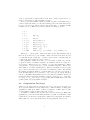
MCheck has no GUI interface but is still simple to use. The command mch
test.txt will verify the LTL and CTL formulas given in test.txt for the model
given in test.txt. A model is given by writing for each state the name followed
by the states to which the state has transitions and the propositions that are
true in the state. The initial state is indicated with ‘>’ before the name of the
state. Figure 1 gives an example of how models are represented in MCheck. The
LTL and CTL formulas are written as expected, where the temporal operators
are given with capital letters.
6
{p, q}
{¬p, q}
q0
q1
q3
q2
{p, ¬q}
{¬p, ¬q}
{>0
1
2
3
}
0 1 2
1 2
3
3 0
p q
q
p
Figure 1: How a model is represented in MCheck
3.2
Mocha
There are two versions of Mocha, cMocha [2] and jMocha [1]. cMocha is the
first version and is mostly written in C. jMocha is the second version and is
mostly written in Java. On Windows jMocha didn’t fully work, on Linux it did,
cMocha didn’t work at all1 .
jMocha can only do invariant and refinement checking. Invariant checking
can only check formulas of the form ⟪A⟫◻ϕ where ϕ doesn’t contain any other
temporal operators. Nesting temporal operators is not possible. Refinement
checking is checking whether the traces generated by one model is a subset of
the traces generated by another model.
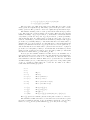
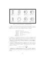
Giving a model to Mocha is not as simple as it is in MCheck. A set of
variables is given instead of a set of states. Each possible combination of values
of the variables is a state. The transitions between the states are given by
allowing each player to only change certain variables. Each variable can only
be controlled by one player. The strategy of the player is given by formulas
that assign values to the variables. These formulas can use variables controlled
by other players. Every game structure can be represented in this way, but
the translation isn’t always straightforward. Figure 2 gives an example of how
models are represented in Mocha.
1 Installing cMocha on Linux gave the following problems. tcl version 8.6 doesn’t work
with Tix version 8.4.3. The code in until.h has (obj)=0 instead of (obj)==0 (line 175 and
185). File invMain.c gives and error (line 127). The file configure of mocha-1.0.1 has an
apostrophe to much (line 850). File prsLex.c gives an error (line 1527).
7
B
A
{p, q}
{¬p, q}
q0
A
q1
B
q3
B
A
q2
{p, ¬q}
{¬p, ¬q}
A
B
module A is
interface p : bool
external q : bool
atom contp controls p reads q
init
[] true -> p’ := true
update
[] q -> p’ := false
[] ~q -> p’ := true
module B is
interface q : bool
external p : bool
atom contq controls q reads p
init
[] true -> q’ := true
update
[] p -> q’ := false
[] ~p -> q’ := true
Figure 2: How a model is represented in Mocha
8
4
Spatial reasoning
Now that we have defined LTL, CTL and ATL and described model checkers
for these temporal logics we want to represent spatial information with these
temporal logics. Every temporal step between states can be seen as a step
in spatial space. What can be expressed with the temporal logics is however
not very useful for spatial reasoning. That is why we represent RCC with the
temporal logics. First we will define RCC and then we try to represent it with
the temporal logics.
4.1
Region Connection Calculus
RCC is a way to represent relations between regions. The definition for RCC
is based on the C(X, Y ) relation which means X connects with Y [9]. Where
X and Y are spatial regions. This relation is reflexive and symmetric, thus X
is connected with itself and if X is connected with Y then is Y connected with
X. All other relations are defined with C(x, y) in the following way:
DC(X, Y ) ∶= ¬C(X, Y )
P(X, Y ) ∶= ∀Z [C(Z, X) → C(Z, Y )]
PP(X, Y ) ∶= P(X, Y ) ∧ ¬P(Y, X)
EQ(X, Y ) ∶= P(X, Y ) ∧ P(Y, X)
O(X, Y ) ∶= ∃Z [P(Z, X) ∧ P(Z, Y )]
PO(X, Y ) ∶= O(X, Y ) ∧ ¬P(X, Y ) ∧ ¬P(Y, X)
DR(X, Y ) ∶= ¬O(X, Y )
TPP(X, Y ) ∶= PP(X, Y ) ∧ ∃Z [EC(Z, X) ∧ EC(Z, Y )]
EC(X, Y ) ∶= C(x, y) ∧ ¬O(X, Y )
NTPP(X, Y ) ∶= PP(X, Y ) ∧ ¬∃Z [EC(Z, X) ∧ EC(Z, Y )]
P−1 (X, Y ) ∶= P(Y, X)
PP−1 (X, Y ) ∶= PP(Y, X)
TPP−1 (X, Y ) ∶= TPP(Y, X)
NTPP−1 (X, Y ) ∶= NTPP(Y, X)
DC(X, Y ) stands for X is disconnected from Y , P(X, Y ) stands for X is
part of Y , PP(X, Y ) stands for X is a proper part of Y , EQ(X, Y )2 stands for
X is equivalent to Y , O(X, Y ) stands for X overlaps Y , PO(X, Y ) stands for
X partially overlaps Y , DR(X, Y ) stands for X is discrete from Y , TPP(X, Y )
stands for X is a tangential proper part of Y , EC(X, Y ) stands for X is externally
connected with Y , NTPP(X, Y ) stands for X is a non-tangential proper part of
Y . For the inverse of φ the notation φ−1 is used, where φ ∈ {P, PP, TPP, NTPP}.
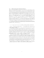
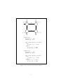
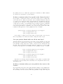
In this article we will use RCC8. RCC8 only uses the relations DC, EC,
PO, EQ, TPP, NTTP, TTP−1 and NTTP−1 . A visual representation of these
relations is shown in Figure 3.
2 In
[9] X = Y is used instead of EQ(X, Y ).
9
X
X
Y
Y
DC(X, Y )
PO(X, Y )
X
Y
TPP(X, Y )
Y
X
TPP−1 (X, Y )
X
X Y
X
Y
Y
X
Y
EC(X, Y )
EQ(X, Y )
NTPP(X, Y )
NTPP−1 (X, Y )
Figure 3: A visual representation of the RCC8 relations
There is a distinction between the interior and the boundary of a region.
The interior of ϕ is denoted iϕ. Looking at Figure 3 it is easy to see that the
RCC8 relations can also be defined with the following set formulas:
DC(X, Y ) ∶= X ∩ Y = ∅
EC(X, Y ) ∶= X ∩ Y =/ ∅ ∧ iX ∩ iY = ∅
PO(X, Y ) ∶= X ⊆/ Y ∧ Y ⊆/ X ∧ iX ∪ iY =/ ∅
EQ(X, Y ) ∶= X = Y
TPP(X, Y ) ∶= X ⊂ Y ∧ X ⊂/ iY
NTPP(X, Y ) ∶= X ⊂ iY
Modal Logics for Qualitative Spatial Reasoning [5] gives a translation from
RCC constraints to multimodal propositional logic. We want a translation from
RCC constraints to LTL, CTL and ATL. On the Translation of Qualitative Spatial Reasoning Problems into Modal Logics [7] gives a proof for the translation
to multimodal propositional logic. I’m using a similar proof for the translation
to the temporal logics.
We give a formal language called set expression. It is easier to use set
expressions for our purposes then the set formulas given above. Set expressions
s and t are with the following grammar. X, Y and Z denote the countable
infinite set of variables.
s, t ∶∶= X ∣ ⊺ ∣ – ∣ s ⊔ t ∣ s ⊓ t ∣ s ∣ Is
Elementary set constraints have the form s ≐ t or s ≐/ t. More complex set
constraints can be constructed using the propositional connectives conjunction,
disjunction and negation. If S and T are set constraints then so are S ∧ T , S ∨ T
and ¬S.
10
The function d maps every set expression to a subset of a topological space.
A topological space consist of a universe U and a set i of subset of U . d maps
every set expression to a subset of U in the following way:
d(–) = ∅
d(⊺) = U
d(s ⊓ t) = d(s) ∩ d(t)
d(s ⊔ t) = d(s) ∪ d(t)
d(s) = U / d(s)
d(Is) = i(d(s))
A topological interpretation I is a triple I = (U, i, d). We write I ⊧ C if
topological interpretation I satisfies a set constraint C. The topological interpretation for elementary constraints is defined as below. The conjunction,
disjunction and negation in complex topological interpretations are defined in
their usual way.
I ⊧ s ≐ t iff d(s) = d(s)
I ⊧ s ≐/ t iff d(s) ≠ d(s)
Now we can rewrite the RCC relations from set formulas into the set expressions:
DC(X, Y ) ∶= X ⊓ Y ≐ –
EC(X, Y ) ∶= X ⊓ Y ≐/ – ∧ IX ⊓ IY ≐ –
PO(X, Y ) ∶= IX ⊓ IY ≐/ – ∧ X ⊓ Y ≐/ – ∧ X ⊓ Y ≐/ –
EQ(X, Y ) ∶= X ≐ Y
TPP(X, Y ) ∶= X ⊓ Y ≐ – ∧ X ⊓ IY ≐/ ⊥
NTPP(X, Y ) ∶= X ⊓ IY ≐ –
The temporal logics LTL, CTL and ATL are not continues, they are based
on transitions systems. This means that the spatial regions used in RCC must
also be represented in a transition system Ts = (Q, q0 , δ, Π, l) that we call spatial
transition system. The universe U will be the set of all states Q. q0 is a state
that’s not part of any region. δ is the reachability between states. typically, if
two states are next to each other in the spatial space then they are connected in
both ways. A region will be a set of states where a certain proposition is true.
The distinction between the interior and the boundary of a region is made with
the reachability of states. The interior has no transitions to states outside the
interior. This makes it possible to say that something holds inside the interior
of are region with the expression it holds in all reachable states, starting inside
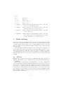
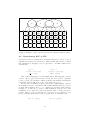
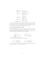
the region. Figure 4 gives an example of a spatial transition system. Dotted
lines show which part of the transition system corresponds to the regions. The
set of true propositions are given for each state. The regions are represented in
a five by nine grid of states. Typically a lot more states are used, but for the
clarity of this example we used the minimal number of states necessary. It is
also not required for the states to be in a grid.
11
X
Y
Z
{X}
{X}
{X,Y} {Y}
{Y,Z}
{Y,Z}
{Y,Z}
{Z}
{Z}
{X}
{X}
{X,Y} {Y}
{Y,Z}
{Y,Z}
{Y,Z}
{Z}
{Z}
{X}
{X}
{X,Y} {Y}
{Y,Z}
{Y,Z}
{Y,Z}
{Z}
{Z}
Figure 4: Example of three regions represented in a spatial transition system
4.2
Representing RCC in LTL
Now that we have set expressions for the RCC8 relations we can try to give a
translation from these set expressions to LTL formulas. The function α makes
this translation by mapping every set expression to an LTL formula in the
following way:
α(–) = –
α(⊺) = ⊺
α(s ⊓ t) = α(s) ∧ σ(t)
α(s ⊔ t) = α(s) ∨ α(t)
α(s) = ¬α(s)
α(Is) = ◻α(s)
Most of these mappings are very straightforward. The mapping of the S4
operator α(Is) to ◻α(s) isn’t directly obvious. I is a S4 operator, equivalent
to the ◻ operator in a S4 frame. LTL is a reflexive and transitive and thus has
a S4 frame. Because LTL is S4, α(Is) can be mapped to ◻α(s).
We now have a translation from set expressions to LTL formulas. However
the translation from set constraints to LTL formulas with the functions α gives a
problem. The translation from s ≐ ⊺ to s must hold everywhere in the universe
is simple to do with the ◻ operator. This translation is given below. But
translating s ≐/ ⊺ to there is a point in the universe where s doesn’t hold is not
possible. The ◇ operator seems like a good option, but ◇ϕ means on every
path ϕ eventually holds and not there is a path where ϕ eventually holds.
α(s ≐ ⊺) = ◻α(s)
α(s ≐ –) = ◻¬α(s)
12
We can only translate set constraints where ≐/ is not used. Only the RCC set
expressions DC, EQ and NTPP don’t use ≐/ . Using the set expressions of these
RCC relations gives the following result:
α(DC(X, Y )) = ◻¬(X ∧ Y )
α(EQ(X, Y )) = ◻(¬X ∨ Y ) ∧
◻(X ∨ ¬Y )
α(NTPP(X, Y )) = ◻(¬X ∨ ◻Y )
LTL can only represent the RCC relations DC, EQ and NTPP and not all
RCC8 relations. This is because in LTL the formulas must hold for all paths.
A formula that holds for some paths cannot be represented in LTL but can be
represented in CTL.
4.3
Representing RCC in CTL
We will show that in CTL you can represent RCC. The proof is similar to the
one given for LTL, but now we can represent formulas that hold for some paths.
The function β maps every set expression formula to a CTL formula in the
following way:
β(–) = –
β(⊺) = ⊺
β(s ⊓ t) = β(s) ∧ β(t)
β(s ⊔ t) = β(s) ∨ β(t)
β(s) = ¬β(s)
β(Is) = ∀◻β(s)
Just like with LTL the S4 operator Is is translated with the ◻ operator. It
is translated to ∀◻β(s) because s must hold everywhere in the region. Because
there are no transitions from the interior of a region to the outside s must always
hold on all paths.
In CTL we can represent set constraints in the following way:
β(s ≐ ⊺) = ∀◻β(s)
β(s ≐ –) = ∀◻¬β(s)
β(s ≐/ ⊺) = ∃◇¬β(s)
β(s ≐/ –) = ∃◇β(s)
Using β on the RCC set expressions gives the following result:
13
β(DC(X, Y )) = ∀◻¬(X ∧ Y )
β(EC(X, Y )) = ∀◻¬(∀◻X ∧ ∀◻Y ) ∧
∃◇(X ∧ Y )
β(PO(X, Y )) = ∃◇(∀◻X ∧ ∀◻Y ) ∧
∃◇(X ∧ ¬Y ) ∧
∃◇(¬X ∧ Y )
β(EQ(X, Y )) = ∀◻(¬X ∨ Y ) ∧
∀◻(X ∨ ¬Y )
β(TPP(X, Y )) = ∀◻(¬X ∨ Y ) ∧
∃◇(X ∧ ¬∀◻Y )
β(NTPP(X, Y )) = ∀◻(¬X ∨ ∀◻Y )
We now have a representation of RCC8 in CTL. However the representation
of regions in the transition system makes temporal reasoning not possible. There
is no distinction between temporal transitions and spatial transitions. We need
to make a distinction between temporal and spatial operators.
4.4
Representing RCC in ATL
Just like in CTL, RCC can be represented in ATL. But we can make a distinction
between temporal and spatial operators by making a distinction between players
for temporal reasoning and players for spatial reasoning. γ maps every set
expression formula to an ATL formula in the following way:
γ(–) = –
γ(⊺) = ⊺
γ(s ⊓ t) = γ(s) ∧ γ(t)
γ(s ⊔ t) = γ(s) ∨ γ(t)
γ(s) = ¬γ(s)
γ(Is) = ⟪As ⟫◻γ(s)
As is the set of players active in s.
Set constraints are represented in the following way:
γ(s ≐ ⊺) = ⟪As ⟫◻γ(s)
γ(s ≐ –) = ⟪As ⟫◻¬γ(s)
γ(s ≐/ ⊺) = ⟪As ⟫◇¬γ(s)
γ(s ≐/ –) = ⟪As ⟫◇γ(s)
Using γ on the RCC set expressions gives the following result, where region
X is defined by player x and region Y by player y.
14
γ(DC(X, Y )) = ⟪x, y⟫◻¬(X ∧ Y )
γ(EC(X, Y )) = ⟪x, y⟫◻¬(⟪x⟫◻X ∧ ⟪y⟫◻Y ) ∧
⟪x, y⟫◇(X ∧ Y )
γ(PO(X, Y )) = ⟪x, y⟫◇(⟪x⟫◻X ∧ ⟪y⟫◻Y ) ∧
⟪x, y⟫◇(X ∧ ¬Y ) ∧
⟪x, y⟫◇(¬X ∧ Y )
γ(EQ(X, Y )) = ⟪x, y⟫◻(¬X ∨ Y ) ∧
⟪x, y⟫◻(X ∨ ¬Y )
γ(TPP(X, Y )) = ⟪x, y⟫◻(¬X ∨ Y ) ∧
⟪x, y⟫◇(X ∧ ¬⟪y⟫◻Y )
γ(NTPP(X, Y )) = ⟪x, y⟫◻(¬X ∨ ⟪y⟫◻Y )
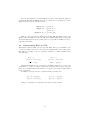
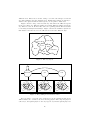
Making a distinction between temporal players and spatial players makes
it possible to represent both temporal and spatial information in a transition
system. Figure 5 gives an example of how this is done. Every node in the temporal transition system is replaced with the set of nodes of the spatial transition
system. These nodes are connected for the spatial player. In the example these
are q0 , q1 and q2 . All these nodes are connected for the temporal player with
the node on the same location in the next state. In the example a few of these
connections are represented by dotted lines.
qo
q1
◯◯Y
q2
◯Y
◇X
Y
X
Figure 5: The representation of three temporal states in ATL
5
Parking example
In this example we show how the combination of ATL and RCC can be used to
reason about parking fees. There are often different parking zones in a city with
15
different rates. These rates can also change over time. We will give a fictional
city with parking zones and changing rates. Within this example we will try to
answer some questions like in what regions you can park for what rates.
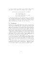
Figure 6 shows a map of the fictional city and names the different regions
in the city. There are different parking zones with different parking fees in the
city. There is a rate A, B and C. We denote free parking with 0. The rates differ
for weekday, Saturdays and Sunday’s. Figure 7 shows the transition system for
this situation and the rates for the different zones and the different days.
North West North East
Centre
East
West
South East
South
Figure 6: The city layout
Mon-Fri
Sat
0
B
0
A
B
Sun
0
B
C
C
0
0
B
0
C
0
0
B
0
0
B
C
0
0
0
Figure 7: The parking zones and there rates
We now want to represent some questions about the parking in this city in
ATL formula’s. To do this we use the following players. The temporal player is
called days, the spatial player for the city regions city and the spatial player for
16
the parking zones zone. When the questions are translated to ATL formula’s
we can use a model checker to get the answer.
Is there a moment when I can park in the Centre for free?
It is possible to park in the Centre for free if the Centre region overlaps with
a zone with rate 0. “There is a moment” can be translated with the temporal
◇ operator. Note that if we want to know whether we can park in a region for
a certain rate we only have to check whether the region and the zone partially
overlap. We don’t have to check whether the zone and the region are equivalent
or are some proper part of each other, because in this example there are no
zones and regions that are equivalent or are a proper part of each other. The
formula for this question becomes ◇PO(Centre, 0), or in ATL:
⟪days⟫◇(⟪city, zone⟫◇(⟪city⟫◻Centre ∧ ⟪zone⟫◻0) ∧
⟪city, zone⟫◇(Centre ∧ ¬0) ∧
⟪city, zone⟫◇(¬Centre ∧ 0))
It is possible to park for free in the Centre at any moment. On every day
there is a parking fee for all the zones that overlap the Centre region.
Can you park in South with rate B for two days?
Just like with the previous question, if we want to know whether we can park
in a region for a certain rate we only have to check whether the region and the
zone partially overlap. But now we want to check it for the current state and
the next. We can check the next state using the temporal ◯ operator. The
formula for this question becomes PO(South, B) ∧ ◯PO(South, B), or in ATL:
(⟪city, zone⟫◇(⟪city⟫◻South ∧ ⟪zone⟫◻B) ∧
⟪city, zone⟫◇(South ∧ ¬B) ∧
⟪city, zone⟫◇(¬South ∧ B)) ∧
(⟪days⟫◯⟪city, zone⟫◇(⟪city⟫◻South ∧ ⟪zone⟫◻B) ∧
⟪city, zone⟫◇(South ∧ ¬B) ∧
⟪city, zone⟫◇(¬South ∧ B)))
We start on a weekday, as shown in Figure 7. It is possible to park in South
for rate B on every weekday and on Saturday. You can park in South for two
days with rate B.
Is there a moment when you can park for free next to the
Centre?
If you can park for free next to the Centre then there must be a free parking zone
just outside of the Centre region. This is the case when the region and the zone
are externally connected, but also when they partially overlap. The temporal
17
◇ operator is again used for translating “there is a moment”. The formula for
this question becomes ◇(EC(Centre, 0) ∨ PO(Centre, 0)), or in ATL:
⟪days⟫◇((⟪city, zone⟫◇(⟪city⟫◻Centre ∧ ⟪zone⟫◻0) ∧
⟪city, zone⟫◇(Centre ∧ ¬0) ∧
⟪city, zone⟫◇(¬Centre ∧ 0)) ∨
(⟪city, zone⟫◻¬(⟪city⟫◻Center ∧ ⟪zone⟫◻0) ∧
⟪city, zone⟫◇(Centre ∧ 0)))
We already know that you can never park in the Centre for free. Meaning
there is no partial overlap between the centre and a free parking zone. But there
is a moment when the Centre and a free parking zone are externally connected.
Namely on Sunday you can park for free just east and just west of the Centre.
There is a moment when you can park for free next to the Centre.
6
Conclusion
In this article we asked whether RCC relations could be represented into a
temporal logic and whether this could be done in such a way that the spatial
regions and the temporal relations can be used like in a spatio-temporal logic.
We have found that LTL can only represent the RCC relations DC, EQ and
NTPP. We found that CTL can represent all the RCC relations, but it is not
possible to also use temporal relations. We found that in ATL both the spatial
RCC relations and temporal relations can be used like in a spatio-temporal logic.
This is possible by making a distinction between temporal and spatial players.
We wanted to represent a spatial logic into a temporal logic so that the
existing model checker for the temporal logic could be used. However there is
only one model checker for ATL we are aware of and it’s difficult to use and
install. There are a lot more model checkers for LTL and CTL available. A
model checker for CTL could be used to check RCC models.
Because the model checker for ATL is difficult to use it might be better to
develop a spatio-temporal model checker instead of using an existing temporal
model checker. In this article we only discussed RCC as the spatial logic. Future
research could focus on representing other spatial logics into temporal logics.
Future research could also focus on other temporal logics to represent the spatial
logics.
In artificial intelligence temporal logics is used to reason about time and
spatial logics to reason about space. In this article we combined some of these
temporal and spatial logics into a spatio-temporal logic. Making it possible to
reason about space changing over time, like in the given parking example.
18
References
[1] R Alur, H Anand, F Ivancić, M Kang, M McDougall, BY Wang, L de Alfaro, TA Henzinger, B Horowitz, R Majumdar, FYC Mang, C MeyerKrisch, M Minea, S Qadeer, SK Rajamani, and JF Raskin. MOCHA user
manual. Jmocha version 2.0.
[2] R Alur, L De Alfaro, Th A Henzinger, SC Krishnan, FYC Mang, S Qadeer,
SK Rajamani, and S Tasiran. MOCHA user manual.
[3] Rajeev Alur, Thomas A Henzinger, and Orna Kupferman. Alternating-time
temporal logic. Journal of the ACM (JACM), 49(5):672–713, 2002.
[4] Christel Baier, Joost-Pieter Katoen, et al. Principles of model checking,
volume 26202649. MIT press Cambridge, 2008.
[5] Brandon Bennett. Modal logics for qualitative spatial reasoning. Logic
Journal of IGPL, 4(1):23–45, 1996.
[6] Roman Kontchakov, Agi Kurucz, Frank Wolter, and Michael Zakharyaschev. Spatial logic+ temporal logic=? In Handbook of spatial
logics, pages 497–564. Springer, 2007.
[7] Werner Nutt. On the translation of qualitative spatial reasoning problems
into modal logics. In KI-99: Advances in Artificial Intelligence, pages 113–
124. Springer, 1999.
[8] Amir Pnueli. The temporal logic of programs. In Foundations of Computer
Science, 1977., 18th Annual Symposium on, pages 46–57. IEEE, 1977.
[9] David A Randell, Zhan Cui, and Anthony G Cohn. A spatial logic based
on regions and connection. KR, 92:165–176, 1992.
[10] Jeff Sember. Mcheck: A model checker for ltl and ctl formulas. 2005.
19