Download as a PDF

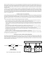
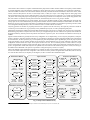
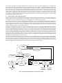
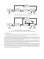
In Proceedings of International Symposium on Intelligent Robotics (ISIR ‘93)
Bangalore, India, January 1993..
Integration of Real-Time Software Modules for
Reconfigurable Sensor-Based Control Systems
David B. Stewart†, Richard A. Volpe‡, Pradeep K. Khosla†
†
Department of Electrical and Computer Engineering and The Robotics Institute
Carnegie Mellon University, Pittsburgh, PA 15213
‡
The Jet Propulsion Laboratory, California Institute of Technology
4800 Oak Grove Drive, Pasadena, California 91109.
Abstract—In this paper we develop a framework for integrating real-time software modules that comprise a reconfigurable multisensor based system. Our framework is based on the proposed concept of a global database of state information through which realtime software modules exchange information. This methodology allows the development and integration of reusable software in a
complex multiprocessing environment. A reconfigurable sensor-based control system consists of many software modules, each of
which can be modelled using a simplified version of a port automaton. Our new state variable table mechanism can be used in both
statically and dynamically reconfigurable systems, and it is completely processor independent. Individual modules may also be
combined into larger modules to aid in building large systems, and to reduce bus and CPU utilization. An efficient implementation
of the state variable table mechanism, which has been integrated into the Chimera II Real-Time Operating System, is also described.1
Keywords—reconfigurable sensor-based control systems, reusable software, real-time operating systems, interprocessor communication, spin-locks, real-time software modelling.
I. INTRODUCTION
Real-time sensor based control systems are complex. In order to develop such systems, control strategies are needed to interpret and process
sensing information for generating control signals. There has been considerable effort devoted to addressing this aspect of real-time control
systems. However, even with robust control algorithms, a sophisticated software environment is necessary for efficient implementation into
a robust system. The level of sophistication is even greater if this system is to be generalized so that it is reconfigurable and can perform
more than a single task or application. Obviously, a real-time operating system (RTOS) is part of this software environment. However, it is
also necessary to have a layer of abstraction between the RTOS and control algorithms that makes the implementation efficient, allows for
easily expanding and/or changing the control strategies, and reduces development costs by incorporating the concept of reusable software.
The development of this layer of abstraction is further motivated by the realization that real-time control systems are typically implemented
in open-architecture multiprocessor environments. Several issues, such as configuring reusable modules to perform a job, allocating modules to processors, communicating between various modules, synchronizing modules running on separate processors, and determining correctness of a configuration, arise in this context.
In this paper we develop a framework for integrating real-time software modules that comprise a reconfigurable multi-sensor based system.
Our framework is based on the proposed concept of a global database of state information through which real-time software modules exchange information. This methodology allows the development and integration of reusable software in a complex multiprocessing environment.
We define a control module as a reusable software module within a real-time sensor-based control subsystem. A reconfigurable system consists of many control modules, each of which can be modelled using a simplified version of a port automaton [22], as shown in Fig. 1. Each
module has zero or more input ports, and zero or more output ports. Each port corresponds to a data item required or generated by the control
module. A module which obtains data from sensors may not have any input ports, while a module which sends new data to actuators may
not have any output ports. We assume that each control module is a separate task2. A control module can also interface with other subsystems, such as vision systems, path-planners, or expert systems.
A link between two modules is created by connecting an output port of one module to an appropriate input of another module. A legal configuration is obtained if for every input port in the system, there is one, and only one, output port connected to it. An extension of the port
automata theory is presented in [12], where a split connector allows a single output to be fanned into multiple output ports, and a join connector allows multiple input ports to be merged into a single input port. The split connector replicates the output multiple times. For the join
connector, a combining algorithm, such as a weighted average, is required to merge the data.
1. The research reported in this paper is supported, in part by, U.S. Army AMCOM and DARPA under contract DAAA-2189-C-0001, the National Aeronautics and Space
Administration (NASA), the Department of Electrical and Computer Engineering, and by The Robotics Institute at Carnegie Mellon University. Partial support for David B. Stewart
is provided by the Natural Sciences and Engineering Research Council of Canada (NSERC) through a Graduate Scholarship. The research reported in this paper was also performed,
in part, for the Jet Propulsion Laboratory (JPL), California Institute of Technology, for the Remote Surface Inspection system development and accompanying projects [26] under
a contract with NASA. Reference herein to any specific commercial product, process, or service by trade name, trademark, manufacturer, or otherwise, does not constitute or imply
its endorsement by the United States Government or JPL.
2. We define a task as a separate thread of control within a multitasking operating system. The definition is consistent with that of the Chimera II Real-Time Operating System
[23], and is also known as a thread in Mach and POSIX, and a lightweight process in some other operating systems.
Other environments developed for robot control ([1][2][3][5][14]) lack the flexibility required for the design and implementation of reconfigurable systems. The design of these programming environments is generally based on heuristics rather than on software architecture models, and lends itself only to single-configuration systems. The environments also do not make clear distinctions between module interfaces
and module content, thus lacking a concrete framework which would allow development of modules independent of the target application
and target hardware.
In this paper, we propose a method of using state variables for systematically integrating reusable control modules in a real-time multiprocessor environment. Our design can be used with both statically and dynamically reconfigurable systems. Section II describes the design
issues to be considered, and some of the assumptions we have made about the target environment. Section III gives the architectural details
of our control module integration. Section IV describes an efficient implementation of the state variable table mechanism, which has been
integrated into the Chimera II Real-Time Operating System [23]. Finally, Section V summarizes the use of state variables for module integration in a reconfigurable system.
II. DESIGN ISSUES AND ASSUMPTIONS
In order to design a general mechanism which can be used to integrate control modules in a multiprocessor environment, some architectural
knowledge of the target hardware is required. We assume an open-architecture multiprocessor system, which contains multiple general purpose processors (such as MC68030, Intel 80386, SPARC, etc.), which we call Real-Time Processing Units (RTPUs), on a common bus (such
as VMEbus, Multibus, Futurebus, etc.). Each processor has its own local memory, and some memory in the system is shared by all processors.
Given an open-architecture target environment, the following issues must be considered:
Processor transparency: In order for a software module to be reusable, it must be designed and written independent of the RTPU on
which it will finally execute, since neither the hardware nor software configuration is known apriori.
Task synchronization: Sensors and actuators may be operating at different rates, thereby requiring different tasks to have different frequencies. In addition, system clocks on multiple processors may not be operating at the exact same rate, causing two tasks with the
same frequency to have skewing problems. The module integration must not depend on task frequencies or system clocks for synchronization.
Data integrity: When two modules communicate with each other, a complete set of data must be transferred. It is not acceptable for
part of a data set to be from the current cycle, while the rest of the data set is from a previous cycle.
Predictability: In real-time systems, it is essential that the communication between modules is predictable, so that worst-case execution
and blocking times can be bounded. These times are required for analysis by most real-time scheduling algorithms.
Bus bandwidth: In an open-architecture system, a common bus is shared by all RTPUs. The communication between modules must be
designed to minimize the bus traffic.
implementation efficiency: The design must lead to an efficient implementation. Communication mechanisms which incur large
amounts of overhead are not suitable for the high frequency tasks, and therefore cannot be used.
To address these issues, we propose a state variable table mechanism which allows the integration and reconfiguration of reusable modules
in a multiprocessor, open-architecture system.
III. DESIGN OF STATE VARIABLE TABLE MECHANISM
The structure of our state variable table mechanism is shown in Fig. 2. It is based on using global shared memory for the exchange of data
between modules, thus providing communication with minimal overhead. A global state variable table is stored in the shared memory. The
variables in the global state variable table are a union of all the input port and output port variables of the modules that may be configured
into the system. Tasks corresponding to each control module cannot access this table directly. Rather, every task has its own local copy of
the table, called the local state variable table.
Global State Variable Table
x
input ports 1
xn
:
control
module
:
y1
output ports
ym
communication with
sensors, actuators,
and other subsystems
local state
variable table
local state
variable table
local state
variable table
local state
variable table
task
module
A1
task
module
Aj
task
module
K1
task
module
Kj
Processor A
Fig. 1: Port automaton model of a control module
Processor K
Fig. 2: Structure of state variable table mechanism
for control module integration
Only the variables used by the task are kept up-to-date in the local table. No synchronization is needed to access this table, since only a
single task has access to it. At the beginning of every cycle of a task, the variables which are input ports are transferred into the local table
from the global table. At the end of the task’s cycle, variables which are output ports are copied from the local table into the global table.
This design ensures that data is always transferred as a complete set.
When using the global state variable table for inter-module communication, the number of transfers per second3 (Zj) for module Mj can be
calculated as follows:
nj
mj


 ∑ S ( x ij ) + ∑ S ( y ij ) + ∆ 


i=1
i=1
Z j = ------------------------------------------------------------------------Tj
(1)
where nj is the number of input ports for Mj, mj is the number of output ports for Mj, xij is input variable xi for Mj, yij is output variable yi
for Mj, S(x) is the transfer size of variable x, Tj is the period of Mj, and ∆ is the overhead required for locking and releasing the state variable
table during each cycle.
We assume that the entire global state variable has a single lock. It is possible for each variable to have its own lock, in which case the
locking overhead increases to (m+n)∆. The advantage of using a single lock is described in Section .A..
The bus utilization B for k modules in a particular configuration, in transfers per second, is then
k
B =
∑ Zj
(2)
j=1
Thus using our state variable table design, we can accurately determine the CPU and bus utilization required for the inter-module communication within a configuration.
A configuration is legal if the following holds true:
 k, m j
   k, n j
  k, m j

 ∩ y ij = ∅  ∧   ∪ x ij  ⊆  ∪ y ij  
 j = 1, i = 1
   j = 1, i = 1   j = 1, i = 1  
(3)
The first term represents the intersection of all output variables from all modules. If two modules have the same outputs, then a join connector is required. Modules with conflicting outputs can modify their output port variables, such that they are two separate, intermediate
variables. A join connector is a separate module which performs some kind of combining operation, such as a weighted average. Its input
ports are the intermediate variables, while its single output port is the output variable that was originally in conflict. The bandwidth required
can then be calculated by treating the join connector as a regular module. Split connectors are not required in our design, since multiple
tasks can specify the same input port, in which case data is obtained from the same location within the global state variable table. The second
term in (3) states that for every input port, there must be a module with a corresponding output port.
Using state variables for module integration is processor independent. Whether multiple modules run on the same RTPU, or each module
runs on a separate RTPU, the maximum bus bandwidth required for a particular configuration remains constant, as computed in (2). In the
next section we give more details on typical modules within a reconfigurable sensor-based control system.
A. Control Module Library
The state variable table mechanism is a means of integrating control modules, which have been developed with a reusable and reconfigurable interface. Once a module is developed, it can be placed into a library, and incorporated into a user’s application as needed. A sample
control module library is shown in Fig. 3. The classification of different module types is for convenience only. There is no difference in the
interfaces of say, a robot interface module and a digital controller module. We expect that existing robot control libraries (e.g. [2][10]), can
be repackaged into reusable modules in order to use them in reconfigurable systems.
The following variable notation is used:
The following subscript notation is used:
d: desired (as input by user or path planner)
θ : joint position
x : Cartesian position
r: reference (computed value, commanded on each cycle)
θ̇ : joint velocity
ẋ : Cartesian velocity
m: measured (obtained from sensors on each cycle)
θ̇˙ : joint acceleration
ẋ˙: Cartesian acceleration
f: Cartesian force/torque
y: wild-card: match any subscript
τ : joint torque
u: control signal
J: Jacobian
z: wild-card: match any variable
Robot interface modules communicate directly with robotic hardware. In general a robot is controlled by sending joint torques to an appropriate input/output port, as represented by the torque-mode robot interface module. The current joint position and joint velocity of the robot
can also be retrieved from the hardware interface. With some robots, direct communication with the robot actuator is not possible. The robot
provides its own controller, to which reference joint positions must be sent. The position-mode robot interface is a module for this type of
3. We use “transfers per second” instead of CPU execution time or bus utilization time as a base measure for the resource requirements of the communication mechanism,
since it is a hardware independent measurement.
robot interface. Other actuators or computer controlled machinery may also have similar interface modules. The frequency of these modules
is generally dependent on the robot hardware; sometimes it is fixed, other times it may be set depending on the application requirements.
The sensor modules are similar to the robot interface modules, in that they communicate with device hardware, such as force sensors, tactile
sensors, and vision subsystems. In the case of a force/torque sensor, a 6-DOF force/torque sensor module inputs raw strain gauge values
and converts them into an array of force and torque values, in Newtons and Newton-meters respectively.4 For a visual servoing application
[18], much of the reading and preprocessing of images is performed by specialized vision subsystems. These systems may generate some
data, from which a new desired Cartesian position is derived, as illustrated by the visual servoing interface module.
The teleoperation input modules are also sensor modules. They have been classified separately in order to distinguish user input from other
sensory input. In our control module library the teleoperation modules read from a 6 DOF trackball, thus both modules are similar. The
difference is the type of preprocessing performed by each module, allowing the trackball to be used either for generating velocities (which
can be integrated to obtain positions), or force, for when the robot is in contact with the environment.
Trajectory generators are another way of getting desired forces or positions into the control loop. The input may come from outside the
control loop, such as from the user (e.g. keyboard), from a predefined trajectory file, or from a path-planning subsystem.
Differentiator and integrator modules perform time differential and integrals respectively. For example, joint velocities may be obtained by
differentiating joint positions. Only the value of the current cycle is supplied as input. Previous values are not required, as the modules are
designed with memory, and keep track of the positions and velocities of previous cycles. The current time is assumed to be known by all
modules.
Digital controller modules are generally the heart of any configuration. In our sample library, we have trajectory interpolators, a PID joint
position controller, a resolved acceleration controller [11], an impedance controller [6], and other supporting modules such as forward and
inverse kinematics, Jacobian operations [19], inverse dynamics [8], and a damped least squares algorithm [29]. Given the proper input and
output port matching, various controller modules can be integrated to perform different types of control. Sometimes a particular control
configuration will not need all of its inputs. Those inputs are often set to zero. The zero module provides a constant value 0 to an input
stream. Theoretically this would be a single task which always copies the constant variable to the global state variable table. However, in
practice, the global state variable table only has to be updated once, after which time the module no longer has to execute, thus saving on
both RTPU and bus bandwidth. This practice is equivalent to setting the frequency of task zero to infinity.
Many of the modules require initialization information. For example, the PID controller module requires gains, and the forward kinematics
and Jacobian module requires the robot configuration. These values can also be passed via the global state variable table, and are read only
once from the table. However, for simplicity in our diagrams, we have not shown these initialization inputs.
Robot Interface Modules
τr
torque-mode
robot
interface
θm
xm
θm
xd
θm
from robot:
raw joint
position data
θr
to robot:
raw torque
command
position-mode
robot
interface
θm
θm
θd
Cartesian
trajectory
interpolator
xr
joint pos/vel
trajectory
interpolator
θr
θd
θm
PID joint
position
controller
to robot:
joint move
command
u
Differentiators and Integrators
zy
time
differentiator
zy
xd
xm
time
integrator
zy
inverse
kinematics
θy
u
θm
inverse
dynamics
τr
θm
θm
resolved
acceleration
controller
J
xd
u
xd
xm
xm
xm
xd
J
xd
zy
xy
J
xd
xd
xm
θr
θd
θd
forward
kinematics
and Jacobian
θm
xr
θm
from robot:
raw joint
pos/vel data
Teleoperation Input Modules
Digital Controllers
fm
xm
xm
impedance
controller
u
xr
6-DOF
trackball
x-velocity
J
xd
6-DOF
trackball
force
fd
from trackball:
raw reference data
from trackball:
raw reference data
Trajectory Generators
Jacobian
multiply
trajectory
generator
x-position
xd
θd
xm
from user, file,
or path-planning
subsystem
Jacobian
transpose
trajectory
generator
θ-position
from user, file,
or path-planning
subsystem
τr
Sensor Modules
damped
least squares
θr
zero
0
6-DOF
force/torque
sensor
from f/t sensor
raw strain
gauge data
Fig. 3: Sample Control Module Library
4. For consistency among modules, all input and output variables have units defined by the système internationale (SI).
fm
visual
servoing
interface
from vision
subsystem
xd
xd
Given a library of modules, several legal configurations may be possible. Fig. 4 shows one possible configuration for a teleoperated robot
with a torque-mode interface. Each module is a separate task and can execute on its own RTPU, or multiple modules may share the same
RTPU, without any code modification. The state variable table mechanism allows the frequency of each task to be different. The selection
of frequencies will often be constrained by the available hardware. For example, the robot interface may require that a new torque be supplied every 2 msec cycle time (500 Hz frequency), while the trackball may only supply data every 33.3 msec (30 Hz frequency). Digital
control modules do not directly communicate with hardware, and can execute at any frequency. Generally the frequency for the control
modules will be a multiple of the robot interface frequency. When using the state variable table for communication between the modules,
any combination of frequencies among tasks will work. This allows frequencies to be set as required by the application, as opposed to being
constrained by the communications protocol.
3.2
Reusable Modules and Reconfigurable Systems
The primary goal of the global state variable table mechanism is to integrate reusable control modules in a reconfigurable, multiprocessor
system. The previous section gave examples of control modules, and a sample configuration. In this section, we will give an example of
reconfiguring a system to use a different controller, without changing the sensor and robot interface modules.
Fig. 5 shows two different visual servoing configurations demonstrating the concept of reusable modules. Both configurations obtain a new
desired Cartesian position from a visual servoing subsystem, and supply the robot with new reference joint positions. The configuration in
(a) uses standard inverse kinematics, while the configuration in (b) uses a damped least squares algorithm to prevent the robot from going
through a singularity [29]. The visual servoing, forward kinematics and Jacobian, and position-mode robot interface modules are the same
in both configurations. Only the controller module is different..
The change in configurations can occur either statically or dynamically. In the static case, only the task modules required for a particular
configuration are created. In the dynamic case, the union of all task modules required are created during initialization of the system. Assuming we are starting up using configuration (a), then the inverse kinematics task is turned on immediately after initialization, causing it
to run periodically, while the damped least squares and time integrator tasks remain blocked, or off. At the instant that we want the dynamic
change in controllers, we block the inverse kinematics task and turn on the damped least squares and time integrator tasks. On the next
cycle, the new tasks will automatically update their own local state variable table, and execute a cycle of their loop, instead of the inverse
kinematics task doing so. Assuming the on and off operations are fairly low overhead (which they are in our implementations) the dynamic
reconfiguration can be performed without any loss of cycles. Note that for a configuration to properly execute, the set of modules must be
schedulable on the available RTPUs, as described in [24].
Note that open-ended outputs are fine (e.g. forward kinematics and Jacobian module output port J in (a)) as the module simply generates a
value that is not used. These open-ended outputs generally result when a module must perform intermediate calculations. The intermediate
values can sometimes be used by other modules, and hence they are made available as outputs. The outputs are normally saved in the local
state variable table, and copied to the global table at the end of the cycle. To save on bus bandwidth, these unused outputs do not have to be
updated in the global state variable table, since they are never required as input by the other modules.
xm
θm
Jacobian
multiply
J
forward
kinematics
and Jacobian
xm
θm
xm
resolved
acceleration
controller
xd=0
zero
xd
u
xd
6-dof
trackball
x-velocity
from trackball:
raw reference
data
xd
time
integrator
θm
xd
θm
inverse
dynamics
u
τr
torque-mode
robot
interface
from robot:
raw joint
position data
Fig. 4: Example of module integration: Cartesian teleoperation
θm
θm
to robot:
raw torque
command
xm
forward
kinematics
and Jacobian
J
θm
xm
visual
servoing
interface
Cartesian
trajectory
interpolator
xd
xd
inverse
kinematics
xr
θr
xr
position-mode
robot
interface
from robot:
raw joint
pos/vel data
from vision
subsystem
θm
θm
to robot:
joint move
command
(a) visual servoing using inverse dynamics control module
xm
J
forward
kinematics
and Jacobian
θr
xm
visual
servoing
interface
from vision
subsystem
xd
xd
J
Cartesian
trajectory
interpolator
xr
xr
damped
least squares
θm
time
integrator
θr
position-mode
robot
interface
from robot:
raw joint
pos/vel data
θm
θm
to robot:
joint move
command
(b) visual servoing using damped least squares control module
Fig. 5: Example of system reconfiguration: visual servoing using position-mode robot interface
C. Combining Modules
The model of our control modules allows multiple modules to be combined into a single module. This has two major benefits:
1. complex modules can be built out of smaller, simpler modules, some or all of which may already exist, and hence be reused; and
2. the bus and processor utilization for a particular configuration can be improved.
For maximum flexibility, every component is a separate module, hence a separate task. This structure allows any component to execute on
any processor, and allows the maximum number of different multiprocessor configurations. However, the operating system overhead of
switching between these tasks can be eliminated if each module executes at the same frequency on the same processor. Multiple modules
then make up a single larger module, which can be defined to be a single task.
The bus utilization and execution times for updating and reading the global state variable table may also be reduced. If data from the interconnecting ports of the modules forming the combined modules is not needed by any other module, the global state variable table does not
have to be updated. Since the modules are combined into a single task, they have a single local state variable table. Communication between
those tasks remains local, and thus reduces the bus bandwidth required by the overall application.
The computed torque controller [13] is an example of a combined module. It combines the PID joint position computation module with the
inverse dynamics module, as shown in Fig. 6. The resulting module has the inputs of the PID joint position computation, and the output of
the inverse dynamic module. The intermediate variable u does not have to be updated in the global state variable table. In addition, the measured joint position and velocity is only copied into the local state variable once, since by combining the two modules, both modules use
the same local table. Note that combining modules is only desirable if they can execute at the same frequency on the same RTPU at all times,
as a single module cannot be distributed among multiple RTPUs.
IV. IMPLEMENTATION
We have implemented a state variable table mechanism (which we call svar) and integrated it with the Chimera II Real-Time Operating
System [23]. Our target hardware architecture is a VMEbus-based [17] single-board computers, with multiple MC68030 processor boards.
Functional and syntactic details of the svar mechanism can be found in [25].
First, the global state variable table is created in shared memory. A configuration file which contains the union of all possible state variables
within the system is then read. Once the global state variable table is created, any task can attach to it, at which time a block of local memory
is allocated and initialized for the task. Data for a specific variable can then be transferred between the global and local tables.
In our implementation, we give the ability to transfer multiple variables by preprogramming the list of variables that should be transferred
from the global table at the beginning of a task’s cycle, and to the global table at the end of its cycle. A typical module task would then have
the following format:
call module initialization
preprogram list of input and output variables
begin loop
copy input variables from global table to
local table
execute one cycle of module
copy output variables from local table to
global table
pause until beginning of next cycle
end loop
The preprogram and copy statements are provided by our svar implementation. The pausing and looping are handled by the operating system. Therefore, modules can be defined as subroutine components with a standard interface, which are called at the appropriate time by the
above generic framework.
A. Locking Mechanism
So far we have assumed that tasks can transfer data as needed. However, since the global state variable table must be accessed by tasks on
multiple RTPUs, appropriate synchronization is required to ensure data integrity. A task which is updating the table must first lock it, to
ensure that no other task reads the data while it is changing. Two locking possibilities exist:
1. keep a single lock for the entire table
2. lock each variable separately
The main advantage of the single lock is that locking overhead is minimized. A module with multiple input or output ports only has to lock
the table once before transferring all of its data. There appear to be two main advantages of locking each variable separately: 1) multiple
tasks can read or write different parts of the table simultaneously, and 2) transfers of data for multiple variables by a low priority task can
be preempted by a higher priority task. Closer analysis, however, shows that locking each variable separately does not have these advantages. First, because the bus is shared, only one of multiple tasks holding a per-variable lock can access the table at any one time. Second,
we will show later that the overhead of locking the table, which in effect is the cost of preemption, is often greater than the time for a task
to complete its transfer. A single lock for the entire table is thus recommended.
Next, an appropriate locking mechanism must be selected. Simple mechanisms like local semaphores and only locking the CPU cannot be
used, because they are only valid for single-processor applications. Multiprocessor mechanisms available include spin-locks [15], message
passing, remote semaphores [23], and the multiprocessor priority ceiling protocol [20].
The message passing, remote semaphores, and multiprocessor priority ceiling protocol all require significant overhead, which is typically
an order of magnitude greater than the data transfer itself. For example, the remote semaphores in Chimera II take a minimum of 44 µsec
for the locking and unlocking operations, and as much as 200 µsec if the lock is not obtained on the first try and forces the task to block
[23]. A typical transfer, on the other hand, may consist of 6 joint positions and 6 joint velocities, for a total of 12 transfers. On a typical
VMEbus system, the raw data transfer (i.e. excluding all overhead) takes approximately 16 µsec. The message passing and the multiprocessor priority ceiling protocol would require significantly more overhead than the remote semaphores. It is thus not reasonable to use the
higher level synchronization primitives for locking the state variable table.
The simplest multiprocessor synchronization method is the spin-lock, which uses an atomic test-and-set (TAS) operation. The TAS instruction reads the current lock value from memory, then writes 1 into that location. If the original value is 0, then the task acquires the lock,
otherwise the lock is not obtained, and the task must try again. The read and write portions of the instruction are guaranteed to be atomic,
θd
θd
θd
θm
θm
PID joint
position
controller
u
inverse
dynamics
θm
τ
τr
θm
computed torque controller
Fig. 6: Example of combining modules:
θd
θd
θd
θm
θm
computed
torque
controller
τ
even among multiple processors. To release the lock, 0 is written to the memory location. The number of bus transfers required to acquire
and release the spin-lock is ∆ = 2r + 1 , where r is the number of retries needed to obtain the lock.
If a task does not get the lock on the first try, it must continually retry (or spin, hence the name spin-lock). If it retries as fast as possible,
then the task may use up bus cycles which can instead be used by the task holding the lock to transfer the data. A small delay, which we call
the polling time, should be placed between each retry. The polling time can be arbitrarily set, and usually some form of compromise is chosen. A polling time too short results in too much bus bandwidth being used for retry operations, while a polling time too large results in
waiting much longer for a lock than necessary, hence wasting valuable CPU cycles. In our system, the polling time is 25 µsec, which has
so far been satisfactory for all of our experiments.
Unfortunately using a simple locking mechanism like the spin-lock does not guarantee a bounded execution time while waiting for or holding the lock. In [15], several schemes are described which do offer bounded execution time. However, each of these require some form of
hardware support that is not available. In particular, all methods require a round-robin bus arbitration policy. The VMEbus offers roundrobin bus arbitration for a maximum of 4 bus masters (every RTPU is a bus master, and some special purpose processors and direct-memoryaccess (DMA) devices may also be bus masters). More than 4 bus masters causes some of the bus masters to be daisy-chained priority driven. In some installations, the system controller only has single-level arbitration, and no round-robin arbitration is possible. Consequently,
the bounded locking mechanisms break down. To bound the waiting time for a spin-lock, we have implemented the mechanism described
below.
First, to ensure that a task is not swapped out while it holds a lock, it will disable all interrupts on its own RTPU, thus allowing it to perform
the transfer uninterrupted. Considering that the resolution of the system clock is generally on the order of milliseconds, and with the assumption that transfers are relatively short (i.e. less than a few tens of microseconds), disabling preemption while the transfer is occurring
will have negligeable effect on most real-time scheduling algorithms. Interruptions in using the bus may come from other RTPUs trying to
gain the lock. In the worst case, each other RTPU will perform one TAS instruction during every polling cycle. The maximum number of
interruptions is thus controllable by setting an appropriate polling time.
Without a bounded waiting time locking mechanism, it is not possible to guarantee that tasks will get the data they require on time, every
time. As an alternative, a time-out mechanism is used, so that if the lock is not gained within a pre-specified time or number of retries, then
the transfer is not performed. The maximum waiting time for the lock is then the time-out period, which is also equal to polling_time *
max_number_of_retries. For most tasks in a control system, missing an occasional cycle is not be critical. In such a case, the value from the
previous cycle still remains in the local table, and will be used during the next cycle. When using the time-out mechanism, error handlers
should be installed to detect tasks that suffer successive time-out errors. Discussion on handling these errors is beyond the scope of this
paper.
B. Performance
A summary of the performance of our svar implementation is shown in Tables I and II, Measurements were taken from an Ironics IV3230
single board computers [7], with a 25MHz MC68030 processor, on a VMEbus, using a VMETRO 25 MHz VBT-321 VMEbus analyzer
[27]. The bus arbitration scheme of the Ironics IV3230 is set to release-on-request. The global state variable table is stored within the dualported memory of a second IV3230 RTPU.
Table I: Breakdown of VMEbus Transfer Times
and Communication Overhead
Operation
Execution Time (µsec)
obtaining global state variable table lock using TAS
releasing global state variable table lock
locking CPU
releasing CPU lock
initial subroutine call overhead
lcopy() subroutine call overhead
total overhead for single variable read/write
additional overhead, per variable, for multivariable copy
raw data transfer over VMEbus, 6 floats
raw data transfer over VMEbus, 32 floats
raw data transfer over VMEbus, 256 floats
5
2
8
8
4
7
34
5
9
31
237
As seen from the Table I, a significant overhead is incurred in VMEbus transfers, even when using the simplest of synchronization mechanisms. The time to obtain the global state variable table lock using TAS involves a subroutine call to an assembly language routine which
performs the MC68030 TAS instruction [16], and checking the return value for a 1 or 0. Releasing the lock involves resetting it to 0. Locking
and unlocking the CPU is performed by trapping into kernel mode, modifying the processor priority level, then returning to user mode. The
subroutine call overhead involves passing one pointer argument on the stack.
The lcopy() routine is used to perform a block transfer. It is an optimized form of the standard C routine bcopy(). It can only transfer multiples of 4 bytes (the width of the VMEbus data paths). Blocks are 16 bytes (4 transfers) each. The time in Table I is the subroutine call
overhead, which includes passing three arguments on the stack. If the transfer is not a multiple of the block size, then an additional 3 µsec
Table II: Sample Times For Transfers Between Global And Local State Variable Tables
Transfer Size
Single-Variable Transfers
time
raw data overhead
(µsec)
(%)
(%)
Multi-Variable (M-V) Transfers
time
raw data overhead
(µsec)
(%)
(%)
M-V Savings
(µsec)
(%)
1 * float[6]
1 * float[32]
1 * float[256]
43
65
264
37
68
90
63
42
10
48
72
273
33
56
87
67
44
12
-5
-7
-9
-12
-11
-3
2 * float[6]
2 * float[32]
2 * float[256]
86
130
528
37
68
90
63
42
10
64
100
505
42
63
93
58
37
7
22
30
23
26
23
4
6 * float[6]
6 * float[32]
6 * float[256]
258
390
1584
37
68
90
63
42
10
120
250
1480
52
77
96
44
23
4
138
140
104
53
36
9
Single-variable transfers are using svarRead() and svarWrite(). Multi-variable transfers use a program operation to predefine
which variables to copy on each cycle. The table lock is only obtained once for all variables. The multi-variable savings show the
relative performance of using multi-variable transfers over single-variable transfers. Raw data is the percentage of time spent
copying data, while overhead is the communications overhead for subroutine calls, argument passing, and locking the table.
overhead results for the incomplete block, but that time is incorporated into the raw data transfer time. The raw data transfer time is the time
for sending the specified amount of data. Note that each float is exactly one transfer. The 9 µsec transfer time for 6 floats includes the 3 µsec
overhead because the transfer is not a multiple of 16 bytes.
Our svar mechanism gives the ability to preprogram a set of variables to transfer on every cycle. Multiple variables are then transferred
together as a single block, hence the lock is only acquired once per cycle. The additional overhead per variable is time to update the pointers
between transfers of each individual variable.
Table II gives a summary of the times for various transfer between the global and local state variable tables, using both the single-variable
and multivariable transfers. When using the single-variable transfer, a subroutine call and variable locking is required for each variable.
Therefore for the case 6 * float[32], the routine is called six times, and the transfer size each time is 32 floats. For the multivariable transfer,
the subroutine call and locking overhead is only incurred once for all the variables. In the case of 6 * float[32], 192 floats are sent consecutively. Note that the multivariable transfer requires a preprogram operation, which is performed during initialization. It can take anywhere
from 25 µsec to a few milliseconds, depending on the number of variables being programmed, and the size of the state variable table. The
overhead savings of using the multivariable transfer is greatest when modules have a large number of variables with short transfer sizes.
In our experiments using this implementation, all modules use the multivariable transfer. The small loss in performance for transferring a
single variable is negligeable compared to the gains of the multivariable transfer if more than one variable is transferred, and for the consistency that all modules use the same transfer mode.
V. SUMMARY
In this paper we first presented a simplified port automaton model for the definition of reusable and reconfigurable control tasks. Using this
model we developed a state variable table mechanism, based on global shared memory, to integrate control modules in a multiprocessor
open-architecture environment. Using the mechanism, control modules can be reconfigured, both statically and dynamically. The maximum
bus bandwidth required for the interprocessor communication can be calculated exactly, based on the module definitions. The mechanism
allows control tasks of arbitrary frequencies to communicate with each other without the need for any special provision. The mechanism is
also robust when clocks on multiprocessors suffer skewing problems.
We showed examples of a control module library, a teleoperation control module configuration, and a reconfigurable application. The state
variable table mechanism has been implemented as part of the Chimera II Real-Time Operating System. Several implementation issues
were also considered, the most prominent being the locking mechanism used to ensure proper control module synchronization and data
integrity. We chose to lock the entire state variable table with a single lock, using a high-performance spin-lock with CPU locking. Detailed
performance measurements are given, highlighting the overhead versus raw data transfer execution times.
The multiprocessor control module integration using state variables has proven to be an extremely valuable method for building reconfigurable systems. This method is being used at Carnegie Mellon University with the Direct Drive Arm II [8][28], the Reconfigurable Modular
Manipulator System II [21], the Troikabot System for Rapid Assembly [9], and the Self-Mobile Space-Manipulator [4], and at the Jet Propulsion Laboratory, California Institute of Technology, on a Robotics Research 7-DOF redundant manipulator [26]. These systems all share
the same software framework. In many cases, the systems also share the same software modules. The sensors and control algorithms used
for any particular experiment on any of these systems can be reconfigured in a matter of seconds, and in some cases dynamically.
REFERENCES
[1] J.S. Albus, H.G. McCain, and R. Lumia, “NASA/NBS standard reference model for telerobot control system architecture (NASREM),”
NIST Technical Note 1235, 1989 Edition, National Institute of Standards and Technology, Gaithersburg, MD 20899, April 1989.
[2] P. Backes, S. Hayati, V. Hayward and K. Tso, “The Kali multi-arm robot programming and control environment,” 1989 NASA Conf.
on Space Telerobotics, Troy, New York, January 1989.
[3] J. Bares et al., “Ambler: an autonomous rover for planetary exploration,” Computer, vol. 22, no. 6, June 1989.
[4] H.B. Brown, M.B. Friedman, T. Kanade, “Development of a 5-DOF walking robot for space station application: overview,” in Proc.
of IEEE Intl. Conf. on Systems Engineering, Pittsburgh, Pennsylvania, pp. 194-197, August 1990.
[5] D. Clark, “Hierarchical Control System,” Technical Report No. 396, Robotics Report No. 167, New York University, New York, 10012,
February 1989.
[6] N. Hogan, “Impedance control: An approach to manipulation,” Jour. of Dynamic Systems, Measurement, and Control, vol. 107, pp. 124, March 1985.
[7] Ironics Inc., IV3230 VMEbus Single Board Computer and MultiProcessing Engine User’s Manual, Technical Support Group, 798 Cascadilla Street, Ithaca, New York; 1990.
[8] T. Kanade, P.K Khosla, and N. Tanaka, “Real-time control of the CMU Direct Drive Arm II using customized inverse dynamics,” in
Proc. of the 23rd IEEE Conf. on Decision and Control, Las Vegas, NV, pp. 1345-1352, December 1984.
[9] P.K. Khosla, R. S. Mattikalli, B. Nelson, and Y. Xu, “CMU Rapid Assembly System,” in Video Proc. of IEEE Intl. Conf. on Robotics
and Automation, Nice, France, May 1992.
[10] J. Lloyd, M. Parker, and R. McClain, “Extending the RCCL programming environment to multiple robots and processors,” in Proc. of
IEEE Intl. Conf. on Robotics and Automation, Philadelphia, Pennsylvania, May 1988.
[11] J. Luh, M. Walker, and R. Paul, “Resolved-acceleration control of mechanical manipulators,” IEEE Trans. on Automatic Control, vol.
25, no. 3, pp. 468-474, June 1980.
[12] D.M. Lyons and M.A. Arbib, “A formal model of computation for sensory-based robotics,” IEEE Trans. on Robotics and Automation,
vol. 5, no. 3, pp. 280-293, June 1989
[13] B. Markiewicz, “Analysis of the computed-torque drive method and comparison with the conventional position servo for a computercontrolled manipulator,” Technical Memorandum 33-601, The Jet Propulsion Laboratory, California Institute of Technology, Pasadena,
California, March 1973.
[14] D. Miller and R.C. Lennox, “An object-oriented environment for robot system architectures,” in Proc. of IEEE Intl. Conf. on Robotics
and Automation, Cincinnati, Ohio, pp. 352-361, May 1990.
[15] L.D. Molesky, C. Shen, G. Zlokapa, “Predictable synchronization mechanisms for multiprocessor real-time systems,” Jour. of RealTime Systems, vol. 2, no. 3, September 1990.
[16] Motorola, Inc, MC68030 enhanced 32-bit microprocessor user’s manual, Third Ed., (Prentice Hall: Englewood Cliffs, New Jersey)
1990.
[17] Motorola Microsystems, The VMEbus Specification, Rev. C.1, 1985.
[18] N. Papanikolopoulos, P.K. Khosla, and T. Kanade, “Vision and control techniques for robotic visual tracking”, in Proc. of 1991 IEEE
Intl. Conf. on Robotics and Automation, pp. 857-864, May 1991.
[19] R.P. Paul, Robot Manipulators, (MIT Press: Cambridge Massachusetts) 1981.
[20] R. Rajkumar, L. Sha, and J.P. Lehoczky, “Real-time synchronization protocols for multiprocessors,” in Proc. of 9th IEEE Real-Time
Systems Symp., December 1988.
[21] D.E. Schmitz, P.K. Khosla, and T. Kanade, “The CMU reconfigurable modular manipulator system,” in Proc. of Intl. Symp. and Exposition on Robots (designated 19th ISIR), Sydney, Australia, pp. 473-488, November 1988.
[22] M. Steenstrup, M.A. Arbib, and E.G. Manes, “Port automata and the algebra of concurrent processes,” Jour. of Computer and System
Sciences, vol. 27, no. 1, pp. 29-50, August 1983.
[23] D.B. Stewart, D.E. Schmitz, and P.K. Khosla, “Implementing real-time robotic systems using Chimera II,” in Proc. of IEEE Intl. Conf.
on Robotics and Automation, Cincinnati, OH, pp. 598-603, May 1990.
[24] D.B. Stewart and P.K. Khosla, “Real-time scheduling of dynamically reconfigurable systems,” in Proc. of Intl. Conf. on Systems Engineering, Dayton, Ohio, pp.139-142, August 1991.
[25] D.B. Stewart, D.E. Schmitz, and P.K. Khosla, Chimera II Real-Time Programming Environment, Program Documentation, Ver. 1.11,
Dept. of Elec. and Comp. Engr., Carnegie Mellon University, Pittsburgh, Pennsylvania 15213; 1990.
[26] S.T. Venkataraman. S. Gulati, J. Barhen, and N. Toomarian, “Experiments in parameter learning and compliance control using neural
networks,” in Proc. of American Control Conf., July 1992.
[27] VMETRO Inc., VBT-321 Advanced VMEbus Tracer User’s Manual, 2500 Wilcrest, Suite 530, Houston, Texas; 1988.
[28] R. A. Volpe, Real and Artificial Forces in the Control of Manipulators: Theory and Experimentation, Ph.D. Thesis, Dept. of Physics,
Carnegie Mellon University, Pittsburgh, Pennsylvania, September 1990.
[29] C. Wampler and L. Leifer, “Applications of damped least-squares methods to resolved-rate and resolved-acceleration control of manipulators,” ASME Jour. of Dynamic Systems, Measurement, and Control, vol. 110, pp. 31-38, 1988.