Download User`s manual ThermaCAM™ Researcher Professional

User’s manual
ThermaCAM™ Researcher
Professional
Professional edition. Version 2.9
Publ. No.
Revision
Language
Issue date
T559009
a387
English (EN)
August 28, 2009
Notice to user
1
Customer help
2
Welcome!
3
Installation
4
About the program
5
Tutorials
6
Menu commands
7
FireWire™ configuration
8
Gigabit Ethernet interface configuration
9
Standard Ethernet interface configuration
10
Disk management
11
OLE tricks & tips
12
Thermographic measurement techniques
13
About FLIR Systems
14
History of infrared technology
15
Theory of thermography
16
The measurement formula
17
Emissivity tables
18
ThermaCAM™
Researcher
Professional
User’s manual
License number:
Publ. No. T559009 Rev. a387 – ENGLISH (EN) – August 28, 2009
Legal disclaimer
All products manufactured by FLIR Systems are warranted against defective materials and workmanship for a period of one (1) year from the
delivery date of the original purchase, provided such products have been under normal storage, use and service, and in accordance with
FLIR Systems instruction.
All products not manufactured by FLIR Systems included in systems delivered by FLIR Systems to the original purchaser carry the warranty,
if any, of the particular supplier only and FLIR Systems has no responsibility whatsoever for such products.
The warranty extends only to the original purchaser and is not transferable. It is not applicable to any product which has been subjected to
misuse, neglect, accident or abnormal conditions of operation. Expendable parts are excluded from the warranty.
In the case of a defect in a product covered by this warranty the product must not be further used in order to prevent additional damage. The
purchaser shall promptly report any defect to FLIR Systems or this warranty will not apply.
FLIR Systems will, at its option, repair or replace any such defective product free of charge if, upon inspection, it proves to be defective in
material or workmanship and provided that it is returned to FLIR Systems within the said one-year period.
FLIR Systems has no other obligation or liability for defects than those set forth above.
No other warranty is expressed or implied. FLIR Systems specifically disclaims the implied warranties of merchantability and fitness for a
particular purpose.
FLIR Systems shall not be liable for any direct, indirect, special, incidental or consequential loss or damage, whether based on contract, tort
or any other legal theory.
Copyright
© FLIR Systems, 2009. All rights reserved worldwide. No parts of the software including source code may be reproduced, transmitted, transcribed
or translated into any language or computer language in any form or by any means, electronic, magnetic, optical, manual or otherwise,
without the prior written permission of FLIR Systems.
This manual must not, in whole or part, be copied, photocopied, reproduced, translated or transmitted to any electronic medium or machine
readable form without prior consent, in writing, from FLIR Systems.
Names and marks appearing on the products herein are either registered trademarks or trademarks of FLIR Systems and/or its subsidiaries.
All other trademarks, trade names or company names referenced herein are used for identification only and are the property of their respective
owners.
Quality assurance
The Quality Management System under which these products are developed and manufactured has been certified in accordance with the
ISO 9001 standard.
FLIR Systems is committed to a policy of continuous development; therefore we reserve the right to make changes and improvements on
any of the products described in this manual without prior notice.
viii
Publ. No. T559009 Rev. a387 – ENGLISH (EN) – August 28, 2009
Table of contents
1
Notice to user ..................................................................................................................................
1
2
Customer help ................................................................................................................................
3
3
Welcome! .........................................................................................................................................
3.1
New features in ThermaCAM™ Researcher Professional 2.9 ..............................................
5
5
4
Installation .......................................................................................................................................
4.1
Installation instructions .........................................................................................................
4.1.1
Requirements ........................................................................................................
4.1.2
Installing ThermaCAM™ Researcher Professional ..............................................
4.1.2.1
Installation of the application software .............................................
4.1.2.2
Installation of the Direct-X software ...................................................
4.1.2.3
Installation of the camera interface driver software ..........................
4.1.2.4
Installation of the eBus Driver Suite ..................................................
4.2
Where do the installed files go? ...........................................................................................
7
7
7
8
8
8
9
9
9
5
About
5.1
5.2
5.3
5.4
5.5
5.6
the program .........................................................................................................................
Basic principles for ThermaCAM™ Researcher Professional ..............................................
Working with ThermaCAM™ Researcher Professional ........................................................
List of current image files .....................................................................................................
Image directory .....................................................................................................................
Session files ..........................................................................................................................
Program screen layout .........................................................................................................
5.6.1
Standard toolbar ...................................................................................................
5.6.2
Play images toolbar ..............................................................................................
5.6.3
Recording toolbar .................................................................................................
5.6.4
Image dir toolbar ...................................................................................................
5.6.5
Analysis toolbar ....................................................................................................
5.6.6
Scaling toolbar ......................................................................................................
Shortcut keys ........................................................................................................................
11
11
11
12
13
13
14
16
17
18
18
18
19
19
Tutorials ...........................................................................................................................................
6.1
How to begin using a camera ..............................................................................................
6.2
How to connect and control the camera ..............................................................................
6.2.1
ThermoVision™ A-series Camera Control ............................................................
6.2.2
ThermaCAM™ S-series Camera Control ..............................................................
6.2.3
SC4000/SC6000 Camera Control ........................................................................
6.2.4
About connection difficulties ................................................................................
6.3
How to display an IR image .................................................................................................
6.3.1
Obtaining a good IR image ..................................................................................
6.3.2
Transferring an IR image with OLE .......................................................................
6.4
How to trigger ThermaCAM™ Researcher Professional from outside ................................
6.4.1
External trig using the parallel interface or IRFlashLink .......................................
6.4.2
External trig using FireWire/Ethernet ....................................................................
6.4.3
External trig using the serial port ..........................................................................
6.4.4
External trig using the printer port ........................................................................
6.5
How to record IR images ......................................................................................................
6.5.1
Recording toolbar .................................................................................................
6.5.2
Recording Conditions dialog box .........................................................................
6.5.3
Full burst recording of images ..............................................................................
21
21
22
24
26
28
30
30
30
33
33
33
34
34
34
34
35
36
37
5.7
6
Publ. No. T559009 Rev. a387 – ENGLISH (EN) – August 28, 2009
ix
6.6
6.7
6.8
6.9
6.10
6.11
x
6.5.4
HSDR recording of images ...................................................................................
6.5.5
OLE Automation recording of images ..................................................................
6.5.6
Recording with text comments .............................................................................
How to play back images .....................................................................................................
6.6.1
Open images dialog box ......................................................................................
6.6.2
Play images toolbar ..............................................................................................
6.6.3
Replay Settings dialog box ...................................................................................
How to edit/convert sequences ............................................................................................
6.7.1
Removing/Copying all selected images ...............................................................
6.7.2
Removing/Copying some selected images .........................................................
6.7.3
AVI/BMP/MatLab/FPF/SAF files from selected images ........................................
6.7.4
Subtracting selected images ................................................................................
How to make single image measurements ..........................................................................
6.8.1
Isotherm tool .........................................................................................................
6.8.2
Spot meter tool .....................................................................................................
6.8.3
Flying spot meter .................................................................................................
6.8.4
Area tool ................................................................................................................
6.8.5
Line tool ................................................................................................................
6.8.6
Formula tool .........................................................................................................
6.8.7
Removal of analysis tools .....................................................................................
6.8.8
Analysis tool styles and object parameters ..........................................................
6.8.9
Emissivity calculation ............................................................................................
6.8.10 Result table window ..............................................................................................
6.8.10.1
Analysis tab .......................................................................................
6.8.10.2
Position tab ........................................................................................
6.8.10.3
Object parameter tab ........................................................................
6.8.10.4
Image tab ..........................................................................................
6.8.10.5
Text comments tab ............................................................................
6.8.11 Interpretation of *>< values ................................................................................
6.8.12 Transferring single results with OLE .....................................................................
6.8.13 Transferring the result table with OLE ..................................................................
6.8.14 Measurement output and units .............................................................................
6.8.15 Inheriting the analysis tools of cameras ...............................................................
6.8.16 Studying whole images ........................................................................................
6.8.17 Studying whole images with MatLab ....................................................................
6.8.18 FLIR Public image format ....................................................................................
6.8.18.1
The whole header data structure (size 892 bytes) ...........................
6.8.18.2
The image data structure (120 bytes) ...............................................
6.8.18.3
The camera data structure (360 bytes) ............................................
6.8.18.4
The object parameters data structure (104 bytes) ...........................
6.8.18.5
The date and time data structure (92 bytes) ....................................
6.8.18.6
The scaling data structure (88 bytes) ...............................................
6.8.19 Studying parts of images ......................................................................................
How to measure many images ............................................................................................
6.9.1
Making measurements in playback ......................................................................
6.9.2
Plotting and logging measurement results .........................................................
6.9.2.1
The Plot/log file format ......................................................................
6.9.3
Transferring plot data using OLE ..........................................................................
6.9.4
Transferring many image results with OLE ..........................................................
How to study temperature profiles .......................................................................................
6.10.1 Obtaining a profile ................................................................................................
6.10.2 Transferring temperature profile data using OLE .................................................
How to study temperature distributions ...............................................................................
37
38
38
39
40
42
44
44
45
45
46
47
51
52
53
53
53
54
55
58
58
59
59
60
60
60
61
61
61
62
62
62
63
63
64
65
66
66
67
67
67
68
68
68
68
70
72
73
73
74
74
75
75
Publ. No. T559009 Rev. a387 – ENGLISH (EN) – August 28, 2009
6.11.1
6.11.2
6.11.3
Obtaining a histogram .......................................................................................... 75
Using a threshold .................................................................................................. 76
Transferring temperature distribution data using OLE ......................................... 76
7
Menu
7.1
7.2
7.3
7.4
7.5
7.6
7.7
7.8
7.9
7.10
7.11
7.12
7.13
commands ............................................................................................................................
File menu ..............................................................................................................................
Edit menu ..............................................................................................................................
View menu ............................................................................................................................
Camera menu .......................................................................................................................
Image menu ..........................................................................................................................
Recording menu ...................................................................................................................
Help menu ............................................................................................................................
Play Images toolbar menu ...................................................................................................
IR Image window menus ......................................................................................................
Results table window menu .................................................................................................
Profile window menu ............................................................................................................
Histogram window menu .....................................................................................................
Plot window menu ................................................................................................................
77
77
77
77
77
77
78
78
78
78
79
79
79
79
8
FireWire™ configuration ................................................................................................................
8.1
System parts: ThermaCAM™ S- and ThermoVision™ A-series – FireWire™ interface .......
8.2
Software limitations ..............................................................................................................
8.3
PC recommendations ...........................................................................................................
8.4
Installing the FireWire™ camera driver software ..................................................................
8.4.1
General instructions ..............................................................................................
8.4.2
Windows Vista .......................................................................................................
8.4.3
Windows 2000/XP .................................................................................................
8.4.4
Windows 98SE/ME ...............................................................................................
8.5
Troubleshooting the FireWire™ installation ..........................................................................
81
81
82
83
83
83
84
84
84
85
9
Gigabit Ethernet interface configuration ......................................................................................
9.1
System parts: Gigabit Ethernet interface .............................................................................
9.2
Software limitations ..............................................................................................................
9.3
PC recommendations ...........................................................................................................
9.4
Installing driver software for the Gigabit Ethernet interface .................................................
9.4.1
Windows® 2000/XP/Vista .....................................................................................
9.4.2
Windows® 95/98/ME/NT 4.0 ................................................................................
9.5
Troubleshooting the Gigabit Ethernet interface installation .................................................
87
87
89
89
90
90
91
91
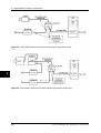
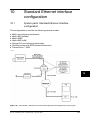
10 Standard Ethernet interface configuration ..................................................................................
10.1 System parts: Standard Ethernet interface configuration ....................................................
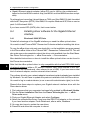
10.2 Software limitations ..............................................................................................................
10.3 PC recommendations ...........................................................................................................
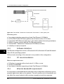
10.4 Ethernet bandwidth requirements ........................................................................................
10.5 Troubleshooting the standard Ethernet interface installation ..............................................
93
93
94
94
94
95
11 Disk management ...........................................................................................................................
11.1 About Ultra DMA and SATA disks ........................................................................................
11.2 Creating stripe sets and formatting NTFS disks in Windows ..............................................
11.2.1 Windows NT 4.0 stripe sets ..................................................................................
11.2.1.1
Partition the burst disks in Windows NT 4.0 .....................................
11.2.1.2
Format the burst disks in Windows NT 4.0 .......................................
11.2.2 Windows 2000/XP striped volumes ......................................................................
11.2.2.1
Creating and formatting striped volumes in Windows 2000/XP .......
97
97
97
97
98
98
98
98
Publ. No. T559009 Rev. a387 – ENGLISH (EN) – August 28, 2009
xi
11.2.2.2
Importing striped volumes in Windows 2000/XP .............................. 99
12 OLE tricks & tips ............................................................................................................................. 101
12.1 OLE in brief ........................................................................................................................... 101
12.1.1 Copying information to other applications ........................................................... 101
12.1.2 Linking into other applications ............................................................................. 101
12.1.3 Embedding into other applications ...................................................................... 101
12.1.4 Automation ............................................................................................................ 102
12.2 OLE caveats .......................................................................................................................... 102
12.2.1 Colors .................................................................................................................... 102
12.2.2 Incorrect aspect ratio ............................................................................................ 103
12.2.3 Multiple links do not update in Microsoft® Word ................................................. 103
12.2.4 Microsoft® Word consumes lots of disk space for live images ........................... 103
12.2.5 Microsoft® Excel does not accept our numerical values .................................... 103
12.2.6 Security warnings with Microsoft® Excel 2007 files ............................................ 104
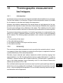
13 Thermographic measurement techniques ................................................................................... 105
13.1 Introduction .......................................................................................................................... 105
13.2 Emissivity .............................................................................................................................. 105
13.2.1 Finding the emissivity of a sample ....................................................................... 106
13.2.1.1
Step 1: Determining reflected apparent temperature ....................... 106
13.2.1.2
Step 2: Determining the emissivity ................................................... 108
13.3 Distance ................................................................................................................................ 109
13.4 Reflected temperature .......................................................................................................... 109
13.5 Atmospheric temperature, humidity and distance ............................................................... 109
13.6 External optics transmission and temperature .................................................................... 110
13.7 Infrared spectral filters .......................................................................................................... 110
13.8 Units of measure ................................................................................................................... 110
14 About FLIR Systems ....................................................................................................................... 113
14.1 More than just an infrared camera ....................................................................................... 114
14.2 Sharing our knowledge ........................................................................................................ 114
14.3 Supporting our customers ................................................................................................... 114
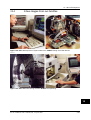
14.4 A few images from our facilities ........................................................................................... 115
15 History of infrared technology ...................................................................................................... 117
16 Theory of thermography ................................................................................................................ 121
16.1 Introduction ........................................................................................................................... 121
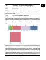
16.2 The electromagnetic spectrum ............................................................................................ 121
16.3 Blackbody radiation .............................................................................................................. 122
16.3.1 Planck’s law .......................................................................................................... 123
16.3.2 Wien’s displacement law ...................................................................................... 124
16.3.3 Stefan-Boltzmann's law ......................................................................................... 126
16.3.4 Non-blackbody emitters ....................................................................................... 127
16.4 Infrared semi-transparent materials ..................................................................................... 129
17 The measurement formula ............................................................................................................. 131
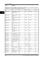
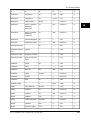
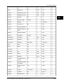
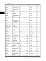
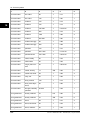
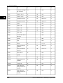
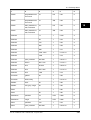
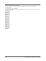
18 Emissivity tables ............................................................................................................................. 137
18.1 References ............................................................................................................................ 137
18.2 Important note about the emissivity tables .......................................................................... 137
18.3 Tables .................................................................................................................................... 138
xii
Publ. No. T559009 Rev. a387 – ENGLISH (EN) – August 28, 2009
1
Notice to user
Typographical
conventions
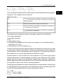
This manual uses the following typographical conventions:
■
■
■
■
User-to-user
forums
1
Semibold is used for menu names, menu commands and labels, and buttons in
dialog boxes.
Italic is used for important information.
Monospace is used for code samples.
UPPER CASE is used for names on keys and buttons.
Exchange ideas, problems, and infrared solutions with fellow thermographers around
the world in our user-to-user forums. To go to the forums, visit:
http://www.infraredtraining.com/community/boards/
Additional license
information
This software is sold under a single user license. This license permits the user to install
and use the software on any compatible computer provided the software is used on
only one computer at a time. One (1) back-up copy of the software may also be made
for archive purposes.
Publ. No. T559009 Rev. a387 – ENGLISH (EN) – August 28, 2009
1
1 – Notice to user
1
INTENTIONALLY LEFT BLANK
2
Publ. No. T559009 Rev. a387 – ENGLISH (EN) – August 28, 2009
2
Customer help
General
For customer help, visit:
2
http://flir.custhelp.com
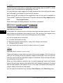
Submitting a
question
To submit a question to the customer help team, you must be a registered user. It
only takes a few minutes to register online. If you only want to search the knowledgebase for existing questions and answers, you do not need to be a registered user.
When you want to submit a question, make sure that you have the following information to hand:
■
■
■
■
■
■
Downloads
The camera model
The camera serial number
The communication protocol, or method, between the camera and your PC (for
example, HDMI, Ethernet, USB™, or FireWire™)
Operating system on your PC
Microsoft® Office version
Full name, publication number, and revision number of the manual
On the customer help site you can also download the following:
■
■
■
■
■
Firmware updates for your infrared camera
Program updates for your PC software
User documentation
Application stories
Technical publications
Publ. No. T559009 Rev. a387 – ENGLISH (EN) – August 28, 2009
3
2 – Customer help
2
INTENTIONALLY LEFT BLANK
4
Publ. No. T559009 Rev. a387 – ENGLISH (EN) – August 28, 2009
3
Welcome!
Thank you for choosing ThermaCAM™ Researcher Professional!
This is the operator's manual of ThermaCAM™ Researcher Professional. We are
convinced that this program will be a useful tool when you explore the fascinating
world of infrared imaging and measurements.
ThermaCAM™ Researcher Professional supports six hardware configurations:
■
■
■
■
■
■
Standard Ethernet
Gigabit Ethernet
FireWire
PC-Card
Parallel
IRFlashLink
The interfaces are used for several types of cameras. The manual, together with the
Camera Connections manual, covers all configurations and all cameras. Make sure
that the information you read is about the right camera with the right type of camera
interface.In the manual, you should be able to find detailed answers to these three
types of questions:
■
■
■
What kind of hardware and software is used? How is it to be installed?
What is the software and thermography like, in general?
How should I use ThermaCAM™ Researcher Professional, to get some particular
result?
Since this is more like a reference manual than a tutorial, there will be rather detailed
answers to those questions. It means that you probably only will study the manual in
parts from time to time.
If you need the manual, but cannot find it, you can rely on that the same information
is available as the help text of the program.
3.1
New features in ThermaCAM™ Researcher
Professional 2.9
ThermaCAM™ Researcher Professional 2.9 has a number of changes mainly regarding
the following:
■
■
■
Text comments in ThermaCAM™ SC640 were previously ignored. This behavior
has been corrected.
Connection to ThermoVision™ A320 and A320G is now provided.
Better handling of low battery/hibernate during recordings.
Publ. No. T559009 Rev. a387 – ENGLISH (EN) – August 28, 2009
5
3
3 – Welcome!
■
■
The subtraction preview did not always display the correct images.
Support for Windows Vista
3
6
Publ. No. T559009 Rev. a387 – ENGLISH (EN) – August 28, 2009
4
Installation
4.1
Installation instructions
The ThermaCAM™ Researcher Professional CD-ROM contains all software manufactured by FLIR Systems AB that you need in order to run ThermaCAM™ Researcher
Professional with:
■
■
■
■
■
■
a FireWire Interface
a PC-Card® Interface
an IC2-DIG16 frame grabber
an IRFlashLink board
a Gigabit Ethernet interface
a standard Ethernet interface
4
For the IRFlashLink board, you also need a CD-ROM from its manufacturer.
The installation procedures for these configurations differ, so please follow only the
instructions that are appropriate for your particular configuration.
The installations are two-step procedures. It is recommended that you install ThermaCAM™ Researcher Professional first, before the installing the camera interface device
drivers, but that order is only required for Windows 98.
4.1.1
Requirements
ThermaCAM™ Researcher Professional runs on Windows 2000, Windows XP (32-bit
edition), and Windows Vista (32-bit edition). ThermaCAM™ Researcher Professional
might also run on Windows 98/ME, Windows NT 4.0 (service pack 3 or higher), but
full functionality and performance cannot be expected.
The following exceptions exist:
■
■
■
■
The FireWire interface for image frame grabbing, as well as ThermoVision™ A320,
require Direct-X 8.1 (or higher). Since the FireWire technology is quite new to
Windows, we recommend that the most recent service packs and Windows updates
are installed on Windows 2000 and Windows XP. Updates from the computer
manufacturer web site may also be required.
There is no support for the FireWire interface on Windows NT 4.0, and Windows
98 (first edition)
The IRFlashLink Frame Grabber requires Windows 2000, XP or NT 4
Maximum speed image recording (burst recording) is only possible if the speed
of the hard disk I/O is sufficient. If you intend to use IDE Ultra DMA 100 disks, you
have to have at least Windows XP or service pack 2 of Windows 2000 to make them
work.
Publ. No. T559009 Rev. a387 – ENGLISH (EN) – August 28, 2009
7
4 – Installation
■
■
■
4
■
If you install a PC-Card® interface on Windows NT 4.0, you will also need the
CardWare software (version 6.00.007 or higher) from Unicore Software Inc.
(www.unicore.com)
The Gigabit Ethernet interface requires a network interface compatible with the Intel
82540 network chip for optimum performance (Intel 82541 and 82546 are also acceptable).
The PC-Card®, IC2-DIG16 and IRFlashLink interfaces cannot be combined with
usage of the ThermoVision™ SC4000/SC6000/A320/A320G cameras and cannot
be installed on Windows Vista.
For the Gigabit Ethernet interface, Windows 2000, XP, or Vista is required
4.1.2
Installing ThermaCAM™ Researcher Professional
We recommend that you first close all applications running on your computer (except
for antivirus and firewall software).
If you have Windows NT 4.0, 2000 or XP, please log in as the Administrator during
the installations.
4.1.2.1
Installation of the application software
ThermaCAM™ Researcher Professional is installed by an installation utility program.
It will guide you through the installation steps, and do most of the work. Just insert
the CD-ROM and choose to start the installation of ThermaCAM™ Researcher Professional from the installation window that appears.
During the installation, you will be asked to type in the license number. Your license
number is unique, and can be found on the first page of the manual.
The directory structure of ThermaCAM™ Researcher Professional is pre-set. The only
adaptation you can make to it is to change the name of the directory in which the
program is installed.
You will be asked about which type of cameras you intend to use, in order to avoid
installation of too many different drivers.
When the installation finishes, you may have to restart your computer.
After this installation, you will be able to start ThermaCAM™ Researcher Professional
from the Programs entry of the Start button menu.
4.1.2.2
Installation of the Direct-X software
With the FireWire interface, and with the ThermoVision™ A320 camera, Direct-X 8.1
(or higher) is required. In that case, the ThermaCAM™ Researcher Professional installation looks for Direct-X, checks its version and tells you to install it if needed. The
installation window offers you the possibility to install Direct-X 8.1 from the CD-ROM.
8
Publ. No. T559009 Rev. a387 – ENGLISH (EN) – August 28, 2009
4 – Installation
4.1.2.3
Installation of the camera interface driver software
When the application installation is finished, you will be reminded about the camera
interface driver software installation. You will not be able to connect to the camera,
only to work with images stored on disk, until you have installed this software.
The plug-and-play FLIR Systems camera interface drivers can be found on the ThermaCAM™ Researcher Professional CD-ROM, as well as in the directory C:\Program
Files\FLIR Systems\Device Drivers, to which the ThermaCAM™ Researcher Professional installation program copies them (except for the device drivers for the eBus
Driver Suite). When you install your device drivers, you can find all necessary FLIR
Systems files there.
4.1.2.4
Installation of the eBus Driver Suite
NOTE: Before you try this, make sure that your computer is fully updated by Windows® Update.
To take full advantage of an Intel 82540 Gigabit Ethernet Network Adapter you need
to install and activate the eBus Driver Suite, available on the ThermaCAM™ Researcher
Professional CD-ROM in the eBus folder. The installation just copies the drivers to
your hard disk drive. To activate a particular driver, you have to run a program from
the Start menu. Select Pleora Technologies, Inc., eBus Driver Suite and Driver Installation Tool. Pick the right Ethernet adapter and select Configure. Select the optimum eBus driver and click Finish.
You may also have to click Update to update the drivers as well.
SEE ALSO: For information about how to install the device drivers for the FireWire interface, as well as
other device drivers, see:
■
■
8 – FireWire™ configuration on page 81
Camera connections (Publ. No. T559010)
4.2
Where do the installed files go?
On all Windows systems, the installation program builds a new directory tree, normally
at C:\Program Files\ThermaCAM™ Researcher Professional\, containing the following
files:
ThermaCAM™ Researcher Professional\
Executable files, help file, OLE type library.
…\Examples
Sample Microsoft® Excel files with their session files
…\Images
Sample image files
…\Palettes
Palette files (scale color definitions)
...\Binaries
dll:s and controls related to the Indigo camera
Publ. No. T559009 Rev. a387 – ENGLISH (EN) – August 28, 2009
9
4
4 – Installation
The installation also adds some executable files into the main Windows directories,
and a number of device drivers to the C:\Program files\FLIR Systems\Device drivers
directory.
On Windows 2000, Windows XP, and Windows Vista, which are multi user systems,
only administrator users may create and update files in the common Program Files
directory. Ordinary users are not permitted to do that. Ordinary users have a place
of their own where they can keep the data files of their programs. It is called My
Documents.
4
On Windows 2000, Windows XP, and Windows Vista, the \Examples, \Images and
\Palettes files are copied to a ThermaCAM™ Researcher Professional subdirectory
of the My Documents directory of each user when he, or she, starts to use the software.
Then each user easily can modify them separately.
NOTE: These My Document files are not removed when you remove the program.
10
Publ. No. T559009 Rev. a387 – ENGLISH (EN) – August 28, 2009
5
About the program
5.1
Basic principles for ThermaCAM™ Researcher
Professional
The main purpose of this program is to deal with live IR images arriving through a
camera interface. It can also receive IR images from other media, such as SD Memory
Cards from ThermaCAM™ cameras.
The program can make studies on high/medium/slow speed thermal events depending
on the hardware configuration. It can show IR images, record them on disk and
analyse them afterwards during their replay. It can provide measurement result values
directly from the live stream of images too, but only for the images you decide not to
record.
The measurements are made with the following analysis tools: isotherm, spotmeter,
area and line. The results produced by these tools can be displayed within the IR
image, in the profile window, in the histogram window, in the result table window, or
in the plot window. Formulas can be applied to the results.
The program uses a set of predefined screen layouts, one for each type of work that
you could have in mind.
You can also extract information from ThermaCAM™ Researcher Professional by using
OLE (which is an automatic way of transferring information between programs running
under Windows) to bring the information into for example Microsoft® Excel or Microsoft® Word. The IR image can be transferred in the same way. The clipboard
functions Copy and Paste are used for this purpose.
Several copies of ThermaCAM™ Researcher Professional can run at the same time,
but only one at a time can be connected to the same camera.
5.2
Working with ThermaCAM™ Researcher Professional
A typical user of ThermaCAM™ Researcher Professional would probably install it both
on a laptop computer, which easily can be brought along to the site where the data
is to be collected, and on a stationary computer connected to a network with printers
and disks on it.
At the site, the user would set up the camera, connect it to the computer and start
recording.
Some users will record images, lots of images, and go back home in order to study
them. Others will immediately make measurements and simply record a few values
on paper or in a spreadsheet and forget about the images on which they are based.
Publ. No. T559009 Rev. a387 – ENGLISH (EN) – August 28, 2009
11
5
5 – About the program
Some users are satisfied with the temperature measurements as such, others want
mathematical functions of temperature or to correlate the measurements to something
else, like pressure or vibration or the incidence of some event.
Being careful when setting up the camera will normally improve the measurement
results. This could mean measuring the object parameters carefully, avoiding creating
images containing reflections from strong heat (or cold) sources in the neighbourhood,
using a spectral IR-filter which is appropriate for the application and so on.
5
Before studying the recorded images, one has to pick out and examine the really interesting ones. Then one normally finds that something has to be done to them before
the actual analysis begins. The emissivity factor might be wrong, or the temperature
scale limits or the analysis tool is missing or whatever. The images recorded by
ThermaCAM™ Researcher Professional do not contain any analysis; it has to be
added on.
In this preparatory step, the user will scan through all the images, noting the interesting
ones, grouping them and preparing them for analysis. This involves either applying
a correction to each individual image, actually changing the file, or using a standard
correction replacing some parameter of the images but not changing the images
themselves.
The standard correction is, in this program, often indicated by the word lock. It is
possible to lock the temperature scale, lock the object parameters the analysis functions and lock the zoom factor. This means for instance that you can apply your
favourite temperature scale to an image by locking the scale and setting it to your
favourite values. The current image, and the ones that follow, will be presented with
your favourite scale despite having another scale stored inside them. When you unlock
the scale, the original scale of the image will reappear.
The actual analysis involves playing through the images once more, taking values
from the analysis tools of the images and comparing them to what was expected.
The analysis might be preceded by a conversion of some kind, such as image subtraction.
The results of the study might become an important part of a research report, a graph
or a set of images supporting some vital conclusion.
5.3
List of current image files
When you store images with ThermaCAM™ Researcher Professional you can either
store them one by one, giving each image a characteristic file name, or store them
as a sequence thus indicating that they have something in common.
12
Publ. No. T559009 Rev. a387 – ENGLISH (EN) – August 28, 2009
5 – About the program
Such a sequence of IR images is recorded in an image directory either as separate
files or in a single file. This is a decision you take when you set the recording parameters.
When the recording is finished, the sequence recording function assumes that you
would like to replay and analyse the new images. It creates a list of the image files
concerned and keeps it until the next recording.
This list, a group of names of image files in the same directory, is what still keeps the
sequence together. You may change the list at will, adding or removing file names,
but then the sequence concept is lost.
You can actually group any images you like into a fake sequence. The only restriction
is that they have to be stored in the same directory on the disk. You do not have to
include all the images of the directory.
Single file image recordings are normally quite large. ThermaCAM™ Researcher
Professional has functions that will let you edit these files. Then you are supposed to
first open all images and then mark the images to be removed or copied as a selection.
5.4
Image directory
All the images of the same recording are placed in the same directory on disk. We
call it the image directory. The full path name of the image directory is displayed in
the program title bar. You should set it when you determine the conditions for image
recording (or when you create a new image list out of pre-recorded images).
5.5
Session files
You often need to be able to recreate particular situations (such as an experiment)
during your work. ThermaCAM™ Researcher Professional uses session files for this
purpose. It stores for example the names of the currently open images in its session
files. They do however not contain the images themselves. You will notice this, if you
save your session while looking at a frozen live image. When the session is recreated,
the former live image is gone.
The full path name of the image directory is also stored in the session file.
If you move the images (or try to reach them from another computer in which the
image directory has another path), you will have to correct this path in order to be
able to see the images again.
Normally, every recording of images would be ended with the creation of a session
file. It would usually be placed in the same directory as the images, but that is not a
requirement. Later, when you start analysing the images, you pick up the session file,
Publ. No. T559009 Rev. a387 – ENGLISH (EN) – August 28, 2009
13
5
5 – About the program
add analysis tools or other settings to it and save it to disk again. The session files
do not contain any images or analysis results, only file names and information about
the program settings.
You may select a session file to become the default session. This means that every
time you start ThermaCAM™ Researcher Professional or order a brand new session,
the default session settings and images will be fetched. The Set Default Session
command is in the File menu.
Should you wish to avoid reading the default session, press SHIFT while ThermaCAM™
Researcher Professional starts.
5
You deselect the default session by opening the default settings dialog box and
clicking the Cancel button.
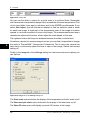
5.6
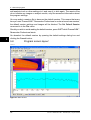
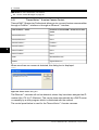
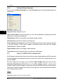
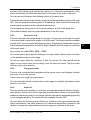
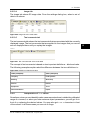
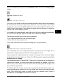
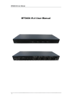
Program screen layout
10426603;a3
Figure 5.1 Main window
14
Publ. No. T559009 Rev. a387 – ENGLISH (EN) – August 28, 2009
5 – About the program
There are several layout options available. These are controlled by tabs in the bottom
part of the ThermaCAM™ Researcher Professional window. You can see combinations
of the IR image, the profile, the histogram, the plot and the result table windows. All
tabs have an IR image with a temperature scale in the top left corner.
You cannot reposition the windows within the tabs, but you can catch and move the
splitter bars that separate the windows, thus increasing or decreasing the relative
size of each of the windows.
You can copy the whole program window to the clipboard by pressing the ALT +
PRINTSCRN key buttons. You can also save the current tab as a bitmap by the
command Save Tab As in the File menu
The program can only show one image at a time. On the image, the analysis tools
are displayed. The results of the analysis tools can be displayed in the histogram,
profile, plot or result table window.
The main layout of the program is pretty much like any other Windows program. On
the top line of the program window, there is a title containing a session name, the
image directory and the three buttons, minimise, maximise and close, from left to
right. The same functions are available on the right mouse button menu of the top
line.
Below the top line, there is a set of drop-down menus by which you can select functions related to session/image filing (File), the clipboard (Edit), the screen layout
(View), the camera (Camera), the display and analysis of the image (Image) and the
recording/playback of images (Recording).
There is also a large number of toolbar buttons. There are toolbar buttons for almost
every function of the program. Every toolbar button has a short yellow description
that will pop up if you hold the mouse cursor still for a while on top of it.
The toolbars are normally docked to the borders of the program window, but can be
undocked and placed anywhere on the screen. Just double-click on them.
There is also a floating camera control panel that can not be docked to the program
window. Use it to change the camera settings and affect how the live image is generated.
At the bottom of the program window, on the status line, a more detailed description
of the menu items and tool bar buttons will be shown while you sweep through menus
and over the toolbar buttons by the mouse cursor. Towards the right of this status
line, there are indicators of the Interface status and the Camera status as well as
keyboard indicators for Caps Lock and Num Lock. You can click on the Interface
and Camera indicators and get further information about the interface and the camera.
Publ. No. T559009 Rev. a387 – ENGLISH (EN) – August 28, 2009
15
5
5 – About the program
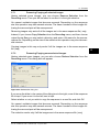
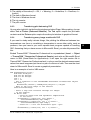
5.6.1
Standard toolbar
10417703;a2
Figure 5.2 Standard toolbar
From left to right:
■
■
■
■
Create a new session
Open an existing session
Open/add images to the current session
Save the current session using the current name
10417803;a2
5
Figure 5.3 Standard toolbar, continued
From left to right:
■
■
■
■
Copy the session file and the current image to the clipboard
Copy values, such as analysis results, as text to the clipboard
Paste a copied session into ThermaCAM™ Researcher Professional. The name of
the session is not pasted.
Print the current image
10417903;a2
Figure 5.4 Standard toolbar, continued
From left to right:
■
■
■
■
■
■
■
■
■
Select disk images as the image source
Select the live camera as the image source.
Move the camera focus towards infinity
Autofocus the camera
Move the camera focus towards the lens
Switch on the function automatic adjustment of the image scale
Freeze the live stream of images from the camera
Bring up the image settings dialog box
Bring up the palette selection dialog box
10418003;a2
Figure 5.5 Standard toolbar, continued
■
Bring help from the manual
16
Publ. No. T559009 Rev. a387 – ENGLISH (EN) – August 28, 2009
5 – About the program
5.6.2
Play images toolbar
10418103;a2
Figure 5.6 Play images toolbar
Top row:
■
■
■
■
Show second row: ON/OFF
Name of the current image. You may type a name or number in this field.
7 VCR style playback buttons. Stop in the middle.
A control by which the replay rate is controlled
■
■
■
■
■
■
■
■
5
*1 means full speed from disk
*2 means twice full disk speed (i.e. every other image is not shown)
÷2 means half full speed
Auto rewind button
Lock temperature scale button
Lock object parameters button
Lock analysis tools button
Lock zoom factor button
The Lock buttons will, when pressed, let you keep the same temperature scale / object
parameters / analysis tools / zoom factor for all images being replayed, regardless
of what is stored inside the images. When you depress these buttons, the information
of the images will be used instead.
Second row:
■
■
■
■
■
■
Current image time/frame/trig count
First image time/frame/trig count
Slider. Move fast within your image sequence. The first image is to the left.
Last image time/frame/trig count. The time/frame/trig count field depends on the
Presentation selection in Replay Settings in the Recording menu. It is either absolute image time, relative time to first frame, frame number or trig count.
Set selection start
Set selection end
Start is always to the left of End. The slider will highlight the selected area within the
sequence with a blue color.
Publ. No. T559009 Rev. a387 – ENGLISH (EN) – August 28, 2009
17
5 – About the program
5.6.3
Recording toolbar
10418203;a2
Figure 5.7 Recording toolbar
Left to right:
5
■
■
■
■
■
■
■
■
■
■
Name of the next image to be recorded
Start button
Start condition field
Record one image button
Recording condition field
Pause button
Stop button
Stop recording condition field
Bring up the recording conditions dialog box
Replay the recorded sequence in a separate copy of ThermaCAM™ Researcher
Professional
5.6.4
Image dir toolbar
10418303;a1
Figure 5.8 Image dir toolbar
■
■
The image directory. You may edit this field to change it.
Browse existing directories
5.6.5
Analysis toolbar
The following analysis tools exist (left to right):
10418403;a1
Figure 5.9 Analysis toolbar
From left to right:
■
■
■
■
■
■
■
■
Spot meter
Flying spot meter. Uses the mouse cursor.
Line, with cursor
Box area
Circle area
Polygon area
Isotherm (above, below, interval)
Formulas
18
Publ. No. T559009 Rev. a387 – ENGLISH (EN) – August 28, 2009
5 – About the program
■
Removal tool
5.6.6
Scaling toolbar
10418503;a2
Figure 5.10 Scaling toolbar
From left to right:
■
■
■
■
■
■
Scale max temperature field. Editable.
Scale min temperature field. Editable.
Current measurement unit indicator
Slider for the scale max and min temperature. Drag with mouse. Min is to the left.
Automatic adjustment of the scale to the image: ON/OFF
Lock span: ON/OFF. Changes apply only to the level.
The highlighted region in the sliders indicates the span of temperatures in the image.
By selecting Auto Adjust, you will place the slider markers close to the ends of the
highlighted area, but still inside it. A small part of the span is thus wasted.
5.7
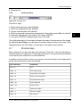
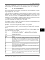
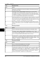
Shortcut keys
Menu selections can be made from the keyboard. Press Alt + the key indicated on
the menu line by an underscore. This brings up the menu. Then press the key indicated
in the menu by an underscore to select that item.
In addition to the tool bars, there are a number of shortcut keys on the keyboard by
which important functions can be reached:
Key combination
Explanation
ALT + F4
Exit
CTRL + A
Auto adjust image
CTRL + C
Copy session and image
CTRL + D
Play recorded sequence
CTRL + F
Freeze/Unfreeze image
CTRL + F2
Step backwards
CTRL + F4
Step forwards
CTRL + I
Open disk images
CTRL + L
Show live images
CTRL + N
New session
Publ. No. T559009 Rev. a387 – ENGLISH (EN) – August 28, 2009
19
5
5 – About the program
5
Key combination
Explanation
CTRL + O
Open session
CTRL + P
Print
CTRL + PAGE UP/DOWN
Changes max scale temperature
CTRL + R
Autorewind mode on/off
CTRL + S
Save session
CTRL + SHIFT + F2
Set selection start (within sequence)
CTRL + SHIFT + F4
Set selection end (within sequence)
CTRL + SHIFT + TAB
Previous main tab
CTRL + T
Show the camera control
CTRL + TAB
Next main tab
CTRL + V
Paste session
END
Last disk image
F2
Play backwards
F3
Stop playing
F4
Play forwards
F5
Image recording keyboard trig
F8
Freeze/Unfreeze image
F9
Camera autofocus
F11, F12
Camera focus
HOME
First disk image
PAGE UP/DOWN
Changes min scale temperature
SHIFT + F2
Fast backwards
SHIFT + F3
Stop
SHIFT + F4
Fast forwards
NOTE: Some shortcuts do not work in OLE embedded mode.
20
Publ. No. T559009 Rev. a387 – ENGLISH (EN) – August 28, 2009
6
Tutorials
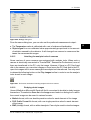
6.1
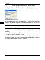
How to begin using a camera
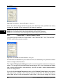
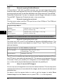
We recommend that you connect the cables and start the camera before starting the
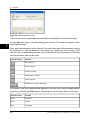
ThermaCAM™ Researcher Professional program. The first time you run ThermaCAM™
Researcher Professional, you will have to indicate which type of camera you have
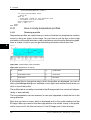
got and how it is connected physically. This dialog box automatically shows up:
10418603;a5
6
Figure 6.1 Select camera dialog box
You do have to bring up this dialog box yourself (from the Camera menu), if you want
to change the selected camera type or connection.
Publ. No. T559009 Rev. a387 – ENGLISH (EN) – August 28, 2009
21
6 – Tutorials
6.2
How to connect and control the camera
SEE ALSO: For information about begin using the camera with older types of connections (PC-Card,
parallel interface, IRFlashLink etc), see the following documents on the CD:
■
■
■
Installation Hints (Publ. No. T559004)
System configurations (Publ. No. 1 557 783)
Camera connections (Publ. No. T559010)
In order to be able to show a live image, ThermaCAM™ Researcher Professional has
to establish a software connection to the camera. The status information of the
Camera Control panel will reveal if the program is trying to connect to the camera or
not. If it says Disconnected, you will have to order a new connection by selecting
Connect from the Camera menu.
On the same menu, there is a Normalized connection command which sets the
camera in a state suitable for almost any computer during the connection process.
6
If ThermaCAM™ Researcher Professional is showing a disk image, you will have to
select Show Camera Image from the Camera menu or press CTRL + L or click this
toolbar button to make the program consider connecting to the camera and displaying
its image.
10418703;a2
Figure 6.2 Show camera image toolbar button
The purpose of doing these soft connections/disconnections is that it enables you to
run two or more copies of ThermaCAM™ Researcher Professional. You can disconnect
the camera from one copy and connect it to another instead.
If you have two (or more) FireWire cameras, you can connect each camera to a separate copy of ThermaCAM™ Researcher Professional, perhaps with a slight loss of
performance.
After the connection is established, it may still take some time before the logo image
disappears. The camera may have to run for a while, before its detector is cool enough
to produce a live image.
SEE ALSO: If you get into connection difficulties here, see section:
6.2.4 – About connection difficulties on page 30
NOTE: Do not remove the FireWire cable or switch off the camera while ThermaCAM™ Researcher
Professional is running unless you have selected Disconnect from the Camera menu first.
■
The Camera Information dialog box and the Camera Control panel are the two main
ways by which you communicate with the camera.
22
Publ. No. T559009 Rev. a387 – ENGLISH (EN) – August 28, 2009
6 – Tutorials
Take a quick look at the Camera Information dialog box, which can be reached from
the Camera menu or by clicking on the camera symbol to the right on the status line
below the image. It will probably show the name of the camera and that it is working.
Otherwise the reason of failure is displayed here (or in the Device Status panel displayed if you click on the interface symbol to the lower right of the program window).
Let’s take a quick look at the Camera Control panel. We will study it in more detail
in the next sub-chapters.
Let’s examine the Measurement Range list on the second tab. Select a range, which
covers the expected measurement temperatures. The range limits are blackbody
temperatures, so if your measurement target has a shiny surface with a low emissivity,
you will be able to make measurements above the range limits.
An image, which is probably blurry, is shown on the screen. Otherwise, click the
candle toolbar button to get a better scale in the PC. Some cameras have their own
ways of adjusting the image and improving its quality. See the appropriate camera
control description below.
10418803;a2
Figure 6.3 Candle toolbar button
Aim the camera onto the target. Focus the camera, either by using the focus buttons
on the Camera Control panel or the three buttons below (found on the standard
toolbar). You also have the option to use the F9/F11/F12 keys.
10418903;a2
Figure 6.4 Focus toolbar buttons
Click the arrow target button to autofocus the camera.
Hold down the other buttons in order to run the focus motor of the camera towards
infinity or towards the lens. Release the button when the focus is OK, or rather
slightly before. There is a small delay before the focus motor stops.
If you are satisfied with your image, you can freeze it by clicking this button on the
standard toolbar or pressing CTRL + F or F8:
10419003;a2
Figure 6.5 Freeze toolbar button
If it is an interesting image, you had better save it on disk right now. If you leave the
program without first recording the image, the image is lost.
Publ. No. T559009 Rev. a387 – ENGLISH (EN) – August 28, 2009
23
6
6 – Tutorials
SEE ALSO: For more information, see section:
■
6.5 – How to record IR images on page 34
6.2.1
ThermoVision™ A-series Camera Control
ThermaCAM™ Researcher Professional allows you to connect A-series cameras either
through a FireWire™ interface or through an Ethernet™ interface.
6
ThermoVision™ model
Interface to ThermaCAM™ Researcher Professional
A20 M/V Ethernet™
None
A40 M/V Ethernet™
None
A20 M FireWire™
FireWire™
A40 M FireWire™
FireWire™
A20 V FireWire™
None
A40 V FireWire™
None
A320
Standard Ethernet™
A320G
Gigabit Ethernet™
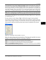
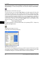
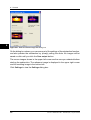
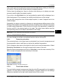
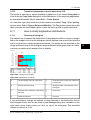
When more than one camera is detected, this dialog box is displayed.
10770203;a1
Figure 6.6 Select device dialog box
The Ethernet™ cameras will not be detected, unless they have been assigned an IPnumber (like 172.16.17.56 above). This can be done automatically by a DHCP server
or manually by a utility program which is distributed with the camera.
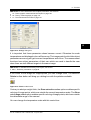
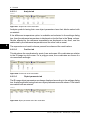
The control panel below is used for the ThermoVision™ A-series cameras.
24
Publ. No. T559009 Rev. a387 – ENGLISH (EN) – August 28, 2009
6 – Tutorials
10431203;a1
Figure 6.7 ThermoVision™ A-series FireWire™ dialog box
If some button is disabled on your camera control, it is because your particular camera
does not support that function.
The selected Measurement Range should cover the expected measurement temperatures. The range limits are blackbody temperatures, so if your measurement target
has a shiny surface with a low emissivity, you will be able to make measurements
above the range limits.
If you click the Int. Image Correction button on the Camera Control panel, the camera
will respond by making a rather heavy clicking sound when the internal shutter is
pulled and adjust its own temperature scale once to the current image. It is highly
recommended to use the Int. Image Correction function now and then, since it improves the image quality. Select the Auto shutter option if you want an automatic internal image correction. This automated process can be disabled as it may affect the
recording of images. When you switch it off, a warning will appear on the status field
of the control. This warning will become red if you leave it switched off for a long time.
NOTE: There is a related function in the Image menu, on the standard toolbar and on the scaling toolbar.
That function is called Auto Adjust. It will continuously adjust the scale to the image locally, within the PC.
If noise reduction is set to On, it will blur the image of moving objects.
If the camera is connected to the PC using the ThermaCAM™ Connect 2.0 software
and ThermaCAM™ Researcher at the same time, the live image may seem frozen.
The Downsample checkbox is only available for A20 cameras. This option affects
how much disk space each image will occupy when stored on the hard disk. If enabled,
disk space for each image will be significantly reduced. However, a performance
penalty (in terms of apparent image quality, but not in measurement) is introduced
when storing and reading image files.
Publ. No. T559009 Rev. a387 – ENGLISH (EN) – August 28, 2009
25
6
6 – Tutorials
10430703;a2
Figure 6.8 ThermoVision™ A-series FireWire™ dialog box
Select the desired frame rate from the list box. The frame rate specifies how many
images per second will be captured of the target in question.
6
NOTE: For cameras with a fixed frame rate, this selection will be unavailable.
NOTE: For some cameras, frame rates higher than 25/30 Hz may not be supported.
NOTE: For some computers, frame rates higher than 25/30 Hz may not work properly.
6.2.2
ThermaCAM™ S-series Camera Control
This control panel is used for ThermaCAM™ S60, ThermaCAM™ S40, ThermaCAM™
SC640, and similar camera models.
10419103;a1
Figure 6.9 ThermaCAM™ S-series FireWire™ dialog box
If some button is disabled on your camera control, it is because your particular camera
does not support that function.
The selected Measurement Range should cover the expected measurement temperatures. The range limits are blackbody temperatures, so if your measurement target
has a shiny surface with a low emissivity, you will be able to make measurements
above the range limits.
If you click the Int. Image Correction button on the Camera Control panel, the camera
will respond by making a rather heavy clicking sound when the internal shutter is
pulled and adjust its own temperature scale once to the current image. It is highly
26
Publ. No. T559009 Rev. a387 – ENGLISH (EN) – August 28, 2009
6 – Tutorials
recommended to use the Int. Image Correction function now and then, since it improves the image quality. Select the Auto shutter option if you want an automatic internal image correction. This automated process can be disabled as it may affect the
recording of images. When you switch it off, a warning will appear on the status field
of the control. This warning will become red if you leave it switched off for a long time.
NOTE: There is a related function in the Image menu, on the standard toolbar and on the scaling toolbar.
That function is called Auto Adjust. It will continuously adjust the scale to the image locally, within the PC.
At the bottom of the Cam tab, there are three focus buttons: Near focus (–), auto focus
(=) and far focus (+).
If noise reduction is set to Low or High, it will blur the image of moving objects.
The camera control will block the camera power down function to ensure proper operation during image recording. To prevent the camera from shutting down when
disconnected, make sure that the power down timeout is disabled in the camera.
10566703;a1
Figure 6.10 ThermaCAM™ S-series FireWire™ dialog box
Select the desired frame rate from the list box. The frame rate specifies how many
images per second will be captured of the target in question.
NOTE: For cameras with a fixed frame rate, this selection will be unavailable.
NOTE: For some cameras, frame rates higher than 25/30 Hz may not be supported.
NOTE: For some computers, frame rates higher than 7 Hz may not work properly.
NOTE: Use the Normalized connection command on the ThermaCAM™ Researcher Professional Camera
menu if connection fails due to a too high frame rate.
Publ. No. T559009 Rev. a387 – ENGLISH (EN) – August 28, 2009
27
6
6 – Tutorials
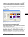
6.2.3
SC4000/SC6000 Camera Control
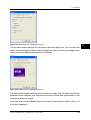
This control panel is used for ThermoVision™ SC4000/SC6000 cameras. It has a Cal
tab, a NUC tab, a Dev tab, and optionally a HSDR tab for calibration, non-uniformity
correction, device handling, and high speed data recording.
10755103;a1
6
Figure 6.11 Cumulus iPort – camera control tabs
If a button is disabled on your camera control, it is because your particular camera
does not support that function.
The Lens-Filter list contains the calibrated lenses and filters of your camera. The
Temperature Range list shows the calibrated ranges for the chosen lens and filter
in the first list. When you have selected your lens, filter and range, please press the
Apply button.
The calibration file of the camera is normally downloaded to your PC when you connect
to the camera for the first time. If you need to refresh this information, mark the
Download check box, disconnect and connect again.
The Name list on the NUC tab shows the NUC tables currently stored in the camera.
All tables are shown, not only those associated with a calibration. The tables contain
non-uniformity correction data, integration time, frame size and other settings. If you
select a NUC name from this list, you will switch to that table but get a non-calibrated
IR-image. To get a calibrated image, you have to use the controls on the Cal tab.
The Int.time field shows the current integration time in milliseconds.
To improve the image quality, you can apply an Internal or External Flatness correction. By allowing the camera to look at an internal or external thermally flat surface,
with a temperature well within the current temperature range limits, you can even out
many image distortions. Just press the Internal or External Flatness correction
buttons. You will not invalidate the current calibration if you do this, but the name of
28
Publ. No. T559009 Rev. a387 – ENGLISH (EN) – August 28, 2009
6 – Tutorials
the current NUC table is lost. The quality improvement can be considerable, especially
if external correction is used and the camera recently was switched on. The external
correction is better, because it also includes the lens non-uniformities.
The Frame Size list on the Dev tab shows a number of alternative image sizes for
calibrated cameras. If you reduce the frame size you can increase frame rate without
overloading the camera. Fill in a new value in the Frame Rate edit box and press
Change Rate to do this. The current maximum recommended frame rate is shown
above the button. Even if the camera doesn't get overloaded, your computer can still
have difficulties with high frame rates.
If you should happen to increase the frame size without remembering to reduce the
frame rate, ThermaCAM™ Researcher Professional will reduce it to 5 Hz for you.
If the camera somehow was set to conditions overloading the computer, use the
Normalised Connection alternative on the Camera menu to reset them when you
connect the camera.
The Camera Info button brings up a dialog window with information from the calibration of the camera.
The Device Status button shows information regarding the connection to the camera.
The HSDR tab will only show up if a ThermaCAM™ Researcher HSDR module is installed on the computer. The High Speed Data Recorder is a unit which captures a
very high speed raw pixel data stream from the camera and stores it directly on disk.
The recording can afterwards be converted into an image format suitable for ThermaCAM™ Researcher. The camera calibration will then be preserved.
You must pair the camera to the HSDR before you can begin using the HSDR Controller software to make HSDR recording.
It is not a very good idea to change the Frame Size setting in ThermaCAM™ Researcher Professional when you have precious data stored in the HSDR, since the
change will wipe out all stored data. When a HSDR recording is in progress, the frame
size list box will become disabled.
Publ. No. T559009 Rev. a387 – ENGLISH (EN) – August 28, 2009
29
6
6 – Tutorials
6.2.4
About connection difficulties
At times, you may run into difficulties establishing a connection with the camera. Here
are some suggestions on what you can do:
Problem
Possible cause & solution
The program is having problems with the camera.
It only works now and then.
Verify that the FireWire cable is properly connected
to the computer and the camera.
Always exit the program or select Disconnect from
the camera menu before you disconnect or switch
off the camera.
The program refuses to establish a contact with
the camera. The status information keeps saying
Disconnected while the camera is running.
The camera may be connected to another copy
of ThermaCAM™ Researcher Professional. Switch
over to that one and disconnect the connection.
Now the new ThermaCAM™ Researcher Professional can connect to the camera.
6
SEE ALSO: For information about begin using the camera with older types of connections (PC-Card,
parallel interface, IRFlashLink etc), see the following documents on the CD:
■
■
■
Installation Hints (Publ. No. T559004)
System configurations (Publ. No. 1 557 783)
Camera connections (Publ. No. T559010)
6.3
How to display an IR image
6.3.1
Obtaining a good IR image
In order to get a good image from the camera, you should establish a connection,
select an appropriate measurement range, auto adjust it, and focus it as described
in the previous chapters.
No matter if you have a live image, a frozen image or a disk image, you should now
consider the object parameters (emissivity, reflected temperature, atmospheric temperature, relative humidity of the air, the distance and the external optics transmission
and temperature). They describe the physical properties of the body of interest and
its environment and the atmosphere between the object and the camera. You can
reach them via Settings in the Image menu or this button:
10419903;a1
Figure 6.12 Image settings toolbar button
30
Publ. No. T559009 Rev. a387 – ENGLISH (EN) – August 28, 2009
6 – Tutorials
SEE ALSO: For more information about object parameters, see sections:
■
■
■
13 – Thermographic measurement techniques on page 105
16 – Theory of thermography on page 121
17 – The measurement formula on page 131
10426803;a2
6
Figure 6.13 Settings dialog box
It is important that these parameter values become correct. Otherwise the scale
temperatures and displayed colors will be wrong. The image parts for which the object
parameters are wrong will get incorrect temperatures and colors. The measurement
functions have object parameters of their own which are used to handle the case
when there are two different targets in the same image.
SEE ALSO: To calculate the emissivity of an object, see section:
■
6.8.9 – Emissivity calculation on page 59
If the colors of the image are inappropriate, you can change them. The selection
Palette toolbar button will bring up a dialog box with the palettes available.
10420103;a1
Figure 6.14 Palette toolbar button
Contrary to what you might think, the Show saturation colors option enables specific
coloring of image points, which are outside the current temperature scale. The Show
out of range colors option enables specific coloring of image points, which are outside
the detectable range of the camera.
You can change the temperature scale with this control bar:
Publ. No. T559009 Rev. a387 – ENGLISH (EN) – August 28, 2009
31
6 – Tutorials
10420203;a2
Figure 6.15 Control bar
You can use the slider to search for a good scale or to set fixed limits. Remember
that the maximum temperature always has to exceed the minimum temperature. Click
on the input fields if you want to edit them and hit the ENTER key afterwards. If you
select Auto Adjust, you will find that an attempt to find the optimum scale is made
for each new image. A small part of the temperature span of the image is however
wasted, to minimise the effect of noise in the image. The measurement areas have a
related auto adjustment function, which adjust the scale based on the area.
The rightmost button will keep the distance between the slider controls fixed.
6
Sometimes, when a live camera image is shown, you can find it impossible to change
the scale in ThermaCAM™ Researcher Professional. This is when the camera has
been set to continuously adjust the level or span of the image. Switch that camera
setting off.
Finally, in the Image tab of the Settings dialog box, there are a few more options you
can explore:
10426903;a2
Figure 6.16 Image tab of the Settings dialog box
The Show scale option switches the display of the temperature and color scale on/off.
The Show analysis labels option will switch the display of the label texts on/off.
The Show 3D-view option will display a pseudo-3D version of the image.
32
Publ. No. T559009 Rev. a387 – ENGLISH (EN) – August 28, 2009
6 – Tutorials
The Update temperatures option has to do with the update of OLE links, profile, histogram and result table when analysis tools are moved around in the image.
The Smooth drawing option makes the image appear to be less noisy, without affecting
the measurement results. Isotherms can look less crisp.
The Get analysis option should not be used unless your images contain analysis
tools that vary from image to image, which normally isn’t the case.
The Zoom factor makes it possible to temporarily enlarge the centre of an image.
6.3.2
Transferring an IR image with OLE
If you want to display your image in a program not designed for IR images, you have
to use OLE to make it visible. Use the Copy session and image toolbar button or the
same command of the Edit menu.
10420503;a1
6
Figure 6.17 Copy session and image toolbar button
6.4
How to trigger ThermaCAM™ Researcher Professional
from outside
If your target is active only on certain occasions, you might well want to tell the program
when it should examine at the target. Two functions in ThermaCAM™ Researcher
Professional work under such conditions. The recording functions that collect images,
and the plotting functions that collect measurement results.
They can conditionally record or plot not only at certain times, but also on external
trig pulses. The parallel interface has a trig input connector, which is the default trig
source. In addition, a free COM port or a LPT port can be used as the external trig
source.
The external trig increments a trig counter which is stored with each image. The value
of this counter can be displayed in the Play Images toolbar bar and the result table.
For COM or LPT trigs, the counter only counts one trig pulse per image.
The source for the external trig is selected from the Recording Conditions dialog box
in the camera control panels.
6.4.1
External trig using the parallel interface or IRFlashLink
SEE ALSO: For more information, see the following documents on the CD:
■
Camera connections (Publ. No. T559010)
Publ. No. T559009 Rev. a387 – ENGLISH (EN) – August 28, 2009
33
6 – Tutorials
6.4.2
External trig using FireWire/Ethernet
In ThermoVision™ A20, A40, and A320 cameras, you can mark image frames at the
instant an alarm was triggered. By doing so certain trigger information is assigned to
the image and the frame can be then identified in the image stream by ThermaCAM™
Researcher Professional. You can, for example, use this trigger information to make
ThermaCAM™ Researcher Professional start or stop a recording.
6.4.3
External trig using the serial port
This trig source option uses the CTS input line on a free COM port. The COM port
has an RS232 electrical interface.
Trig input using COM port
6
DSUB-25
Pin 5: Trig Input.
Transition Low (<-3 V) to High (>+3 V) =trig.
Close pin 4 and 5 to trig.
DSUB-9
Pin 8: Trig Input.
Transition Low (<-3 V) to High (>+3 V) =trig.
Close pin 7 and 8 to trig.
SEE ALSO: For a more detailed description of the electrical interface, read the RS-232 specification.
6.4.4
External trig using the printer port
The printer port (LPT) option is only available on Windows 95/98/ME platforms. This
trig source option uses a control signal on a free LPT port. The LPT port has a TTL
electrical interface.
Trig input using LPT1 (or LPT2) DSUB 25 pin printer port.
Pin 10: Trig Input.
Open circuit = high. (+2.4 V to + 5 V)
Transition High -> low =trig.
Pin 22: Ground
Closing 10 - 22 = trig.
The LPT1 port is normally associated with the physical hexadecimal address 378 and
the LPT2 port is associated with address 278. The camera control assumes that this
is the case. Check your parallel port configuration in the Control Panel → System
icon, to find out the physical address associated with the parallel port.
6.5
How to record IR images
You can only record images that come from the camera interface. The currently active
measurement tools are not recorded with the images, but the current scale and object
parameters are.
You have to click the camera button in order to get live images (or select Show
Camera Image from the Camera menu or press CTRL + L on the keyboard).
34
Publ. No. T559009 Rev. a387 – ENGLISH (EN) – August 28, 2009
6 – Tutorials
10420603;a2
Figure 6.18 Camera toolbar button
6.5.1
Recording toolbar
When the camera becomes the image source, the following toolbar is displayed.
10420703;a2
Figure 6.19 Recording toolbar
It is primarily associated with recording sequences of image files, but can also be
used to record single image files. The leftmost field shows the name of the file that
will be stored next. The name consists of a base part (NEW) to which a sequence
number is added (0002) and extension is appended (.IMG or .SEQ). The base part
is a text string, which you can change in the Recording Conditions dialog box hidden
under the stopwatch button on the same toolbar. The sequence number is controlled
by ThermaCAM™ Researcher Professional and is increased by 1 for every image file
or image sequence file.
A field showing the current condition for starting the recording follows the toolbar
button with the start pistol.
A field showing the current condition for recording an image follows the toolbar button
with the disk. No matter what the field says, the diskette button will always record one
image, even if the start condition is not fulfilled.
The next button will temporarily stop the recording: Pause.
A field showing the current condition for stopping the recording follows the toolbar
button with the chequered flag. No matter what the field says, the flag button will always
stop the recording.
The second last button will bring up the Recording Conditions dialog box.
The very last button will start the replay of the recorded images in another copy of
ThermaCAM™ Researcher Professional.
To start the replay of the recorded images in the current copy of ThermaCAM™ Researcher Professional, just click this button in the standard toolbar:
10420803;a2
Figure 6.20 Button used to start replay of recorded images
Publ. No. T559009 Rev. a387 – ENGLISH (EN) – August 28, 2009
35
6
6 – Tutorials
6.5.2
Recording Conditions dialog box
You can reach this dialog box from the Recording toolbar and the Conditions item
of the Recording menu and the Recording tab of the camera control.
10420903;a2
6
Figure 6.21 Recording conditions dialog box
Recordings are controlled by three conditions: Start, Record and Stop. In this dialog
box you can set these conditions as well as the base part (auto name base) of the
file names and the directory where the recording shall be made. If you select the images in one file option, images will be recorded to a single file, which will reduce the
number of files to handle and increase the recording speed. The dotted button beside
the current directory field leads to a directory browser.
Sequence recordings can start at:
■
■
■
Tool button/F5
At absolute time
External trig (plus a specified delay: for instance 00 00 05)
Images can be stored either:
■
■
■
■
■
At highest possible speed. This means that no images will be displayed during the
recording, unless you select the Enable Image Presentation option. That will
however reduce the recording speed.
At HH MM SS interval. Example: 00 05 30
At key trig F5. This choice will disable the start or stop conditions
At image interval. Example: Using 2 will skip two images between recordings.
At external trig
The recordings will stop when the stop condition is reached. The following possibilities
exist:
36
Publ. No. T559009 Rev. a387 – ENGLISH (EN) – August 28, 2009
6 – Tutorials
■
■
■
■
Tool button/F5. The flag button is always active during a recording.
After XX stored image(s). Fill in the number desired like this: 88
After time interval HH MM SS.
At external trig (plus a specified delay: for example 00 00 05)
SEE ALSO: For more information about how to connect an external trig, see section:
■
6.4 – How to trigger ThermaCAM™ Researcher Professional from outside on page 33
You might find it a bit difficult to get your recording conditions right for SC3000 cameras. At the higher speeds than 50/60 Hz, the camera puts several images into every
normal speed image sent to the frame grabber. The frame grabber will still grab its
images in the normal way, throwing away the extra information sent by the camera.
You will only get hold of the high-speed images when using At highest speed
recording and the Images in one file option.
If your recording will last for a very long time, it might be a good idea to control it by
OLE automation instead.
6.5.3
Full burst recording of images
SEE ALSO: For information about disk management, see section:
■
11 – Disk management on page 97
Only when you are using full burst recording, can you grab, store and study every
image captured by the camera (except for the old Thermovision 1000).
If you have the parallel interface configuration or FireWire configuration or Gigabit
Ethernet configuration and suitable disks and software, you should be able to get a
full burst recording rate if you:
■
■
■
■
■
Select the Images in one file option in the Recording Conditions dialog box.
Do not run any program that consumes processor power at the same time, for example "fast find".
Do not run any program that consumes lots of memory (such as the Microsoft®
Office programs) at the same time.
Do not let the local area network connection interfere. (Pull the plug!)
Do not let the screen saver / lock screen software interfere.
In short, don't let the computer do anything else at the same time. When you use an
external trig to control the burst recordings, these restrictions have to be observed
even before the actual start. ThermaCAM™ Researcher Professional will capture all
images in advance in order to be able to store the trigged image(s).
6.5.4
HSDR recording of images
For ThermoVision™ SC4000/SC6000 cameras a high speed data recording unit can
be installed. It is enabled by the SC4000/SC6000 camera control.
Publ. No. T559009 Rev. a387 – ENGLISH (EN) – August 28, 2009
37
6
6 – Tutorials
SEE ALSO: For more information about the SC4000/SC6000 camera control, see section:
■
6.2.3 – SC4000/SC6000 Camera Control on page 28
6.5.5
OLE Automation recording of images
If you intend to record images at a slow or irregular rate, or wish to switch off/switch
on a Stirling cooler or to perform an internal correction of the camera before each
“shot”, then OLE automation controlled recording will be your natural choice.
You need to have another program available with a Visual Basic for Applications (VBA)
macro language capability that can give orders to ThermaCAM™ Researcher Professional. Here is an example for Microsoft® Excel, in which 20 images are recorded to
disk using a 15-second time interval:
6
Sub SaveIR()
Dim sess As Object
Dim counter As Integer
Set sess =
GetObject("C:\Program Files\Research\Ole.irs")
Counter = 0
Do While counter < 20
counter = counter + 1
sess.RecordOneImage
Application.Wait Now + TimeValue("00:00:15")
Loop
End Sub
6.5.6
Recording with text comments
10431303;a1
Figure 6.22 Recording conditions dialog box
You can add text comments to the images you are recording, or change or delete
existing ones. These text comments are applied to all future recorded images.
■
■
■
To add a text comment, click Add and type the label and parameter value of the
new text comment
To change a value of a text comment, double-clicking the value and type a new
text string
To delete a text comment, select the text comment you want to delete and then
click Delete
38
Publ. No. T559009 Rev. a387 – ENGLISH (EN) – August 28, 2009
6 – Tutorials
■
To move a text comment up or down, select the text comment and then click Up
or Down
If your recording is stored in one single file, you can not change the number of text
comments during the recording – only their contents.
6.6
How to play back images
ThermaCAM™ Researcher Professional supports the following image formats:
■
■
■
■
■
■
■
■
■
■
■
■
■
■
■
■
■
■
■
■
■
■
■
■
■
ThermoVision™ 400/800 + 900/1000
AGEMA 550/570 + ThermoVision™ Alert + ThermoVision™ Sentry
Prism DS
Inframetrics 700
ThermaCAM™ PM 100, 200, 300, 150, 250, 350, 180, 280, 380
ThermaCAM™ PM 525, 545, 575, 595
ThermaCAM™ SC 1000, 2000
ThermaCAM™ PM 195, 295, 395 (UltraCAM)
ThermaSNAP
ThermaCAM™ SC 3000
Indigo Merlin (*.img and *.tgw)
Indigo Omega (*.img and *.tgw)
Indigo Phoenix (*.img)
Thermoteknix *.tgw, *.tmw, *.tlw
ThermoVision™ 400/800 Tdiff-images
ThermoVision™ 900/1000 Tdiff-images
ThermaCAM™ Researcher Professional Tdiff-images
Single Ttx-tgw images from Dynamite
Difference images in Temperature
Difference images in Object signal
FFF and FFF-jpg-images
FPF-format (save only)
FFF and JPG with Dual ISO and Diff
Ttx-tgw images with AVG
SEQ-files with text comments
6
Such images are received by ThermaCAM™ Researcher Professional on disk.
When ThermaCAM™ Researcher Professional is showing disk images, the Play
recording toolbar button on the standard toolbar is depressed:
10421003;a2
Figure 6.23 Play recording toolbar button
Publ. No. T559009 Rev. a387 – ENGLISH (EN) – August 28, 2009
39
6 – Tutorials
There are several ways in which a playback of images can be initiated. You can click
Play recording or, on the recording toolbar, click the button Play in a new window:
10421103;a2
Figure 6.24 Play in a new window toolbar button
From the file menu, you can select Open Session, and read a session file from disk
containing information from older, already stored sessions containing recordings.
You can also copy and paste a recording session from one ThermaCAM™ Researcher
Professional window to another. Furthermore, you can drag and drop image files or
a session file from the Windows Explorer onto a ThermaCAM™ Researcher Professional window. Finally, you can use the Open Images function to put together a new
selection of images (or change an existing one).
6.6.1
6
Open images dialog box
You start the dialog box with this toolbar button (or by pressing CTRL + I keys or by
the File and Image menus).
10421203;a2
Figure 6.25 Open images toolbar button
It will bring up the following dialog box:
10427003;a1
Figure 6.26 Open images dialog box
The top field of this dialog box permits you to edit the name of the directory where
the images are stored. Click OK or the ENTER key once after editing this text in order
to refresh the dialog box. The dotted button leads to a directory browser.
40
Publ. No. T559009 Rev. a387 – ENGLISH (EN) – August 28, 2009
6 – Tutorials
The left half of the dialog box shows the list of images currently in use by this session.
The right half of the dialog box shows a list of image file names in the image directory.
All the files in this list are highlighted by default.
There is a file name filter field by which you can affect the directory listing. You could
for instance change *.img to t*.img to list files beginning with the letter t. Click OK or
the ENTER key once to refresh the list afterwards.
If you select the View Thumbnails option, the layout of the right half of the dialog box
will change drastically:
10427103;a2
6
Figure 6.27 Open images dialog box – View thumbnails option selected
The list of files will become a list of images instead. The images with a blue frame are
the highlighted ones. The images are always displayed with the iron palette and with
their own scale, object parameter, analysis and zoom settings.
Using the three radio buttons below the images, you have the option of displaying
the date or time instead of the image names.
The buttons in the middle of the dialog box manipulate the names of the list to the
left. The << Add button will copy all highlighted file names from the right list to the
left one. The Clear All button will clear the left list. The Deselect button will remove
highlighted items in the left list. If no items are highlighted, nothing is removed. The
image files are not deleted from disk by this operation, only their names in the list.
The Sort selection will rearrange the names in the left list. They become sorted in alphabetical order and duplicate names are removed.
This gives you the possibility to arrange the list of names, as you like.
Publ. No. T559009 Rev. a387 – ENGLISH (EN) – August 28, 2009
41
6 – Tutorials
You should use mouse clicks in combination with holding down the SHIFT or CTRL
keys in order to manipulate the highlighting of the lists.
You may add both single images and image sequence files to the left list at the same
time, although it is probably not very common practice.
When clicking OK, you select all the image files in the list to the left for playback by
ThermaCAM™ Researcher Professional. This action activates the Play images toolbar.
6.6.2
Play images toolbar
When disk images are being replayed, this toolbar is displayed:
10421503;a2
Figure 6.28 Play images toolbar
6
It resembles the controls found on ordinary video tape recorders quite a lot. You can
step forward and backward one image at a time. You can play your images in any
direction fast or slowly or jump to the end/beginning of the images.
You set the replay rate in the list box.
■
■
■
*1 means full speed from disk
*2 means twice full disk speed (i.e. every other image is not shown)
÷2 means half full speed
You can double-click on the control to make it return to *1 speed.
10421603;a2
Figure 6.29 Selection buttons for parts of images
These two buttons let you select one part of the current images. Click the left one
when you are looking at the first (leftmost) image to be selected. Click the right one
when you look at the last (rightmost) image to be selected. A blue indicator will mark
your selection in the control.
When you have marked a selection, the "to end/to beginning" buttons will instead
jump to the next mark and the autorewind button will change its behaviour. Printouts
can be made based to the selection and, in the case of a sequence file being displayed, editing of this file can take place.
You can remove the selection by choosing Clear Markers in the Recording menu
42
Publ. No. T559009 Rev. a387 – ENGLISH (EN) – August 28, 2009
6 – Tutorials
10421703;a2
Figure 6.30 Autorewind toolbar button
This button enables autorewind mode. If a selection is made, it will be repeated continuously when replayed. If no selection is made, or autorewind mode is set to All
images, the whole sequence is repeated.
The text field to the left shows the name of the current image in the sequence. This
field can be edited if you click in it. You may write:
■
■
■
A file name, including the extension, present in the list
The number of a particular image. 1 signifies the first image
A relative number. +5 means five images ahead. -12 means twelve images back
Hit ENTER on the keyboard to finish the editing.
6
SEE ALSO: For information about associated shortcut keys, see section:
■
5.7 – Shortcut keys on page 19
10421803;a2
Figure 6.31 Control buttons used when switching images
These four buttons control how the program behaves when you switch from one image
to another.
SEE ALSO: For more information about these buttons, see section:
■
6.9.1 – Making measurements in playback on page 68
Publ. No. T559009 Rev. a387 – ENGLISH (EN) – August 28, 2009
43
6 – Tutorials
6.6.3
Replay Settings dialog box
If you choose Replay Settings from the Recording menu the following dialog box
will appear.
10421903;a1
6
Figure 6.32 Replay settings dialog box
Auto rewind mode: In rewind mode you can chose between repeating the whole
sequence or just the marked part.
Presentation: What is presented on the play images toolbar.
Absolute time shows the actual recording time.
Time relative to first image shows the time difference of the current image compared
to the first image. If the current image is recorded earlier than the first image,
######## is shown instead.
Image number shows the image ordinal number.
Trig count shows the external trig count stored in the image.
6.7
How to edit/convert sequences
It will happen now and then that you record too many images and would like to extract
the essential part of a sequence and/or convert it to some other image format, such
as AVI or BMP.
To edit a sequence of images, open it with the Open Images dialog box and use the
Selection Start/Selection End buttons on the Play Images toolbar to mark some
images. Step to the first image you intend to edit and click the left one of the buttons,
then step to the last image to edit and click the right one. A blue ribbon will be shown
in the image slider control.
10422003;a1
Figure 6.33 Selection buttons for parts of images
44
Publ. No. T559009 Rev. a387 – ENGLISH (EN) – August 28, 2009
6 – Tutorials
6.7.1
Removing/Copying all selected images
Having selected some images, you can choose Remove Selection from the
Recording menu. Then you will be asked to confirm it is the right selection.
You cannot undelete images that become removed. Depending on the sequence
size this operation may take several minutes. The frame numbers of the images following the removed part will be resequenced.
Removing images only works if all the images are in the same sequence file (.seq)
Instead, if you choose Copy Selection from the Recording menu, and then choose
output format Seq, you may select a directory and enter a file name for the new sequence file. Depending on the size of the selection this operation may also take several minutes.
Copying images in this way only works if all the images are in the same sequence
file (.seq)
6.7.2
Removing/Copying some selected images
Having selected some images, you can also choose Reduce Selection from the
Recording menu. This dialog box will appear:
10422103;a1
Figure 6.34 Reduce size dialog box
If you move the slider in the centre of the dialog box to the right, more of the sequence
file is kept. If you move it to the left, less is kept.
Select whether or not you wish to copy the sequence to a new file, and click OK.
You cannot undelete images that become removed. Depending on the sequence
size this operation may take several minutes. The frame numbers of the images following the removed part will be resequenced.
The reduction works only if all the images are in the same sequence file (.seq)
Publ. No. T559009 Rev. a387 – ENGLISH (EN) – August 28, 2009
45
6
6 – Tutorials
6.7.3
AVI/BMP/MatLab/FPF/SAF files from selected images
Having selected some images, you can convert them to other image formats by
choosing Copy Selection from the Recording menu. This dialog box will appear:
10427203;a1
Figure 6.35 Copy selection dialog box
6
Set the output directory, output name and options of preferred output format and
click OK to start the copy. Depending on the size of the selection this operation may
also take several minutes.
SEE ALSO: For more information about output formats, see section:
■
6.8.16 – Studying whole images on page 63
SAF (Standard Archive Format) files can only be created if all the selected images
belong to the same sequence. The created images will get the following file name
extensions:
■
■
*.stmov, *.inc, and *.pod, respectively, if a sequence or part of a sequence is saved
*.sfimg if one image in a sequence is saved
If you click the options button when the output format is AVI, you will be able to set
the AVI codec to other. This, in turn, causes the Copy Selection dialog box to show
the following dialog box when you click its OK button.
46
Publ. No. T559009 Rev. a387 – ENGLISH (EN) – August 28, 2009
6 – Tutorials
10427303;a1
Figure 6.36 AVI options dialog box
Here you can choose among the compressors installed in your computer and configure
them. Note that some of them might only be able to decompress AVI files, not to
compress the files.
You should always check that the receiver of the AVI file is able to decompress it.
NOTE: AVI creation using 256 colors may cause problems. If you experience difficulties, please use a
higher number of colors.
6.7.4
Subtracting selected images
Regarding image subtraction as an image conversion function might seem strange,
but that is really what this type of work is all about. You select some images out of a
sequence, order them to be subtracted and get another sequence containing difference images as the result.
Why subtraction? Well, the most important usage of this function is for making comparisons. You can compare images of the same (or similar) object(s), taken at different
times, in order to detect changes in temperature, position or shape.
Subtraction uses a reference image, taken when conditions are known to be good,
in some sense, and subtracts the selected images with that reference. The subtraction
is made in the current measurement unit, not in camera signal.
The reference image does not have to be located in the same directory as the selected
images. The output images are put in the same directory as the selected ones, however.
To make a subtraction, select Subtract Sel Images from the Recording menu.
Publ. No. T559009 Rev. a387 – ENGLISH (EN) – August 28, 2009
47
6
6 – Tutorials
10422403;a1
6
Figure 6.37 Subtract selected image files dialog box
On the dialog box shown, you can see most of the settings of the subtraction function,
and also preview the subtraction by (slowly) pulling the slider. No images will be
saved on disk until you click the Save output button.
The source images shown in the upper left corner are the ones you selected before
starting the subtraction. The reference image is displayed in the upper right corner
and the resulting image in the bottom left.
Click Settings to view the Settings dialog box.
48
Publ. No. T559009 Rev. a387 – ENGLISH (EN) – August 28, 2009
6 – Tutorials
10422503;a1
Figure 6.38 Subtraction tab of Settings dialog box
The first tab contains settings for the actual subtraction algorithm. You can invert the
result, force a particular output scale and apply an offset (in case your images were
taken under very different atmospheric conditions).
10422603;a1
Figure 6.39 Reference tab of Settings dialog box
The second tab contains settings for the reference image. You can either use the first
selected source image as your reference or perform consecutive subtractions or use
a separate reference image.
In the last case, use the Open button to open your image and the slider to find it, if it
is inside a sequence.
Publ. No. T559009 Rev. a387 – ENGLISH (EN) – August 28, 2009
49
6
6 – Tutorials
10422703;a1
6
Figure 6.40 Output tab of Settings dialog box
In the output tab you can set the name base for the output images. A number will be
appended to the base, to make the name unique.
When the subtraction is finished, you can, at will, open and select the output images,
close all previous source images and a new palette to the images.
There are two special purpose subtraction palettes – Midgrey and Midgreen. Since
the 0-level of a difference image normally is in the middle of the scale, there has to
be a neutral color for that value.
Click OK to return to the Subtraction dialog box. Now, click Save Output to get the
subtraction going.
While the images are being subtracted, a progress bar is being displayed.
When the subtraction is over, and the output images are displayed, you may notice
that the measurement units have changed. From °C to dC, for instance. This is because
there is no longer any absolute temperatures in the real sense. Just differences indicating how much the temperature of the object has changed.
You may also notice that most of the object parameters have lost their meaning. Only
the object distance is valid for difference images.
You may also notice that there was overflow in the subtraction. Subtraction has a
limit, which normally is ±400 dC. You can use the offset to get around that limit, if it
is disturbing.
50
Publ. No. T559009 Rev. a387 – ENGLISH (EN) – August 28, 2009
6 – Tutorials
Subtraction is an operation that can’t be undone. This means that if you find out that
something (an object parameter perhaps) of the source or reference image was
wrong, then you have to change it and run the subtraction once again to get accurate
results.
6.8
How to make single image measurements
Sometimes you just need to look at an IR image to measure it. You can look for
anomalies, hot or cold areas and get an impression of their temperatures just by
comparing the colors with those of the temperature scale. By choosing a suitable
scale and palette, such things can be made to appear quite clearly. This chapter will,
however, be devoted to something else: how to use the analysis tools to get numerical
temperatures and statistical information out of a single image.
The analysis tools will show their results in the result table, plot, profile or histogram
window or directly inside the IR image. Results are also available through the OLE
functions, such as Copy Value.
Both absolute measurements (i.e. the result is a real temperature) and relative measurements (i.e. the result is a difference temperature) can be made. The relative
measurements are made relative to the reference temperature that you can enter in
the dialog box Image Settings (in the Image menu), the Object Parameters tab.
Relative measurements are only available for some camera types
The analysis tools work both with live images and recorded images.
The analysis tools are applied by activation of one toolbar button at a time. These are
in this toolbar:
10422803;a2
Figure 6.41 Analysis toolbar buttons
When you click on one of these buttons (except the formula button), it will stay depressed until you have dragged the analysis tool inside the IR image or the color
scale. If you change your mind, click on the button again, and it will pop up.
If you hold the CRTL button of the keyboard down while placing the tool on the image,
the button will stay down and you will be able to continue adding another tool of the
same kind. The removal button works in the same way.
Once the symbols have been drawn, you get the opportunity to bring up a menu for
each symbol by "hovering" with the mouse cursor above the symbol and clicking with
the right mouse button. The symbol will respond by changing its color (and the mouse
cursor) when you can catch it.
Publ. No. T559009 Rev. a387 – ENGLISH (EN) – August 28, 2009
51
6
6 – Tutorials
Formula results are not presented in the IR Image, instead they are available in the
result table, plot and through OLE functions.
Three of the toolbar buttons are equipped with menus that you can activate by moving
the mouse a little before releasing the mouse button. This is indicated with a small
arrow facing downward on those buttons.
6.8.1
Isotherm tool
An isotherm is a marker in an infrared image that highlights areas where the radiation
from the object is equal. The name isotherm can be misleading, since it implies that
equal temperatures are highlighted. This is only true if the emissivity of the object is
the same all over the image.
6
If you bring up the menu on this button, you will see that there are five types of
isotherms in ThermaCAM™ Researcher Professional. The most commonly used one
is the Interval isotherm. It will highlight a temperature interval with a certain (selectable)
width. There is a marker in the color scale to indicate the position of the isotherm.
The temperature measurement value associated with the interval isotherm is taken
at the top of the isotherm, regardless of how wide it is.
The Above isotherm will highlight all temperatures above a temperature value and
the below isotherm the opposite.
Dual above and Dual below isotherms are an above/below isotherm attached to an
interval isotherm with a different color. The dual isotherms highlight two temperature
spans.
You activate the tool and set its level by clicking on the color scale beside the image.
If the scale has been switched off in the Image Settings dialog box, you have to switch
it on again.
Isotherms can be viewed in a transparent mode. Select the Analysis tab from the IR
objects settings dialog box and select the transparent isotherm check box.
Transparent isotherm is best viewed with a grey palette, because the isotherm will
always be presented in the image with red for above, green for interval and blue for
below. If two isotherms of the same kind are present, the latest added isotherm will
be shown in yellow.
It is possible to change the isotherm level after it has been created. You “catch” the
level in the color scale by pressing the left mouse button precisely on the level and
pull it to where you want it to be. Then release the left mouse button. The interval
isotherm can be changed in three ways. You can catch it in the upper and lower ends,
changing them. You can also catch it in the middle and move both ends at the same
time.
52
Publ. No. T559009 Rev. a387 – ENGLISH (EN) – August 28, 2009
6 – Tutorials
Isotherm limits cannot exist outside the maximum or minimum temperatures of the
scale. Hence they will follow the scale limits, if the span of the scale is reduced.
You can use two isotherms with different colors at the same time.
The temperature values of the isotherm are shown in the result table window or through
OLE. You can obtain the following values: Temperature, width (interval isotherm only)
and temperature relative to the reference temperature.
The temperature value given for the interval isotherm, is that of the upper limit.
The isotherm always uses the object parameters of the IR image.
6.8.2
Spot meter tool
This tool measures the temperature in one spot on the image and shows the result
in the result table or beside its symbol in the IR image. The results are also available
through OLE. You can obtain the following values: Temperature, temperature relative
to the reference temperature, emissivity, object distance and the image co-ordinates
of the spot meter.
Spot meters are called SP01, SP02... SP99.
You create a spot meter by first clicking on the spot meter toolbar button and then
on the desired position in the image.
You move a spot meter by “catching” it with the mouse. You click the left mouse
button on top of the cross hair and drag it into the place you want. The spot meter
will then jump to that position.
6.8.3
Flying spot meter
This tool only measures the temperature at the mouse cursor and displays it beside
the cursor in a tool tip window.
There is just one single flying spotmeter.
You can click with the left mouse button on the image to create fix spotmeters in that
position, if you like.
6.8.4
Area tool
This tool measures the maximum, minimum, average and standard deviation temperature within a chosen part of the image and presents these values in the result table
window or beside its symbol in the image. Results can also be displayed graphically
in the histogram window. The results are also available through OLE.
You can obtain the following values: Minimum, maximum, average and standard deviation temperature, the same relative to the reference temperature (except for the
deviation), emissivity, object distance and the image co-ordinates of the area.
Publ. No. T559009 Rev. a387 – ENGLISH (EN) – August 28, 2009
53
6
6 – Tutorials
Areas are called AR01, AR02... AR99.
You create a box area by first clicking down the box button and then moving the
mouse to one of the corners of the new box. Hold the left mouse button down and
drag the mouse to the opposite corner and release the button.
You create a circle area by first clicking on the circle button and then moving mouse
to the centre of the new circle. Hold the left mouse button down and drag the mouse
to some place on the circle border and release the button.
You create a polygon area by first clicking on the polygon button and then moving
mouse to the first corner of the new polygon area. Click the left mouse button for
each new corner and double click or hit the ESC key to finish adding corners.
6
You move an area by “catching” it with the mouse. You hold the left mouse button
down inside the area and drag the whole area into the new position and release the
button. If you hold down the CTRL key while moving the area, you create a copy of
the area instead of moving it.
You reshape an area by catching the border or corner to be changed and dragging
it along. Catching and dragging a polygon area border results in adding a new corner.
You can remove a specific corner from a polygon area by using the analysis removal
tool.
Areas can also be used to make local auto adjustments. That means adjusting the
scale of the whole image to the temperature span within that particular area. It is very
useful, if you want to make detailed studies of some part of the image. This function
is only available on the right mouse button menu of the areas.
6.8.5
Line tool
This tool measures the minimum, maximum, average and standard deviation temperature along a straight or bendable line within the image. The temperature in one spot,
the line cursor, can also be measured. These values are presented in the result table
or beside the line symbol in the image. The line temperatures can also be graphically
presented in the profile window. The results are also available through OLE. You can
obtain the following values: Cursor, minimum, maximum, average and standard deviation temperature, the same relative to the reference temperature (except for the deviation), emissivity, object distance and the image co-ordinates of the line and a string
with all the temperatures of the line.
Lines are called LI01, LI02... LI99.
You create a straight line by first clicking on the line button and then move the mouse
to one of the ends of the new line. Hold the left mouse button down and drag the
mouse to the other end and release it.
54
Publ. No. T559009 Rev. a387 – ENGLISH (EN) – August 28, 2009
6 – Tutorials
You create a bendable line by first clicking on the line button, and then drag the
mouse just a little. A menu will now appear. Select the Bendable line item and start
clicking on the image wherever you want the corners to be placed. Double-click with
the mouse or press the ESC key to finish the creation.
You create a line cursor by first pressing the left mouse button on the line toolbar
button while dragging the mouse to bring up the menu. Select the cursor item and
move the mouse to the place on the line where you want to have the marker and
click. You can see the temperature of the marker now in the profile window.
You move a line by “catching” the corners with the mouse. You hold the left mouse
button down on the corner and drag it away. You can move the whole line by catching
it in the middle.
You move its cursor by “catching” it and dragging it along the line. If you hold down
the CTRL key while moving the line, you create a copy of the line instead of moving
it.
6.8.6
Formula tool
This tool is used for adding and editing formulas.
A formula can contain all common mathematical operators and functions, such as
+, -, *, / square root, etc. Also, numeric constants such as 3.14 can be used. Most
importantly, references to measurement results, formulas and other numerical data
can be inserted into formulas.
The formula button has a menu. If you bring up the menu you will find some frequently
used formulas to add, in addition to entries leading to an add formula dialog box and
an edit formulas dialog box.
The result of the formulas appears in the result table. You can also plot the result.
Click the Formulas toolbar button. The Edit formulas dialog box will appear:
10427403;a1
Figure 6.42 Edit formulas dialog box
Click Add, and another dialog box will be displayed, in which you define your new
formula.
Publ. No. T559009 Rev. a387 – ENGLISH (EN) – August 28, 2009
55
6
6 – Tutorials
10427503;a1
Figure 6.43 Add formula dialog box
The formula name is generated automatically and identifies the formula uniquely.
6
In the Label field, type a text describing your formula. This label will appear in the
result table window.
Now, enter the expression of the formula. You may either type in the expression using
the keyboard, or use the buttons in the dialog box. When you click on any of the
buttons, the corresponding operator will be inserted into the expression. Following
are the operators that can be used.
Operator button
Operator
Plus operator
Minus operator
Division operator
Multiplication operator
Power operator
Parentheses, used for grouping
If you want to use other mathematical operators, such as sinus, select the appropriate
function by clicking the Math button. Following are the functions that can be used.
Function name
Function
Acos
Arccosine
Asin
Arcsine
Atan
Arctangent
56
Publ. No. T559009 Rev. a387 – ENGLISH (EN) – August 28, 2009
6 – Tutorials
Function name
Function
cos
Cosinus
log
Natural logarithm
log10
Base-10 Logarithm
sin
Sinus
sqrt
Square root
tan
Tangent
Typically, your formula will contain references to other sources of data, such as
measurement functions of IR images. To select a data source, click the Connect
button. A dialog box will appear. Select the Object and Value, and click OK. This will
insert a reference address into your expression. The address will be substituted with
the actual value when the formula is used.
For the example above, with the spot and area items, you would do the following to
add a formula that is defined as the subtraction of the spot temperature and the area’s
average temperature:
■
■
■
■
Type a suitable label for the formula in the Label field, such as Spot – Area
Click the Connect button. Select Spot from the Object list and Temperature from
the Value list and click OK. This will insert the address {sp1.value} into your expression.
Click the button labelled –. This will insert a minus sign into your expression.
Again, click the Connect button. This time, select the Area from the Object list and
Average temperature from the Value list and click OK.
Your expression should now read {sp1.temp} – {ar1.avg}.
You may also specify the precision of the formula, i.e. the number of decimals with
which the result of the formula will be displayed. Do this by selecting the appropriate
value from the Precision list. You can use 0–5 decimals.
To prevent the formula from presenting its result in the result table, select Hidden
result.
Once finished, click the OK button. This brings you back to the Formulas dialog box.
To add more formulas, repeat the procedure.
Another interesting formula you could try, is
({sp1.temp}^4) * 5.57033e-8 / 3.141592 [W/m^2/sr]
which calculates the blackbody radiance, when the temperature is in Kelvin. (5.57033e8 means 5.57033 x 10-8)
Publ. No. T559009 Rev. a387 – ENGLISH (EN) – August 28, 2009
57
6
6 – Tutorials
The command Change gives you the opportunity to change a defined formula. Selecting a formula is done by clicking on it. Double-clicking it will open the Change
Formula dialog box directly. The Delete button removes the selected formula.
NOTE: Any text that follows the expression will be displayed, as is, in the field connected to the formula.
For instance, your expression may be {sp1.value} * {dobj} meters.
6.8.7
Removal of analysis tools
You remove analysis tools by clicking the removal tool in the analysis tool box down,
i.e. the red X. You then move the mouse to an analysis tool and click to remove it. All
analysis tools including line cursors and isotherms can be removed in this way.
If you happen to click this button by mistake, click on it again to deactivate the function.
6
In the Image menu, there is a command that will remove all the active analysis tools
(formulas excluded) at once. All the active formulas may be removed by a separate
command in the Image menu.
6.8.8
Analysis tool styles and object parameters
You can affect the way in which analysis tools appear in the image. You can also
change some of the object parameters used. Click this button to bring up the Image
Settings dialog box or select Settings from the Image menu:.
10423803;a2
Figure 6.44 Image settings toolbar button
The Analysis tab looks like this:
10427603;a1
Figure 6.45 Analysis tab of the Image settings dialog box
First, use the list in the top left corner of the dialog box to select the appropriate
analysis tool.
58
Publ. No. T559009 Rev. a387 – ENGLISH (EN) – August 28, 2009
6 – Tutorials
Then, write some short descriptive name in the text field below, unless you think that
LI01 will do. This text will be shown beside the analysis symbol.
Further down the dialog box, there is a list box that allows you to display one measurement result beside the analysis symbol.
If you click in the Solid label box, the text beside the symbol will be displayed on a
black background. This increases the visibility but hides more of the image.
You can also change the color of the analysis symbol, in case it happens not to be
visible enough.
Frequently, the object emissivity or distance is varying between different parts of the
IR image. All analysis tools (except the isotherm) can be forced to use their own values
on these object parameters. Click in the box to the left of the parameter to enable the
function and fill in the desired value to the right. The value shown before was the
corresponding value of the object parameters of the image.
SEE ALSO: For more information about threshold, see section:
■
6.11.2 – Using a threshold on page 76
You may change more than one analysis function before clicking OK.
6.8.9
Emissivity calculation
The emissivity factor of an object can be calculated if you know its temperature and
the temperature value is well above or below the ambient temperature.
Put for instance a box area on the object for which you know the temperature. Select
Emissivity Calculation from the right mouse button menu of the area.
Enter the known temperature and click on Calculate to view the new emissivity. Click
OK to accept and apply the new emissivity to the area.
10427703;a1
Figure 6.46 Emissivity calculation dialog box
6.8.10
Result table window
The result table presents measurement data from the IR image and from the analysis
symbols. You can switch on/off the presentation of specific values from the settings
dialog box reached by the right hand mouse button of the mouse.
Publ. No. T559009 Rev. a387 – ENGLISH (EN) – August 28, 2009
59
6
6 – Tutorials
6.8.10.1
Analysis tab
10424103;a1
Figure 6.47 Analysis tab of the result table
Analysis symbols having their own object parameters have their labels marked with
an asterisk.
If the difference temperature option is available and selected in the settings dialog
box, then the reference temperature is displayed on the first line in the Temp. column.
Results affected by the reference temperature are displayed on two lines, one line
subtracted by the reference temperature and the other one as usual.
6
The expression and result columns present formulas and the result values.
6.8.10.2
Position tab
This tab shows the coordinates for spots, lines and areas. All coordinates are relative
to the IR image top left corner. For a polygon area, the coordinates are those of a
circumscribed rectangle.
10424203;a1
Figure 6.48 Position tab of the result table
6.8.10.3
Object parameter tab
The IR image object parameters are always displayed according to the settings dialog
box. Analysis symbols having their own object parameters are also shown. Their labels
are marked with an asterisk.
10424303;a2
Figure 6.49 Object parameter tab of the result table
60
Publ. No. T559009 Rev. a387 – ENGLISH (EN) – August 28, 2009
6 – Tutorials
6.8.10.4
Image tab
The image tab shows IR image data. From the settings dialog box, select a set of
data to be shown.
10430103;a1
Figure 6.50 Image tab of the result table
6.8.10.5
Text comments tab
The text comments tab shows the text comments that are associated with the currently
displayed image. The text comments that are applied to the images that you record
are not displayed here until you replay the images.
10429803;a1
Figure 6.51 Text comments tab of the result table
The concept of text comments is based on two important definitions – label and value.
The following examples explain what the difference between the two definitions is:
Figure 6.52 Definitions of label and value
Label (examples)
Value (examples)
Company
FLIR Systems
Building
Workshop
Section
Room 1
Equipment
Tool 1
Recommendation
Repair
6.8.11
Interpretation of *>< values
Sometimes, when you accidentally make measurements almost outside the calibrated
range of a camera, or when you enter extreme object parameters, you will get *s in
front of or replacing the desired values. You may also get > or < characters in front
of the values. In all these cases you are out of range.
Publ. No. T559009 Rev. a387 – ENGLISH (EN) – August 28, 2009
61
6
6 – Tutorials
6.8.12
Transferring single results with OLE
If you want to see result values not shown on the IR image or to process the values
in other programs, then you should use OLE. First you click this toolbar button, or
select Copy value from the Edit menu:
10429903;a1
Figure 6.53 Copy value toolbar button
This will bring up the Copy Value dialog box:
10430003;a1
6
Figure 6.54 Copy value dialog box
Then, click in the left column on the appropriate type of object and fill in the ordinal
number in the text box below. SP01 corresponds to spot object 1. Click in the right
column on the desired value.
Click Copy and this value can now be copied (or even linked) into other applications.
6.8.13
Transferring the result table with OLE
Click inside the result table window with the right hand mouse button and select Copy.
In the receiving application, for example Microsoft® Excel, select Edit Paste. The
whole result table is transferred.
6.8.14
Measurement output and units
You can select the temperature unit and distance unit you want the analysis tools to
work with at the Units tab of the Image Settings dialog box that you bring up from
the Image menu or with this button:
10424603;a2
Figure 6.55 Image settings toolbar button
The temperature unit is also used in the temperature scale.
62
Publ. No. T559009 Rev. a387 – ENGLISH (EN) – August 28, 2009
6 – Tutorials
10427803;a1
Figure 6.56 Settings dialog box
From the same dialog box, you can also set the preferred measurement output:
■
■
The Temperature value is calibrated with a set of reference blackbodies.
Object signal is a non-calibrated value approximately proportional to the amount
of radiation sensed by the detector. It will change from camera to camera and between the measurement ranges.
6.8.15
Inheriting the analysis tools of cameras
Some versions of some cameras are equipped with analysis tools. When such a
camera is electrically connected to ThermaCAM™ Researcher Professional, none of
them are transferred to the PC, only the image. However, if there is a PC-Card hard
disk in the camera, you can store images on it and move the PC-Card disk to the PC,
open the images and in some cases get the analysis tools transferred. You only need
to release the following button on the Play images toolbar in order to see the analysis
tools stored in each image:
10424803;a2
Figure 6.57 Tool button used when inheriting analysis tools from camera
6.8.16
Studying whole images
Users of MatLab or Microsoft® Excel will find it convenient to be able to study images
themselves. The selection Save As in the Image menu leads to a dialog box in which
the current image can be saved in various formats:
■
■
■
MatLab format, with one double precision value for each element of the image
FLIR Public Format file format, with one single precision value for each element
of the image
BMP (bitmap) format, with or without analysis. Can only be used to view the images.
Publ. No. T559009 Rev. a387 – ENGLISH (EN) – August 28, 2009
63
6
6 – Tutorials
■
■
CSV (comma separated value) format. The temperatures of the whole image is
stored in a text format that Microsoft® Excel can read. The character that separates
the temperatures in the file is fetched from the Windows regional settings.
SAF (Standard Archive Format) was created for flexible and extensible use in data
archiving. Although the data may be in ASCII or one or several binary formats, the
file header is plain ASCII text and therefore human readable.
SEE ALSO: For more information, see section:
■
■
6.8.17 – Studying whole images with MatLab on page 64
6.8.18 – FLIR Public image format on page 65
There is also the Save Tab As command in the File menu, which saves the current
tab (i.e. both the image and the adjacent graphs) as a bitmap file.
6.8.17
6
Studying whole images with MatLab
ThermaCAM™ Researcher Professional uses a simple MatLab matrix format. The binary file begins with five 4-byte integers structure. This is how it is described in C++:
typedef struct {
long type;
long mRows;
long nCols;
long imagF;
long namLen;
} MatLabHeader;
//
//
//
//
//
//
MatLab file header (level 1.0)
0 Intel type
Image height
Image width
0 No imaginary part
Length of the matrix name + 1
This is followed by the name of the matrix, which corresponds to the name of the .mat
file. This name must begin with a letter and not contain any strange character for
MatLab to be able to read the file. In MatLab 7, this name can not have more than 7
characters.
The name is followed by nCols*mRows 8 byte double precision float numbers, each
containing the current value of one point in the image, column by column.
XXXX(1,1):
Top left corner of the image
The image value matrix is followed by four extra one column matrices containing data
about the stored image. Each matrix is preceded by a 20 byte Matlab header of the
same format as the file header.
Example for image named XXXX.MAT:
typedef struct { // MatLab header (level 1.0)
long type; // 0 Intel type
long mRows; // 7 Matrix height
long nCols; // 1 Matrix width
long imagF; // 0 No imaginary part
long namLen; // 14 Length of the matrix name + 1
} MatLabHeader;
XXXX_DateTime(1,1):
Year
XXXX_DateTime(1,2):
Month
XXXX_DateTime(1,3):
Day
XXXX_DateTime(1,4):
Hour
64
Publ. No. T559009 Rev. a387 – ENGLISH (EN) – August 28, 2009
6 – Tutorials
XXXX_DateTime(1,5):
Minute
XXXX_DateTime(1,6):
Second
XXXX_DateTime(1,7):
Millisecond
typedef struct { // MatLab header (level 1.0)
long type; // 0 Intel type
long mRows; // 10 Matrix height
long nCols; // 1 Matrix width
long imagF; // 0 No imaginary part
long namLen; // 17 Length of the matrix name + 1
} MatLabHeader;
XXXX_ObjectParam(1,1): Emissivity
XXXX_ObjectParam(1,2): Object distance
XXXX_ObjectParam(1,3): Reflected Temperature
XXXX_ObjectParam(1,4): Atmospheric Temperature
XXXX_ObjectParam(1,5): Relative Humidity
XXXX_ObjectParam(1,6): Computed atm. transmission
XXXX_ObjectParam(1,7): Estimated atm. Transmission
XXXX_ObjectParam(1,8): Reference Temperature
XXXX_ObjectParam(1,9): External optics temperature
XXXX_ObjectParam(1,10): External optics transmission
typedef struct { // MatLab header (level 1.0)
long type; // 0 Intel type
long mRows; // 9 Matrix height
long nCols; // 1 Matrix width
long imagF; // 0 No imaginary part
long namLen; // 13 Length of the matrix name + 1
} MatLabHeader;
XXXX_Scaling(1,1):
Blackbody range min
XXXX_Scaling(1,2):
Blackbody range max
XXXX_Scaling(1,3):
Type of output
0 = temperature
2 = difference temperature
4 = object signal
5 = difference object signal
XXXX_Scaling(1,4):
Camera scale min
XXXX_Scaling(1,5):
Camera scale max
XXXX_Scaling(1,6):
Calculated scale min
XXXX_Scaling(1,7):
Calculated scale max
XXXX_Scaling(1,8):
Actual scale min
XXXX_Scaling(1,9):
Actual scale max
typedef struct { // MatLab header (level 1.0)
long type; // 0 Intel type
long mRows; // 2 Matrix height
long nCols; // 1 Matrix width
long imagF; // 0 No imaginary part
long namLen; // 15 Length of the matrix name + 1
} MatLabHeader;
XXXX_FrameInfo(1,1):
Image number
XXXX_FrameInfo(1,2):
Trig count
6.8.18
6
FLIR Public image format
The "xxxx.fpf" files consist of a header followed by a matrix of single precision IEEE
floating point values, each representing one point of the image.
A C-style description of the header layout can be found in the header file fpfimg.h,
available in the Examples sub-directory of the installation.
The current version of the format is 2, in which:
■
The xSize, ySize and ImageType fields are properly set.
Publ. No. T559009 Rev. a387 – ENGLISH (EN) – August 28, 2009
65
6 – Tutorials
■
■
The spare fields are zeroized.
The image point values are stored starting from the top left and row by row.
FPF images can only be saved by ThermaCAM™ Researcher Professional, not read.
The basic data types are:
6
Char
8 bit
Often represents ASCII characters,
may represent an 2's complement 8 bit integer
(-128 - +127)
Unsigned char
8 bit
8 bit integer number (0 - 255)
Short
16 bit
16 bit integer (2's complement)
Unsigned short
16 bit
16 bit integer
Long
32 bit
32 bit integer (2's complement)
Unsigned long
32 bit
32 bit integer
Float
32 bit
IEEE floating point number,
sign + 23 bit mantissa + 8 bit exponent,
Representing numbers in the range +/- 1038
Char[<len>]
Len * 8 bit
ASCII character string, most certainly terminated with the
NUL character (=0)
Int
32 bit
32 bit integer (2's complement)
Multiple byte data types are stored with the least significant byte first.
6.8.18.1
The whole header data structure (size 892 bytes)
typedef struct
{
FPF_IMAGE_DATA_T imgData;
FPF_CAMDATA_T
camData;
FPF_OBJECT_PAR_T objPar;
FPF_DATETIME_T
datetime;
FPF_SCALING_T
scaling;
long spareLong[32];
/* = 0 */
} FPFHEADER_T;
6.8.18.2
The image data structure (120 bytes)
typedef struct
{
char fpfID[32];
unsigned long version;
unsigned long pixelOffset;
66
/*
/*
/*
unsigned short ImageType;
/*
unsigned short pixelFormat;
/*
"FLIR Public Image Format" */
= 2 */
Offset to pixel values from
start of fpfID. */
Temperature
= 0,
Diff Temp
= 2,
Object Signal
= 4,
Diff Object Signal = 5, etc */
0 = short integer = 2 bytes
1 = long integer
= 4 bytes
2 = float
= 4 bytes
Publ. No. T559009 Rev. a387 – ENGLISH (EN) – August 28, 2009
6 – Tutorials
3 = double
unsigned short xSize;
unsigned short ySize;
unsigned long trig_count;
unsigned long frame_count;
long spareLong[16];
} FPF_IMAGE_DATA_T;
6.8.18.3
= 8 bytes*/
/* external trig counter */
/* frame number in sequence */
/* = 0 */
The camera data structure (360 bytes)
/* String lengths
*/
#define FPF_CAMERA_TYPE_LEN
31
/* Camera name string */
#define FPF_CAMERA_PARTN_LEN 31
/* Camera part number string */
#define FPF_CAMERA_SN_LEN
31
/* Scanner serial number string */
#define FPF_LENS_TYPE_LEN
31
/* Lens name string */
#define FPF_LENS_PARTN_LEN
31
/* Lens part number string */
#define FPF_LENS_SN_LEN
31
/* Lens serial number string */
#define FPF_FILTER_TYPE_LEN
31
/* Filter name string */
#define FPF_FILTER_PARTN_LEN 31
/* Filter part number string */
#define FPF_FILTER_SN_LEN
31
/* Filter serial number string */
typedef struct
{
char camera_name[FPF_CAMERA_TYPE_LEN+1];
char camera_partn[FPF_CAMERA_PARTN_LEN+1];
char camera_sn[FPF_CAMERA_SN_LEN+1];
6
float camera_range_tmin;
float camera_range_tmax;
char lens_name[FPF_LENS_TYPE_LEN+1];
char lens_partn[FPF_LENS_PARTN_LEN+1];
char lens_sn[FPF_LENS_SN_LEN+1];
char filter_name[FPF_FILTER_TYPE_LEN+1];
char filter_partn[FPF_FILTER_PARTN_LEN+1];
char filter_sn[FPF_FILTER_SN_LEN+1];
long spareLong[16];
/* = 0 */
}FPF_CAMDATA_T;
6.8.18.4
The object parameters data structure (104 bytes)
typedef struct
{
float emissivity;
float objectDistance;
float ambTemp;
float atmTemp;
float relHum;
float compuTao;
float estimTao;
float refTemp;
float extOptTemp;
float extOptTrans;
long spareLong[16];
} FPF_OBJECT_PAR_T;
6.8.18.5
/*
/*
/*
/*
/*
/*
/*
/*
/*
/*
/*
0 - 1 */
Meters */
Reflected temperature in Kelvin */
Atmospheric temperature in Kelvin */
0 - 1 */
Computed atmospheric transmission */
Estimated atmospheric transmission */
Reference temperature in Kelvin */
Kelvin */
0 - 1 */
= 0 */
The date and time data structure (92 bytes)
typedef struct
{
int Year;
int Month;
int Day;
int Hour;
int Minute;
int Second;
Publ. No. T559009 Rev. a387 – ENGLISH (EN) – August 28, 2009
67
6 – Tutorials
int MilliSecond;
long spareLong[16];
} FPF_DATETIME_T;
6.8.18.6
The scaling data structure (88 bytes)
typedef struct
{
float tMinCam;
float tMaxCam;
float tMinCalc;
float tMaxCalc;
float tMinScale;
float tMaxScale;
long spareLong[16];
} FPF_SCALING_T;
6.8.19
/* = 0 */
/*
/*
/*
/*
/*
/*
/*
Camera scale min, in current output */
Camera scale max */
Calculated min (almost true min) */
Calculated max (almost true max) */
Scale min */
Scale max */
= 0 */
Studying parts of images
If one part of the image is particularly interesting, you can put any kind of area around
it and save its temperatures in a text file that Microsoft® Excel can read. (.csv format)
6
This command is called Save area as…, and is available in the Image menu.
6.9
How to measure many images
The previous section was about measurements on single images. Much of what was
said there is still valid and will not be repeated here. This section will deal only with
questions arising when several images are involved. Typical examples are how a
temperature varies with time or how two (or more) measurements vary together.
Two approaches can be used in achieving these measurements. Either you record
images and extract the results while playing them back or you get the information
directly from the live stream of images.
We recommend that you record images especially if the object you study is moving,
since it can be a tedious task to track the moving object with the analysis tools. During
the recording, you will have to aim and mind the camera focus as well.
6.9.1
Making measurements in playback
While recording, you often find that the conditions change. It is quite natural to improve
the temperature scale or the ambient temperature value while the recording is in
progress. This information is stored in the recorded images and can be retrieved
during the playback.
Of course you can change the scale and the object parameters even when playing
the images. Then you can choose among the following temperature scales:
■
■
■
The original scale of the recorded image, the source scale
A calculated scale, automatically adjusted to the image
A fixed scale
68
Publ. No. T559009 Rev. a387 – ENGLISH (EN) – August 28, 2009
6 – Tutorials
This is controlled by one button on the Standard toolbar and one on the Play images
toolbar:
10424903;a2
Figure 6.58 Candle toolbar button
10425003;a2
Figure 6.59 Lock scale toolbar button
If you click on the candle, it will become depressed and a new scale will automatically
be calculated for every new image as you play them. If you click again on the candle
releasing it or, if you click the Lock scale button, the current scale limits will be locked
(kept) for every new image. If you release the right button by clicking on it again, the
original scale of the images is shown.
If you change the scale manually, and forget to click the lock scale button afterwards,
you will be asked Do you want to use your new scale for all images?
The following options exist for the object parameters:
■
■
The original parameters of the recorded images
New, enforced object parameters
This is also controlled from the play recording tools, using this button:
10425103;a2
Figure 6.60 Button used to change object parameters
If it is depressed, the current object parameters are kept for all new images. If it is
released, the original object parameters of the images are used.
If you change the object parameters manually, and forget to click the Lock object
parameters button afterwards, you will be asked Do you want to use your new object
parameters for all images?
The images recorded by ThermaCAM™ Researcher Professional do not contain any
analysis tools. Hence, you have to add them while playing the images. This is very
well, as long as the object of interest stands still. You simply add the analysis and
save it with the session file.
Should the object be moving, we recommend going through the images one by one,
moving/reshaping the analysis tools for each image, and saving them under the same
name. Thus, forcing each image to contain its own set of analysis tools. There is a
Save As item in the Image menu that will do the job.
Publ. No. T559009 Rev. a387 – ENGLISH (EN) – August 28, 2009
69
6
6 – Tutorials
In order to make ThermaCAM™ Researcher Professional bother about the analysis
of these images in the future, you have to release the Lock analysis symbols button
for this session.
It is also possible for you to “lock” the zoom factor, if you like. Each image can contain
a different zoom factor. By pressing this button, you keep the same for all images.
If you change the zoom factor manually, and forget to click the lock zoom factor
button afterwards, you will be asked Do you want to use your new zoom factor for
all images?
6.9.2
Plotting and logging measurement results
Plotting is useful when you wish to illustrate temperature variation over time. Just look
at this graph which shows the temperature decline and increase of a hot and a cold
cup of water.
10425403;a1
6
Figure 6.61 Graph showing temperature development in a hot and cold cup of water
To get such a plot, you would add two areas to the live image, switch to the
Plot tab and click on this button beside the plot table. Use it to add the average result of the two areas to the plot graph. Most analysis tools, including
results from formulas, can be added.
Click this button to stop the plotting.
Click this button to enable the plotting.
NOTE: Plotting always stops when analysis tools are added to the plot.
Click on AR01 in the plot table, which will highlight the line. If you click with right
mouse button on the line, a menu appears from which you can select Conditions.
This is the dialog box that will appear:
70
Publ. No. T559009 Rev. a387 – ENGLISH (EN) – August 28, 2009
6 – Tutorials
10425803;a1
Figure 6.62 Plot conditions dialog box
Here you can control the way each result series is plotted. Set a starting time a few
minutes ahead and an interval of 20 seconds for both areas. If you have connected
an external trig, you might use that start condition instead. Click OK.
6
SEE ALSO: For more information about how to connect an external trig, see section:
■
6.4 – How to trigger ThermaCAM™ Researcher Professional from outside on page 33
If you select the Log to file check box, the results will be saved in a log file (.irp) too,
in text format (see section 6.9.2.1 – The Plot/log file format on page 72). You can read
such files back into the plot window for examination later, if you like.
Use the remaining seconds until the plotting starts to clear the graph by clicking with
the right mouse button on it and by selecting Clear from the menu.
Remember to enable the plotting by clicking the start button
.
When the starting time arrives, the plotting will start and continue until you click the
stop button again, unless you had set some condition that causes the plot to stop
earlier.
To inspect the plotted results, place a cursor on the graph and read the results from
the cursor column of the plot table. Click with the right mouse button on the graph
and select Cursor from the menu. You can catch and drag the cursor with the left
mouse button.
If you have plotted many results at the same time, you will find it convenient
to temporarily hide some of them by clicking on this symbol on the corresponding line of the plot table.
To inspect the graph in more detail, zoom in and out using these three buttons. The A button auto-zooms so the data will fill most of the graph window.
If a particular part of the graph is more interesting, you zoom into that part
by "painting it" with the mouse. Hold the left mouse button down while you
move the mouse over the interesting part of the graph.
Publ. No. T559009 Rev. a387 – ENGLISH (EN) – August 28, 2009
71
6 – Tutorials
To inspect the graph while plotting still is going on, click this button. It will
prevent the plotting window from auto-scrolling to the end as soon as new
results arrive.
The scaling of the axes and many other settings such as colors and line
widths can be changed if you bring up the settings dialog box with this button.
To save plot data in text format either log it while it is being plotted (as described
above) or click with the right mouse button on the line in the plot table and choose
Save from the menu. The file format is described in section 6.9.2.1 – The Plot/log file
format on page 72.
If you intend to make long plottings, there are a few things worth considering:
■
6
■
Eventually, the plotting on the screen will slow down the computer. You can avoid
this by switching off the auto-scrolling and have the function plot outside its window.
Then, you won't see the whole graph until the plotting is finished.
The temperature drift of the camera is important during long plottings. No camera
will be perfectly stable, but you can improve the situation by running it until it
reaches a steady state.
If you want to make plottings from images stored on disk, do like this to get the first
image included in the plot:
1 Open the images via the Image menu. Place your analysis tools on the first image
2 Add the tools to the plot table
3 Set appropriate settings for this plot
4 Press the start button
.
5 Open the images once again, or clear the graph
6 Play the images forward (backward plotting is not supported)
6.9.2.1
The Plot/log file format
The results of plots and loggings are stored as text in .irp files.
In this sample, the area 1 average temperature has been plotted for three images.
On the first line Type=2, Number=1 means area 1, Value=4 means average and
IROutput=0 means temperature.
Type=2 Number=1 Value=4 IROutput=0
305.558 1094482928.289
0
9/6/2004 5:02:08.289 PM
305.555 1094482928.332
0
9/6/2004 5:02:08.332 PM
305.555 1094482928.389
0
9/6/2004 5:02:08.389 PM
0
0
0
1
2
3
The following lines all have have 7 columns separated by a tab character (#9).
1 The value, in this case a temperature. Temperatures are always in Kelvin.
2 A decimal time stamp with milliseconds
72
Publ. No. T559009 Rev. a387 – ENGLISH (EN) – August 28, 2009
6 – Tutorials
3 The validity of the value (0 = OK, 1 = Warning, 2 = Underflow, 3 = Overflow, 4 =
Invalid.)
4 The date in Windows format
5 The time in Windows format
6 The trig counter
7 The plot counter
6.9.3
Transferring plot data using OLE
You can also right click inside the plot window and select Copy. When pasting, choose
either Text or Picture (Enhanced Metafile). The Text option copies the plot table
contents and the Picture option copies the entire plot window in graphical format.
6.9.4
Transferring many image results with OLE
If you want to study really intricate things, like plotting the difference between two
temperatures over time or correlating a temperature to some other entity, such as
pressure, then you have to you use a spread sheet program capable of handling
OLE. Assuming that you have access to Microsoft® Excel, you should proceed like
this.
Embed ThermaCAM™ Researcher Professional in a spreadsheet (Insert → Object
→ ThermaCAM™ Researcher Professional Session) and write an Microsoft® Excel
macro in VBA (Visual Basic for Applications). It will open the right session file in
ThermaCAM™ Researcher Professional and, in a loop, read the desired measurement
values from each image and put them in a pair of columns of cells. Then use the chart
wizard of Microsoft® Excel to create a graphical presentation.
Here is an example of such a VBA macro:
Sub PlaySequence_Click()
Dim sess As Object
Dim row As Integer
Dim col As Integer
row = 1
col = 10
' Get a reference to the ThermaCAM™ Researcher Professional object
Set sess = _
Worksheets("Sheet1").OLEObjects("Object 1").Object
' Move to the first image in the session
sess.GotoFirstImage
' Start a loop that iterates through all images
' in the session
Do While True
' Store IR image time and spotmeter temperatures
' in the cells
Worksheets(1).Cells(row, col).Value = _
sess.GetNamedValue("sp1.temp")
Worksheets(1).Cells(row, col + 1).Value = _
sess.GetNamedValue("sp2.temp")
' Leave col + 2 for the difference sp02 - sp01
'
Worksheets(1).Cells(row, col + 3).Value = _
Publ. No. T559009 Rev. a387 – ENGLISH (EN) – August 28, 2009
73
6
6 – Tutorials
sess.GetNamedValue("time")
If sess.IsLastImage Then
Exit Do
End If
' Load next image in the session and
' increment the row counter
sess.StepForward
row = row + 1
Loop
End Sub
6.10
How to study temperature profiles
6.10.1
Obtaining a profile
Temperature profiles are useful when you wish to illustrate the temperature variation
across or along an object in the image. You just have to put the line on the image
and switch to the profile window in order to be able to see the profile. Below the graph,
there is a table, in which you can get interesting information about each line.
6
10426303;a1
Figure 6.63 A temperature profile (example)
Figure 6.64 Explanations of callouts
a
Profile
d
Profile table
b
Temperature scale
e
Chart area
c
Line cursor
f
Plot area
If you would like to change the way in which the profiles are displayed, you can do
this by the Settings dialog box, available on the right hand mouse button when you
click on top of the profile.
The profile scale is normally connected to the IR image scale, but can be set independently or automatically.
The line presentation can be reversed, in case you happened to draw the line in the
wrong direction.
Each line can have a cursor, which is displayed both in the profile window and the
IR image. When you need to find the image position of a certain "bump" in the profile,
add a cursor tool to the line and move it in the IR image until it hits the bump.
74
Publ. No. T559009 Rev. a387 – ENGLISH (EN) – August 28, 2009
6 – Tutorials
6.10.2
Transferring temperature profile data using OLE
The profile of each line or area is available in table form if you select String data for
a line from the Copy Value dialog box of the Edit menu. In the receiving application,
for example Microsoft® Excel, select Edit → Paste Special.
You can also right click inside the profile window and select Copy. When pasting,
choose either Text or Picture (Enhanced Metafile). The Text option copies the profile
table contents and the Picture option copies the entire profile in graphical format.
6.11
How to study temperature distributions
6.11.1
Obtaining a histogram
The easiest way to assess the distribution of temperatures within an area or along a
line on the image is to look at the histogram, which displays how much of the area/line
that is occupied by a certain temperature interval. You simply put the area/line on the
image and switch over to the histogram window. Below the bar graph, there is a table,
in which you select which analysis tool to display.
10426403;a1
Figure 6.65 A histogram (example)
Figure 6.66 Explanations of callouts
a
The percentage value for each class
e
Underflow class, marked by a blue line
by the scale
b
Class temperature limits
f
Histogram table, indicating the active
histogram
c
Overflow class, marked by a red line by
the scale
g
Chart area
d
Threshold indicator
h
Plot area
If you would like to change the number of class intervals or the top/bottom limit of
the histogram scale, this can be done by the Settings dialog box, available on the
right hand mouse button when you click on top of the histogram. The permitted
number of classes is 2–64.
Publ. No. T559009 Rev. a387 – ENGLISH (EN) – August 28, 2009
75
6
6 – Tutorials
The histogram scale is normally connected to the IR image scale, but can be set differently. Changing this does not, however, change the class interval limits that always
are determined by the current IR image scale.
Those parts of the area/line that fall outside the IR scale are included in the overflow/underflow classes.
If you want to be able to see and compare two histograms at the same time you must
switch the histogram window over to dual histogram mode. Afterwards, you can select
two analysis tools for display at the same time.
6.11.2
Using a threshold
Let's suppose that you are not interested in the full temperature distribution of a
line/area, just in getting to know how much of it that has been sufficiently heated or
cooled. Then the threshold function will suit your purpose.
6
You can associate a threshold with a line/area from the Analysis tab of the IR image
settings or the General tab of the Histogram window Settings and obtain the desired
percentage from the Result Table window or the Histogram window, if you switch
on its presentation. The threshold can also be displayed in the histogram bar graph.
Temperatures that are equal to the threshold temperature are counted as below the
threshold.
The threshold does not have to coincide with any class limit of the histogram window.
6.11.3
Transferring temperature distribution data using OLE
The histogram of each line or area is available in table form if you select Histogram
from the Copy Value dialog box of the Edit menu. In the receiving application, for
example Microsoft® Excel, select Edit → Paste Special.
You can also right -click inside the histogram window and select Copy. When pasting,
choose either Text or Picture (Enhanced Metafile). The Text option copies the histogram table contents and the Picture option copies the entire histogram in graphical
format.
76
Publ. No. T559009 Rev. a387 – ENGLISH (EN) – August 28, 2009
7
Menu commands
7.1
File menu
This menu contains commands related to session files. You can create new sessions,
open existing session files, save the current session, select a default session, open/add
images to the current session, print an image and leave the program. You can also
save the current tab as a bitmap file.
SEE ALSO: For more information, see sections:
■
■
5.5 – Session files on page 13
6.6.1 – Open images dialog box on page 40
7.2
Edit menu
This menu contains commands related to the clipboard.
SEE ALSO: For more information, see sections:
■
■
■
■
6.3.2 – Transferring an IR image with OLE on page 33
6.8.12 – Transferring single results with OLE on page 62
12.1 – OLE in brief on page 101
6.6 – How to play back images on page 39
7.3
7
View menu
This menu lists all the toolbars, the control panels and the status line of ThermaCAM™
Researcher Professional. Use this menu to hide and unhide them as you please.
SEE ALSO: For more information about tools and toolbar buttons, see section:
■
5.6 – Program screen layout on page 14
7.4
Camera menu
This menu contains a number of commands related to the connecting and controlling
of the camera.
SEE ALSO: For more information about connecting and controlling the camera, see section:
■
6.2 – How to connect and control the camera on page 22
7.5
Image menu
This menu leads to most commands related to the handling of single images.
Publ. No. T559009 Rev. a387 – ENGLISH (EN) – August 28, 2009
77
7 – Menu commands
SEE ALSO: For more information, see sections:
■
■
■
■
■
■
■
■
5.4 – Image directory on page 13
6.6.1 – Open images dialog box on page 40
6.3.1 – Obtaining a good IR image on page 30
6.8.14 – Measurement output and units on page 62
6.8.16 – Studying whole images on page 63
6.8.7 – Removal of analysis tools on page 58
6.8.19 – Studying parts of images on page 68
6.8.9 – Emissivity calculation on page 59
7.6
Recording menu
This menu contains commands about the recording of images and the playback of
recordings.
SEE ALSO: For more information, see sections:
■
■
■
7
6.5 – How to record IR images on page 34
6.6 – How to play back images on page 39
6.7 – How to edit/convert sequences on page 44
7.7
Help menu
This menu provides you with access to the ThermaCAM™ Researcher Professional
help file, which happens to correspond to this manual, and with version information
about ThermaCAM™ Researcher Professional and its components, the IR image
control program and the camera control program.
7.8
Play Images toolbar menu
This menu pops up when you click with the right mouse button on the play images
tool bar. It contains some of the commands in the Recording menu.
SEE ALSO: For more information, see sections:
■
■
6.6 – How to play back images on page 39
6.7 – How to edit/convert sequences on page 44
7.9
IR Image window menus
These menu pops up when you click with the right mouse button on the IR image.
If you happen to click near an analysis symbol, you will get a menu for that symbol.
If you click anywhere else on the IR image, you will get a menu with some of the
commands from the IR menu.
78
Publ. No. T559009 Rev. a387 – ENGLISH (EN) – August 28, 2009
7 – Menu commands
SEE ALSO: For more information, see sections:
■
■
■
■
■
■
■
6.6.1 – Open images dialog box on page 40
6.3.1 – Obtaining a good IR image on page 30
6.8.14 – Measurement output and units on page 62
6.8.16 – Studying whole images on page 63
6.8.7 – Removal of analysis tools on page 58
6.8.19 – Studying parts of images on page 68
6.8.9 – Emissivity calculation on page 59
7.10
Results table window menu
This menu pops up when you click with the right mouse button on the Results table
window. It contains settings for the Results table.
SEE ALSO: For more information about the result table, see section:
■
6.8.9 – Emissivity calculation on page 59
7.11
Profile window menu
This menu pops up when you click with the right mouse button on the profile window.
It contains settings for the profile window.
SEE ALSO: For more information about the profile, see section:
■
6.10 – How to study temperature profiles on page 74
7.12
Histogram window menu
This menu pops up when you click with the right mouse button on the histogram
window. It contains settings for the histogram window.
SEE ALSO: For more information about histogram, see section:
■
6.11 – How to study temperature distributions on page 75
7.13
Plot window menu
This menu pops up when you click with the right mouse button on the plot window.
It contains settings for the plot window.
SEE ALSO: For more information about plotting, see section:
■
6.9.2 – Plotting and logging measurement results on page 70
Publ. No. T559009 Rev. a387 – ENGLISH (EN) – August 28, 2009
79
7
7 – Menu commands
7
INTENTIONALLY LEFT BLANK
80
Publ. No. T559009 Rev. a387 – ENGLISH (EN) – August 28, 2009
8
FireWire™ configuration
8.1
System parts: ThermaCAM™ S- and ThermoVision™
A-series – FireWire™ interface
This configuration is used for the following camera models:
■
■
■
■
■
■
■
■
■
ThermaCAM™ S60
ThermaCAM™ S65
ThermaCAM™ S40
ThermaCAM™ S45
ThermaCAM™ SC640
CPA 8200
CPA 8000
ThermoVision™ A20 M FireWire™
ThermoVision™ A40 M FireWire™
10430403;a2
8
Figure 8.1 ThermaCAM™ S-series – FireWire™ interface & laptop computer
Publ. No. T559009 Rev. a387 – ENGLISH (EN) – August 28, 2009
81
8 – FireWire™ configuration
10430503;a2
Figure 8.2 ThermaCAM™ S-series – FireWire™ interface & desktop computer
10430603;a1
8
Figure 8.3 ThermoVision™ A-series – FireWire™ interface
Necessary parts:
■
■
■
■
A FireWire™ cable, 6 pole/4 pole, max 4.5 m / 14.8 ft.
A power supply (the camera battery can also be used)
An optional FireWire™ hub, to be able to add a 6 pole/6 pole extension cable
ThermaCAM™ Researcher Professional CD-ROM (not shown), including PC driver
software and Direct X
8.2
Software limitations
The FireWire™ configuration works on Windows® 98 (second edition), Windows®
ME, Windows® 2000, Windows® XP, and Windows® Vista operating systems (SC640
only on Windows® 2000/XP/Vista).
In Windows® 98/ME, due to file system limitations, you can not get full burst recording
rate.
82
Publ. No. T559009 Rev. a387 – ENGLISH (EN) – August 28, 2009
8 – FireWire™ configuration
In Windows® 2000/XP/Vista, full burst rate recording of the cameras is only possible
when the target disk is formatted with a NT file system (NTFS) and is fast enough.
8.3
PC recommendations
To get a reasonably high performance you should have a Pentium desktop computer
with a clock rate of 1 GHz or more.
If IDE Ultra DMA/100 is supported on your computer, then there is no need for striped
SCSI disks. There are such disks that are so fast that you don’t need to use striped
volumes. We now recommend 7200 RPM 30 GBUltra DMA/100 disks (or better). Your
computer not only has to support this technology, you also have to have service pack
2 of Windows® 2000 (or Windows® XP/Vista) to make it work.
If you have a serial ATA disk (SATA) that is even better.
The FireWire™ adapter in the PC must conform to the 1394a-2000 specifications and
must support bus speeds up to 400 Mb/s.
DirectX 8.1 (or higher) is required for the FireWire™ configuration.
The amount of memory in the PC should be at least twice the Microsoft® recommendation.
Our recommendation is to set the color palette to 256 colors. TrueColor gives a lower
frame rate, but better color fidelity.
8.4
Installing the FireWire™ camera driver software
8.4.1
General instructions
Step
Action
1
If needed, insert a FireWire™ Adapter into a free PCI bus slot on your desktop PC.
The adapter must conform to the IEEE-1394a-2000 specification and be capable
of supporting a serial bus speed of 400 Mb/s. Windows® should automatically
detect the new hardware and ask for its drivers, which are supplied by the FireWire™
Adapter manufacturer
2
Disable any sensitive equipment (especially disks), that you may already have
connected to your FireWire™ adapter.
3
If you have Windows® 98, make sure that the ThermaCAM™ Researcher Professional software is installed first.
4
Switch on the camera and check that the camera has the Digital Video Mode setting
DCAM before you plug it into your computer. SC640 does not have this setting.
5
Connect the 1394 cable between the camera to the FireWire™ adapter of the PC
when the camera is up and running.
Publ. No. T559009 Rev. a387 – ENGLISH (EN) – August 28, 2009
83
8
8 – FireWire™ configuration
8.4.2
Step
Action
1
Please log in as Administrator during this installation. Windows® should detect
the camera, after a while.
2
If Windows® displays a New Hardware Found Wizard for the device FLIR
ThemaCAM, select Locate and install and Don't search online. Either insert the
ThermaCAM™ Researcher Professional CD-ROM or select Don't have the disk
and Browse my computer to let Windows® find an appropriate driver on the CD
or in your C:\Program Files\Flir Systems\Device drivers directory.
3
Please allow Windows® to continue installing the software despite the complaints
about the FLIR drivers not being digitally signed. If Windows® refuses to let you
do this, please check that the Windows® Update Driver setting (Right-click on My
Computer -> Properties -> Hardware tab) is not set to Never.
4
Some cameras will also contain a FLIR 1394 Network Adapter device. You can
install it in the same way, if you like. ThermaCAM™ Researcher Professional does
not use it.
8.4.3
8
Windows Vista
Windows 2000/XP
Step
Action
1
Log in as Administrator. Windows® should detect the camera after a while.
2
If Windows® displays a New Hardware Found Wizard for the device FLIR
ThemaCAM, either let Windows® search for the best available driver or select Install
from a specific location (Advanced) to let Windows® find an appropriate driver
in your “C:\Program Files\Flir Systems\Device drivers” directory.
3
Allow Windows® to continue installing the software despite the complaints about
the FLIR drivers not being digitally signed. If Windows® refuses to let you do this,
please check that the Driver Signing setting (Right-click on My Computer → My
Computer → Properties → Hardware tab) is not set to Block.
8.4.4
Windows 98SE/ME
Step
Action
1
Have your Windows(TM) 98/ME system CD available.
2
Windows® should detect the camera after a while.
3
If nothing seems to happen, and the ThermaCAM™ appears in the Device Manager
category Other devices (Right click on My Computer → Properties → Device
Manager tab), click on the failing ThermaCAM™ device name and press the Remove
button. Un-plug and plug the camera cable back into the FireWire™ adapter to
make the ThermaCAM™ re-appear as an “Imaging device”.
84
Publ. No. T559009 Rev. a387 – ENGLISH (EN) – August 28, 2009
8 – FireWire™ configuration
Step
Action
4
When Windows® starts asking you for files, please follow the instructions on the
screen. Browse to your Windows® CD for Windows® files and to “C:\Program
Files\Flir Systems\Device drivers” for the flirdcam.sys file and click Next.
The FLIR Systems device drivers can also be found on the ThermaCAM™ Researcher
Professional CD-ROM, if you find that more convenient.
There are cameras capable of supporting other devices, such as the FLIR 1394 Network Adapter and the FLIR USB Adapter. These devices belong to the ThermaCAM™
Connect 3.0 or ThermaCAM™ QuickReport product, which has drivers for them.
You do not have to install these drivers to make ThermaCAM™ Researcher Professional work.
8.5
Troubleshooting the FireWire™ installation
To work properly, the FireWire™ configuration needs:
■
■
■
■
■
■
■
■
■
■
■
■
■
■
■
■
■
Microsoft® Windows® 98 (sec ed), ME, 2000, XP or Vista
Direct X 8.1 (or higher)
A successful installation of ThermaCAM™ Researcher Professional
A correct Type of camera and Type of connection setting in the Select Camera
dialog.
A 6 (or 4) to 4 FireWire™ cable for ThermaCAM™ S-series
A 6 (or 4) to 4 FireWire™ cable for ThermaCAM™ SC640-series
A 6 (or 4) to 6 FireWire™ cable for ThermoVision™ A-series
A IEEE-1394a-2000 FireWire™ adapter
A successful installation of the FireWire™ Adapter driver
A camera equipped for FireWire™ digital output with its digital video mode set to
DCAM
The Driver Signing setting of the Windows® Device Manager should not block
unsigned files (Windows® 2000, XP, Vista)
The TCP/IP protocol Automatic Metric setting should not be set
A successful installation of the FLIR ThermaCAM™ camera driver for each camera
used
If two (or more) cameras are used, they have to have the same image frame rate
setting if manufactured before July 1st, 2003
A 1GHz (or faster) PC or laptop equipped with a IEEE-1394a-2000 interface capable
of serial bus speed of 400 Mb/s.
Recent updates from Microsoft® and the computer manufacturer
With Windows® XP Service Pack 2, S series cameras must have filekit 2.2.5 (or
higher) and A series cameras must have filekit 1.2.12 (or higher). The FLIR ThermaCAM™ driver must have version 5.20.2600.923 (or higher).
Publ. No. T559009 Rev. a387 – ENGLISH (EN) – August 28, 2009
85
8
8 – FireWire™ configuration
■
■
■
■
Administrator rights (or a change in the Local Security Policy) for the users that
plug in/out the camera on Windows® 2000/XP
Proper settings if you have a firewall in your computer.
That ThermaCAM™ Connect 2.0 is not connected to the camera
Acrobat Reader from http://www.adobe.com
Some laptop computers are not equipped with the correct FireWire™ interface. In
such cases, a proper FireWire™ interface can be added using a CardBus interface
adapter. A desktop PC needs a free PCI slot in order to install a FireWire™ interface
card. The FireWire™ connector of your PC may have 4 or 6 pins.
The IEEE-1394a-2000 adapter must be capable of a serial bus speed of 400 Mb/s in
order to achieve full real time recording speed (50/60Hz). Even when this is the case,
limitations elsewhere in the computer may not allow full speed.
With some laptop chipsets there is a problem cause by too much latency in the C3
power state transition which cause buffer underruns. This can be cured by a change
in the Windows® registry. For more information, see Publ. No. T559004, Installation
Hints, on the CD-ROM.
8
Since FireWire™ is a fairly recent addition to the Windows® world, hardware and
software weaknesses still plague the technology. We recommend that you visit the
Microsoft® Windows® Update website (windowsupdate.microsoft.com) to refresh
your software and Windows® drivers, and that you visit the corresponding site of
your computer manufacturer to receive its latest updates.
Some Windows® versions don't support FireWire™ interface cards. You cannot use
the FireWire™ interface on Windows® 95, 98 (first edition) and NT 4.0.
Do not connect other FireWire™ equipment to your computer when you transfer IR
images.
Please disable any sensitive equipment (especially disks) that you may already have
connected to your FireWire™ adapter before you plug in the camera.
SEE ALSO: For more information, see the following documents on the CD:
■
■
Installation Hints (Publ. No. T559004)
System configurations (Publ. No. 1 557 783)
86
Publ. No. T559009 Rev. a387 – ENGLISH (EN) – August 28, 2009
9
Gigabit Ethernet interface
configuration
9.1
System parts: Gigabit Ethernet interface
This configuration is used for the following camera models:
■
■
■
■
■
■
■
Merlin uncooled microbolometer
Merlin NIR (InGaAs)
Merlin QWIP
Merlin MID (InSb)
Omega UL3 uncooled microbolometer
Phoenix with RTIE
ThermoVision™ A320G
10570003;a3
9
Figure 9.1 ThermaCAM™ Researcher Professional & Indigo Merlin system parts
Publ. No. T559009 Rev. a387 – ENGLISH (EN) – August 28, 2009
87
9 – Gigabit Ethernet interface configuration
10570103;a3
Figure 9.2 ThermaCAM™ Researcher Professional & Indigo Omega system parts
10570203;a4
9
Figure 9.3 ThermaCAM™ Researcher Professional & Indigo Phoenix system parts
88
Publ. No. T559009 Rev. a387 – ENGLISH (EN) – August 28, 2009
9 – Gigabit Ethernet interface configuration
10772003;a1
Figure 9.4 ThermaCAM™ Researcher Professional & ThermoVision™ A320G system parts
Necessary parts:
■
■
■
■
■
■
Intel PRO/1000 compatible Network Interface Card (NIC) in the PC
An iPort™ PT1000-IDG frame grabber with firmware version 3.8 or later (p/n 3160015-01)
A standard CAT6 STP Ethernet cable (up to 100 meters without intervening hardware).
Cable to connect Merlin with the iPort™ frame grabber (p/n 308-0038-00) or a cable
to connect Omega with the iPort™ frame grabber (P/N 308-0037-00)
ThermaCAM™ Researcher Professional CD-ROM (not shown) including PC driver
software.
A desktop computer with a fast UDMA or SATA disk for high speed image storage
9.2
■
■
■
Software limitations
The Gigabit Ethernet configuration works on Windows® 2000, Windows® XP, and
Windows® Vista (32-bit) operating systems.
Full burst rate recording of the cameras is only possible when the target disk is
formatted with a NT File System (NTFS).
Pleora and eBus drivers are only supported on Windows® XP and Windows® Vista
operating systems.
9.3
PC recommendations
Minimum requirements are:
■
■
A Pentium 4 computer with a clock rate of 1.4 GHz or more.
At least 512 MB RAM.
Publ. No. T559009 Rev. a387 – ENGLISH (EN) – August 28, 2009
89
9
9 – Gigabit Ethernet interface configuration
■
Gigabit Ethernet network adapter (either PCI card or LAN on the motherboard)
based on the Intel 82540 network chip (Intel 82541 and Intel 82546 are also acceptable).
To achieve burst recording it should have an 7200 rpm Ultra DMA/100 disk formatted
with the NT file system (NTFS). Ultra DMA/100 requires Windows® XP/Vista or service
pack 2 of Windows® 2000.
If you have a serial ATA (SATA) disk, that is even better.
9.4
Installing driver software for the Gigabit Ethernet
interface
9.4.1
Windows® 2000/XP/Vista
To take full advantage of the GigaBit interface you need the eBus optimal driver.
You need to install ThermaCAM™ Researcher Professional before installing this driver.
To copy the eBus driver suite onto your hard disk, run the installation program present
in the Pleora eBus folder of the ThermaCAM™ Researcher Professional CD. This will
also make some documentation about the driver suite available from the Start Menu.
See Pleora Technologies Inc -> eBus Driver suite -> Documentation.
More detailed instructions on how to install the eBus optimal driver can be found in
this Pleora documentation.
9
Note that the eBus optimal driver is only compatible with the Intel PRO/1000 family
of network adapters (either a PC network interface card, often referred to as a NIC,
or a LAN on the motherboard, often referred to as a LOM). If you have some other
kind of network adapter, use the universal driver instead.
The ordinary driver for your network adapter has almost certainly already been installed
by Windows. You will have to update the previous installation with the Pleora driver.
You need to log in as administrator (or as a user with administrator rights) to do this.
Please follow these steps to replace your Gigabit network interface driver with the
Pleora device driver:
1 First make sure that your computer has been fully updated by Windows® Update.
2 Run the Driver Installation Tool from the Pleora Technologies, Inc. -> eBus
Driver suite menu.
3 Find your Gigabit Ethernet Adapter and select Configure.
4 Select the optimal eBus Driver, if you have Intel PRO/1000 adapter, or the universal
if you have another adapter. Press Finish and, after a while, Continue.
5 You may also have to update the new driver.
6 Press Exit and allow the computer to reboot.
90
Publ. No. T559009 Rev. a387 – ENGLISH (EN) – August 28, 2009
9 – Gigabit Ethernet interface configuration
If you have Windows® XP Service Pack 2, you will have to let its Firewall allow ThermaCAM™ Researcher Professional to access the network to be able to connect to
your camera.
If you do not use an Intel PRO/1000 network adapter or do not install the Pleora
drivers, the ThermaCAM™ Researcher Professional software will still allow you to set
an IP number to the interface and try to connect to the camera using the ordinary
networking functions of Windows. This connection will not give full speed performance
for most cameras. For more information about this, please see section 4.3.
If you already had a "High Performance" driver installed for your PT1000 Ethernet
adapter, you have to get rid of that by re-installing the original driver from Intel, in order
to be able to use the new Driver Installation Tool.
9.4.2
Windows® 95/98/ME/NT 4.0
Not supported.
9.5
Troubleshooting the Gigabit Ethernet interface
installation
To work properly, the configuration needs:
■
■
■
■
■
■
■
■
■
■
■
Windows® 2000/XP/Vista (32-bit)
A functional Network Interface Card (NIC) compatible with the Intel PRO/1000
family of network adapters. Please note that configurations with more than one
Gigabit network interface and optimum driver have not been tested.
An iPort™ PT1000-IDG frame grabber box with firmware version 3.8 (or later), unless
it is built into the camera.
A successful installation of the optimum eBus device driver. You need to install
ThermaCAM™ Researcher Professional before installing the device driver.
A Pentium 4 computer with a clock rate of 1.4 GHz (or faster). At least 512 MB RAM.
A successful installation of ThermaCAM™ Researcher Professional
Select Ethernet as Type of connection in the Select Camera dialog.
NetBIOS enabled on the TCP/IP connection to the camera
Reliable cables and electrical connections. Gigabit Network adapters require
shielded CAT6 cables.
A camera equipped and configured for digital output.
Proper settings if you have a firewall in your computer.
SEE ALSO: For more information, see the following documents on the CD:
■
■
Installation Hints (Publ. No. T559004)
System configurations (Publ. No. 1 557 783)
Publ. No. T559009 Rev. a387 – ENGLISH (EN) – August 28, 2009
91
9
9 – Gigabit Ethernet interface configuration
INTENTIONALLY LEFT BLANK
9
92
Publ. No. T559009 Rev. a387 – ENGLISH (EN) – August 28, 2009
10
Standard Ethernet interface
configuration
10.1
System parts: Standard Ethernet interface
configuration
This configuration is used for the following camera models:
■
■
■
■
■
■
■
Merlin uncooled microbolometer
Merlin NIR (InGaAs)
Merlin QWIP
Merlin MID (InSb)
Omega UL3 uncooled microbolometer
Phoenix camera with RTIE backend electronics
ThermoVision™ A320
10574003;a1
10
Figure 10.1 ThermaCAM™ Researcher Professional & Indigo Merlin/Omega/Phoenix system parts
Publ. No. T559009 Rev. a387 – ENGLISH (EN) – August 28, 2009
93
10 – Standard Ethernet interface configuration
10771903;a1
Figure 10.2 ThermaCAM™ Researcher Professional & ThermoVision™ A320 system parts
Necessary parts:
■
■
■
■
■
■
Any network interface supporting at least Fast Ethernet (100 Mbit/s)
An iPortTM PT1000-IDG frame grabber with firmware version 3.8 or later
A standard CAT5 Ethernet cable (up to 100 meters without intervening hardware)
Cable to connect camera with the iPortTM frame grabber
ThermaCAM™ Researcher Professional CD-ROM (not shown)
A desktop or laptop computer
10.2
10
Software limitations
The Ethernet configuration works on Windows® 2000, Windows® XP, and Windows®
Vista (32-bit) operating systems.
Full burst rate recording of the cameras is not possible in this configuration.
10.3
PC recommendations
Minimum requirements are:
■
■
■
A Pentium 4 computer with a clock rate of 1.4 GHz or more.
At least 512 MB RAM.
Any network interface supporting at least Fast Ethernet (100 Mbit/s)
10.4
Ethernet bandwidth requirements
It is important to understand that the cameras in this configuration will stream uncompressed digital video data on the network. This will consume a lot of bandwidth and
can affect the normal network traffic causing congestions and slow response.
94
Publ. No. T559009 Rev. a387 – ENGLISH (EN) – August 28, 2009
10 – Standard Ethernet interface configuration
It is strongly recommended that you configure your network so that the digital video
packet data does not affect any normal Ethernet traffic. Small local area networks
designated for video streaming is recommended. These networks can either be Fast
Ethernet or Gigabit Ethernet networks depending on the camera model (see figure
below).
Figure 10.3 Network type recommendations
Camera model
Bandwidth requirement
Network recommendation
Merlin (60 Hz)
~100 Mbit/s
Use Gigabit Ethernet
Omega (30 Hz)
~12 Mbit/s
Use Fast Ethernet
Phoenix (60 Hz)
Resolution 320 x 256
~100 Mbit/s
Use Gigabit Ethernet
Phoenix (60 Hz)
Resolution 640 x 512
~400 Mbit/s
Use Gigabit Ethernet
10.5
Troubleshooting the standard Ethernet interface
installation
To work properly, the configuration needs:
■
■
■
■
■
■
■
■
■
■
■
■
Windows® 2000/XP/Vista (32-bit)
Any network interface supporting at least Fast Ethernet (100 Mbit/s)
An iPortTM PT1000-IDG frame grabber with firmware version 3.8 or later
A Pentium 4 computer with a clock rate of 1.4 GHz or more. At least 512 MB RAM.
A successful installation of ThermaCAM™ Researcher Professional
Select Ethernet as Type of connection in the Select camera dialog box
NetBIOS enabled on the TCP/IP connection to the camera
Proper settings if you have a firewall in your computer
Reliable cables and electrical connections
A camera equipped and configured for digital output
An IP number assigned to the interface
An IP number assigned to the camera
SEE ALSO: For more information, see the following documents on the CD:
■
■
Installation Hints (Publ. No. T559004)
System configurations (Publ. No. 1 557 783)
Publ. No. T559009 Rev. a387 – ENGLISH (EN) – August 28, 2009
95
10
10 – Standard Ethernet interface configuration
INTENTIONALLY LEFT BLANK
10
96
Publ. No. T559009 Rev. a387 – ENGLISH (EN) – August 28, 2009
11
Disk management
11.1
About Ultra DMA and SATA disks
When the IC2-DIG 16 or IRFlashLink frame grabber, the FireWire interface, or one of
the Ethernet interfaces is used to record images at the maximum rate (burst recordings), the speed of the disk I/O is crucial (if you have a PC-Card interface configuration,
you can ignore the disk management chapter completely). Until recently, the best
solution has been to use SCSI disks and write the images concurrently on two (or
more) physical disks that together appear as one single hard disk to the user.
Now, using IDE Ultra DMA/100 (UDMA/100 Ultra or ATA/100) technology, you can
take advantage of the latest low-cost, high-performance, high-capacity ATA/IDE hard
disks. There are such disks that are so fast that you don’t need to use striped volumes.We recommend that you use 7200 RPM 30 GB Ultra DMA/100 disks (or better).
If you have a serial ATA (SATA) disk, that is even better.
Your computer not only has to support this technology, you also have to have service
pack 2 of Windows 2000 (or Windows XP/Vista) to make it work. Also, the NTFS file
system has to be used when you format the disk.
Some advice:
■
■
■
■
Use ATA/100 both for the system disk and the burst disk.
The burst disk must be strapped as an IDE slave disk.
Connect i to the same IDE bus as the system disk and check that no tother equipment is connected to this cable.
Check the IDE ATA controller settings of the Device Manager. The primary channel
transfer mode has to be DMA if available and the current transfer mode has to be
Ultra DMA Mode. Some BIOS settings can affect the transfer mode too.
11.2
■
■
■
11
Creating stripe sets and formatting NTFS disks in
Windows
This applies to Windows NT 4/2000/XP only
You must have Administrator privileges to carry out disk management work
A stripe set (in Windows 2000/XP called striped volume) makes two or more
physical disks appear as one single hard disk to the user
11.2.1
Windows NT 4.0 stripe sets
NOTE: Information about a stripe set is kept in binary format in the Registry of your computer. You cannot
move the Windows NT 4.0 striped disks to any another computer and retain the data without moving this
information as well.
Publ. No. T559009 Rev. a387 – ENGLISH (EN) – August 28, 2009
97
11 – Disk management
11.2.1.1
Partition the burst disks in Windows NT 4.0
Step
Action
1
Click on Start → Programs → Administrative Tools → Disk Administrator. If
Windows NT 4.0 asks if you want a disk signature, click on the Yes button.
2
When the disk administrator has started, click on SCSI Disk 1, press the CTRL
button and click on SCSI Disk 2. This will mark both disk 1 and disk 2.
NOTE: Make sure that no other disks are marked.
3
Open the Partition menu and select Create Stripe Set.
4
On the Create Stripe Set dialog box, click on the OK button.
5
Open the menu again and select Commit Changes Now. On the Confirm dialog
box, click on the Yes button and click Yes again when asked to restart the computer.
11.2.1.2
Format the burst disks in Windows NT 4.0
Step
Action
1
Start the Disk Administrator again and click on SCSI disk 1 (both disk 1 and disk
2 should now be highlighted).
2
Open the Tools menu, select Format. On the dialog box change the File System
selection to NTFS, mark Quick Format and click on the Start button.
3
On the Format dialog box, click on the OK button.
4
When the disks are formatted, select Close. Leave the Disk Administrator.
11.2.2
Windows 2000/XP striped volumes
NOTE: In Windows 2000 and XP, striped volumes can be moved to another computer.
11
11.2.2.1
Creating and formatting striped volumes in Windows 2000/XP
Step
Action
1
Click on Start → Settings → Control Panel. Double-click on the Administrative
Tools and Computer Management icons.
2
When the Computer Management window has started, click on Storage and Disk
Management in the left view. The two SCSI disks will now appear as basic disks,
each one with a separate drive letter and a separate number, normally Disk 1 and
Disk 2. If other numbers appear, use them instead in the description below.
3
Click with the right mouse button on the text Basic below the text Disk 1. Select
Upgrade to dynamic disk from the menu. Mark the proper two SCSI disks in the
dialog box that appears. Click OK.
98
Publ. No. T559009 Rev. a387 – ENGLISH (EN) – August 28, 2009
11 – Disk management
Step
Action
4
From the same menu for Disk 1, select Create Volume. If the entry isn’t active,
you may have to select Delete Volume first.
5
Click Next to skip the Welcome dialog box. In the next dialog box that appears,
select Striped Volume as the volume type. Click Next.
6
Select the other SCSI disk and click Add. Click Next.
7
Assign a drive letter to the striped volume. Click Next.
8
Select the NTFS file system for the new volume. Click Next.
9
Check that the information on the last dialog box is correct. Click Finish. The formatting of the new volume will now begin.
11.2.2.2
Importing striped volumes in Windows 2000/XP
Step
Action
1
To import a volume, striped on one Windows 2000/XP computer into another
Windows 2000/XP computer, click on Start → Settings → Control Panel.
2
Double-click on the Administrative Tools and Computer Management icons.
3
When the Computer Management window has started, click on Storage and Disk
Management in the left view. The two SCSI disks will now appear as foreign disks,
each one with a separate number, normally Disk 1 and Disk 2. If other numbers
appear, use them instead.
4
Click with the right mouse button on the text Foreign below the text Disk 1. Select
Import foreign disks from the menu. Mark the right two SCSI disks in the dialog
box that appears. Click OK.
5
On the next dialog box, select an appropriate drive letter and click OK.
11
Publ. No. T559009 Rev. a387 – ENGLISH (EN) – August 28, 2009
99
11 – Disk management
INTENTIONALLY LEFT BLANK
11
100
Publ. No. T559009 Rev. a387 – ENGLISH (EN) – August 28, 2009
12
OLE tricks & tips
12.1
OLE in brief
12.1.1
Copying information to other applications
If you want to copy information in ThermaCAM™ Researcher Professional to another
application you must first copy the data and put it on the clipboard. There are two
commands on the Edit menu you can use: Copy session and image which will copy
the session and the entire IR image and Copy value which will load a dialog box
where you can select the information you want to be copied.
You can also copy data from the result table, from the histogram window, from the
profile window and from the plot window to the clipboard. Right-click in the corresponding window and select Copy.
To control how information is pasted, use the Paste Special command on the Edit
menu in the receiving application.
12.1.2
Linking into other applications
Creating a link:
■
■
■
■
■
■
■
■
Start ThermaCAM™ Researcher Professional as a standalone application.
Save the session as an .irs file.
On the Edit menu, click Copy session and image to copy the IR image to the
clipboard.
Alternatively, click Copy value and select the value to copy.
In the other application, click where you want the linked ThermaCAM™ Researcher
Professional image to be placed.
On the Edit menu, click Paste Special.
To paste as a link, select the Paste Link option and Picture Object.
Click OK.
12.1.3
Embedding into other applications
12
Creating an embedded object:
■
■
■
■
■
Start the application in which you want to embed ThermaCAM™ Researcher Professional.
Click where you want to embed ThermaCAM™ Researcher Professional.
Open the dialog box where you insert objects. It depends on the application how
this dialog box is loaded. In Microsoft® Excel and Microsoft® Word you click Object
in the Insert menu.
In the Object Type box, click ThermaCAM™ Researcher Professional Session.
Click OK.
Publ. No. T559009 Rev. a387 – ENGLISH (EN) – August 28, 2009
101
12 – OLE tricks & tips
Editing an embedded object:
Double-click the ThermaCAM™ Researcher Professional Session object to open it
for editing. The menus and toolbars in the application are replaced so that you can
edit the embedded object in place.
12.1.4
Automation
By using OLE Automation, it is possible to manipulate ThermaCAM™ Researcher
Professional from the outside. You can instruct ThermaCAM™ Researcher Professional
to load images, query it about temperatures etc.
This interface is available from many programming languages such as Visual Basic
for applications VBA (used in Microsoft® Excel), VB script (available in Windows 98,
Me and 2000) and "ordinary" Visual Basic.
Some examples can be found in the Microsoft® Excel samples that are installed in
the Example directory (a subdirectory to that ThermaCAM™ Researcher Professional
installation directory).
A full Visual Basic project is included in the VBDemo directory of the CD-ROM.
There are many books on the market that describe VBA and how to use it in e.g. Microsoft® Excel.
SEE ALSO: For more information about OLE, see the following document on the CD:
■
OLE Automation (Publ. No. T559011)
12.2
OLE caveats
If ThermaCAM™ Researcher Professional is embedded or linked to the Microsoft®
Office programs, e.g., Microsoft® Word or Microsoft® Excel there might be some
strange behaviours you didn’t expect. The main reason for this is that the Microsoft®
Office programs handle OLE in different ways and ThermaCAM™ Researcher Professional cannot work perfectly in all environments. This chapter describes some of the
peculiarities and ways to work around them.
12
12.2.1
Colors
Problem
Solution
In some applications, e.g. Microsoft® Word, the
image can be drawn using the wrong colors. Instead of using the colors in the selected palette
(e.g. Rainbow) the image is drawn in randomly
selected colors.
Change the settings for your video card so it uses
more than 256 colors. Depending on your video
card, use 32000, 64000 or Truecolor. Refer to the
documentation of your video card.
NOTE: This may affect the performance of the live
image presentation.
102
Publ. No. T559009 Rev. a387 – ENGLISH (EN) – August 28, 2009
12 – OLE tricks & tips
12.2.2
Incorrect aspect ratio
Problem
Solution
When you change the size of the IR image it can
get incorrect proportions, i.e. it becomes elongated
either horizontally or vertically.
You have to avoid doing this. Different programs
provide different means of resizing an embedded
object with out changing the aspect ratio. In some
cases you should catch the corners, in other cases
you should press the SHIFT key while resizing the
object.
12.2.3
Multiple links do not update in Microsoft® Word
Problem
Solution
If you have more than one link from the same IR
image (e.g. one link from the IR image and one
link for a spot meter temperature) it might happen
that only one of links will be updated when you
modify the IR image.
The problem is that when the links shall be updated Microsoft® Word cannot handle more than one
link. The easiest solution to this problem is to select
all text in Microsoft® Word (press CTRL + A) and
then press F9 to update the entire document.
12.2.4
Microsoft® Word consumes lots of disk space for live images
Problem
Solution
If you embed ThermaCAM™ Researcher Professional in Microsoft® Word and try to present a live
image, Microsoft® Word will get busy slowly filling
your hard disk. Sometimes, it proves impossible
to do anything but restarting the computer.
Live image presentation in Microsoft® Word should
be avoided. The lost disk space is recovered when
the computer is restarted.
12.2.5
Microsoft® Excel does not accept our numerical values
Problem
Solution
Under some circumstances, the Microsoft® Excel
cells will refuse to accept numeric values from
ThermaCAM™ Researcher Professional. This is
due to the fact that ThermaCAM™ Researcher
Professional will “decorate” the values with <, >
and * signs, if the temperatures are out of range.
We recommend that you select a better measurement range in this case. If that proves impossible,
there is a possibility for you to switch off these
decorations altogether. Then, in the registry of your
computer, set the following parameter to 0 instead
of 1 and restart ThermaCAM™ Researcher Professional.
My computer\
HKEY_CURRENT_USER\
Software\
FLIR Systems AB\
ThermaCAM™ Researcher Professional XXXX\
Settings\
IllegalTempIndicator = 0
Publ. No. T559009 Rev. a387 – ENGLISH (EN) – August 28, 2009
103
12
12 – OLE tricks & tips
12.2.6
Security warnings with Microsoft® Excel 2007 files
Before Microsoft® Office 2007, when you opened an .xls file with embeddings or
links, Excel politely asked whether or not the content of the sheet should be updated.
This has now become much more complicated.
Microsoft® Office 2007 has new feature called Trust Center. The security levels that
were used in earlier versions of Office are now replaced with a more streamlined security system.
When you open a file with links or embeddings, Excel will display a security warning:
10771703;a1
If you click on the options button, a dialog is displayed allowing you to enable the
connections.
Excel 2007 will start ThermaCAM™ Researcher Professional in advance, even before
you double-click on the embedding. This can cause problems when you connect to
the camera.
When you double-click on the ThermaCAM™ Researcher Professional embedding,
its links will still not automatically go live. Choose Data/Edit links from the Excel menu.
In the Edit links dialog, press Ctrl-A to select all the links of the sheet and click on
Update Values. Close the dialog.
If you want to open a workbook that contains a data connection without receiving
security warnings, you have to change the settings of the Trust Center. To find it,
click the
12
button and select Excel options and Trust Center.
In the Trust Center External Content tab, there is a Security Setting for Workbook
Links that you can enable if you like. Microsoft® does not recommend this.
Another way to open a workbook that contains a data connection without receiving
security warnings is to put the file in a Trusted Location listed on the Trusted Locations
tab of the Trust Center. Microsoft does not recommend adding the whole of My
Documents to this list.
104
Publ. No. T559009 Rev. a387 – ENGLISH (EN) – August 28, 2009
13
Thermographic measurement
techniques
13.1
Introduction
An infrared camera measures and images the emitted infrared radiation from an object.
The fact that radiation is a function of object surface temperature makes it possible
for the camera to calculate and display this temperature.
However, the radiation measured by the camera does not only depend on the temperature of the object but is also a function of the emissivity. Radiation also originates
from the surroundings and is reflected in the object. The radiation from the object
and the reflected radiation will also be influenced by the absorption of the atmosphere.
To measure temperature accurately, it is therefore necessary to compensate for the
effects of a number of different radiation sources. This is done on-line automatically
by the camera. The following object parameters must, however, be supplied for the
camera:
■
■
■
■
The emissivity of the object
The reflected temperature
The distance between the object and the camera
The relative humidity
13.2
Emissivity
The most important object parameter to set correctly is the emissivity which, in short,
is a measure of how much radiation is emitted from the object, compared to that from
a perfect blackbody of the same temperature.
Normally, object materials and surface treatments exhibit emissivity ranging from
approximately 0.1 to 0.95. A highly polished (mirror) surface falls below 0.1, while an
oxidized or painted surface has a higher emissivity. Oil-based paint, regardless of
color in the visible spectrum, has an emissivity over 0.9 in the infrared. Human skin
exhibits an emissivity 0.97 to 0.98.
Non-oxidized metals represent an extreme case of perfect opacity and high reflexivity,
which does not vary greatly with wavelength. Consequently, the emissivity of metals
is low – only increasing with temperature. For non-metals, emissivity tends to be high,
and decreases with temperature.
Publ. No. T559009 Rev. a387 – ENGLISH (EN) – August 28, 2009
105
13
13 – Thermographic measurement techniques
13.2.1
Finding the emissivity of a sample
13.2.1.1
Step 1: Determining reflected apparent temperature
Use one of the following two methods to determine reflected apparent temperature:
13.2.1.1.1
1
Method 1: Direct method
Look for possible reflection sources, considering that the incident angle = reflection angle (a
= b).
10588903;a1
Figure 13.1 1 = Reflection source
2
If the reflection source is a spot source, modify the source by obstructing it using a piece if
cardboard.
10589103;a2
13
Figure 13.2 1 = Reflection source
106
Publ. No. T559009 Rev. a387 – ENGLISH (EN) – August 28, 2009
13 – Thermographic measurement techniques
3
Measure the radiation intensity (= apparent temperature) from the reflecting source using the
following settings:
■
■
Emissivity: 1.0
Dobj: 0
You can measure the radiation intensity using one of the following two methods:
10589003;a2
Figure 13.3 1 = Reflection source
Note: Using a thermocouple to measure reflected apparent temperature is not recommended for two important reasons:
■
■
A thermocouple does not measure radiation intensity
A thermocouple requires a very good thermal contact to the surface, usually by
gluing and covering the sensor by a thermal isolator.
13.2.1.1.2
Method 2: Reflector method
1
Crumble up a large piece of aluminum foil.
2
Uncrumble the aluminum foil and attach it to a piece of cardboard of the same size.
3
Put the piece of cardboard in front of the object you want to measure. Make sure that the side
with aluminum foil points to the camera.
4
Set the emissivity to 1.0.
13
Publ. No. T559009 Rev. a387 – ENGLISH (EN) – August 28, 2009
107
13 – Thermographic measurement techniques
5
Measure the apparent temperature of the aluminum foil and write it down.
10727003;a2
Figure 13.4 Measuring the apparent temperature of the aluminum foil
13.2.1.2
1
Select a place to put the sample.
2
Determine and set reflected apparent temperature according to the previous procedure.
3
Put a piece of electrical tape with known high emissivity on the sample.
4
Heat the sample at least 20 K above room temperature. Heating must be reasonably even.
5
Focus and auto-adjust the camera, and freeze the image.
6
Adjust Level and Span for best image brightness and contrast.
7
Set emissivity to that of the tape (usually 0.97).
8
Measure the temperature of the tape using one of the following measurement functions:
■
■
■
13
Step 2: Determining the emissivity
Isotherm (helps you to determine both the temperature and how evenly you have heated
the sample)
Spot (simpler)
Box Avg (good for surfaces with varying emissivity).
9
Write down the temperature.
10
Move your measurement function to the sample surface.
11
Change the emissivity setting until you read the same temperature as your previous measurement.
12
Write down the emissivity.
Note:
108
Publ. No. T559009 Rev. a387 – ENGLISH (EN) – August 28, 2009
13 – Thermographic measurement techniques
■
■
■
■
Avoid forced convection
Look for a thermally stable surrounding that will not generate spot reflections
Use high quality tape that you know is not transparent, and has a high emissivity
you are certain of
This method assumes that the temperature of your tape and the sample surface
are the same. If they are not, your emissivity measurement will be wrong.
13.3
Distance
The distance is the distance between the object and the front lens of the camera.
This parameter is used to compensate for the fact that radiation is being absorbed
between the object and the camera and the fact that transmittance drops with distance.
13.4
Reflected temperature
This parameter is used to compensate for the radiation reflected in the object.
In some cameras, it is also called background temperature.
If the emissivity is low and the object temperature relatively close to that of the ambient
it will be very important to set and compensate for the reflected temperature correctly.
13.5
Atmospheric temperature, humidity and distance
These parameters are used to correct for the fact that radiation is being absorbed in
the atmosphere between the object and the camera and the fact that transmittance
drops with distance.
If the humidity of the air is high, the distance very long and the object temperature
relatively close to that of the atmosphere it will be important to set and compensate
for the atmosphere correctly.
The distance is the distance between the object and the front lens of the camera.
The transmittance is heavily dependent on the relative humidity of the air. To compensate for this, set the relative humidity to the correct value. For short distances of air
with normal humidity, the relative humidity can usually be left at a default value of 50
%.
If you have a better estimate of the properties of the atmosphere than the built-in
model has, you can enter your estimated transmission value instead.
To avoid applying this type of compensation, please set the estimated transmission
to 1.0.
Publ. No. T559009 Rev. a387 – ENGLISH (EN) – August 28, 2009
109
13
13 – Thermographic measurement techniques
13.6
External optics transmission and temperature
Sometimes, the radiation from the object also has to pass through some optical accessory, such as a heat shield or a macro lens, before reaching the camera. Then
that optics, external to the camera, will absorb some of the radiation. To correct for
this effect, enter the transmittance and temperature of the optics.
Ambient reflections in the external optics are not taken into consideration mathematically, so the optics either has to have a non-reflective coating or have the same
temperature as the ambient (on the camera side) to make the correction work properly.
Please avoid ambient reflections. Do, for instance, make sure that the camera cannot
see itself mirrored in the external optics.
To avoid applying this type of compensation, please set the external optics transmission to 1.0.
13.7
Infrared spectral filters
Any object, with a temperature above 0 Kelvin, will emit electromagnetic radiation
over a wide spectrum. The hotter the object, the stronger and wider the radiation,
and the shorter its wavelength. Infrared detectors are only sensitive in parts of the
infrared waveband. This means that the temperature calculations in infrared cameras
make assumptions about the amount of radiation present in other wavebands.
Infrared cameras are calibrated with a set of standard blackbodies at various temperatures. Any object in air, behaving like a blackbody, can thus be treated properly by
the camera. Sometimes, there are different conditions. Hot gases, for instance, emit
radiation only at discrete wavelengths, “stripes”. Cold gases absorb radiation in
stripes. To be able to make accurate measurements under such circumstances, you
have to use the right spectral filters.
13.8
Units of measure
Thermography really means making images of thermal surface property variations of
objects. The most natural property to measure is of course temperature, which has
the units Celsius, Fahrenheit and Kelvin in ThermaCAM™ Researcher Professional.
13
Another interesting property is the total amount of radiation emitted from the object
but, since the infrared camera is sensitive only to parts of the spectrum, no accurate
such measurement can be made. Hence no standardised unit is available for radiation
display. Instead, the non-calibrated unit object signal (abbreviated OS) has been invented. Being approximately proportional to the amount of radiation sensed by the
110
Publ. No. T559009 Rev. a387 – ENGLISH (EN) – August 28, 2009
13 – Thermographic measurement techniques
camera detector, it can be used for comparative radiation measurements within the
same measurement range for the same camera. If you intend to use it in some other
way, you have to provide a calibration of your own.
Some measurements, such as the standard deviation, produce a result which best
could be described as a difference temperature (or difference object signal). They
involve a subtraction, which cancels out the existing absolute level. A standard deviation of 2.5 at 25 °C is the same thing as a standard deviation of 2.5 at 50 °C. In such
cases, the units DeltaCelsius (dC), DeltaFahrenheit (dF), DeltaKelvin (dK) and
DeltaObjectSignal (dOS) apply.
13
Publ. No. T559009 Rev. a387 – ENGLISH (EN) – August 28, 2009
111
13 – Thermographic measurement techniques
INTENTIONALLY LEFT BLANK
13
112
Publ. No. T559009 Rev. a387 – ENGLISH (EN) – August 28, 2009
14
About FLIR Systems
FLIR Systems was established in 1978 to pioneer the development of high-performance
infrared imaging systems, and is the world leader in the design, manufacture, and
marketing of thermal imaging systems for a wide variety of commercial, industrial,
and government applications. Today, FLIR Systems embraces four major companies
with outstanding achievements in infrared technology since 1965—the Swedish
AGEMA Infrared Systems (formerly AGA Infrared Systems), and the three United
States companies Indigo Systems, FSI, and Inframetrics.
10722703;a2
Figure 14.1 LEFT: Thermovision® Model 661 from 1969. The camera weighed approximately 25 kg
(55 lb.), the oscilloscope 20 kg (44 lb.), and the tripod 15 kg (33 lb.). The operator also needed a 220 VAC
generator set, and a 10 L (2.6 US gallon) jar with liquid nitrogen. To the left of the oscilloscope the Polaroid
attachment (6 kg/13 lb.) can be seen. RIGHT: FLIR i5 from 2008. Weight: 0.34 kg (0.75 lb.), including the
battery.
The company has sold more than 40,000 infrared cameras worldwide for applications
such as predictive maintenance, R & D, non-destructive testing, process control and
automation, and machine vision, among many others.
FLIR Systems has three manufacturing plants in the United States (Portland, OR,
Boston, MA, Santa Barbara, CA) and one in Sweden (Stockholm). Direct sales offices
in Belgium, Brazil, China, France, Germany, Great Britain, Hong Kong, Italy, Japan,
Sweden, and the USA—together with a worldwide network of agents and distributors—support our international customer base.
Publ. No. T559009 Rev. a387 – ENGLISH (EN) – August 28, 2009
113
14
14 – About FLIR Systems
FLIR Systems is at the forefront of innovation in the infrared camera industry. We anticipate market demand by constantly improving our existing cameras and developing
new ones. The company has set milestones in product design and development such
as the introduction of the first battery-operated portable camera for industrial inspections, and the first uncooled infrared camera, to mention just two innovations.
FLIR Systems manufactures all vital mechanical and electronic components of the
camera systems itself. From detector design and manufacturing, to lenses and system
electronics, to final testing and calibration, all production steps are carried out and
supervised by our own engineers. The in-depth expertise of these infrared specialists
ensures the accuracy and reliability of all vital components that are assembled into
your infrared camera.
14.1
More than just an infrared camera
At FLIR Systems we recognize that our job is to go beyond just producing the best
infrared camera systems. We are committed to enabling all users of our infrared
camera systems to work more productively by providing them with the most powerful
camera–software combination. Especially tailored software for predictive maintenance,
R & D, and process monitoring is developed in-house. Most software is available in
a wide variety of languages.
We support all our infrared cameras with a wide variety of accessories to adapt your
equipment to the most demanding infrared applications.
14.2
Sharing our knowledge
Although our cameras are designed to be very user-friendly, there is a lot more to
thermography than just knowing how to handle a camera. Therefore, FLIR Systems
has founded the Infrared Training Center (ITC), a separate business unit, that provides
certified training courses. Attending one of the ITC courses will give you a truly handson learning experience.
The staff of the ITC are also there to provide you with any application support you
may need in putting infrared theory into practice.
14.3
14
Supporting our customers
FLIR Systems operates a worldwide service network to keep your camera running at
all times. If you discover a problem with your camera, local service centers have all
the equipment and expertise to solve it within the shortest possible time. Therefore,
there is no need to send your camera to the other side of the world or to talk to
someone who does not speak your language.
114
Publ. No. T559009 Rev. a387 – ENGLISH (EN) – August 28, 2009
14 – About FLIR Systems
14.4
A few images from our facilities
10401303;a1
Figure 14.2 LEFT: Development of system electronics; RIGHT: Testing of an FPA detector
10401403;a1
Figure 14.3 LEFT: Diamond turning machine; RIGHT: Lens polishing
14
Publ. No. T559009 Rev. a387 – ENGLISH (EN) – August 28, 2009
115
14 – About FLIR Systems
10401503;a1
Figure 14.4 LEFT: Testing of infrared cameras in the climatic chamber; RIGHT: Robot used for camera
testing and calibration
14
116
Publ. No. T559009 Rev. a387 – ENGLISH (EN) – August 28, 2009
15
History of infrared technology
Before the year 1800, the existence of the infrared portion of the electromagnetic
spectrum wasn't even suspected. The original significance of the infrared spectrum,
or simply ‘the infrared’ as it is often called, as a form of heat radiation is perhaps less
obvious today than it was at the time of its discovery by Herschel in 1800.
10398703;a1
Figure 15.1 Sir William Herschel (1738–1822)
The discovery was made accidentally during the search for a new optical material.
Sir William Herschel – Royal Astronomer to King George III of England, and already
famous for his discovery of the planet Uranus – was searching for an optical filter
material to reduce the brightness of the sun’s image in telescopes during solar observations. While testing different samples of colored glass which gave similar reductions
in brightness he was intrigued to find that some of the samples passed very little of
the sun’s heat, while others passed so much heat that he risked eye damage after
only a few seconds’ observation.
Herschel was soon convinced of the necessity of setting up a systematic experiment,
with the objective of finding a single material that would give the desired reduction in
brightness as well as the maximum reduction in heat. He began the experiment by
actually repeating Newton’s prism experiment, but looking for the heating effect rather
than the visual distribution of intensity in the spectrum. He first blackened the bulb of
a sensitive mercury-in-glass thermometer with ink, and with this as his radiation detector he proceeded to test the heating effect of the various colors of the spectrum
formed on the top of a table by passing sunlight through a glass prism. Other thermometers, placed outside the sun’s rays, served as controls.
As the blackened thermometer was moved slowly along the colors of the spectrum,
the temperature readings showed a steady increase from the violet end to the red
end. This was not entirely unexpected, since the Italian researcher, Landriani, in a
similar experiment in 1777 had observed much the same effect. It was Herschel,
15
Publ. No. T559009 Rev. a387 – ENGLISH (EN) – August 28, 2009
117
15 – History of infrared technology
however, who was the first to recognize that there must be a point where the heating
effect reaches a maximum, and that measurements confined to the visible portion of
the spectrum failed to locate this point.
10398903;a1
Figure 15.2 Marsilio Landriani (1746–1815)
Moving the thermometer into the dark region beyond the red end of the spectrum,
Herschel confirmed that the heating continued to increase. The maximum point, when
he found it, lay well beyond the red end – in what is known today as the ‘infrared
wavelengths’.
When Herschel revealed his discovery, he referred to this new portion of the electromagnetic spectrum as the ‘thermometrical spectrum’. The radiation itself he sometimes
referred to as ‘dark heat’, or simply ‘the invisible rays’. Ironically, and contrary to
popular opinion, it wasn't Herschel who originated the term ‘infrared’. The word only
began to appear in print around 75 years later, and it is still unclear who should receive
credit as the originator.
Herschel’s use of glass in the prism of his original experiment led to some early
controversies with his contemporaries about the actual existence of the infrared
wavelengths. Different investigators, in attempting to confirm his work, used various
types of glass indiscriminately, having different transparencies in the infrared. Through
his later experiments, Herschel was aware of the limited transparency of glass to the
newly-discovered thermal radiation, and he was forced to conclude that optics for
the infrared would probably be doomed to the use of reflective elements exclusively
(i.e. plane and curved mirrors). Fortunately, this proved to be true only until 1830,
when the Italian investigator, Melloni, made his great discovery that naturally occurring
rock salt (NaCl) – which was available in large enough natural crystals to be made
into lenses and prisms – is remarkably transparent to the infrared. The result was that
rock salt became the principal infrared optical material, and remained so for the next
hundred years, until the art of synthetic crystal growing was mastered in the 1930’s.
15
118
Publ. No. T559009 Rev. a387 – ENGLISH (EN) – August 28, 2009
15 – History of infrared technology
10399103;a1
Figure 15.3 Macedonio Melloni (1798–1854)
Thermometers, as radiation detectors, remained unchallenged until 1829, the year
Nobili invented the thermocouple. (Herschel’s own thermometer could be read to
0.2 °C (0.036 °F), and later models were able to be read to 0.05 °C (0.09 °F)). Then
a breakthrough occurred; Melloni connected a number of thermocouples in series
to form the first thermopile. The new device was at least 40 times as sensitive as the
best thermometer of the day for detecting heat radiation – capable of detecting the
heat from a person standing three meters away.
The first so-called ‘heat-picture’ became possible in 1840, the result of work by Sir
John Herschel, son of the discoverer of the infrared and a famous astronomer in his
own right. Based upon the differential evaporation of a thin film of oil when exposed
to a heat pattern focused upon it, the thermal image could be seen by reflected light
where the interference effects of the oil film made the image visible to the eye. Sir
John also managed to obtain a primitive record of the thermal image on paper, which
he called a ‘thermograph’.
10399003;a2
Figure 15.4 Samuel P. Langley (1834–1906)
15
Publ. No. T559009 Rev. a387 – ENGLISH (EN) – August 28, 2009
119
15 – History of infrared technology
The improvement of infrared-detector sensitivity progressed slowly. Another major
breakthrough, made by Langley in 1880, was the invention of the bolometer. This
consisted of a thin blackened strip of platinum connected in one arm of a Wheatstone
bridge circuit upon which the infrared radiation was focused and to which a sensitive
galvanometer responded. This instrument is said to have been able to detect the heat
from a cow at a distance of 400 meters.
An English scientist, Sir James Dewar, first introduced the use of liquefied gases as
cooling agents (such as liquid nitrogen with a temperature of -196 °C (-320.8 °F)) in
low temperature research. In 1892 he invented a unique vacuum insulating container
in which it is possible to store liquefied gases for entire days. The common ‘thermos
bottle’, used for storing hot and cold drinks, is based upon his invention.
Between the years 1900 and 1920, the inventors of the world ‘discovered’ the infrared.
Many patents were issued for devices to detect personnel, artillery, aircraft, ships –
and even icebergs. The first operating systems, in the modern sense, began to be
developed during the 1914–18 war, when both sides had research programs devoted
to the military exploitation of the infrared. These programs included experimental
systems for enemy intrusion/detection, remote temperature sensing, secure communications, and ‘flying torpedo’ guidance. An infrared search system tested during this
period was able to detect an approaching airplane at a distance of 1.5 km (0.94 miles),
or a person more than 300 meters (984 ft.) away.
The most sensitive systems up to this time were all based upon variations of the
bolometer idea, but the period between the two wars saw the development of two
revolutionary new infrared detectors: the image converter and the photon detector.
At first, the image converter received the greatest attention by the military, because
it enabled an observer for the first time in history to literally ‘see in the dark’. However,
the sensitivity of the image converter was limited to the near infrared wavelengths,
and the most interesting military targets (i.e. enemy soldiers) had to be illuminated
by infrared search beams. Since this involved the risk of giving away the observer’s
position to a similarly-equipped enemy observer, it is understandable that military
interest in the image converter eventually faded.
The tactical military disadvantages of so-called 'active’ (i.e. search beam-equipped)
thermal imaging systems provided impetus following the 1939–45 war for extensive
secret military infrared-research programs into the possibilities of developing ‘passive’
(no search beam) systems around the extremely sensitive photon detector. During
this period, military secrecy regulations completely prevented disclosure of the status
of infrared-imaging technology. This secrecy only began to be lifted in the middle of
the 1950’s, and from that time adequate thermal-imaging devices finally began to be
available to civilian science and industry.
15
120
Publ. No. T559009 Rev. a387 – ENGLISH (EN) – August 28, 2009
16
Theory of thermography
16.1
Introduction
16
The subjects of infrared radiation and the related technique of thermography are still
new to many who will use an infrared camera. In this section the theory behind thermography will be given.
16.2
The electromagnetic spectrum
The electromagnetic spectrum is divided arbitrarily into a number of wavelength regions, called bands, distinguished by the methods used to produce and detect the
radiation. There is no fundamental difference between radiation in the different bands
of the electromagnetic spectrum. They are all governed by the same laws and the
only differences are those due to differences in wavelength.
10067803;a1
Figure 16.1 The electromagnetic spectrum. 1: X-ray; 2: UV; 3: Visible; 4: IR; 5: Microwaves; 6: Radiowaves.
Thermography makes use of the infrared spectral band. At the short-wavelength end
the boundary lies at the limit of visual perception, in the deep red. At the long-wavelength end it merges with the microwave radio wavelengths, in the millimeter range.
The infrared band is often further subdivided into four smaller bands, the boundaries
of which are also arbitrarily chosen. They include: the near infrared (0.75–3 μm), the
middle infrared (3–6 μm), the far infrared (6–15 μm) and the extreme infrared (15–100
Publ. No. T559009 Rev. a387 – ENGLISH (EN) – August 28, 2009
121
16 – Theory of thermography
16
μm). Although the wavelengths are given in μm (micrometers), other units are often
still used to measure wavelength in this spectral region, e.g. nanometer (nm) and
Ångström (Å).
The relationships between the different wavelength measurements is:
16.3
Blackbody radiation
A blackbody is defined as an object which absorbs all radiation that impinges on it
at any wavelength. The apparent misnomer black relating to an object emitting radiation is explained by Kirchhoff’s Law (after Gustav Robert Kirchhoff, 1824–1887), which
states that a body capable of absorbing all radiation at any wavelength is equally
capable in the emission of radiation.
10398803;a1
Figure 16.2 Gustav Robert Kirchhoff (1824–1887)
The construction of a blackbody source is, in principle, very simple. The radiation
characteristics of an aperture in an isotherm cavity made of an opaque absorbing
material represents almost exactly the properties of a blackbody. A practical application
of the principle to the construction of a perfect absorber of radiation consists of a box
that is light tight except for an aperture in one of the sides. Any radiation which then
enters the hole is scattered and absorbed by repeated reflections so only an infinitesimal fraction can possibly escape. The blackness which is obtained at the aperture
is nearly equal to a blackbody and almost perfect for all wavelengths.
By providing such an isothermal cavity with a suitable heater it becomes what is
termed a cavity radiator. An isothermal cavity heated to a uniform temperature generates blackbody radiation, the characteristics of which are determined solely by the
temperature of the cavity. Such cavity radiators are commonly used as sources of
radiation in temperature reference standards in the laboratory for calibrating thermographic instruments, such as a FLIR Systems camera for example.
122
Publ. No. T559009 Rev. a387 – ENGLISH (EN) – August 28, 2009
16 – Theory of thermography
If the temperature of blackbody radiation increases to more than 525°C (977°F), the
source begins to be visible so that it appears to the eye no longer black. This is the
incipient red heat temperature of the radiator, which then becomes orange or yellow
as the temperature increases further. In fact, the definition of the so-called color
temperature of an object is the temperature to which a blackbody would have to be
heated to have the same appearance.
Now consider three expressions that describe the radiation emitted from a blackbody.
16.3.1
Planck’s law
10399203;a1
Figure 16.3 Max Planck (1858–1947)
Max Planck (1858–1947) was able to describe the spectral distribution of the radiation
from a blackbody by means of the following formula:
where:
Wλb
Blackbody spectral radiant emittance at wavelength λ.
c
Velocity of light = 3 × 108 m/s
h
Planck’s constant = 6.6 × 10-34 Joule sec.
k
Boltzmann’s constant = 1.4 × 10-23 Joule/K.
T
Absolute temperature (K) of a blackbody.
λ
Wavelength (μm).
Publ. No. T559009 Rev. a387 – ENGLISH (EN) – August 28, 2009
123
16
16 – Theory of thermography
16
➲ The factor 10-6 is used since spectral emittance in the curves is expressed in
Watt/m2, μm.
Planck’s formula, when plotted graphically for various temperatures, produces a
family of curves. Following any particular Planck curve, the spectral emittance is zero
at λ = 0, then increases rapidly to a maximum at a wavelength λmax and after passing
it approaches zero again at very long wavelengths. The higher the temperature, the
shorter the wavelength at which maximum occurs.
10327103;a4
Figure 16.4 Blackbody spectral radiant emittance according to Planck’s law, plotted for various absolute
temperatures. 1: Spectral radiant emittance (W/cm2 × 103(μm)); 2: Wavelength (μm)
16.3.2
Wien’s displacement law
By differentiating Planck’s formula with respect to λ, and finding the maximum, we
have:
This is Wien’s formula (after Wilhelm Wien, 1864–1928), which expresses mathematically the common observation that colors vary from red to orange or yellow as the
temperature of a thermal radiator increases. The wavelength of the color is the same
as the wavelength calculated for λmax. A good approximation of the value of λmax for
a given blackbody temperature is obtained by applying the rule-of-thumb 3 000/T
124
Publ. No. T559009 Rev. a387 – ENGLISH (EN) – August 28, 2009
16 – Theory of thermography
μm. Thus, a very hot star such as Sirius (11 000 K), emitting bluish-white light, radiates
with the peak of spectral radiant emittance occurring within the invisible ultraviolet
spectrum, at wavelength 0.27 μm.
10399403;a1
Figure 16.5 Wilhelm Wien (1864–1928)
The sun (approx. 6 000 K) emits yellow light, peaking at about 0.5 μm in the middle
of the visible light spectrum.
At room temperature (300 K) the peak of radiant emittance lies at 9.7 μm, in the far
infrared, while at the temperature of liquid nitrogen (77 K) the maximum of the almost
insignificant amount of radiant emittance occurs at 38 μm, in the extreme infrared
wavelengths.
Publ. No. T559009 Rev. a387 – ENGLISH (EN) – August 28, 2009
125
16
16 – Theory of thermography
16
10327203;a4
Figure 16.6 Planckian curves plotted on semi-log scales from 100 K to 1000 K. The dotted line represents
the locus of maximum radiant emittance at each temperature as described by Wien's displacement law.
1: Spectral radiant emittance (W/cm2 (μm)); 2: Wavelength (μm).
16.3.3
Stefan-Boltzmann's law
By integrating Planck’s formula from λ = 0 to λ = ∞, we obtain the total radiant
emittance (Wb) of a blackbody:
This is the Stefan-Boltzmann formula (after Josef Stefan, 1835–1893, and Ludwig
Boltzmann, 1844–1906), which states that the total emissive power of a blackbody is
proportional to the fourth power of its absolute temperature. Graphically, Wb represents
the area below the Planck curve for a particular temperature. It can be shown that the
radiant emittance in the interval λ = 0 to λmax is only 25% of the total, which represents
about the amount of the sun’s radiation which lies inside the visible light spectrum.
126
Publ. No. T559009 Rev. a387 – ENGLISH (EN) – August 28, 2009
16 – Theory of thermography
10399303;a1
16
Figure 16.7 Josef Stefan (1835–1893), and Ludwig Boltzmann (1844–1906)
Using the Stefan-Boltzmann formula to calculate the power radiated by the human
body, at a temperature of 300 K and an external surface area of approx. 2 m2, we
obtain 1 kW. This power loss could not be sustained if it were not for the compensating
absorption of radiation from surrounding surfaces, at room temperatures which do
not vary too drastically from the temperature of the body – or, of course, the addition
of clothing.
16.3.4
Non-blackbody emitters
So far, only blackbody radiators and blackbody radiation have been discussed.
However, real objects almost never comply with these laws over an extended wavelength region – although they may approach the blackbody behavior in certain
spectral intervals. For example, a certain type of white paint may appear perfectly
white in the visible light spectrum, but becomes distinctly gray at about 2 μm, and
beyond 3 μm it is almost black.
There are three processes which can occur that prevent a real object from acting like
a blackbody: a fraction of the incident radiation α may be absorbed, a fraction ρ may
be reflected, and a fraction τ may be transmitted. Since all of these factors are more
or less wavelength dependent, the subscript λ is used to imply the spectral dependence of their definitions. Thus:
■
■
■
The spectral absorptance αλ= the ratio of the spectral radiant power absorbed by
an object to that incident upon it.
The spectral reflectance ρλ = the ratio of the spectral radiant power reflected by
an object to that incident upon it.
The spectral transmittance τλ = the ratio of the spectral radiant power transmitted
through an object to that incident upon it.
The sum of these three factors must always add up to the whole at any wavelength,
so we have the relation:
Publ. No. T559009 Rev. a387 – ENGLISH (EN) – August 28, 2009
127
16 – Theory of thermography
16
For opaque materials τλ = 0 and the relation simplifies to:
Another factor, called the emissivity, is required to describe the fraction ε of the radiant
emittance of a blackbody produced by an object at a specific temperature. Thus, we
have the definition:
The spectral emissivity ελ= the ratio of the spectral radiant power from an object to
that from a blackbody at the same temperature and wavelength.
Expressed mathematically, this can be written as the ratio of the spectral emittance
of the object to that of a blackbody as follows:
Generally speaking, there are three types of radiation source, distinguished by the
ways in which the spectral emittance of each varies with wavelength.
■
■
■
A blackbody, for which ελ = ε = 1
A graybody, for which ελ = ε = constant less than 1
A selective radiator, for which ε varies with wavelength
According to Kirchhoff’s law, for any material the spectral emissivity and spectral absorptance of a body are equal at any specified temperature and wavelength. That is:
From this we obtain, for an opaque material (since αλ + ρλ = 1):
For highly polished materials ελ approaches zero, so that for a perfectly reflecting
material (i.e. a perfect mirror) we have:
For a graybody radiator, the Stefan-Boltzmann formula becomes:
This states that the total emissive power of a graybody is the same as a blackbody
at the same temperature reduced in proportion to the value of ε from the graybody.
128
Publ. No. T559009 Rev. a387 – ENGLISH (EN) – August 28, 2009
16 – Theory of thermography
10401203;a2
16
Figure 16.8 Spectral radiant emittance of three types of radiators. 1: Spectral radiant emittance; 2:
Wavelength; 3: Blackbody; 4: Selective radiator; 5: Graybody.
10327303;a4
Figure 16.9 Spectral emissivity of three types of radiators. 1: Spectral emissivity; 2: Wavelength; 3:
Blackbody; 4: Graybody; 5: Selective radiator.
16.4
Infrared semi-transparent materials
Consider now a non-metallic, semi-transparent body – let us say, in the form of a thick
flat plate of plastic material. When the plate is heated, radiation generated within its
volume must work its way toward the surfaces through the material in which it is
partially absorbed. Moreover, when it arrives at the surface, some of it is reflected
back into the interior. The back-reflected radiation is again partially absorbed, but
Publ. No. T559009 Rev. a387 – ENGLISH (EN) – August 28, 2009
129
16 – Theory of thermography
16
some of it arrives at the other surface, through which most of it escapes; part of it is
reflected back again. Although the progressive reflections become weaker and
weaker they must all be added up when the total emittance of the plate is sought.
When the resulting geometrical series is summed, the effective emissivity of a semitransparent plate is obtained as:
When the plate becomes opaque this formula is reduced to the single formula:
This last relation is a particularly convenient one, because it is often easier to measure
reflectance than to measure emissivity directly.
130
Publ. No. T559009 Rev. a387 – ENGLISH (EN) – August 28, 2009
17
The measurement formula
As already mentioned, when viewing an object, the camera receives radiation not
only from the object itself. It also collects radiation from the surroundings reflected
via the object surface. Both these radiation contributions become attenuated to some
extent by the atmosphere in the measurement path. To this comes a third radiation
contribution from the atmosphere itself.
This description of the measurement situation, as illustrated in the figure below, is so
far a fairly true description of the real conditions. What has been neglected could for
instance be sun light scattering in the atmosphere or stray radiation from intense radiation sources outside the field of view. Such disturbances are difficult to quantify,
however, in most cases they are fortunately small enough to be neglected. In case
they are not negligible, the measurement configuration is likely to be such that the
risk for disturbance is obvious, at least to a trained operator. It is then his responsibility to modify the measurement situation to avoid the disturbance e.g. by changing
the viewing direction, shielding off intense radiation sources etc.
Accepting the description above, we can use the figure below to derive a formula for
the calculation of the object temperature from the calibrated camera output.
10400503;a1
Figure 17.1 A schematic representation of the general thermographic measurement situation.1: Surroundings; 2: Object; 3: Atmosphere; 4: Camera
Assume that the received radiation power W from a blackbody source of temperature
Tsource on short distance generates a camera output signal Usource that is proportional
to the power input (power linear camera). We can then write (Equation 1):
Publ. No. T559009 Rev. a387 – ENGLISH (EN) – August 28, 2009
131
17
17 – The measurement formula
17
or, with simplified notation:
where C is a constant.
Should the source be a graybody with emittance ε, the received radiation would
consequently be εWsource.
We are now ready to write the three collected radiation power terms:
1 – Emission from the object = ετWobj, where ε is the emittance of the object and τ
is the transmittance of the atmosphere. The object temperature is Tobj.
2 – Reflected emission from ambient sources = (1 – ε)τWrefl, where (1 – ε) is the reflectance of the object. The ambient sources have the temperature Trefl.
It has here been assumed that the temperature Trefl is the same for all emitting surfaces
within the halfsphere seen from a point on the object surface. This is of course
sometimes a simplification of the true situation. It is, however, a necessary simplification
in order to derive a workable formula, and Trefl can – at least theoretically – be given
a value that represents an efficient temperature of a complex surrounding.
Note also that we have assumed that the emittance for the surroundings = 1. This is
correct in accordance with Kirchhoff’s law: All radiation impinging on the surrounding
surfaces will eventually be absorbed by the same surfaces. Thus the emittance = 1.
(Note though that the latest discussion requires the complete sphere around the object
to be considered.)
3 – Emission from the atmosphere = (1 – τ)τWatm, where (1 – τ) is the emittance of
the atmosphere. The temperature of the atmosphere is Tatm.
The total received radiation power can now be written (Equation 2):
We multiply each term by the constant C of Equation 1 and replace the CW products
by the corresponding U according to the same equation, and get (Equation 3):
Solve Equation 3 for Uobj (Equation 4):
132
Publ. No. T559009 Rev. a387 – ENGLISH (EN) – August 28, 2009
17 – The measurement formula
This is the general measurement formula used in all the FLIR Systems thermographic
equipment. The voltages of the formula are:
Figure 17.2 Voltages
Uobj
Calculated camera output voltage for a blackbody of temperature
Tobj i.e. a voltage that can be directly converted into true requested
object temperature.
Utot
Measured camera output voltage for the actual case.
Urefl
Theoretical camera output voltage for a blackbody of temperature
Trefl according to the calibration.
Uatm
Theoretical camera output voltage for a blackbody of temperature
Tatm according to the calibration.
The operator has to supply a number of parameter values for the calculation:
■
■
■
■
■
■
the object emittance ε,
the relative humidity,
Tatm
object distance (Dobj)
the (effective) temperature of the object surroundings, or the reflected ambient
temperature Trefl, and
the temperature of the atmosphere Tatm
This task could sometimes be a heavy burden for the operator since there are normally
no easy ways to find accurate values of emittance and atmospheric transmittance for
the actual case. The two temperatures are normally less of a problem provided the
surroundings do not contain large and intense radiation sources.
A natural question in this connection is: How important is it to know the right values
of these parameters? It could though be of interest to get a feeling for this problem
already here by looking into some different measurement cases and compare the
relative magnitudes of the three radiation terms. This will give indications about when
it is important to use correct values of which parameters.
The figures below illustrates the relative magnitudes of the three radiation contributions
for three different object temperatures, two emittances, and two spectral ranges: SW
and LW. Remaining parameters have the following fixed values:
■
■
■
τ = 0.88
Trefl = +20°C (+68°F)
Tatm = +20°C (+68°F)
Publ. No. T559009 Rev. a387 – ENGLISH (EN) – August 28, 2009
133
17
17 – The measurement formula
17
It is obvious that measurement of low object temperatures are more critical than
measuring high temperatures since the ‘disturbing’ radiation sources are relatively
much stronger in the first case. Should also the object emittance be low, the situation
would be still more difficult.
We have finally to answer a question about the importance of being allowed to use
the calibration curve above the highest calibration point, what we call extrapolation.
Imagine that we in a certain case measure Utot = 4.5 volts. The highest calibration
point for the camera was in the order of 4.1 volts, a value unknown to the operator.
Thus, even if the object happened to be a blackbody, i.e. Uobj = Utot, we are actually
performing extrapolation of the calibration curve when converting 4.5 volts into temperature.
Let us now assume that the object is not black, it has an emittance of 0.75, and the
transmittance is 0.92. We also assume that the two second terms of Equation 4 amount
to 0.5 volts together. Computation of Uobj by means of Equation 4 then results in Uobj
= 4.5 / 0.75 / 0.92 – 0.5 = 6.0. This is a rather extreme extrapolation, particularly when
considering that the video amplifier might limit the output to 5 volts! Note, though,
that the application of the calibration curve is a theoretical procedure where no electronic or other limitations exist. We trust that if there had been no signal limitations in
the camera, and if it had been calibrated far beyond 5 volts, the resulting curve would
have been very much the same as our real curve extrapolated beyond 4.1 volts, provided the calibration algorithm is based on radiation physics, like the FLIR Systems
algorithm. Of course there must be a limit to such extrapolations.
134
Publ. No. T559009 Rev. a387 – ENGLISH (EN) – August 28, 2009
17 – The measurement formula
10400603;a2
17
Figure 17.3 Relative magnitudes of radiation sources under varying measurement conditions (SW camera).
1: Object temperature; 2: Emittance; Obj: Object radiation; Refl: Reflected radiation; Atm: atmosphere
radiation. Fixed parameters: τ = 0.88; Trefl = 20°C (+68°F); Tatm = 20°C (+68°F).
Publ. No. T559009 Rev. a387 – ENGLISH (EN) – August 28, 2009
135
17 – The measurement formula
10400703;a2
17
Figure 17.4 Relative magnitudes of radiation sources under varying measurement conditions (LW camera).
1: Object temperature; 2: Emittance; Obj: Object radiation; Refl: Reflected radiation; Atm: atmosphere
radiation. Fixed parameters: τ = 0.88; Trefl = 20°C (+68°F); Tatm = 20°C (+68°F).
136
Publ. No. T559009 Rev. a387 – ENGLISH (EN) – August 28, 2009
18
Emissivity tables
This section presents a compilation of emissivity data from the infrared literature and
measurements made by FLIR Systems.
18.1
References
18
1
Mikaél A. Bramson: Infrared Radiation, A Handbook for Applications, Plenum press,
N.Y.
2
William L. Wolfe, George J. Zissis: The Infrared Handbook, Office of Naval Research,
Department of Navy, Washington, D.C.
3
Madding, R. P.: Thermographic Instruments and systems. Madison, Wisconsin: University of Wisconsin – Extension, Department of Engineering and Applied Science.
4
William L. Wolfe: Handbook of Military Infrared Technology, Office of Naval Research,
Department of Navy, Washington, D.C.
5
Jones, Smith, Probert: External thermography of buildings..., Proc. of the Society of
Photo-Optical Instrumentation Engineers, vol.110, Industrial and Civil Applications of
Infrared Technology, June 1977 London.
6
Paljak, Pettersson: Thermography of Buildings, Swedish Building Research Institute,
Stockholm 1972.
7
Vlcek, J: Determination of emissivity with imaging radiometers and some emissivities
at λ = 5 µm. Photogrammetric Engineering and Remote Sensing.
8
Kern: Evaluation of infrared emission of clouds and ground as measured by weather
satellites, Defence Documentation Center, AD 617 417.
9
Öhman, Claes: Emittansmätningar med AGEMA E-Box. Teknisk rapport, AGEMA 1999.
(Emittance measurements using AGEMA E-Box. Technical report, AGEMA 1999.)
10
Matteï, S., Tang-Kwor, E: Emissivity measurements for Nextel Velvet coating 811-21
between –36°C AND 82°C.
11
Lohrengel & Todtenhaupt (1996)
12
ITC Technical publication 32.
13
ITC Technical publication 29.
18.2
Important note about the emissivity tables
The emissivity values in the table below are recorded using a shortwave (SW) camera.
The values should be regarded as recommendations only and used by caution.
Publ. No. T559009 Rev. a387 – ENGLISH (EN) – August 28, 2009
137
18 – Emissivity tables
18.3
Tables
Figure 18.1 T: Total spectrum; SW: 2–5 µm; LW: 8–14 µm, LLW: 6.5–20 µm; 1: Material; 2: Specification;
3: Temperature in °C; 4: Spectrum; 5: Emissivity: 6: Reference
18
1
2
3
4
5
6
3M type 35
Vinyl electrical
tape (several colors)
< 80
LW
Ca. 0.96
13
3M type 88
Black vinyl electrical tape
< 105
LW
Ca. 0.96
13
3M type 88
Black vinyl electrical tape
< 105
MW
< 0.96
13
3M type Super
33+
Black vinyl electrical tape
< 80
LW
Ca. 0.96
13
Aluminum
anodized, black,
dull
70
LW
0.95
9
Aluminum
anodized, black,
dull
70
SW
0.67
9
Aluminum
anodized, light
gray, dull
70
LW
0.97
9
Aluminum
anodized, light
gray, dull
70
SW
0.61
9
Aluminum
anodized sheet
100
T
0.55
2
Aluminum
as received, plate
100
T
0.09
4
Aluminum
as received, sheet
100
T
0.09
2
Aluminum
cast, blast cleaned
70
LW
0.46
9
Aluminum
cast, blast cleaned
70
SW
0.47
9
Aluminum
dipped in HNO3,
plate
100
T
0.05
4
Aluminum
foil
27
3 µm
0.09
3
Aluminum
foil
27
10 µm
0.04
3
Aluminum
oxidized, strongly
50–500
T
0.2–0.3
1
Aluminum
polished
50–100
T
0.04–0.06
1
Aluminum
polished, sheet
100
T
0.05
2
Aluminum
polished plate
100
T
0.05
4
138
Publ. No. T559009 Rev. a387 – ENGLISH (EN) – August 28, 2009
18 – Emissivity tables
1
2
3
4
5
6
Aluminum
roughened
27
3 µm
0.28
3
Aluminum
roughened
27
10 µm
0.18
3
Aluminum
rough surface
20–50
T
0.06–0.07
1
Aluminum
sheet, 4 samples
differently
scratched
70
LW
0.03–0.06
9
Aluminum
sheet, 4 samples
differently
scratched
70
SW
0.05–0.08
9
Aluminum
vacuum deposited
20
T
0.04
2
Aluminum
weathered, heavily
17
SW
0.83–0.94
5
20
T
0.60
1
Aluminum bronze
Aluminum hydroxide
powder
T
0.28
1
Aluminum oxide
activated, powder
T
0.46
1
Aluminum oxide
pure, powder (alumina)
T
0.16
1
Asbestos
board
T
0.96
1
Asbestos
fabric
T
0.78
1
Asbestos
floor tile
35
SW
0.94
7
Asbestos
paper
40–400
T
0.93–0.95
1
Asbestos
powder
T
0.40–0.60
1
Asbestos
slate
20
T
0.96
1
4
LLW
0.967
8
Asphalt paving
20
Brass
dull, tarnished
20–350
T
0.22
1
Brass
oxidized
70
SW
0.04–0.09
9
Brass
oxidized
70
LW
0.03–0.07
9
Brass
oxidized
100
T
0.61
2
Brass
oxidized at 600°C
200–600
T
0.59–0.61
1
Brass
polished
200
T
0.03
1
Brass
polished, highly
100
T
0.03
2
Publ. No. T559009 Rev. a387 – ENGLISH (EN) – August 28, 2009
18
139
18 – Emissivity tables
18
1
2
3
4
5
6
Brass
rubbed with 80grit emery
20
T
0.20
2
Brass
sheet, rolled
20
T
0.06
1
Brass
sheet, worked with
emery
20
T
0.2
1
Brick
alumina
17
SW
0.68
5
Brick
common
17
SW
0.86–0.81
5
Brick
Dinas silica,
glazed, rough
1100
T
0.85
1
Brick
Dinas silica, refractory
1000
T
0.66
1
Brick
Dinas silica,
unglazed, rough
1000
T
0.80
1
Brick
firebrick
17
SW
0.68
5
Brick
fireclay
20
T
0.85
1
Brick
fireclay
1000
T
0.75
1
Brick
fireclay
1200
T
0.59
1
Brick
masonry
35
SW
0.94
7
Brick
masonry, plastered
20
T
0.94
1
Brick
red, common
20
T
0.93
2
Brick
red, rough
20
T
0.88–0.93
1
Brick
refractory, corundum
1000
T
0.46
1
Brick
refractory, magnesite
1000–1300
T
0.38
1
Brick
refractory, strongly
radiating
500–1000
T
0.8–0.9
1
Brick
refractory, weakly
radiating
500–1000
T
0.65–0.75
1
Brick
silica, 95% SiO2
1230
T
0.66
1
Brick
sillimanite, 33%
SiO2, 64% Al2O3
1500
T
0.29
1
140
Publ. No. T559009 Rev. a387 – ENGLISH (EN) – August 28, 2009
18 – Emissivity tables
1
2
3
4
5
6
Brick
waterproof
17
SW
0.87
5
Bronze
phosphor bronze
70
LW
0.06
9
Bronze
phosphor bronze
70
SW
0.08
9
Bronze
polished
50
T
0.1
1
Bronze
porous, rough
50–150
T
0.55
1
Bronze
powder
T
0.76–0.80
1
Carbon
candle soot
T
0.95
2
Carbon
charcoal powder
T
0.96
1
Carbon
graphite, filed surface
T
0.98
2
Carbon
graphite powder
T
0.97
1
Carbon
lampblack
20–400
T
0.95–0.97
1
Chipboard
untreated
20
SW
0.90
6
Chromium
polished
50
T
0.10
1
Chromium
polished
500–1000
T
0.28–0.38
1
Clay
fired
70
T
0.91
1
Cloth
black
20
T
0.98
1
20
T
0.92
2
Concrete
20
20
Concrete
dry
36
SW
0.95
7
Concrete
rough
17
SW
0.97
5
Concrete
walkway
5
LLW
0.974
8
Copper
commercial, burnished
20
T
0.07
1
Copper
electrolytic, carefully polished
80
T
0.018
1
Copper
electrolytic, polished
–34
T
0.006
4
Copper
molten
1100–1300
T
0.13–0.15
1
Copper
oxidized
50
T
0.6–0.7
1
Copper
oxidized, black
27
T
0.78
4
Publ. No. T559009 Rev. a387 – ENGLISH (EN) – August 28, 2009
18
141
18 – Emissivity tables
18
1
2
3
4
5
6
Copper
oxidized, heavily
20
T
0.78
2
Copper
oxidized to blackness
T
0.88
1
Copper
polished
50–100
T
0.02
1
Copper
polished
100
T
0.03
2
Copper
polished, commercial
27
T
0.03
4
Copper
polished, mechanical
22
T
0.015
4
Copper
pure, carefully
prepared surface
22
T
0.008
4
Copper
scraped
27
T
0.07
4
Copper dioxide
powder
T
0.84
1
Copper oxide
red, powder
T
0.70
1
T
0.89
1
80
T
0.85
1
20
T
0.9
1
Ebonite
Emery
coarse
Enamel
Enamel
lacquer
20
T
0.85–0.95
1
Fiber board
hard, untreated
20
SW
0.85
6
Fiber board
masonite
70
LW
0.88
9
Fiber board
masonite
70
SW
0.75
9
Fiber board
particle board
70
LW
0.89
9
Fiber board
particle board
70
SW
0.77
9
Fiber board
porous, untreated
20
SW
0.85
6
Gold
polished
130
T
0.018
1
Gold
polished, carefully
200–600
T
0.02–0.03
1
Gold
polished, highly
100
T
0.02
2
Granite
polished
20
LLW
0.849
8
Granite
rough
21
LLW
0.879
8
Granite
rough, 4 different
samples
70
LW
0.77–0.87
9
142
Publ. No. T559009 Rev. a387 – ENGLISH (EN) – August 28, 2009
18 – Emissivity tables
1
2
3
4
5
6
Granite
rough, 4 different
samples
70
SW
0.95–0.97
9
20
T
0.8–0.9
1
Gypsum
Ice: See Water
Iron, cast
casting
50
T
0.81
1
Iron, cast
ingots
1000
T
0.95
1
Iron, cast
liquid
1300
T
0.28
1
Iron, cast
machined
800–1000
T
0.60–0.70
1
Iron, cast
oxidized
38
T
0.63
4
Iron, cast
oxidized
100
T
0.64
2
Iron, cast
oxidized
260
T
0.66
4
Iron, cast
oxidized
538
T
0.76
4
Iron, cast
oxidized at 600°C
200–600
T
0.64–0.78
1
Iron, cast
polished
38
T
0.21
4
Iron, cast
polished
40
T
0.21
2
Iron, cast
polished
200
T
0.21
1
Iron, cast
unworked
900–1100
T
0.87–0.95
1
Iron and steel
cold rolled
70
LW
0.09
9
Iron and steel
cold rolled
70
SW
0.20
9
Iron and steel
covered with red
rust
20
T
0.61–0.85
1
Iron and steel
electrolytic
22
T
0.05
4
Iron and steel
electrolytic
100
T
0.05
4
Iron and steel
electrolytic
260
T
0.07
4
Iron and steel
electrolytic, carefully polished
175–225
T
0.05–0.06
1
Iron and steel
freshly worked
with emery
20
T
0.24
1
Iron and steel
ground sheet
950–1100
T
0.55–0.61
1
Iron and steel
heavily rusted
sheet
20
T
0.69
2
Publ. No. T559009 Rev. a387 – ENGLISH (EN) – August 28, 2009
18
143
18 – Emissivity tables
18
1
2
3
4
5
6
Iron and steel
hot rolled
20
T
0.77
1
Iron and steel
hot rolled
130
T
0.60
1
Iron and steel
oxidized
100
T
0.74
1
Iron and steel
oxidized
100
T
0.74
4
Iron and steel
oxidized
125–525
T
0.78–0.82
1
Iron and steel
oxidized
200
T
0.79
2
Iron and steel
oxidized
1227
T
0.89
4
Iron and steel
oxidized
200–600
T
0.80
1
Iron and steel
oxidized strongly
50
T
0.88
1
Iron and steel
oxidized strongly
500
T
0.98
1
Iron and steel
polished
100
T
0.07
2
Iron and steel
polished
400–1000
T
0.14–0.38
1
Iron and steel
polished sheet
750–1050
T
0.52–0.56
1
Iron and steel
rolled, freshly
20
T
0.24
1
Iron and steel
rolled sheet
50
T
0.56
1
Iron and steel
rough, plane surface
50
T
0.95–0.98
1
Iron and steel
rusted, heavily
17
SW
0.96
5
Iron and steel
rusted red, sheet
22
T
0.69
4
Iron and steel
rusty, red
20
T
0.69
1
Iron and steel
shiny, etched
150
T
0.16
1
Iron and steel
shiny oxide layer,
sheet,
20
T
0.82
1
Iron and steel
wrought, carefully
polished
40–250
T
0.28
1
Iron galvanized
heavily oxidized
70
LW
0.85
9
Iron galvanized
heavily oxidized
70
SW
0.64
9
Iron galvanized
sheet
92
T
0.07
4
Iron galvanized
sheet, burnished
30
T
0.23
1
Iron galvanized
sheet, oxidized
20
T
0.28
1
144
Publ. No. T559009 Rev. a387 – ENGLISH (EN) – August 28, 2009
18 – Emissivity tables
1
2
3
4
5
6
Iron tinned
sheet
24
T
0.064
4
Krylon Ultra-flat
black 1602
Flat black
Room temperature
up to 175
LW
Ca. 0.96
12
Krylon Ultra-flat
black 1602
Flat black
Room temperature
up to 175
MW
Ca. 0.97
12
Lacquer
3 colors sprayed
on Aluminum
70
LW
0.92–0.94
9
Lacquer
3 colors sprayed
on Aluminum
70
SW
0.50–0.53
9
Lacquer
Aluminum on
rough surface
20
T
0.4
1
Lacquer
bakelite
80
T
0.83
1
Lacquer
black, dull
40–100
T
0.96–0.98
1
Lacquer
black, matte
100
T
0.97
2
Lacquer
black, shiny,
sprayed on iron
20
T
0.87
1
Lacquer
heat–resistant
100
T
0.92
1
Lacquer
white
40–100
T
0.8–0.95
1
Lacquer
white
100
T
0.92
2
Lead
oxidized, gray
20
T
0.28
1
Lead
oxidized, gray
22
T
0.28
4
Lead
oxidized at 200°C
200
T
0.63
1
Lead
shiny
250
T
0.08
1
Lead
unoxidized, polished
100
T
0.05
4
Lead red
100
T
0.93
4
Lead red, powder
100
T
0.93
1
T
0.75–0.80
1
T
0.3–0.4
1
Leather
tanned
Lime
Magnesium
22
T
0.07
4
Magnesium
260
T
0.13
4
Publ. No. T559009 Rev. a387 – ENGLISH (EN) – August 28, 2009
18
145
18 – Emissivity tables
1
2
Magnesium
Magnesium
18
polished
3
4
5
6
538
T
0.18
4
20
T
0.07
2
T
0.86
1
Magnesium powder
Molybdenum
600–1000
T
0.08–0.13
1
Molybdenum
1500–2200
T
0.19–0.26
1
700–2500
T
0.1–0.3
1
17
SW
0.87
5
Molybdenum
filament
Mortar
Mortar
dry
36
SW
0.94
7
Nextel Velvet 81121 Black
Flat black
–60–150
LW
> 0.97
10 and
11
Nichrome
rolled
700
T
0.25
1
Nichrome
sandblasted
700
T
0.70
1
Nichrome
wire, clean
50
T
0.65
1
Nichrome
wire, clean
500–1000
T
0.71–0.79
1
Nichrome
wire, oxidized
50–500
T
0.95–0.98
1
Nickel
bright matte
122
T
0.041
4
Nickel
commercially
pure, polished
100
T
0.045
1
Nickel
commercially
pure, polished
200–400
T
0.07–0.09
1
Nickel
electrolytic
22
T
0.04
4
Nickel
electrolytic
38
T
0.06
4
Nickel
electrolytic
260
T
0.07
4
Nickel
electrolytic
538
T
0.10
4
Nickel
electroplated, polished
20
T
0.05
2
Nickel
electroplated on
iron, polished
22
T
0.045
4
Nickel
electroplated on
iron, unpolished
20
T
0.11–0.40
1
146
Publ. No. T559009 Rev. a387 – ENGLISH (EN) – August 28, 2009
18 – Emissivity tables
1
2
3
4
5
6
Nickel
electroplated on
iron, unpolished
22
T
0.11
4
Nickel
oxidized
200
T
0.37
2
Nickel
oxidized
227
T
0.37
4
Nickel
oxidized
1227
T
0.85
4
Nickel
oxidized at 600°C
200–600
T
0.37–0.48
1
Nickel
polished
122
T
0.045
4
Nickel
wire
200–1000
T
0.1–0.2
1
Nickel oxide
500–650
T
0.52–0.59
1
Nickel oxide
1000–1250
T
0.75–0.86
1
Oil, lubricating
0.025 mm film
20
T
0.27
2
Oil, lubricating
0.050 mm film
20
T
0.46
2
Oil, lubricating
0.125 mm film
20
T
0.72
2
Oil, lubricating
film on Ni base: Ni
base only
20
T
0.05
2
Oil, lubricating
thick coating
20
T
0.82
2
Paint
8 different colors
and qualities
70
LW
0.92–0.94
9
Paint
8 different colors
and qualities
70
SW
0.88–0.96
9
Paint
Aluminum, various
ages
50–100
T
0.27–0.67
1
Paint
cadmium yellow
T
0.28–0.33
1
Paint
chrome green
T
0.65–0.70
1
Paint
cobalt blue
T
0.7–0.8
1
Paint
oil
17
SW
0.87
5
Paint
oil, black flat
20
SW
0.94
6
Paint
oil, black gloss
20
SW
0.92
6
Paint
oil, gray flat
20
SW
0.97
6
Paint
oil, gray gloss
20
SW
0.96
6
Paint
oil, various colors
100
T
0.92–0.96
1
Publ. No. T559009 Rev. a387 – ENGLISH (EN) – August 28, 2009
18
147
18 – Emissivity tables
18
1
2
3
4
5
6
Paint
oil based, average
of 16 colors
100
T
0.94
2
Paint
plastic, black
20
SW
0.95
6
Paint
plastic, white
20
SW
0.84
6
Paper
4 different colors
70
LW
0.92–0.94
9
Paper
4 different colors
70
SW
0.68–0.74
9
Paper
black
T
0.90
1
Paper
black, dull
T
0.94
1
Paper
black, dull
70
LW
0.89
9
Paper
black, dull
70
SW
0.86
9
Paper
blue, dark
T
0.84
1
Paper
coated with black
lacquer
T
0.93
1
Paper
green
T
0.85
1
Paper
red
T
0.76
1
Paper
white
20
T
0.7–0.9
1
Paper
white, 3 different
glosses
70
LW
0.88–0.90
9
Paper
white, 3 different
glosses
70
SW
0.76–0.78
9
Paper
white bond
20
T
0.93
2
Paper
yellow
T
0.72
1
17
SW
0.86
5
Plaster
Plaster
plasterboard, untreated
20
SW
0.90
6
Plaster
rough coat
20
T
0.91
2
Plastic
glass fibre laminate (printed circ.
board)
70
LW
0.91
9
Plastic
glass fibre laminate (printed circ.
board)
70
SW
0.94
9
148
Publ. No. T559009 Rev. a387 – ENGLISH (EN) – August 28, 2009
18 – Emissivity tables
1
2
3
4
5
6
Plastic
polyurethane isolation board
70
LW
0.55
9
Plastic
polyurethane isolation board
70
SW
0.29
9
Plastic
PVC, plastic floor,
dull, structured
70
LW
0.93
9
Plastic
PVC, plastic floor,
dull, structured
70
SW
0.94
9
Platinum
17
T
0.016
4
Platinum
22
T
0.03
4
Platinum
100
T
0.05
4
Platinum
260
T
0.06
4
Platinum
538
T
0.10
4
Platinum
1000–1500
T
0.14–0.18
1
Platinum
1094
T
0.18
4
Platinum
pure, polished
200–600
T
0.05–0.10
1
Platinum
ribbon
900–1100
T
0.12–0.17
1
Platinum
wire
50–200
T
0.06–0.07
1
Platinum
wire
500–1000
T
0.10–0.16
1
Platinum
wire
1400
T
0.18
1
Porcelain
glazed
20
T
0.92
1
Porcelain
white, shiny
T
0.70–0.75
1
Rubber
hard
20
T
0.95
1
Rubber
soft, gray, rough
20
T
0.95
1
T
0.60
1
20
T
0.90
2
Sand
Sand
Sandstone
polished
19
LLW
0.909
8
Sandstone
rough
19
LLW
0.935
8
Silver
polished
100
T
0.03
2
Silver
pure, polished
200–600
T
0.02–0.03
1
Publ. No. T559009 Rev. a387 – ENGLISH (EN) – August 28, 2009
18
149
18 – Emissivity tables
18
1
2
3
4
5
6
Skin
human
32
T
0.98
2
Slag
boiler
0–100
T
0.97–0.93
1
Slag
boiler
200–500
T
0.89–0.78
1
Slag
boiler
600–1200
T
0.76–0.70
1
Slag
boiler
1400–1800
T
0.69–0.67
1
Soil
dry
20
T
0.92
2
Soil
saturated with water
20
T
0.95
2
Stainless steel
alloy, 8% Ni, 18%
Cr
500
T
0.35
1
Stainless steel
rolled
700
T
0.45
1
Stainless steel
sandblasted
700
T
0.70
1
Stainless steel
sheet, polished
70
LW
0.14
9
Stainless steel
sheet, polished
70
SW
0.18
9
Stainless steel
sheet, untreated,
somewhat
scratched
70
LW
0.28
9
Stainless steel
sheet, untreated,
somewhat
scratched
70
SW
0.30
9
Stainless steel
type 18-8, buffed
20
T
0.16
2
Stainless steel
type 18-8, oxidized at 800°C
60
T
0.85
2
Stucco
rough, lime
10–90
T
0.91
1
Styrofoam
insulation
37
SW
0.60
7
T
0.79–0.84
1
Snow: See Water
Tar
Tar
paper
20
T
0.91–0.93
1
Tile
glazed
17
SW
0.94
5
Tin
burnished
20–50
T
0.04–0.06
1
Tin
tin–plated sheet
iron
100
T
0.07
2
150
Publ. No. T559009 Rev. a387 – ENGLISH (EN) – August 28, 2009
18 – Emissivity tables
1
2
3
4
5
6
Titanium
oxidized at 540°C
200
T
0.40
1
Titanium
oxidized at 540°C
500
T
0.50
1
Titanium
oxidized at 540°C
1000
T
0.60
1
Titanium
polished
200
T
0.15
1
Titanium
polished
500
T
0.20
1
Titanium
polished
1000
T
0.36
1
Tungsten
200
T
0.05
1
Tungsten
600–1000
T
0.1–0.16
1
Tungsten
1500–2200
T
0.24–0.31
1
Tungsten
filament
3300
T
0.39
1
Varnish
flat
20
SW
0.93
6
Varnish
on oak parquet
floor
70
LW
0.90–0.93
9
Varnish
on oak parquet
floor
70
SW
0.90
9
Wallpaper
slight pattern, light
gray
20
SW
0.85
6
Wallpaper
slight pattern, red
20
SW
0.90
6
Water
distilled
20
T
0.96
2
Water
frost crystals
–10
T
0.98
2
Water
ice, covered with
heavy frost
0
T
0.98
1
Water
ice, smooth
–10
T
0.96
2
Water
ice, smooth
0
T
0.97
1
Water
layer >0.1 mm
thick
0–100
T
0.95–0.98
1
Water
snow
T
0.8
1
Water
snow
–10
T
0.85
2
Wood
17
SW
0.98
5
Wood
19
LLW
0.962
8
T
0.5–0.7
1
Wood
ground
Publ. No. T559009 Rev. a387 – ENGLISH (EN) – August 28, 2009
18
151
18 – Emissivity tables
18
1
2
3
4
5
6
Wood
pine, 4 different
samples
70
LW
0.81–0.89
9
Wood
pine, 4 different
samples
70
SW
0.67–0.75
9
Wood
planed
20
T
0.8–0.9
1
Wood
planed oak
20
T
0.90
2
Wood
planed oak
70
LW
0.88
9
Wood
planed oak
70
SW
0.77
9
Wood
plywood, smooth,
dry
36
SW
0.82
7
Wood
plywood, untreated
20
SW
0.83
6
Wood
white, damp
20
T
0.7–0.8
1
Zinc
oxidized at 400°C
400
T
0.11
1
Zinc
oxidized surface
1000–1200
T
0.50–0.60
1
Zinc
polished
200–300
T
0.04–0.05
1
Zinc
sheet
50
T
0.20
1
152
Publ. No. T559009 Rev. a387 – ENGLISH (EN) – August 28, 2009
18 – Emissivity tables
18
INTENTIONALLY LEFT BLANK
Publ. No. T559009 Rev. a387 – ENGLISH (EN) – August 28, 2009
153
A note on the technical production of this publication
This publication was produced using XML—the eXtensible Markup Language. For more information about XML, please visit
http://www.w3.org/XML/
A note on the typeface used in this publication
This publication was typeset using Swiss 721, which is Bitstream’s pan-European version of the Helvetica™ typeface. Helvetica™ was designed
by Max Miedinger (1910–1980).
List of effective files
20235103.xml a24
20235203.xml a21
20235303.xml a17
20236703.xml a41
20238503.xml a9
20238703.xml b8
20240803.xml a13
20240903.xml a9
20241103.xml a12
20241303.xml a5
20241403.xml a9
20241503.xml a9
20241603.xml a10
20241703.xml a7
20241803.xml a4
20241903.xml a4
20243503.xml a6
20243703.xml a11
20250403.xml a18
20254903.xml a57
20255303.xml a9
20255603.xml a7
20257003.xml a35
20287303.xml a8
R0026.rcp a12
config.xml a5
154
Publ. No. T559009 Rev. a387 – ENGLISH (EN) – August 28, 2009
■ AUSTRALIA
FLIR Systems
10 Business Park Drive
Nottinghill
Victoria 3168
Australia
Tel: +61-3-9550-2800
Fax: +61-3-9558-9853
Email: [email protected]
Web: www.flir.com
■ BELGIUM
FLIR Systems
Uitbreidingstraat 60–62
B-2600 Berchem
BELGIUM
Phone: +32 (0)3 287 87 11
Fax: +32 (0)3 287 87 29
E-mail: [email protected]
Web: www.flir.com
■ BRAZIL
FLIR Systems
Av. Antonio Bardella, 320
CEP: 18085-852 Sorocaba
São Paulo
BRAZIL
Phone: +55 15 3238 8070
Fax: +55 15 3238 8071
E-mail: [email protected]
Web: www.flir.com
■ CANADA
FLIR Systems
5230 South Service Road, Suite #125
Burlington, ON. L7L 5K2
CANADA
Phone: 1 800 613 0507 ext. 30
Fax: 905 639 5488
E-mail: [email protected]
Web: www.flir.com
■ CHINA
FLIR Systems
Beijing Representative Office
Room 509, Building C, Vantone Center
No. A-6 Chaoyangmenwai Ave.
Chaoyang District
Beijing 100020
P.R.C.
Phone: +86 10 5979 7755
Fax: +86 10 8532 2460
E-mail: [email protected]
Web: www.flir.com
■ CHINA
FLIR Systems
Shanghai Representative Office
Room 6311, West Building
Jin Jiang Hotel
59 Maoming Road (South)
Shanghai 200020
P.R.C.
Phone: +86 21 5466 0286
Fax: +86 21 5466 0289
E-mail: [email protected]
Web: www.flir.com
■ CHINA
FLIR Systems
Guangzhou Representative Office
1105 Main Tower, Guang Dong
International Hotel
339 Huanshi Dong Road
Guangzhou 510098
P.R.C.
Phone: +86 20 8333 7492
Fax: +86 20 8331 0976
E-mail: [email protected]
Web: www.flir.com
■ FRANCE
FLIR Systems
10 rue Guynemer
92130 Issy les Moulineaux
Cedex
FRANCE
Phone: +33 (0)1 41 33 97 97
Fax: +33 (0)1 47 36 18 32
E-mail: [email protected]
Web: www.flir.com
■ GERMANY
FLIR Systems
Berner Strasse 81
D-60437 Frankfurt am Main
GERMANY
Phone: +49 (0)69 95 00 900
Fax: +49 (0)69 95 00 9040
E-mail: [email protected]
Web: www.flir.com
■ GREAT BRITAIN
FLIR Systems
2 Kings Hill Avenue – Kings Hill
West Malling
Kent, ME19 4AQ
UNITED KINGDOM
Phone: +44 (0)1732 220 011
Fax: +44 (0)1732 843 707
E-mail: [email protected]
Web: www.flir.com
■ HONG KONG
FLIR Systems
Room 1613–15, Tower 2
Grand Central Plaza
138 Shatin Rural Committee Rd
Shatin, N.T.
HONG KONG
Phone: +852 27 92 89 55
Fax: +852 27 92 89 52
E-mail: [email protected]
Web: www.flir.com
■ ITALY
FLIR Systems
Via L. Manara, 2
20051 Limbiate (MI)
ITALY
Phone: +39 02 99 45 10 01
Fax: +39 02 99 69 24 08
E-mail: [email protected]
Web: www.flir.com
■ JAPAN
FLIR SYSTEMS Japan KK
Nishi-Gotanda Access 8F
3-6-20 Nishi-Gotanda
Shinagawa-Ku
Tokyo 141-0031
JAPAN
Phone: +81 3 6277 5681
Fax: +81 3 6277 5682
E-mail [email protected]
Web: www.flir.com.
■ SWEDEN
FLIR Systems
Worldwide Thermography Center
P.O. Box 3
SE-182 11 Danderyd
SWEDEN
Phone: +46 (0)8 753 25 00
Fax: +46 (0)8 753 23 64
E-mail: [email protected]
Web: www.flir.com
■ USA
FLIR Systems
Corporate headquarters
27700A SW Parkway Avenue
Wilsonville, OR 97070
USA
Phone: +1 503 498 3547
Web: www.flir.com
■ USA (Primary sales & service
contact in USA)
FLIR Systems
USA Thermography Center
25 Esquire Road
North Billerica, MA. 01862
USA
Phone: +1 978 901 8000
Fax: +1 978 901 8887
E-mail: [email protected]
Web: www.flir.com
■ USA
FLIR Systems
Indigo Operations
70 Castilian Dr.
Goleta, CA 93117-3027
USA
Phone: +1 805 964 9797
Fax: +1 805 685 2711
E-mail: [email protected]
Web: www.corebyindigo.com
■ USA
FLIR Systems
Indigo Operations
IAS Facility
701 John Sims Parkway East
Suite 2B
Niceville, FL 32578
USA
Phone: +1 850 678 4503
Fax: +1 850 678 4992
E-mail: [email protected]
Web: www.corebyindigo.com