
1
eKo Pro Series User’s Manual
Rev. E, September 2010
PN: 7430-0710-01
© 2010 MEMSIC, Inc. All rights reserved.
Information in this document is subject to change without notice.
IRIS, ēKo, TrueMesh and XMesh are registered trademarks of MEMSIC, Inc. Other product and trade
names are trademarks or registered trademarks of their respective holders.
ēKo Pro Series User’s Manual
Table of Contents
1
2
3
4
5
6
7
Introduction.............................................................................................................................1
1.1
ēKo Pro Series Overview............................................................................................... 1
1.2
ēKo Pro System Components ........................................................................................ 2
1.3
ēKo Pro System Overview............................................................................................. 4
ēKo Pro Hardware Overview ................................................................................................6
2.1
ēKo Gateway.................................................................................................................. 6
2.2
ēKo Base Radio ............................................................................................................. 6
2.3
ēKo Node ....................................................................................................................... 7
2.4
ēKo Sensors ................................................................................................................... 9
ēKo Gateway Set-up and Configuration.............................................................................10
3.1
Setting-up the ēKo Gateway ........................................................................................ 10
3.2
Setting up the ēKo base radio ...................................................................................... 11
3.3
Finding the IP address of the ēKo gateway ................................................................. 11
ēKo Node Commissioning ....................................................................................................12
4.1
Pre-commissioning ...................................................................................................... 12
4.2
Commissioning ............................................................................................................ 12
4.3
Post-commissioning..................................................................................................... 13
4.4
Factory Reset Mode:.................................................................................................... 15
Deploying the ēKo system ....................................................................................................16
5.1
Deploying the ēKo base radio and gateway................................................................. 16
5.2
Deploying ēKo Nodes.................................................................................................. 19
5.3
Deploying ēKo Sensors ............................................................................................... 24
5.4
Configuring ēKoView.................................................................................................. 25
Data viewing using ēKoView ...............................................................................................29
6.1
Starting up ēKoView from any PC on the network ..................................................... 29
6.2
Home Tab .................................................................................................................... 30
6.3
Chart Tab ..................................................................................................................... 40
6.4
Configure Tab .............................................................................................................. 48
6.5
Network Tab ................................................................................................................ 64
Appendix A. Advanced ēKo Gateway Administration .....................................................68
7.1
Finding the IP address of your ēKo gateway ............................................................... 68
7.2
Remote ēKo gateway Administration.......................................................................... 68
7.3
Gateway Administration Page ..................................................................................... 69
7.4
Gateway access using SSH .......................................................................................... 76
Doc. # 7430-0710-01 Rev. E
Page i
ēKo Pro Series User’s Manual
8
9
7.5
Gateway access using Samba ...................................................................................... 77
7.6
Configuring Remote Internet Access for the ēKo Gateway ........................................ 82
Appendix B: ēKo Sensors.....................................................................................................85
8.1
eS1101 Soil Moisture Sensor....................................................................................... 85
8.2
eS1201 Ambient Temperature and Humidity Sensor .................................................. 87
8.3
eS1110 soil water content sensor................................................................................. 89
8.4
eS1301 leaf wetness sensor.......................................................................................... 91
8.5
eS1401 solar radiation sensor ...................................................................................... 92
8.6
eS2000 weather station ................................................................................................ 93
Appendix C. Managing Agricultural Calculations............................................................95
9.1
Chill Hours Calculation ............................................................................................... 95
9.2
Degree Days (Heat) ..................................................................................................... 96
9.3
Powdery Mildew (Conidial) ........................................................................................ 97
9.4
Powdery Mildew (Ascospore) ..................................................................................... 97
9.5
Weather Station Configuration .................................................................................... 98
10
Appendix D. ēKo Accessories..........................................................................................102
11
Appendix E. Warranty and Support Information........................................................103
11.1
Customer Service ................................................................................................... 103
11.2
Contact Directory ................................................................................................... 103
11.3
Return Procedure.................................................................................................... 103
11.4
Warranty................................................................................................................. 104
Page ii
Doc. # 7430-0710-01 Rev. E
ēKo Pro Series User’s Manual
About This Document
The following annotations have been used to provide additional information.
; NOTE
Note provides additional information about the topic.
; EXAMPLE
Examples are given throughout the manual to help the reader understand the terminology.
3 IMPORTANT
This symbol defines items that have significant meaning to the user
WARNING
The user should pay particular attention to this symbol. It means there is a chance that physical
harm could happen to either the person or the equipment.
The following paragraph heading formatting is used in this manual:
1 Heading 1
1.1 Heading 2
1.1.1 Heading 3
This document also uses different body text fonts (listed in Table 0-1) to help you distinguish
between names of files, commands to be typed, and output coming from the computer.
Table 0-1. Font types used in this document.
Font Type
Usage
Courier New Normal
Sample code and screen output
Courier New Bold
Commands to be typed by the user
Times New Roman Italic Files names, directory names
Franklin Medium Condensed
Doc. # 7430-0710-01 Rev. E
Text labels in GUIs
Page iii
ēKo Pro Series User’s Manual
1 Introduction
This User’s Manual describes the features and operation of the ēKo Pro series wireless sensor
network system.
1.1
ēKo Pro Series Overview
ēKo is a wireless, agricultural and environmental sensing system for crop monitoring,
microclimate studies and environmental research. ēKo introduces both a new generation of
sensor integration and wireless technology. The key features of the ēKo system include:
•
Monitoring and Recording Sensor Measurements - ēKo records all sensor
measurements, from many different sensor types, locally in the ēKo gateway’s
database to log a complete history of sensor data across different microclimates,
topologies and soil types. The gateway’s web service, ēKoView, supports remote
internet access via standard web browsers to view data bar charts, trend charts, and
map views, allowing users to pinpoint and drill down into data. Users can manage all
information from a single web browser remotely monitoring one or many ēKo
networks.
•
Immediate Notification and Alerting - Individual sensor measurements can be setup
to trigger by threshold or level, and alert unacceptable and out of range conditions via
email or mobile text message.
•
Plug-and-Play for Sensors and Nodes - Each ēKo wireless node supports up to four
sensors. Sensors are simply plugged into the unit; there is no additional work required
such as connecting wires to terminal blocks or changing jumper configurations. This
operation can be done within a few seconds. Once the ēKo node is reset it scans the
sensor ports to auto-identify the sensors. Anytime an ēKo node is reset it will
immediately interrogate neighboring units to locate good radio connections. After one
minute the user is notified if the node is placed correctly.
•
Network Scalability - Expanding the network is as simple as turning on another ēKo
node, as each ēKo node has the ability to forward messages from other units that are
within communications range, with typical ranges from 1500 feet to 2 miles depending
on placement, obstacles, and radio interference. A single ēKo system can support up to
35 ēKo nodes and 140 sensing points.
•
Extended Power through Solar Energy - ēKo nodes are solar-powered with
rechargeable batteries to ensure that the sensors stay up and running for years on out.
Nodes can run up to 3 months without sunlight.
•
Flexible Sensor Interface - ēKo nodes are designed to accommodate almost any type
of low power sensor and allow for future support of many sensors. Two different types
of sensor interfaces are supported: Simple for standard 2 and 3 wire sensors and Smart
which uses MEMSIC’s ESB (Environmental Sensor Bus) for intelligent sensors. As
new sensors are introduced users will be able to simply connect them to the nodes
using the ēKo’s auto-identification scheme.
Doc. # 7430-0710-01 Rev. E
Page 1
ēKo Pro Series User’s Manual
1.2
ēKo Pro System Components
1.2.1 ēKo wireless sensor nodes consisting of
Figure 1-1. Photo of the ēKo node
1. Four sensor ports that support any combination of
•
eS1100 soil moisture potential sensor
•
eS1110 soil water content sensor
•
eS1201 ambient temperature and humidity sensor
•
eS1301 leaf wetness sensor
•
eS1401 solar radiation sensor
•
eS2000 weather station sensor suite
2. IRIS family radio/processor module
•
Uses XMesh low power, multi-hop, mesh networking software.
•
Operates in radio frequency band of 2.4GHz.
• Dipole antenna.
3. Small solar cell charging circuit and three NiMH batteries
4. Internal monitoring of solar voltage, battery voltage and internal temperature
Page 2
Doc. # 7430-0710-01 Rev. E
ēKo Pro Series User’s Manual
1.2.2 ēKo base radio and ēKo gateway
Figure 1-2. Photo of the ēKo base radio and ēKo gateway
1. ēKo base radio
•
A 2.4 GHz IRIS family radio/processor module to manage the network of ēKo nodes.
The base radio relays all network radio messages from the network to the ēKo
gateway.
2. ēKo gateway
• Controls the base radio station.
• Runs XServe network management code.
• Supplies web services for remote viewing of data and network health.
• Connects to the ēKo base radio via a USB cable and also connects to the Ethernet via
an RJ45 connector.
1.2.3 ēKoView web-based software interface
ēKoView offers a familiar and intuitive web browser based (i.e. Internet Explorer, Firefox etc)
interface for sensor network data visualization. Key features include:
•
Map view to visualize network topology and sensor data relative to a background
map
•
Charts wizard to create trend charts of multiple sensors across customized time spans
•
Network diagnostic tools to performance of network and health of individual nodes
•
Tabular, searchable view of the data using Data view
•
Alert manager to set alert levels and notify via email
Doc. # 7430-0710-01 Rev. E
Page 3
ēKo Pro Series User’s Manual
Figure 1-3. Screenshot of the ēKoView interface
1.3 ēKo Pro System Overview
The Figure 1-4 shows a basic ēKo system. Multiple ēKo nodes transmit sensor data back to the
ēKo base radio which then forwards the data to the ēKo gateway.
ēKo’s radio mesh network is based on MEMSIC’s proprietary XMesh technology. The nodes
extend their radio range by hopping messages. All ēKo nodes can originate sensor data and also
forward data from other ēKo nodes. ēKo nodes without sensors can be placed anywhere to act as
repeaters if required. Each node monitors the radio traffic in its neighborhood and keeps track of
possible alternate radio paths. If one path is blocked or degrades it will switch to an alternate
path.
The ēKo gateway stores and forwards (optional) data from the sensor network. The ēKoView
web service allows users to remotely view sensor data via the internet and monitor the network.
The gateway will connect to any standard Ethernet hub or router.
Page 4
Doc. # 7430-0710-01 Rev. E
ēKo Pro Series User’s Manual
Figure 1-4. ēKo Pro series system overview
Doc. # 7430-0710-01 Rev. E
Page 5
ēKo Pro Series User’s Manual
2 ēKo Pro Hardware Overview
2.1
ēKo Gateway
The ēKo gateway is a netbook computer that is pre-configured as a gateway server. It is based on
the Intel Atom processor. It features one wired Ethernet and USB ports. The device is further
equipped with at least 160GB of program FLASH, 1GB of RAM and a user interface via
keyboard and LCD screen.
The ēKo gateway runs the Ubuntu Linux operating system. It comes preloaded with MEMSIC’s
Sensor Network management and data visualization software packages, ēKoView and XServe.
Those programs are automatically started when a Sensor Network base radio is plugged into the
secondary USB port.
Figure 2-1. Photo of the ēKo gateway server
The ēKo Gateway package includes:
•
1 x ēKo Gateway
•
1 x power supply
•
1 x CD with the software and documentation
2.2 ēKo Base Radio
The ēKo base radio provides, in a fully integrated package the connection between ēKo sensor
nodes and ēKo gateway. The base radio integrates an IRIS family processor/radio board, antenna
and USB interface board which is preprogrammed with MEMSIC’s XMesh low power
networking protocol for communication with ēKo nodes.
Page 6
Doc. # 7430-0710-01 Rev. E
ēKo Pro Series User’s Manual
The ēKo base radio provide a direct sequence spread spectrum radio (DSSS) supporting a
wireless sensor network operating in the 2.4 GHz global ISM band. The USB interface is used
for data transfer between the base radio and the ēKo View application running inside the ēKo
gateway.
ēKo Base Radio
USB cable
Figure 2-2. Photo of the ēKo base radio
The ēKo base radio package includes:
•
1 x ēKo base radio
•
1 x USB cable
2.3 ēKo Node
The ēKo node is a fully integrated, rugged outdoor sensor package that uses energy-efficient
radio and sensors for extended battery life and performance.
The ēKo node integrates an IRIS family processor/radio board and antenna that are powered by
rechargeable batteries and solar cell. The ēKo node provides a direct sequence spread spectrum
radio (DSSS) supporting the 2.4 GHz global ISM band. The nodes come preprogrammed and
configured with MEMSIC’s XMesh low power networking protocol. This provides plug-andplay network scalability for wireless sensor network.
The ēKo node consists of the following:
•
Four sensor ports (connectors) supporting any combination of ēKo sensors
•
IRIS family 2.4GHz radios pre-programmed with MEMSIC’s XMesh low power
networking protocol.
•
Dipole 2.4 GHz antenna
•
Battery holder for 3 NiMH rechargeable AA batteries. These batteries are delivered fully
charged and should be able to power the unit 2-3 months without sunlight.
•
Solar cell and recharging circuitry.
•
On board internal sensing of temperature, solar cell voltage and battery voltage.
Doc. # 7430-0710-01 Rev. E
Page 7
ēKo Pro Series User’s Manual
•
On and OFF buttons
•
Multicolor status LED
•
Waterproof enclosure with mounting bracket
Antenna
Solar cell
Serial
Number
Mounting
bracket
Figure 2-3. Front and rear views of the ēKo node
Status LED
Sensor Port 1
Sensor Port 2
OFF Button
ON Button
Sensor Port 3
Sensor Port 4
Figure 2-4. Bottom view of the ēKo node
Page 8
Doc. # 7430-0710-01 Rev. E
ēKo Pro Series User’s Manual
2.4
ēKo Sensors
The following off-the-shelf sensors are currently supported by eKo system.
•
eS1100 soil moisture potential sensor
•
eS1110 soil water content sensor
•
eS1201 ambient temperature and humidity sensor
•
eS1301 leaf wetness sensor
•
eS1401 solar radiation sensor
•
eS2000 weather station sensor suite
For detailed specifications and operation of the sensors, refer to Chapter 8.
MEMSIC continues to add new eKo compatible sensors to its offering. For the most up to date
list, check our website http://eko.memsic.com
Doc. # 7430-0710-01 Rev. E
Page 9
ēKo Pro Series User’s Manual
3 ēKo Gateway Set-up and Configuration
This section will step you through the process of setting up and configuring the ēKo gateway.
The three main steps are to
1. Set-up ēKo gateway
2. Set up ēKo base radio
3. Start up the system and log into ēKoView
3.1
Setting-up the ēKo Gateway
To get started and set-up the ēKo gateway
1. Remove the ēKo gateway from its packaging.
2. Install the battery pack for the eKo gateway (included).
3. Insert the included power adapter into a standard electrical outlet and plug the power
connector into the ēKo gateway.
4. Turn on the ēKo gateway by pressing the Power button. It takes about 2 minutes for the
gateway to become fully operational.
Power button
Ethernet Port
USB Port
Figure 3-1. ēKo gateway connections
5. The gateway upon boot-up will bring up the eKoView login screen on a Firefox browser.
ēKoView requires a username and password to login. Type the default values below and
click on Sign In!.
Username: admin
Password: memsic
Page 10
Doc. # 7430-0710-01 Rev. E
ēKo Pro Series User’s Manual
3.1.1 Changing the time zone of the ēKo gateway
The ēKo Gateway ships pre-configured from the factory with US Pacific time zone. Since the
data is time-stamped relative to the time zone, users living is different time zone should change
this. The Ubuntu System>Administration>Time and Date settings allow user to change this
default time zone. Refer to section Error! Reference source not found. for details on how to do
this.
3.2 Setting up the ēKo base radio
1. Remove the ēKo base radio from its box
2. Connect one end of the USB cable to the USB connector of the ēKo base radio and plug
the other end of the cable into the available USB slot of the ēKo gateway
Figure 3-2. ēKo base radio connections
The ēKo base radio receives radio messages from the deployed ēKo nodes. It is can easily be
mounted indoors on a window or window ledge. Several other deployment options are also
available (see section 5.1).
3.3 Finding the IP address of the ēKo gateway
ēKoView is a web-based application and can be accessed through any PC that is connected to the
same local area network. Users will need to first find out the IP address of the eKo gateway by
following these steps.
1. Connect the Ethernet cable to the ēKo gateway’s Ethernet port. The other end would
typically plug into a Router or Ethernet hub/switch.
2. From the eKoView login page, click on the “Gateway” link at the bottom of the page
3. When prompted for the login/password use the defaults:
User name: user
Password: usermote
4. From the gateway admin page, click on status and make a note of the IP address
5. Open a web browser from any computer in the network and type http://IPAddress
Doc. # 7430-0710-01 Rev. E
Page 11
ēKo Pro Series User’s Manual
4 ēKo Node Commissioning
Before deploying the ēKo system, you first need to register them with the ēKo gateway and this
process is called node commissioning.
4.1 Pre-commissioning
1. Power-up the ēKo gateway and then use your web browser to bring up ēKoView login
page. (see Chapter 3).
2. Locate one of the ēKo nodes within 20 feet of the ēKo base radio and press the ON
button. You should see the ēKo node scan the sensor ports indicated by 4 red LED
flashes (one red LED flash for each unattached sensor). If you had a sensor attached, you
should see green LED flash for that port.
3. After the ēKo node finishes scanning the sensor ports, you will see a series of rapid white
LED flashes. During this time the ēKo node tries to communicate with the ēKo base
radio. Following should be the LED pattern (with no sensors attached) during
commissioning process.
LED Sequence
1st Flash
2nd Flash
3rd Flash
4th Flash
Repeated Flashes
LED On Period
2 sec
2 sec
2 sec
2 sec
1 sec
LED Color
Operation
…..….
Scan Port 1 Scan Port 2 Scan Port 3 Scan Port 4 Trying to commission
3 IMPORTANT: The ēKo node needs to be located within the radio range of the base radio
during commissioning process.
4.2 Commissioning
4. When you log into the ēKoView, you will see a notification message at the right bottom
of the page saying “New nodes are attempting to join the network. Go to ‘Configure’ to
view”. This notification will disappear after about 5 seconds.
5. Go to the Configure tab at the top and click on the “Configure Nodes” link. This will bring
up the Configure Nodes page. In the serial number drop-down of the “New nodes
detected” section, you should see the serial number matching the node that you turned on.
Page 12
Doc. # 7430-0710-01 Rev. E
ēKo Pro Series User’s Manual
6. Select the serial number that matches your ēKo node and click on the Accept button. Now
you should see this node disappear from the serial number drop-down and appear in the
“Configure exiting nodes” table. Each node gets an incrementing ID auto-assigned by the
gateway.
Use the self-stick numbers supplied in the kit to apply the node ID assigned above to the
eKo node for the ease of identification later during the field deployment.
7. As soon as you accept the node, you should see a rapidly flashing blue LED for about a
minute followed by the yellow LED on for 20 seconds. This indicates that you have one
good radio link to the base radio. If you had another ēKo node running close by and
connected to the network (already commissioned) you would see a green LED which
indicates at least 2 good radio links. Following should be the LED pattern (with no
sensors attached) once a node is accepted and commissioned.
LED Sequence
1st Flash
2nd Flash
3rd Flash
4th Flash
Repeated Flashes
Solid On
LED On Period
2 sec
2 sec
2 sec
2 sec
1 sec
20 sec
LED Color
Operation
…..….
Scan Port 1 Scan Port 2 Scan Port 3 Scan Port 4 Scanning the network
2+ connections
1 connection
No connections
Results of network
scan
3 IMPORTANT: If you see a red LED, then the ēKo node did not communicate to the base
radio. Check that the ēKo base radio’s “Power OK” LED is on along with Disk 2 LED of the ēKo
gateway.
8. Repeat the steps 2-7 for all the ēKo nodes that you have and would like to commission.
; NOTE: If you do not accept a node during commissioning the white LED will continue to
blink rapidly for about 10 minutes and then the node will turn itself off.
4.3 Post-commissioning
9. After the ēKo node joins the network, it will send data every 30 seconds for the first 60
minutes to allow users to check the sensor data. After this period, the data rate is reduced
to one sample every 15 minutes.
Doc. # 7430-0710-01 Rev. E
Page 13
ēKo Pro Series User’s Manual
10. Turn off the ēKo nodes by pressing the OFF button. The power off status will be
indicated by the red LED flash.
11. If a serial number from the drop-down list doesn’t match with any of your nodes, you
may remove it from your network by clicking on the “Reject” button.
12. If you accidentally rejected a genuine node from your network and you want to recover it,
you may do so by clicking on the “View Rejected” button at the bottom right side of the
page. In the Advanced Commissioning dialog window, you can now select and highlight
the node that you wish to recover and click on “Accept” button.
13. ēKoView allows users to change the name/description of the commissioned nodes. This
will allow you to easily identify the nodes when deployed in the field. This can be done
later after the node deployment (refer to section 6.4.1).
14. If you go to the Home tab and click on the “Unpositioned Nodes” link on the left side
Map panel, you should see the ēKo node icon with the ID of your nodes. The ID should
correspond to the one that was noted down on the sticker of the ēKo node.
Page 14
Doc. # 7430-0710-01 Rev. E
ēKo Pro Series User’s Manual
4.4 Factory Reset Mode:
The ēKo node also provides a factory reset mode, by which all the information stored in the
node’s memory can be erased (such as node ID, group ID etc assigned during commissioning).
To do this, press and hold down the OFF button for about 30 seconds. You will see Red LED
come on for about 10 seconds and then start flashing rapidly for about 5 seconds. Then the White
LED will come on indicating that the node is ready for factory reset. Release the OFF button, the
unit will be factory reset. Following is the LED pattern during the factory reset operation.
LED Sequence
1st Flash
Repeated Flashes
Solid On
LED On Period
10 sec
1 sec
20 sec
Power-down the unit if
OFF button is released.
About to reset to
factory defaults
LED Color
Operation
…..….
Factory reset when OFF
button is released
WARNING
Never perform factory reset operation when the node is far from the base radio. In order for the
node to rejoin the network, it must be re-commissioned by bringing it close to the base radio and
following the steps 2-7
Doc. # 7430-0710-01 Rev. E
Page 15
ēKo Pro Series User’s Manual
5 Deploying the ēKo system
5.1 Deploying the ēKo base radio and gateway
5.1.1
Antennas
Good radio communication between the base radio and the deployed nodes is important for
reliable operation. If there are several ēKo nodes deployed outdoors within a few hundred feet of
the ēKo base radio then placing it indoors by a window may be sufficient. However, windows,
walls and other barriers can significantly degrade RF communication. Glass windows can reduce
the radio range by a factor of two. Mounting the base radio antenna above the roof-line will
always improve radio range. Users should consider using a remote, outdoor antenna mounted
above the roof line for the best possible communication. If the roof is wood then an antenna
mounted indoor, high-up by the roof line may also work. If the roof is metal then an outdoor
antenna must be used. Standard outdoor Wi-Fi antennas such as a Hawking’s HAO9AI that can
be bought at local outlets or online work well. When using these antennas be sure to use the
manufacturer’s recommended connecting cables otherwise the radio signal may be severely
attenuated. The ēKo base radio comes with a 2.4 GHz Wi-Fi antenna that can be unscrewed from
its reverse SMA connector. This connector should be compatible with the external antenna
coupling.
Several options are available for configuring an external antenna, the placement of the base radio
and its connection to the gateway:
1. Standard Indoor Antenna: Use the standard ēKo base antenna (the antenna that comes
with the ēKo base radio) and mount the ēKo base radio on an inside window or window
seal. The ēKo gateway can be placed within 8’ of the base which is the length of the USB
cable connecting to the gateway.
2. High-gain Indoor Antenna: Helps improve the radio range of the base. The base radio is
typically mounted on an inside window or window seal. An omni/directional indoor
antenna should be used for better range.
Page 16
Doc. # 7430-0710-01 Rev. E
ēKo Pro Series User’s Manual
3. High-gain Outdoor Antenna: Mount an outdoor omni/directional antenna above the
roof line. Use an RF extender cable to connect to the ēKo base. The ēKo base radio and
ēKo gateway can be located near the router or remotely in attic using a PoE adapter.
Doc. # 7430-0710-01 Rev. E
Page 17
ēKo Pro Series User’s Manual
The Table 5-1 summarizes the features of each of these options.
Table 5-1. Features of the different antenna configuration options
Standard
High-gain Indoor
High-gain Outdoor
0 ft
3 ft
3-50 ft
Cable connection lengths
Antenna distance to the
base radio
RF Gain and Range
Standard
Omni- directional
Gain
Range
0 dBi
1x
Gain
Range
Gain
Range
6 dBi
2x
15 dBi
3x
WARNING
When using outdoor mounted antennas all cables must be connected via a lightening arrestor to a
solid earth ground for protection against lightening. Failure to do so may result in a serious
safety hazard.
Using an External Omni-directional Antenna:
These antennas (eg. Hawking HAO9SIP) usually provide about a 9dBi gain which will improve
the ēKo base radio range by a factor of two. The RF beam is focused to about ±15 degrees from
the horizontal plane.
Figure 5-1. Photo of the external Omni-directional antenna kit (Hawking HA15SIP)
The antenna should provide good 3600 coverage when mounted externally. Be careful of the ēKo
nodes units mounted directly below the antenna as the antenna focus’s the energy to ±15 degrees
from the horizontal plane.
Page 18
Doc. # 7430-0710-01 Rev. E
ēKo Pro Series User’s Manual
Using a Repeater Node:
If the ēKo base radio is located remotely from the nearest ēKo node, it may be necessary to use
some of the ēKo nodes as repeaters. Any unit can be used as a repeater with or without sensors.
An example is shown in the picture below where there is another facility between the network
and the ēKo base radio.
5.2 Deploying ēKo Nodes
Placing the ēKo nodes properly in the field is critical for reliable networking and operation. Use
the following guidelines:
•
If possible, place the ēKo nodes at least 5-12 feet above the ground/canopy. Radio range
will be reduced as the units are placed lower to the ground.
•
A clear line-of-sight between units is preferable. Trees, foliage, and canopies that are
higher than the antennas will reduce radio range. The Figure 5-2 shows a correct
installation and one that will experience RF degradation due to canopy coverage.
Doc. # 7430-0710-01 Rev. E
Page 19
ēKo Pro Series User’s Manual
Figure 5-2. Photo of the ēKo node installations (Left: Correct; Right: Incorrect)
•
For some crops like orchards with tall canopies but some clearance to the ground the
units can work at 3 feet above the ground between the bottom of the canopy and ground.
•
Units require about 1-2 hours per day of sunlight exposure to keep their batteries charged.
•
The enclosures have a metal bracket on the back that can be used to secure the units to
stakes.
Figure 5-3. Photo of the ēKo node mounted on to a stake
Page 20
Doc. # 7430-0710-01 Rev. E
ēKo Pro Series User’s Manual
The reliability of the network depends on multiple radio connections. If the radio communication
from one ēKo node to another degrades due to interference, the transmitting ēKo node will
automatically route to another ēKo node within its radio range. This means that all units should
have at least two good radio paths to their neighbors or base radio at all times. ēKo nodes have a
unique algorithm (patent pending) to determine the available radio paths during installation.
When the ēKo node is powered by pressing the ON button, node scans the sensor ports indicated
by 4 red LED flashes (one red LED flash for each unattached sensor). If you had a sensor
attached, you should see green LED flash for that port. It will then enter a network search mode
and signal nearby ēKo nodes and/or the ēKo base radio to find out how many good radio paths
are available. This takes about 1 minute each time the ON button is pressed. The LED at the
bottom of the unit displays the status followed by the quality of the radio paths discovered (see
Table 5-2):
Table 5-2. LED status indicators for the ēKo node
Port Scan Mode
Description
Red flashing
No sensor was detected at that port
Green flashing
Sensor was detected at that port
Network Search Mode
Description
Rapid blue flashing
This pattern starts each time the ON button is pressed and after the sensor
port scan is complete. The node is searching for nearby nodes to determine
the quality of the available radio paths. After one minute, the blue flashing
will stop and a color (see below) will be displayed for 20 seconds.
After the search is completed one of the following patterns will be displayed for 20 seconds.
Connection Status
Description
Solid red
No radio paths have been found. Move the location of the node or place a
repeater node.
Solid yellow
One good radio path found. If there is only one node in the network then this
is OK however there will be no alternate radio paths to the base radio.
Solid green
Two or more solid paths found. The node is in a good position.
Following should be the LED pattern during deployment phase (with no sensors attached) when
the ON button is pressed.
LED Sequence
1st Flash
2nd Flash
3rd Flash
4th Flash
Repeated Flashes
Solid On
LED On Period
2 sec
2 sec
2 sec
2 sec
1 sec
20 sec
LED Color
Operation
5.2.1
…..….
Scan Port 1 Scan Port 2 Scan Port 3 Scan Port 4 Scanning the network
2+ connections
1 connection
No connections
Results of network
Scan
Deploying the Network
Usually the network is established by placing the first ēKo nodes close to the base radio and then
working outwards.
Doc. # 7430-0710-01 Rev. E
Page 21
ēKo Pro Series User’s Manual
; EXAMPLE
1. Place the first ēKo node in the network at a position that is within good range of the ēKo
base radio and press ON button. This will give a yellow LED indicator when placed
correctly as there is only one radio path back to the base radio.
2. Place the second ēKo node within radio range of both the base and the first ēKo node and
press ON button. When placed correctly, this will give a green LED indicator.
3. Continue to expand the network outwards from the base, trying to maintain the green
LED indicators.
3 IMPORTANT: If you see a red LED indicator, move the node location within the RF
range of at least one other ēKo node until you see a yellow or green LED indicator.
Deploying in Flat Terrains
The Figure 5-4 is from a tree nursery site. Four units are spread over approximately 100 acres.
This terrain is very flat, the crop low to the ground (<24 inches) and the units installed on poles
6-8 ft above ground. RF coverage is about one node per 25 acres.
Figure 5-4. Example deployment in flat terrains
Deploying in Hilly Terrains
Hilly terrains, as typically found in vineyards, result in large variations of radio ranges due to
altitude changes and foliage. Figure 5-5 is a picture of a deployment done in a vineyard in Napa,
California. Radio range between ēKo nodes mounted about 8 ft above ground in the vineyard
range from 300 to 700 ft typically (eg. nodes 501, 506). ēKo nodes that are located with some
elevation relative to other units and clear line-of-sight can achieve ranges of upto 2000 feet (eg.
node 504).
Page 22
Doc. # 7430-0710-01 Rev. E
ēKo Pro Series User’s Manual
Figure 5-5. Example deployment in hilly terrains
Deploying in Orchards
Orchard deployment will usually require repeater nodes due to RF attenuation of the dense
foliage. The Figure 5-6 shows the single-hop radio range in a walnut orchard which is about 200
feet. For this deployment the ēKo nodes are placed about 3 feet above the ground but below the
foliage. Users should consider about one ēKo node per acre for good RF coverage.
Doc. # 7430-0710-01 Rev. E
Page 23
ēKo Pro Series User’s Manual
Figure 5-6. Example deployment in orchards
3 IMPORTANT: Normally after deploying the network, users should monitor the network
for a few hours before burying soil sensors in case the node needs to be moved or another node
used as a relay. (See section 6.5.1). If the yield is less than 85%, refer to the section 6.5.2 before
proceeding to the next section on attaching the sensors.
5.3 Deploying ēKo Sensors
Presently ēKo Pro series system supports five external sensors and one internal set of sensors:
•
eS1100 external soil moisture potential sensor
•
eS1110 soil water content sensor
•
eS1201 external ambient temperature and humidity
•
eS1301 leaf wetness sensor
•
eS1401 solar radiation sensor
•
eS2000 weather station sensor suite
•
Internal sensors in the node which measure:
o Battery voltage
o Solar voltage
o Enclosure temperature
Page 24
Doc. # 7430-0710-01 Rev. E
ēKo Pro Series User’s Manual
5.3.1 Connecting Sensors to the ēKo Node
Users can connect sensors easily and within a few seconds. All ēKo compatible sensors are selfidentifying via a built-in identification scheme.
1. Connect the switchcraft connector on the sensor to the one of the available ports on the
ēKo node. You can latch it securely by twisting the lock ring around the connector.
2. After a sensor is attached and the ON button is pressed, it scans all four sensor ports for
attached sensors.
3. It will flash either red (no sensor attached) or green (sensor attached) for a port. The node
scans port 1 first then port 2, 3 and finally port 4. There will be four flashes, one for each
port and each flash will be red (no sensor attached) or green (sensor attached).
Following should be the LED pattern during deployment phase (with sensors on Port 2 and
Port 3) and the ON button is pressed.
LED Sequence
1st Flash
2nd Flash
3rd Flash
4th Flash
Repeated Flashes
LED On Period
2 sec
2 sec
2 sec
2 sec
1 sec
LED Color
Operation
…..….
Scan Port 1 Scan Port 2 Scan Port 3 Scan Port 4 Scanning the network
Solid On
20 sec
2+ connections
1 connection
No connections
Results of network
Scan
3 IMPORTANT: Any time a new sensor is attached the ON button must be pushed in order
for the node to recognize the sensor.
5.3.2 Installing the Sensors
Refer to Chapter 8 for installation instructions for different sensors.
5.4 Configuring ēKoView
5.4.1 Uploading a background map
ēKoView allows users to upload a jpeg map file of the deployment area. This will show up in
ēKoView’s Map page and is useful to locate where the sensor nodes have been placed.
1. The first step is to create a jpeg image file of the area. This can be done by importing a
picture into Window’s Paint program and storing the image as a .jpeg.
2. You can access this page by clicking on the Map link of the Home tab.
3. Click on the Upload button at the top right of the Map page.
4. Navigate to the jpeg map file on your PC and click on Open.
5. The next time ēKoView starts you should see this map in the Map view (depending on
your browser settings, you may need to close your browser).
Doc. # 7430-0710-01 Rev. E
Page 25
ēKo Pro Series User’s Manual
Upload Map
5.4.2 Positioning commissioned nodes
As new nodes are commissioned into the network, they will appear in the Un-positioned Nodes
box on the left hand side Map Panel. To position a node onto the Map, click and drag the node
from the un-positioned box to its location on the Map.
Once you have positioned all the nodes on the map, press the Save button on the top right of the
screen to save your changes back to the server.
If after positioning nodes, you decide to rollback to the original positions instead of saving the
changes, press the Refresh button on the top right.
Page 26
Doc. # 7430-0710-01 Rev. E
ēKo Pro Series User’s Manual
Save position
5.4.3 Configuring the nodes and sensors
When data from a new ēKo node first appears at the gateway, the ēKoView will give the node
and its attached sensors pre-assigned names. The node will be labeled as ‘Node xxx’ where xxx
is its network address (same as ID of the node). An eS1101 ēKo sensor name will be defaulted to
“eS1101 Soil Moisture: Port x” where x is the port number of the ēKo node that the sensor is
attached to. ēKoView allows users to rename both the node and sensor. You can access this page
by clicking on “Configure Nodes” button in the Configure tab. The commissioned nodes will
appear in the “Configure existing nodes” list.
Doc. # 7430-0710-01 Rev. E
Page 27
ēKo Pro Series User’s Manual
Select and highlight the node you wish to reconfigure and click on the “Details” button at the
bottom of the page. It will bring up the “Node Details” dialog window. Edit the name and
description as you wish and then click on the Save button.
Page 28
Doc. # 7430-0710-01 Rev. E
ēKo Pro Series User’s Manual
6 Data viewing using ēKoView
This section describes the features of the ēKoView web interface provided with the ēKo Pro
Series system. ēKoView is a web-based sensor network data visualization application.
6.1 Starting up ēKoView from any PC on the network
The primary interface to the ēKo gateway can be accessed using a Web browser on any locally
connected PC. To enable this, connect the Ethernet cable to the ēKo gateway’s Ethernet port.
The other end would typically plug into a Router or Ethernet hub/switch.
6.1.1 System Requirements
•
PC connected to the Internet.
•
Web browser, e.g. Microsoft’s Internet Explorer or Mozilla’s Firefox
•
Adobe’s Flash Player 9.x. To install Flash Player 9.x visit Adobe’s web site:
http://www.macromedia.com/software/flash/about/
; NOTE: If you are unsure whether Flash 9.x is already installed on your PC, continue with
the login steps. If Flash 9.x is not installed, your web browser will prompt you to install Flash
9.x and will guide you through the steps to do so.
6.1.2 Opening ēKoView URL
ēKoView is a web-based application and can be accessed through a PC’s web browser. To
access the application, users will need the ēKoView URL address.
1. Open a web browser (eg. Internet Explorer or Firefox)
2. The following URLs will bring up the ēKoView welcome page:
http://IPAddress
Where the IP address of the ēKo gateway that can be found from the status page of the
gateway admin page (see section 7.3.1).
3. Login using the default values below and click on Sign In!.
Username: admin
Password: memsic
; NOTE: If you do not have Adobe’s Flash 9.x installed in your browser, you will be
prompted by your browser to install it. Follow the instructions given by your browser and then
retry the above steps.
The default user password can be changed using the Manage Users page (refer to Section 6.4.3 )
ēKoView has four main user interface sections which you can browse and use.
•
Home: Shows a node network map with placement and parenting information, sensor
dashboard for quick glance of sensor data and list of most recent alerts.
•
Chart: Provides the ability to generate graphs of a sensor data vs. time for a set of nodes.
Doc. # 7430-0710-01 Rev. E
Page 29
ēKo Pro Series User’s Manual
•
Configure: Allows for commissioning of the new nodes, configuring node details,
configuring alerts on the data and managing users in the system.
•
Network: Displays the latest health packet readings and statistics received for each node
in the network.
Main Tabs
Sub Pages
Node List
Data Overlays
; NOTE: To view the tool tip information, move and place your mouse cursor over a specific
tab or button and a brief description will appear describing the functionality.
3 IMPORTANT: Do not use Refresh/Reload buttons in your web browser to refresh the
page (use Refresh link on the top right hand side instead). Should you accidentally use these
buttons, then you will need to login back into ēKoView.
6.2 Home Tab
This tab shows a node network map with placement and parenting information, sensor dashboard
for quick glance of sensor data and list of alerts.
6.2.1 Map Page
ēKoView provides users will a mechanism to visualize sensor data relative to a user provided
map. You can access this page by clicking on the Map link in the Home tab.
Page 30
Doc. # 7430-0710-01 Rev. E
ēKo Pro Series User’s Manual
Map Upload
Node List
Magnification
6.2.2 Uploading a background map
ēKoView allows users to upload a jpeg map file of the deployment area. This will show up in
ēKoView’s Map page and is useful to locate where the sensor nodes have been placed. Refer to
the previous section 5.4.1 for more details on this.
6.2.3 Positioning the nodes
As new nodes are detected in the network they will appear in the Un-positioned Nodes box on
the left hand side Map Panel. To position a node onto the Map, click and drag the node from the
un-positioned box to its location on the Map. Refer to the previous section 5.4.2 for more details
on this.
; NOTE: You will need admin privileges to upload map or move the position of the nodes. If
you are not logged in as “admin”, Save and Upload buttons will be disabled for you.
6.2.4 Node list
The node list in the left hand side Map Panel provide a quick snapshot of all the nodes
commissioned into the network. It provide a list display of Node name, last heard time and latest
readings and alerts. To view current readings, move the mouse cursor and hold it over icon.
To view current alerts, move the mouse cursor and hold it over
icon. If you want to locate a
specific node on the map, just click on the node name from the list and the corresponding node
will flash on the map.
Doc. # 7430-0710-01 Rev. E
Page 31
ēKo Pro Series User’s Manual
Current Alerts
Current Readings
6.2.5 Data overlays
The Map page allows you to see two different types of data: Network Data and Sensor Data.
Network Overlay
When on the network data overlay users will see network routing information for each node. To
view the network data overlay, click on Network button at the top right of the map page. Initially
users will see node parent and route information visually. Each link represents a parent child
relationship. The color of the link indicates its quality. Link Quality Indicators are:
•
Green – Both incoming and outgoing links are over 90%
•
Orange – Either one or both of the incoming or outgoing links is between 90% and 40%
•
Red – Either one or both the incoming or outgoing links is below 40%
Page 32
Doc. # 7430-0710-01 Rev. E
ēKo Pro Series User’s Manual
The color of the nodes indicates how many potential good neighbors a node has. Node Neighbor
Quality Indicators are:
•
Blue – Node has more than two neighbors with Green link quality
•
Orange – Node has only one node with Green link quality
•
Red – Link has no nodes with Green link quality
The Network Overlay also allows you to see the nodes neighbors visually as well as the nodes
network information including its parent, route, neighbors, and battery voltage. To view this
information, move your mouse over a node and pause for a second.
Doc. # 7430-0710-01 Rev. E
Page 33
ēKo Pro Series User’s Manual
Sensor Overlay
When on the sensor data overlay users will see the most recent sensor data from each node. To
view the sensor data, click on Sensor button on the top right of the map view, place your mouse
over the node and wait a second. A pop-up with the sensor data will appear.
The color of the nodes will appear blue.
Page 34
Doc. # 7430-0710-01 Rev. E
ēKo Pro Series User’s Manual
Sensor Overlay also allows you to see the sensor data from all the associated nodes visually on
the map. To view this information, choose a sensor from the drop-down box. The digital sensor
value will appear next to each of the nodes that have selected sensor attached to them. Also
shown in the brackets is the port number associated with the selected sensor for any applicable
node (0 represents ēKo node’s internal sensor). The color of the nodes that don’t have the
selected sensor type will turn into faded blue.
Doc. # 7430-0710-01 Rev. E
Page 35
ēKo Pro Series User’s Manual
6.2.6 Current Readings Page
This page shows sensor data from any given node in the form of dashboard and tabular data. You
can access this page by clicking on the Current Readings link in the Home tab. You can select the
node to view by selecting the node name from the Node List on the left hand side panel.
In the dashboard view at the top, all the sensors associated with the selected node are displayed
in the form of bar chart. The maximum and minimum sensor limits are displayed at the top and
bottom of the bar respectively and the current sensor reading is shown relative to these by a grey
line and a digital display. Similarly, the alert threshold (if configured) is shown in the red text. If
there is an active alert associated with any sensor, the bar graph would turn red and display the
alert threshold.
In the tabular view at the bottom, all the sensors associated with the selected node are displayed
in the form of a table. From here, you also have a quick links to Chart data from a specific sensor
during last hour, last day or last month.
; NOTE: When you are in any tabular view, left-clicking the column header allows you to sort
data by that field.
Page 36
Doc. # 7430-0710-01 Rev. E
ēKo Pro Series User’s Manual
Max Limit
Current reading
Min Limit
6.2.7 Alert Events
This page displays the most recent alerts from all nodes in the form of tabular data. You can
access this page by clicking on the Alert Events link in the Home tab.
To search for a particular set of alert, users can type a search string into the top left search text
box. As users type the string, the table attempts to match rows which contain that search string
and filters out the results.
Clearing Alerts
Once you have seen an alert and taken action on it, you may clear it from the Alert page. This
will also reset the color of the node from Red to Blue in the Alert Overlay of the map page. The
Alerts can be cleared from the Alerts page using the buttons provided on the lower left side of
the screen.
•
Clear Selected – clears only highlighted alerts (you may select multiple alerts by using Shift
or Ctrl keys)
•
Clear All Displayed – clears all the alerts displayed in the given view (which can be
narrowed down using the Search string)
In the “Clear Alerts” confirmation dialog, click on “Yes”. The alert will now disappear from the
alert page.
Doc. # 7430-0710-01 Rev. E
Page 37
ēKo Pro Series User’s Manual
; EXAMPLE
A user wants to clear all Temperature alerts from the list. In the search box type “Temperature”
and only the Temperature sensors will be displayed. Then click on “Clear All Displayed” button.
If you are logged into the ēKoView, when the alert is triggered, a new alert notification window
appears at the right bottom side of the page. This notification will disappear after about 5
seconds.
6.2.8 Weather station page
This page displays all weather station parameters and other weather related calculations (eg:
Degrees Days). This page also supports display of multiple weather stations in the network.
Page 38
Doc. # 7430-0710-01 Rev. E
ēKo Pro Series User’s Manual
The user can select the weather station node from the dropdown. The weather dashboard page
has the following distinct panels:
Wind Display
•
Current wind direction: Wind direction at the end of the last measurement period.
•
Avg wind direction: Wind direction averaged over the last measurement period (15
minutes)
•
Current wind speed: Wind speed at the end of the last measurement period.
•
Avg wind speed: Wind speed averaged over the last measurement period (15 minutes).
•
Max wind speed: The maximum wind speed during the last measurement period.
Rain Display
Today: Rain precipitation during the last day starting at 12:00 am.
This week: Rain precipitation during the last week starting at 12:00am on Sunday.
This month: Rain precipitation during the last month starting at 12:00AM on the first day of the
month.
Total: The total rain accumulation over the specified period. This calculation must be configured
by the user before data will be displayed. See previous section.
Sensors Display
•
Humidity and Temperature bar graph is displayed as reported by the sensors.
•
Dew point is automatically computed from weather station temperature and humidity
Doc. # 7430-0710-01 Rev. E
Page 39
ēKo Pro Series User’s Manual
•
Barometric pressure must be configured for elevation for correct readings.
•
Degree Days, Chill Accumulation and Powdery Mildew must be configured in the
configuration menus before data will appear.
6.3 Chart Tab
With many sensor network applications, it is important to view data trends over time. ēKoView
allows users to visualize data trends through advanced charting tools.
Users can create new charts, modify existing chart, load saved charts, and save/delete chart
configurations.
6.3.1 Creating new charts
After clicking on the New Chart button, the user is shown a charting wizard to help them create a
new chart. Users can specify the following:
1. Chart Name: Allows to type in a user defined name for the chart (optional).
2. Date range: Plots data over different time ranges from the drop-down box. ēKoView
records all received sensor data into a local database. Data is also aggregated (averaged)
over time to reduce plotting time over long time spans. Data is averaged over hourly,
daily and weekly time periods. The user can also specify the custom date range by
choosing the Custom date range option.
Page 40
Doc. # 7430-0710-01 Rev. E
ēKo Pro Series User’s Manual
3. Measurements: ēKoView stores sensor values by types. As new sensor data is sent from
ēKo nodes their types will be displayed in this menu selection. Users can view available
sensors by clicking on the ► button next to the sensor type to expand the selection. You
may also click on
icon to expan all selections. ēKoView allows users to plot any
sensor value of the same type on a chart axis. For example after selecting Ambient
Temperature check-box, ēKoView grays out other types of sensors that do not record
temperatures. Users can check any of the non-grayed out sensor types to be charted.
4. Sensors: After selecting a Measurement type, ēKoView removes all ēKo nodes from the
sensor list that do not contain a sensor with the selected measurement type. Users can
now select the displayed ēKo nodes they want to plot on the right.
Sensor Chooser Icons
The chart wizard has several icons to simplify the selection of the sensors associated with
different nodes.
Chart Wizard Icon
Description
Expand All icon
Collapse All icon
Doc. # 7430-0710-01 Rev. E
Page 41
ēKo Pro Series User’s Manual
Select All icon
Unselect All icon
If an ēKo node contains several sensors that have the same measurement type users may
only wish to chart one of the sensors, using the Expand All button. ēKoView will show all
attached sensors. Then you can uncheck the sensors that you don’t want to plot.
5. Plot Type: Trend chart traces can be plotted in the following modes
•
Line graph : connects data points by lines
•
Point graph : single data points
•
High-low graph: display the maximum and minimum of data for aggregated data (i.e.
daily, weekly, monthly, yearly).
•
Bucket Graph: display the cumulative or average data in the form of bars (Daily,
Weekly, Monthly)
6. Axis-2 chart: This is the similar to Axis-1 but plots data on a secondary axis.
; NOTE: When using dual axis graphs, plot the first axis using line mode and the second using
point mode.
7. Click on OK button. After completing the wizard ēKoView will retrieve the specified data
and chart it.
Page 42
Doc. # 7430-0710-01 Rev. E
ēKo Pro Series User’s Manual
6.3.2 Viewing chart data
To view a specific value and time on the chart, place the mouse over the point and a pop up with
the exact value and time will appear. The slider bar at the bottom of the chart page allows users
to shift re-scale the time range on x-axis. To shift the time range, left-click the mouse on either
ends of the slider bar and slide the mouse.
The checkmark next to the legend on the left side panel lets users show/hide the specific graph
trace. The Time range choosers at the top of graph provide quick access to change the date range
for the same data set. Similarly y-axis scaling buttons allow users to manually set the Y-axis
scale.
The pre-defined date ranges such as Last Hour, Last Day and Last Week etc are relative date
ranges. This means that when the chart is loaded it will select data using the time of loading as
the end time and will select the start based on the relative date range. When a custom date range
is reloaded, the given start and end date will always be used.
Time range
Y-scaling
Export Data
Plot selector
Time Re-scaling Bar
Each chart is displayed as a named tab in the Charting window. Users can switch between charts
by clicking on the named tab for the chart to be displayed. Unused charts can be closed by
clicking on the in the chart tab.
Doc. # 7430-0710-01 Rev. E
Page 43
ēKo Pro Series User’s Manual
When viewing a detailed data set, users can choose to select the Live Data check-box. This will
continually update the chart with any new data that arrives from the network. This button is only
available on detailed data, and is not available when viewing aggregate data sets.
When viewing a chart, users can click the Refresh button on the top right of the window to
refresh the chart with current data. When viewing a chart with a pre-defined Date Range, this
will readjust the chart window with data from the end date of the date range starting from the
current time.
6.3.3 Exporting data
From the chart tab, users can export the displayed data to a CSV file. When viewing a chart, you
can export the chart data by clicking on the “Export Data” link at the top left side of the page. A
Windows dialog box will appear to open or save the file. You can later view or edit this file
using MS Excel.
; NOTE: If you have the pop-up blocker enabled on your browser, you may have to allow it to
open pop-ups for the ēKoView page.
Large Datasets
ēKoView attempts to display large datasets which can be accumulated over long time ranges in a
meaningful manner to the user. To do this, ēKoView uses aggregated data for charts that span
long time ranges. The aggregate data is displayed as an average over a time range with a
minimum and maximum value. Users can view the detailed data of an aggregate by specifying a
shorter date range which encompasses that data point.
•
Charting date ranges less than 14 days displays detailed data for every point.
•
Charting date ranges between 14 days and 94 days are displayed as hourly aggregates of
the data.
•
Charting date ranges between 94 days and 300 days are displayed as 6 hour aggregates of
the data.
•
Charting date ranges between 300 days and 900 days are displayed as daily aggregates of
the data.
Page 44
Doc. # 7430-0710-01 Rev. E
ēKo Pro Series User’s Manual
•
Charting date ranges over 900 days and 9000 days are displayed as 10-day aggregates of
the data.
•
Charting date range greater than 9000 days is displayed as 30-day aggregates of the data.
Plot Type
When displaying data, the user can choose one of six plot types: Line, Point, High Low, or Bucket
Graph. Line plots connect a line between the individual data points, attempting to interpolate the
trend being displayed. Point plots display each data value as a point with not connections. The
High-Low plots display each data value as a bar ranging between its maximum and minimum
value. Finally, Bucket graph displays accumulated change over specified bucket size (eg. daily,
weekly monthly) for certain agricultural calculations (eg. Chill hours, Degree days, Powdery
Mildew) and average value over specified bucket size for the sensor values.
The data values plotted for a particular chart depends on the whether a detailed or aggregate data
point is displayed. When displaying detailed data the Line and Point plots display the actual data
value. Since detailed data does not have a maximum and minimum value (like aggregate data),
the High-Low plot displays as a Point plot for detailed data values.
When displaying aggregate data the Line and Point plots display the average value of the
aggregate point over that time. The minimum and maximum value for the aggregate is displayed
when the mouse is held over a point. The High-Low plot displays a bar representing the
maximum and minimum value over that time range. The average value is displayed when the
mouse is held over the bar.
6.3.4 Modifying a chart
Once a chart has been created, user can modify the current chart. When the user clicks on the
Modify Chart button, Modify an Existing Chart dialog is displayed to the user. User can change
the desired chart parameters and click on OK.
Doc. # 7430-0710-01 Rev. E
Page 45
ēKo Pro Series User’s Manual
6.3.5 Saving a chart
Once a chart is created a user can save a given chart to be reloaded later. When the user clicks
on the Save Chart button a Save Chart dialog is displayed to the user. To save a chart the user
must select a unique name for the chart. This name will be used later to recall the given chart so
it is important that the user uses a descriptive name. A summary of the charts parameters are
displayed below the name.
Page 46
Doc. # 7430-0710-01 Rev. E
ēKo Pro Series User’s Manual
6.3.6 Loading a chart
Once a chart is saved a user can load a given chart at a later date. When clicked on the Load Chart
button a Load Chart dialog is displayed to the user. The list of saved charts is displayed in the
drop down chooser. After selecting a saved chart name, the parameters of that chart as
summarized below the chart.
Doc. # 7430-0710-01 Rev. E
Page 47
ēKo Pro Series User’s Manual
6.3.7 Deleting a saved chart
Once a chart is saved a user can delete a given chart from ēKoView. When the user clicks on the
Delete Chart button a Delete Chart dialog is displayed to the user. The list of saved charts is
displayed in the drop down chooser. After selecting a saved chart name, the parameters of that
chart as summarized below the chart.
In the “Delete Chart” confirmation dialog, click on “Yes”. Once a chart is deleted it is no longer
available in the load chart wizard.
The Delete Chart option is used to delete saved charts. Charts which were created with the New
Chart and are not saved can be removed by clicking the in the chart tab.
; NOTE: You will need admin privileges to save or delete a chart. If you are not logged in as
“admin”, these buttons will be disabled for you.
6.4 Configure Tab
The Configuration tab provides a means for commissioning the nodes and configuring node
details (such as Node name, description etc). It also provides a way to configure alerts and
manage users.
Page 48
Doc. # 7430-0710-01 Rev. E
ēKo Pro Series User’s Manual
; NOTE: You will need admin privileges to access this tab and its pages. If you are not logged
in as “admin”, the tab will be disabled for you.
6.4.1 Configure Nodes Page
This page provides ability to the user to accept or reject the new nodes trying to join the network.
This page also allows users to configure existing nodes that are accepted into the network. The
users can specify or change name and description of the node and attached sensors. You can
access this page by clicking on “Configure Nodes” button in the Configure tab. The new nodes that
are trying to join will appear at the top in the “Serial No.” drop-down. These nodes need to be
accepted before you can configure them (refer to Chapter 4 for node commissioning). The
accepted nodes will appear in the “Configure existing nodes” list.
Node Details
ēKoView allows users to rename both the node and the sensor. Select and highlight the node you
wish to rename and click on the “Details” button at the bottom of the page. It will bring up the
“Node Details” dialog window. Edit the name and description as you wish and then click on the
Save button. Refer to previous section 5.4.3 for details.
Delete Node
ēKoView allows users to remove a node that is no longer part of the network. Select and
highlight the node you wish to remove and click on the “Delete” button at the bottom of the page.
A conformation dialog will appear if the data has been received from the node within the last
hour. Similarly if the alerts are associated with a specified node, you can not delete it until you
clear these alerts. Click on Yes to confirm the operation.
WARNING
It is important that the node is turned off and removed from the network before deleting.
Deleting a node and its data may take several minutes.
Doc. # 7430-0710-01 Rev. E
Page 49
ēKo Pro Series User’s Manual
6.4.2 Configure Alerts Page
The ēKoView alert manager allows users to define alert conditions based on any sensor value
from any sensor node. An alert is a user programmable event that gets triggered when sensor
data goes outside pre-defined threshold. The Configure Alerts page can be accessed from
Configure Alerts link in the Configure tab.
Add a new alert:
To add a new alert, click on the “Add” button at the bottom of the page. This will open up Add
Alert dialog window as shown below.
Page 50
Doc. # 7430-0710-01 Rev. E
ēKo Pro Series User’s Manual
You will need to specify:
1. Alert Section
•
Name –allows to type in a user defined name for the alert.
•
The Measurement name – clicking on Select button next to “The measurement” will
bring up a Measurement and Sensor chooser dialog window. Select the measurement
name that you want to trigger an alert.
Doc. # 7430-0710-01 Rev. E
Page 51
ēKo Pro Series User’s Manual
•
Sensor Name – after selecting a Measurement type, ēKoView removes all ēKo nodes
from the sensor list that do not contain a sensor with the selected measurement type.
Users can now select the displayed ēKo nodes they want to trigger an alert.
•
Alert Condition – the comparison operation to decide when an alert should be triggered.
From Alert Condition drop-down list, specify an appropriate condition to trigger the
Alert, viz. “>”, “>=”, “<” or “<=”.
•
Alert Threshold – the value to compare the alert condition against. For Threshold field,
type in numerical value in the text box, the unit should automatically appear in front
of the text box.
•
Page 52
Alert Duration – set the duration of time the measurement must be across the threshold
before the alert is triggered. From the “For more than” drop down list, specify the
duration. You may choose from “Immediately”, “1 hour”, “1 day”, “1 week” or “1
month”.
Doc. # 7430-0710-01 Rev. E
ēKo Pro Series User’s Manual
2. Reporting Section – specify the maximum number of alerts that can be reported within a
time range, no matter how many times the alert has occurred.
From the “Remind me every” drop-down list, specify the interval. You may choose from
“event”, “hour”, “day”, “week” or “month”.
Doc. # 7430-0710-01 Rev. E
Page 53
ēKo Pro Series User’s Manual
3. Action Section – specify the operation to perform in response to a triggered alert.
From the “Send alert to user” drop-down list, select the user name you would assign this
alert to. The user name list will be automatically populated by ēKoView based on the
authorized users list.
Page 54
Doc. # 7430-0710-01 Rev. E
ēKo Pro Series User’s Manual
When done, click on OK button. This new Alert should now appear in the “Configure
Alerts” list.
When an alert condition is met, e-mail notification will be sent out to the e-mail address
associated with that user (refer to section 6.4.3 for managing users). A sample alert notification
e-mail is provided below.
Subject: eKoView Alert Message: An alert has occurred on 'Node 203'
Network:
Alert Name:
Occurred:
Sensor:
Measurement:
eko-00002
Battery Voltage < 4V
2008-02-27 13:43:31
'Node 203'
'Battery Volts'
Battery Volts reading 3.84 is < than alert threshold 4.00
Edit an existing alert:
To edit an existing alert, select and highlight the alert you wish to edit and then click the “Edit”
button at the bottom of the page. This will bring up the “Edit Alert Dialog” window and you can
edit the parameters that you want to change. When done, click on the “OK” button.
Delete an alert:
To delete an alert, select and highlight the alert that you wish to delete and then click the “Delete”
button at the bottom of the page. In the “Delete Alert” confirmation dialog window, click on
“Yes”. The alert will now disappear from the alerts list.
Doc. # 7430-0710-01 Rev. E
Page 55
ēKo Pro Series User’s Manual
Alert Mail Settings:
For the Alert manager to send Email, the users should first configure their SMTP mail settings.
These mail settings pertain to that of the alert sender. This can be accomplished as follows:
1. Click from Mail Settings… button at the bottom right side of the Mail Configure page. This
will bring up Alert Mail Settings Dialog window.
; NOTE: The dialog window provides SMTP presets for Gmail as an exmple. If you are using
one of the other mail service provides (eg. Comcast, SBC, AT&T etc), you should consult the
service provider for these SMTP settings.
2. Uncheck “Disable Email” check-box.
3. Enter the SMTP Host name and SMTP Port number of the mail server
4. Specify the SMTP Settings for the mail server
5. Specify the User Name and Password of sender’s mail account
6. Click on OK.
7. You can verify the mail settings by clicking on “Test Settings” button and if everything is
correct, you should receive a test e-mail sent to the e-mail account associated with admin.
Page 56
Doc. # 7430-0710-01 Rev. E
ēKo Pro Series User’s Manual
6.4.3 Manage Users Page
This page allows the administrator to add, edit or delete the users that can log into the ēKoView
web portal. You can access this page by clicking on Manage Users link in the Configure tab.
Add a new user:
To add a new user, click on the Add button at the bottom of the page and a “Add user dialog”
dialog window will appear.
You will need to specify:
1. User Name – login name for the user you want to provide ēKoView guest access
2. Password - password to login to ēKoView (can only be alphanumeric)
3. Units – dropdown for the default units of measure for ēKoView page display.
4. Contact by – radio button for alert notification
5. Email – if you choose to send alerts by e-mail, specify the e-mail address for the recipient
6. Mobile No. – if you choose to send alerts by Mobile Text message, select the cellular
provider and specify the number (10 digits without any dashes or spaces)
7. Contact Language - dropdown for the default language for ēKoView page display.
; NOTE: The dialog window provides SMS presets for commonly used mobile services such
as AT&T/Cingular, Sprint, T-Mobile and Verizon. If you are using one of the other cellular
service provides, you should consult your service provider for these SMS settings (eg. the
webpage http://www.notepage.net/smtp.htm provides these settings for several common cellular
Doc. # 7430-0710-01 Rev. E
Page 57
ēKo Pro Series User’s Manual
providers). Once you know the E-mail address for SMS messages, use contact by E-mail option
and then specify this e-mail address.
When done, click on OK button. This new User should now appear in the “Manage Users” list.
Edit an existing user:
To edit an existing user, highlight the user you wish to edit and click on the “Edit” button at the
bottom of the page and the ”Edit User Dialog” window will appear. You can edit the parameters
that you want to change. When done, click on the “OK” button.
Delete an existing user:
To delete an existing user, highlight the user you wish to delete and click on “Delete” button. In
the “Delete User” confirmation dialog, click on “Yes”. The user will now disappear from the user
list and will no longer be able to log into the ēKoView.
Page 58
Doc. # 7430-0710-01 Rev. E
ēKo Pro Series User’s Manual
6.4.4 Manage Calculations Page
This page allows the administrator to define, edit or delete some key agricultural-related
calculations based on certain sensor inputs. These estimates help growers with better insight into
the crop health, disease outbreak predictions etc. You can access this page by clicking on Manage
Calculations link in the Configure tab.
eKoView presently supports the following calculations:
•
Chill Hours
•
Degree Days (Heat)
•
Powdery Mildew (Conidial)
•
Powdery Mildew (Ascospore)
•
Rain Accumulation
•
Wind Direction Correction
•
Barometric Pressure Correction
After calculations are configured in the ‘Manage Calculations Page’ users can view the results in
other eKoView web pages similar to sensor data. For example the calculation results can be
plotted or configured for alarms.
Adding new calculations:
To add a new calculation, click on the Add button at the bottom of the page and the “Add
calculations” dialog window will appear.
Doc. # 7430-0710-01 Rev. E
Page 59
ēKo Pro Series User’s Manual
You will need to specify:
1. Range Section
•
Type – Select the calculation type from the left hand side.
•
Name –Type in a user defined name for the calculation.
•
Time Range – Specify a Start Time for the calculation. Typically start time is before
dormancy. Also, specify the End Time which is usually when dormancy ends.
Page 60
Doc. # 7430-0710-01 Rev. E
ēKo Pro Series User’s Manual
2. Sensors Section
•
Nodes and Sensors – clicking on Select button next to “Sensor” or “Measurements” will
bring up a Measurement and Sensor chooser dialog window. Select the sensor
measurement that you want to use for the calculations. The same calculation name and
conditions can be applied to several sensors in the network.
Doc. # 7430-0710-01 Rev. E
Page 61
ēKo Pro Series User’s Manual
•
Thresholds – lets you set the max and min threshold values for the calculation. The
calculations only accumulate for temperatures between the Max Threshold and Min
Threshold. Thresholds are usually crop specific.
When done, click on OK button. If the Start date chosen is in the past, this could take
several minutes to complete calculations and you will receive the message below. Click
on “Yes” if you want to proceed.
The newly created calculation should now appear in the “Manage Calculations” list. These
calculations will now show up as a sensor measurement with each of the associated nodes. They
can also be displayed or plotted as any sensor measurements.
Page 62
Doc. # 7430-0710-01 Rev. E
ēKo Pro Series User’s Manual
Edit an existing calculation:
To edit an existing calculation, highlight the calculation you wish to edit and click on the “Edit”
button at the bottom of the page and the ”Edit Calculation” dialog window will appear. You can
edit the parameters that you want to change. When done, click on the “OK” button.
Delete an existing calculation:
To delete an existing calculation, highlight the calculation you wish to delete and click on
“Delete” button. In the “Delete User” confirmation dialog, click on “Yes”. This calculation will
now be removed from the calculations list and will no longer be available in ēKoView.
Doc. # 7430-0710-01 Rev. E
Page 63
ēKo Pro Series User’s Manual
6.5 Network Tab
The Network tab displays network diagnostic information, used to determine network health.
The Network tab has four pages:
•
Packet Yield: This page gives hourly, daily and weekly yields for each type of data
packet coming from a node.
•
Mesh Health: This page displays per node health statistics such battery voltage and
number of hops. It also gives neighbor information about a particular node.
•
Server Health: This page displays the gateway server’s uptime and throughput.
•
Live Data: This page provides a tabular, searchable view of the live data from the sensor
nodes as they arrive.
6.5.1 Packet Yield Page
The Packet Yield page displays hourly, daily and weekly display statistics for each type of data
packet arriving from a node. Yield is displayed as a percentage over the given time range. In
addition, the number of packets received by the server over the number of packets generated by
the node is also displayed in parenthesis next to each yield number.
6.5.2 Mesh Health Page
The Mesh Health page displays per node health and neighbor statistics. The data displayed is the
following:
•
Battery Voltage: This is the current battery voltage of the node.
•
Hop Count: This is the number network hops this node is from the base radio gateway.
Page 64
Doc. # 7430-0710-01 Rev. E
ēKo Pro Series User’s Manual
•
Load: This indicates the amount of extra work this node is doing for other nodes in the
network. The value is the number of packets forwarded by this node over the number of
packets generated by this node. A load of 1 means that it is forwarding as many packets
at is generating. High load node could be considered bottle-necks in the network and can
run out of batteries quicker than other nodes in the network.
•
Packets Generated: This is the number of packet generated by this node.
•
Packets Forwarded: This is the number of packet forwarded by this node.
•
Last Updated: This is the last time this node has sent an update of its state.
In addition to these health statistics, the page also displays neighbor and route information in the
lower neighbor table. To display the neighbor and route information for a particular node click
on the row for that node in the node table.
The neighbor table displays the route the node takes back to the base radio gateway above the
neighbor table. In addition for each neighbor to the node it displays the following:
•
Path Cost: The path cost is a metric which represents the quality of path to the base
radio going through that node. A path cost equal to the hop count of the node is
considered a perfect path. The larger the path cost the worse the quality of the path.
•
Link Quality: This is the quality of the link to the particular neighbor. A quality of 1.0
is perfect and a quality of 0 is bad. The overall link quality is the product of the quality
in from that neighbor and the quality out to the particular neighbor.
•
Last Updated: This is the last time the node sent information about this neighbor.
Doc. # 7430-0710-01 Rev. E
Page 65
ēKo Pro Series User’s Manual
Troubleshooting using Network Tab:
If the packet yield of a node is poor or intermittent check the Mesh Health page. This view will
show the RF connectivity of a unit to its neighbors. The neighbor table displays all neighbors
that the unit can communicate with and the Link Quality is a measure of how good the node can
receive messages from the neighbor and how well the neighbor can receive messages from the
node (bi-directional quality). A link quality of 1.0 indicates that 100% of messages are received.
Link Quality 0.95, 0.50 means that the node receives 95% of the messages from the neighbor and
the neighbor receives 50% of the nodes messages.
MEMSIC’s mesh networking software using automatic message retries if a neighbor unit does
not receive a message. After trying multiple times it will switch to another neighbor. Even if only
50% of the messages are received by a neighbor this retry capability may still deliver 100% of all
messages forwarded.
6.5.3 Server Health Page
The Server Health page displays information about the XServe server running on the ēKo
gateway. The following fields are displayed:
•
Version: This current firmware version of XServe.
•
Uptime: The length of the time the server has been up and running.
•
Average Processing Time: The average time the server spends processing events in
seconds.
•
Throughput: This table displays the average number of packets coming in from the mesh
network and going out to the mesh network.
6.5.4 Live Data Page
The Live Data page in the ēKoView provides a tabular, searchable view of the live data from the
sensor nodes as they arrive.
Page 66
Doc. # 7430-0710-01 Rev. E
ēKo Pro Series User’s Manual
The top table displays the current data organized by time, packet name, and reading. The data is
continually updated as new data arrives from the mesh. To search for a particular set of data
users can type a search string into the top left search text box. As users type the string, the table
attempts to match rows which contain that search string.
; EXAMPLE
A user wants to know all the current sensor readings from Node 10. In the search box type
“Node 10” and the table will only display data from node 10.
; EXAMPLE
A user wants to display all Temperature values from throughout the network. In the search box
type “Temperature” and only the Temperature sensors will be displayed.
Doc. # 7430-0710-01 Rev. E
Page 67
ēKo Pro Series User’s Manual
7 Appendix A. Advanced ēKo Gateway Administration
This section describes advanced administration features of the ēKo gateway that involves
accessing the Linux operating system running on the gateway.
7.1 Finding the IP address of your ēKo gateway
In order to connect to the ēKo gateway its hostname or IP address has to be known. Some
networks will resolve the hostname properly so knowing the gateway’s IP address is not
required. Most home routers do not support the means to use the hostname. In those cases users
will need to use the IP address of the ēKo gateway device. There are two ways to find this:
1. The Status page of the Gateway admin page can help you find the IP address.
Refer to section 7.3.1 for details.
2. Alternatively, you can open the command console from Ubuntu
Accessories>Terminal and then type “ifconfig”. Make a note of the inet address
associated with eth0.
ēKo Gateway’s IP address
7.2 Remote ēKo gateway Administration
The remote gateway administration requires the Linux user name and password. The factory
default user name and password are provided below, which can be changed (Section 7.3.2).
Page 68
User Name
Password
user
usermote
Notes
Standard user login
Doc. # 7430-0710-01 Rev. E
ēKo Pro Series User’s Manual
7.3 Gateway Administration Page
The gateway administration page provides a web browser interface to administer the passwords,
database and upgrade the software. In order to access the page features
1. Log into the ēKoView interface.
2. Open the ēKo gateway administration page by clicking on the “Gateway” link at the
bottom link.
3. You will be prompted for login. Login using “user” account.
; NOTE: If you have the pop-up blocker enabled on your browser, you may have to allow it to
open pop-ups for the ēKoView page.
7.3.1 Viewing the ēKo Gateway status
The Gateway Administration page has a “Gateway Status” feature at the top. Clicking on
“Status” button will show a status page as shown below. Make a note of the IP address since you
might need it if trying to access eKoView from other PCs on the network.
Doc. # 7430-0710-01 Rev. E
Page 69
ēKo Pro Series User’s Manual
ēKo Gateway’s IP address
3 IMPORTANT: Ensure that the disk usage does not exceed 90%. In that case a warning
will be displayed and the bar will turn red. To free up disk space, see the database management
in section 7.3.3 below.
7.3.2 Changing the ēKo Gateway administration password
To set the password for the gateway administration user, input the new password, confirm it and
click on Change.
; NOTE: This will not affect any users or passwords for ēKoView web access. To manage
those users and passwords refer to section 6.4.3.
Page 70
Doc. # 7430-0710-01 Rev. E
ēKo Pro Series User’s Manual
7.3.3
Upgrading the ēKoView Software
MEMSIC may periodically provide an upgrade file to enable new functionality, fix bugs, etc.
You can download this file from MEMSIC’s support site
(http://www.memsic.com/support/documentation/eko.html) to your PC. Each update will have a
security code associated with it to verify its integrity. Use the following feature to upgrade your
gateway.
Select the upgrade file that you have downloaded to your PC using the “Browse” button. Enter the
associated security code in the field below. The format is always xxxxx-xxxxx. Press the
“Upgrade” button and following dialog window will appear.
Doc. # 7430-0710-01 Rev. E
Page 71
ēKo Pro Series User’s Manual
It will display you the current version and the new version info. Click on Upgrade button to
continue. The upgrade process will take few minutes. Wait for the “UPGRADE COMPLETE”
message and then click on “Done”.
7.3.4 Managing database
The Gateway Administration page provides several utilities to manage your data. Those include
backup, restore and delete database functions.
Page 72
Doc. # 7430-0710-01 Rev. E
ēKo Pro Series User’s Manual
WARNING
Incorrect use of the “Delete Application Data” and “Restore Application Data” functions can
destroy all your data. Always use the “Backup Application Data” function first and archive those
backups on your PC.
Doc. # 7430-0710-01 Rev. E
Page 73
ēKo Pro Series User’s Manual
; NOTE: There will be an initial delay when using any of the functions above as the Gateway
has to temporarily halt normal data collection to ensure database integrity. Normal operation will
resume after the functions complete.
Clicking on the “Backup” button will provide a link to enable saving your database to your PC.
Click on “Data Backup” link to save it on your PC.
Click on “Save” and specify the path on your PC. After the save operation is complete be sure to
press “Continue” to resume normal data collection mode.
Page 74
Doc. # 7430-0710-01 Rev. E
ēKo Pro Series User’s Manual
; NOTE: It is highly recommended to copy your saved database to a separate backup
directory on your PC, ideally named with the date of the backup, i.e., copy “backup.tar” to
“backup.010108.tar”.This way you will be able to distinguish different backups.
3 IMPORTANT: If your disk usage exceeds 90% you will have to backup your current
database to your PC and delete it from the ēKo Gateway to ensure continued proper system
operation. If the disk becomes 100% full the system will not be able to log further data and may
become unstable.
To restore database to a previously saved database, click on “Browse” and select a database file
from your PC. Click on “Restore” button to restore it to the gateway.
WARNING
“Restore” operation will overwrite all your current data. Your configuration (such as node
placement, background map image, node name, and ēKoView login/password) and data will
revert back to the date of the back up and all data collected since then will be removed.
To delete database, click on “Delete” button and a confirmation dialog will appear.
WARNING
The “Delete” operation will erase all the information associated with the nodes from the gateway
server. Once you exercise this option, you will need to bring the nodes near the gateway and recommission them.
Doc. # 7430-0710-01 Rev. E
Page 75
ēKo Pro Series User’s Manual
7.3.5 Changing the ēKoView administration password
To set the password for ēKoView administration user (‘admin’), input the new password,
confirm it and click on Change. Although this can be accomplished from the “Manage Users”
page of ēKoView (refer to section 6.4.3), this page can be used to reset the admin password
should you forget it completely.
; NOTE: This will not affect gateway administration user which is used for logging into this
web page, secure shell (ssh) into the gateway terminal, and connecting to the gateway file system
(Samba) using Microsoft Windows explorer.
7.4 Gateway access using SSH
A remote terminal that supports the Secure Shell (ssh) protocol can be used to log directly into
the ēKo gateway. The actual ssh invocation varies between different ssh clients. For UNIX
systems the command is typically of the form “ssh username@hostname”. The default ssh port is
22. Typically, it is not necessary to be familiar with the underlying Linux operating system to use
the ēKo gateway as it comes pre-programmed for its intended use as a Sensor Network gateway.
Page 76
Doc. # 7430-0710-01 Rev. E
ēKo Pro Series User’s Manual
The ēKo gateway is running a recent Debian Linux kernel. Users familiar with Debian can utilize
all its features on the ēKo gateway as it conforms to the regular Debian setup. For users who are
unfamiliar with Linux, here are a few useful commands to get started:
cd [dir]
- switch to the directory dir
df
- list the active file systems and their capacities
du –s [dir]
- list the total size of all files in the directory dir
dmesg
- display the most recent boot log
dselect
- select packages to install into system (requires root access)
ls
- list the content of the current directory
lsusb
- list all attached USB devices
passwd
- change login password
ps aux
- list all active processes
rm file
- delete a file
rmdir dir
- remove an empty directory
top
- live update on running processes, use “q” to quit
vmstat
- list current memory usage
w
- list who is logged in
7.5 Gateway access using Samba
ēKo gateway uses Samba (Windows File Sharing) to enable transfer of files between ēKo
gateway and a PC. You can use Samba to map ēKo gateway directories to your PC (or you can
use ssh and scp if you have Linux) and transfer ēKoView configuration files.
; NOTE: For security reasons File Sharing is disabled by default. Refer to section 0 on how to
enable it via the Gateway Administration page. It is highly recommended to place the ēKo
gateway behind an Internet firewall. Never enable File Sharing if the gateway is directly
connected to the Internet.
To use Samba:
1. Start Window’s Explorer and select the “Map Drive” icon which brings up the screen
below.
2. Type in \\IPAddress\xbow and click on Finish.
Doc. # 7430-0710-01 Rev. E
Page 77
ēKo Pro Series User’s Manual
3. This will bring up the following screen. Type in “user” as the user name and use the
password shown above in section 7.1.1. Then select OK. Then select “Finish”
4. Once your PC has connected the file directory on ēKo gateway will appear as a mapped
drive on your PC
Page 78
Doc. # 7430-0710-01 Rev. E
ēKo Pro Series User’s Manual
Once the file manager window opens the ēKo gateway window, the files in the /usr/xbow
directory can be read or written.
; NOTE: The modification of files in this directory can cause XServe and/or ēKoView to stop
functioning correctly. Should this happen, individual files or the entire contents of this directory
can be restored from the (read only) “backup” subdirectory.
7.5.1 Changing the ēKo Gateway hostname
The ēKo Gateway ships pre-configured from the factory with the host name “ekoview”. The
Ubuntu System> Administration > Network allows you to change the hostname. Follow these
steps:
1. From Ubuntu System>Administration, double click on Network
2. Go to the General tab and Click to Make Changes. When prompted for password, enter
your Ubuntu user password.
3. Type in the new hostname and click on Close when done.
Doc. # 7430-0710-01 Rev. E
Page 79
ēKo Pro Series User’s Manual
4. When you restart the ēKo gateway, it will boot with the new hostname.
7.5.2 Changing the ēKo Gateway time zone
The ēKo Gateway ships pre-configured from the factory with US Pacific time zone. Since the
data is time-stamped relative to the time zone, users may want to change this to their time zone.
The Ubuntu System> Administration > Time and Date allows users to change this default time
zone. Follow these steps.
1. From Ubuntu System>Administration, double click on Time and Date.
2. Click to Make Changes. When prompted for password, enter your Ubuntu user password.
3. Click on Time Zone ands then make you time zone selection on the next screen.
4. Click on Close when done.
Page 80
Doc. # 7430-0710-01 Rev. E
ēKo Pro Series User’s Manual
7.5.3 Assigning Static IP address
The ēKo gateway is factory configured for DHCP (dynamic IP address). If a static IP address is
desired it will need to be reconfigured using the procedure described below.
1. From Ubuntu System>Preferences, double click on Network Connections.
2. From the Wired tab, select eth0 and then click on Edit…
3. In the IPv4 Settings tab, click on Add. Specify the IP Address, Netmask, Gateway and
DNS servers. When finished, click on Apply.
4. When prompted for password, enter your Ubuntu user password.
5. Restart the ēKo gateway from Ubuntu user > Restart.
Doc. # 7430-0710-01 Rev. E
Page 81
ēKo Pro Series User’s Manual
WARNING
Make sure that the IP settings are correct as it is difficult to recover from a mistake. If you loose
the ability to connect to your gateway after setting an incorrect fixed IP, you can use the method
in section 7.3 to recover.
7.6 Configuring Remote Internet Access for the ēKo Gateway
For remote internet access to the ēKo Gateway through a firewall do the following:
1. Determine the IP address of the router and the ēKo gateway.
2. Log into your router’s we page (refer to your router’s manual)
3. Enable and open the following ports on the router for the ēKo Gateway
Port 9003 for XCommands
Port 9005 for xml stream
Port 9080 for HTTP
Port 9843 for Flash player security
4. Save these settings and reboot the router
5. The remote internet access to ēKoView will be available through the following URL
http://<Router IP address>:9080
; EXAMPLE
If you are using Linksys home router, follow these steps.
Log into the router’s webpage
Open a web browser and type the IP address of your router in the address bar. (By default, the IP
address should be set to 192.168.1.1). Consult your router’s user manual for details.
Determining the IP of the router
For Linksys routers access the Status page to see the IP address (71.131.195.240 in the example
below).
Page 82
Doc. # 7430-0710-01 Rev. E
ēKo Pro Series User’s Manual
Router’s IP address
Enable and open the ports
For Linksys routers, access the “Applications & Gaming” page and click on Port Range Forward
link.
ēKo Gateway’s IP address
•
Enter the name of the program into the Application box (eg. eKoView). It doesn't really
matter what you put into this box, but something that will remind you why these ports are
being forwarded would be a good idea.
•
Enable the following range of ports (If you are forwarding a single port, enter that port
number into the Start and the End boxes. If you are forwarding a range of ports, enter the
lowest number of that range into the Start box. Then enter the highest number of that
range into the End box)
9003 to 9005
9080 to 9080
9843 to 9843
•
Specify the IP address of the ēKo Gateway in IP Address box. (192.168.1.104 in the
example below).
•
Put a checkmark in the Enable checkbox.
Doc. # 7430-0710-01 Rev. E
Page 83
ēKo Pro Series User’s Manual
•
When you are finished, click Save Settings button near the bottom of the screen.
For the above example, remote access to ēKoView will be available through the following URL
http://71.131.195.240:9080
The following website provides step-by-step procedure on how to set-up port forwarding for an
extensive list of routers.
http://www.portforward.com/english/routers/port_forwarding/routerindex.htm
Refer to your router’s user’s manual for further details.
Page 84
Doc. # 7430-0710-01 Rev. E
ēKo Pro Series User’s Manual
8
Appendix B: ēKo Sensors
8.1 eS1101 Soil Moisture Sensor
The eS1101 sensor consists of a Watermark soil moisture sensor. Up to four eS1101 ēKo sensors
can be connected to one ēKo node to measure soil moisture at different soil depths.
Switchcraft
connector
Soil temperature
probe
Soil moisture probe
8.1.1 Installing the Sensor
If time permits soak the soil moisture sensors overnight and install wet. Make an access hole for
the soil moisture sensor to the desired depth with a 7/8”diameter rod. The depth depends on the
root zone of the crop. Fill the hole with water and push the sensor down into the hole so it
“bottoms out”. Backfill the hole with soil until the sensor is covered a few inches. Push the
temperature sensor down then continue to backfill with soil until both sensors are buried.
For very coarse or gravelly soils, an oversized hole (1” – 1-1/4”) may be needed to prevent
abrasion damage to the soil moisture sensor membrane. In this case, auger a hole to the desired
depth and make a thick slurry with the soil and some water. Fill the hole with this slurry, install
the soil moisture sensor then the temperature sensor. This will “grout in” the soil moisture sensor
to ensure a snug fit.
3 IMPORTANT: Installing a "dry", unconditioned soil moisture probe may result in
erratic/invalid readings for a number of days until the probe absorbs water/equilibrates with the
soil. This is the reason for "conditioning" the probes before burial.
8.1.2 Sensor Maintenance
The Watermark sensor is manufactured from non-corrosive parts which will last for years. Once
the sensors are installed, there is no future need for maintenance. With permanent crops such as
trees and vines, the sensors may be left in place all winter. With annual crops, where field
operations are required, removing the sensors prior to harvest is a standard practice. If the
sensors are removed, simply clean them off and store them in a dry area until spring.
Doc. # 7430-0710-01 Rev. E
Page 85
ēKo Pro Series User’s Manual
8.1.3 How does the soil moisture sensor work?
The sensor consists of two concentric electrodes buried in a special reference matrix material that
is held in place by a stainless steel case. The matrix material has been selected to reflect the
maximum change of electrical resistance over the growth range of production crops. Soil
moisture is constantly being absorbed or released from the sensor. As the soil dries out, the
sensor moisture is reduced and the electrical resistance between the electrodes is increased.
The Watermark provides accurate readings from 0 to 200 centi bars. This covers the entire soil
moisture range required in irrigated agriculture, even in the heavier clay soils. The Watermark
does not dissolve in the soil like a gypsum block. However, it does include internally installed
gypsum which provides some buffering for the effects of salinity levels normally found in
irrigated agricultural crops and landscapes. Because they are unaffected by freezing
temperatures, Watermark sensors do not require removal during the winter months in cold
climates.
8.1.4 What does the sensor reading mean?
The Watermark measures soil water tension or suction which is a direct indicator of how hard the
plant root system has to work to extract water from the soil. The drier the soil, the higher will be
the reading. By monitoring the sensors between irrigations, it is possible to measure the rate at
which the soil is drying out. The “rate of change” is as important as the actual reading in
determining when to irrigate to avoid moisture stress.
8.1.5 Determining “When’ to Irrigate
Figure 8-1 shows how variations in soil affect the ability of the soil to store water (water holding
capacity).
Figure 8-1. Water holding capacities of different soil types
Page 86
Doc. # 7430-0710-01 Rev. E
ēKo Pro Series User’s Manual
Heavier clay soils store much more water than sandy soils. But even more important, the plant
cannot readily extract all of this stored moisture, only the “available” portion. The general rule of
thumb is that irrigation should commence before reaching 50% of the “available” portion being
depleted. Figure 8-1 shows the soil moisture tension at the 50% level of available moisture.
Assuming a medium type soil, this 50% level would occur at about 60-70 centibars. While
determination of the proper irrigation point is largely dependent on soil type, also consider the
crop and irrigation method. Sensitive crops may require irrigation sooner; less sensitive crops
may not need water until later. Surface irrigation may allow you to apply water much more
rapidly than a drip system, thus you need to consider how quickly your system can react in order
to avoid moisture stress (See Figure 8-2).
Figure 8-2. Graph showing when to irrigate
8.1.6 Determining “How Much” To Irrigate
Record keeping and experience with the crop, soils and irrigation method are essential with any
good management system. With Watermark sensors properly placed in both the top (e.g. 12”)
and bottom (e.g. 24”) of the crop root system, readings will tell whether it is the shallow or deep
moisture which is depleted. If the shallow reading is 60 and the deep reading is 10, then apply
enough water to rewet the top 12”. If the readings are reversed, with 40 for the shallow and 60
for the deep, twice as much water may be needed.
8.2 eS1201 Ambient Temperature and Humidity Sensor
The eS1201 Temperature/Humidity sensor measures relative humidity and air temperature.
These readings are also used to calculate dew point. The sensor enclosure protects the sensor
from mechanical damage, and a membrane filter protects the sensor elements from dust, dirt, and
water spray. The housing includes a cable strain relief.
Doc. # 7430-0710-01 Rev. E
Page 87
ēKo Pro Series User’s Manual
Sensor probe
Switchcraft
connector
8.2.1 Installing the Sensor
To ensure accurate readings when measuring outdoor air temperature and humidity, the eS1201
should be shielded from direct sunlight and other sources of reflected or radiated heat. A
commercial solar shield such as the Davis 7714 unit can be used. Other inexpensive shields such
as PVC tubes can also be used.
Alternatively you may place the sensor in a shaded area so that the opening is oriented
downwards. Place the sensor where it is not exposed to direct sunlight and where it will have
limited exposure to reflected sunlight. If possible place the sensor at least 5’ from any surface
which is exposed to direct sunlight and may heat the surrounding air.
Place the sensor at least 10’ from lights or lamps and at least 5’ from any heat sources such as
vents. Limit the exposure of the sensor to open night sky. Areas that are dry in the morning after
a light dew should be okay.
; NOTE: The temperature sensor of eS1201 is rated to operate from -40 to +60C. If you
subject the sensor to outside this range, the readings will be invalid
8.2.2 Sensor characteristics
The eS1201 uses is a single chip, integrated circuit to measure relative humidity and temperature,
generating a calibrated digital output. The device includes a capacitive polymer sensing element
for relative humidity and a band gap temperature sensor. Both are coupled to a 14bit analog to
digital converter.
Air, in our normal environment, always holds humidity. The number of water molecules in the
air can vary substantially, e.g. it can be as dry as in a desert or as humid as in the tropics. There is
an upper limit for the amount of humidity which air can hold at a given temperature. Beyond this
limit saturation occurs. If for some reason the humidity level is pushed up to this limit,
condensation occurs and fog or water droplets form. Relative humidity tells you what percentage
of this maximum amount of humidity is present in the air. In contrast to relative humidity,
absolute humidity denotes the absolute amount of humidity in the air regardless of the saturation
level expressed as the total mass of water molecules per air volume.
Page 88
Doc. # 7430-0710-01 Rev. E
ēKo Pro Series User’s Manual
If temperature rises or falls in a closed system, the saturation vapor pressure will increase or
decrease. As a consequence, the relative humidity will drop or rise.
The dew point is defined as the temperature at which the present amount of humidity in the air
starts to condensate. It can be calculated by using relative humidity and temperature as inputs.
Figure 8-3 shows the sensor accuracy chart.
Figure 8-3. Relative Humidity, Temperature and Dew point accuracies
For the theory of operation and installation tips for the other sensors, refer to the sensor vendor’s
manuals provided with the sensor package.
8.3 eS1110 soil water content sensor
The eS1110 uses the Decagon EC-5 which obtains volumetric water content by measuring the
dielectric constant of the media through the utilization of capacitance/ frequency domain
technology. It incorporates a high frequency oscillation which allows the sensor to accurately
measure soil moisture in any soil with minimal salinity and textural effects.
Doc. # 7430-0710-01 Rev. E
Page 89
ēKo Pro Series User’s Manual
Switchcraft
connector
Sensor probe
Figure 8-4. eS1110 soil water content sensor
8.3.1 Installing the Sensor
When selecting a site for installation, it is important to remember that the soil adjacent to the
probe surface has the strongest influence on the probe reading and that the probe measures the
volumetric water content. Therefore any air gaps or excessive soil compaction around the probe
can profoundly influence the readings. Also, do not install the probes adjacent to large metal
objects such as metal poles or stakes. This can attenuate the probe’s electromagnetic field and
adversely affect output readings. Since the sensor has gaps between its prongs, it is also
important to consider the size of the media you are inserting the probe into. It is possible to get
sticks, bark, roots or other material stuck between the probe prongs, which will adversely affect
readings. Finally, be careful when inserting the probes into dense soil, as the prongs will break if
excessive sideways force is used when pushing them in.
You can safely connect up to 200 feet without signal attenuation. For most applications, you will
want to seal the connections from the elements to maintain a good connection and to prevent
corrosion.
Insert the probes into the soil, making sure that the prongs are buried completely up to the black
overmolding. The tip of each prong has been sharpened to make it easier to push the probe in.
The probe may be difficult to insert into extremely compact or dry soil. If you have difficulty
inserting the probe, try loosening the soil somewhat or wetting the soil. Never pound it in! The
probe can be oriented in any direction. However, orienting the flat side perpendicular to the
surface of the soil will minimize effects on downward water movement.
When removing the probe from the soil, do not pull it out of the soil by the cable! Doing so
may break internal connections and make the probe unusable.
8.3.2 How does the soil water content sensor work?
The soil water content sensor measures the dielectric constant of the soil in order to find its
volumetric water content. Since the dielectric constant of water is much higher than that of air or
soil minerals, the dielectric constant of the soil is a sensitive measure of water content. The
sensor’s two-prong design and higher measurement frequency allows the EC-5 to measure VWC
from 0 to 100%, and allows accurate measurement of all soil types and a much wider range of
salinities.
Page 90
Doc. # 7430-0710-01 Rev. E
ēKo Pro Series User’s Manual
8.4 eS1301 leaf wetness sensor
The eS1301 uses the leaf wetness sensor from Decagon. Many fungal and bacterial diseases
affect plants only when moisture is present on a leaf surface. The eS1301 determines the
presence and duration of canopy wetness, allowing users to forecast disease and protect the plant
canopy. Since the Leaf Wetness Sensor measures the dielectric constant, droplets do not need to
bridge electrical traces for the sensor to detect moisture. The presence of water or ice anywhere
on the surface of the sensor will be detected.
Sensor probe
Switchcraft
connector
Figure 8-5. eS1301 leaf wetness sensor
8.4.1 Installing the Sensor
The leaf wetness sensor is designed to be deployed either in the canopy or on weather station
masts. There are two holes in the non-sensing portion of the sensor body for mounting. The holes
can be used with either zip ties or with 4-40 bolts.
The sensor leads can be extended up to 250 feet without signal attenuation. When using
extension cables in an unprotected environment, the junctions between cables must be
waterproofed. This can be effectively accomplished by connecting the junction, applying silicone
sealant to the junction, and shrinking appropriately sized heat-shrink tubing over the still-wet
silicone sealant.
8.4.2 How does the leaf wetness sensor work?
The leaf wetness sensor measures the dielectric constant of a zone approximately 1 cm from the
upper surface of the sensor. The dielectric constant of water (80) and ice (5) are much higher
than that of air (1), so the measured dielectric constant is strongly dependent on the presence of
moisture or frost on the sensor surfaces. The sensor outputs mV signal proportional to the
dielectric of the measurement zone, and therefore proportional to the amount of water or ice on
the sensor surface.
8.4.3 What does the sensor reading mean?
The leaf wetness sensor outputs raw binary data, there are no engineering units associated with
the sensor (such as deg C). It outputs 445 raw counts when dry. When the sensor is totally wet,
Doc. # 7430-0710-01 Rev. E
Page 91
ēKo Pro Series User’s Manual
as in a heavy rain, the signal can range up to around 1400 counts. Varying amounts of water on
the surface of the sensor cause a sensor output proportional to the amount of water on the
sensor's surface. Most leaf wetness applications (disease forecasting, etc.) don't require
knowledge of the amount of water on the surface - only if there is any water on the surface. To
make this determination, a sensor output threshold corresponding to the minimum wet state must
be identified.
Figure 8-6. Sample raw output from the leaf wetness sensor
8.5 eS1401 solar radiation sensor
The eS1401 uses solar radiation sensor from Davis. It measures global radiation, both the direct
and diffuse components of solar irradiance. This allows users to monitor evapotranspiration.
From the sensor’s output voltage, the console calculates and displays solar irradiance. It also
integrates the irradiance values and displays total incident energy over a set period of time.
Switchcraft
connector
Sensor probe
Figure 8-7. eS1401 solar radiation sensor
Page 92
Doc. # 7430-0710-01 Rev. E
ēKo Pro Series User’s Manual
Diffuser element and housing are carefully designed for accurate cosine response. Silicon photo
diode provides good match to solar spectrum. Two-piece housing minimizes radiation heating,
allows convection cooling of the sensor, and prevents the trapping of water or dust.
Figure 8-8. Typical cosine response from the solar radiation sensor
8.5.1 Installing the Sensor
Spring-loaded mounting screws, in conjunction with the level indicator, enable rapid and
accurate leveling of the sensor. The Solar Radiation sensor is designed to be mounted on the
Sensor Mounting Shelf (Davis Instruments Product Number 6672). The Sensor Mounting Shelf
is a stand that attaches to your sensor and provides a mounting location for up to two sensors.
For the most accurate readings, clean the diffuser after mounting, and then periodically. Use
ethyl alcohol (NOT rubbing alcohol) or water with a little detergent in it.
8.6 eS2000 weather station
The ES2000 offers an integrated weather sensor suite which combines a rain collector, a
temperature and humidity sensor with radiation shield, solar radiation sensor, barometric
pressure sensor and an anemometer in one package. The data collected allows users to do
weather forecasts, calculate chill hours, heat degree days and dew point.
Doc. # 7430-0710-01 Rev. E
Page 93
ēKo Pro Series User’s Manual
Figure 8-9. eS2000 weather station (shown connected to the eKo node)
8.6.1 Installing the Sensor
Refer to the ES2000 quick start guide and the Davis Integrated Sensor Suite Installation Manual
included in the eS2000 package.
Page 94
Doc. # 7430-0710-01 Rev. E
ēKo Pro Series User’s Manual
9 Appendix C. Managing Agricultural Calculations
9.1 Chill Hours Calculation
Some crops develop their vegetative and fruiting buds in the summer and, as winter approaches,
the already developed buds go dormant in response to both shorter day lengths and cooler
temperatures. This dormancy or sleeping stage protects these buds from oncoming cold weather.
Once buds have entered dormancy, they will be tolerant to temperatures much below freezing
and will not grow in response to mid-winter warm spells. These buds remain dormant until they
have accumulated sufficient chill hours of cold weather. When enough chilling accumulates, the
buds are ready to grow in response to warm temperatures. As long as there have been enough
chill hours, the flower and leaf buds develop normally. If the buds do not receive sufficient
chilling temperatures during winter to completely release dormancy, crops can develop one or
more physiological symptoms.
Refer to the http://aggie-horticulture.tamu.edu/stonefruit/chillacc.htm for more information on
this calculation.
Configuring the Chill Hours Calculation
Chill Hours can be performed on any temperature sensor in the eKo network. Typically users
would choose the eKo eS1201 ambient temperature for best results.
Doc. # 7430-0710-01 Rev. E
Page 95
ēKo Pro Series User’s Manual
9.2 Degree Days (Heat)
Temperature controls the developmental rate of many organisms. Plants and invertebrate
animals, including insects and nematodes, require a certain amount of heat to develop from one
point in their life cycles to another. This measure of accumulated heat is known as physiological
time. Theoretically, physiological time provides a common reference for the development of
organisms. The amount of heat required to complete a given organism's development does not
vary—the combination of temperature (between thresholds) and time will always be the same.
Physiological time is often expressed and approximated in units called degree-days (°D).
Upper and lower developmental thresholds have been determined for some organisms through
carefully controlled laboratory and field experiments. For example, the lower developmental
threshold is 51°F and the upper developmental threshold is 90°F for the San Jose scale
(Quadraspidiotus perniciosus). Thresholds vary with different organisms.
The lower developmental threshold for an organism is the temperature below which development
stops. The lower threshold is determined by the organism's physiology. It is independent of the
method used to calculate degree-days.
The upper developmental threshold is the temperature above which the rate of growth or
development begins to decrease or stop as determined by the cutoff method.
Refer to the UC Davis site for more detailed information and also the upper and lower thresholds
used in the calculation: (http://www.ipm.ucdavis.edu/WEATHER/ddconcepts.html)
Configuring the Degree Day Calculation
Configure this calculation similar to chill hours but with the appropriate upper and lower limits.
Page 96
Doc. # 7430-0710-01 Rev. E
ēKo Pro Series User’s Manual
9.3 Powdery Mildew (Conidial)
In order for the powdery mildew epidemic to begin, the pathogen requires three consecutive days
when there is a minimum of 6 hours of temperatures between 21 and 30°C. If three consecutive
days at these temperatures are not met, the index reverts to zero. For each day that this
requirement is met, 20 index points are assigned. After 3 days, an index of 60 would be achieved
thus triggering the index. Once the 3 consecutive day requirement is met, it no longer is a
function of the model. The model will fluctuate between 0 and 100. Losing 10 points on days
when the 6 hour requirement for 21-30°C was not met or if at any time during the day, the
temperature rose to 35°C for at least 15 min. An index of 60-100 indicates the pathogen is
reproducing every 5 days while an index of 0-30 indicates a reproductive rate of 15 days or less.
An index of 40-50 is considered normal and would imply a reproductive rate of 8-11 days, i.e.,
somewhere between a 5 and 15 day reproductive rate.
Refer to the website http://www.apsnet.org/online/feature/pmildew/ for further details.
Configuring the Powdery Mildew (Conidial) Calculation
All configuration parameters are the same as the Chill Hours except the temperature thresholds
are predetermined by the model.
9.4 Powdery Mildew (Ascospore)
The ascospore portion of the model forecasts ascospore release based on leaf wetness and
temperature. This requires a Leaf Wetness sensor such as the MEMSIC eS1301.
Doc. # 7430-0710-01 Rev. E
Page 97
ēKo Pro Series User’s Manual
The Ascospore calculation is based on the average temperature during an extended leaf wetness
event. The model utilizies the ‘Conidial Mills Table’ at 2/3 value for hours of leaf wetness
required at various temperatures. In general, at least 12-15 hours of continuous leaf wetness are
required when average temperatures are between 10-15 deg C.
Refer to the website http://www.apsnet.org/online/feature/pmildew/ for further details.
Configuring the Powdery Mildew (Ascospore) Calculation
Configuration parameters except for the leaf threshold are similar to previous calculations. The
leaf wetness sensor (Decagon) output binary data, there are no engineering units associated with
the sensor (such as deg C). The graph below shows a typical output. Threshold values around
450 are typical.
9.5 Weather Station Configuration
Once the eKo eS2000 is field installed (refer to the eS2000 Quick Start Guide) users need to
configure eKoView for correct weather data presentation.
Configuring the Total Rainfall
From the add new calculation dialog window, select the ‘Rain Accumulation’. Specify the start
and the stop dates in the Range tab.
Page 98
Doc. # 7430-0710-01 Rev. E
ēKo Pro Series User’s Manual
Select the weather station node from the drop-down box the Sensors tab. Input the total rainfall
(Offset) that has accumulated between that start time and installation of the eS2000. Click on OK.
Doc. # 7430-0710-01 Rev. E
Page 99
ēKo Pro Series User’s Manual
3 IMPORTANT: eKoView will stop computing total rainfall after the stop date. Users
then need to readjust the start stop dates.
Configuring the Wind Direction Correction
If the eS2000 wind vane is not pointing north, then a wind offset needs to be entered for correct
readings. From the add new calculation dialog window, select the ‘Wind Direction Correction’.
Select the eS2000 weather station eKo node and the input the wind direction offset. Click on OK.
; NOTE: eKoView does not readjust older data values. The offset will only apply to the new
data. The data will not change until the next measurement is made.
Configuring the Barometric Pressure Correction
To correct barometric pressure readings for altitude, from the add new calculation dialog
window, select the ‘Barometric Pressure Correction’. Select the eS2000 weather station node and
the input the Altitude offset. Click on OK.
Page 100
Doc. # 7430-0710-01 Rev. E
ēKo Pro Series User’s Manual
; NOTE: eKoView does not readjust older data values. The offset will only apply to the new
data. The data will not change until the next measurement is made.
Doc. # 7430-0710-01 Rev. E
Page 101
ēKo Pro Series User’s Manual
10 Appendix D. ēKo Accessories
Antenna and cable accessories that have been tested with ēKo are listed below.
Product
Manufacturer
Model
Manufacturer’s web site
Outdoor omni antenna
Hawking
HAO9SIP
http://www.hawkingtech.com
Outdoor 20’ RF extender cable
L-com
CA4NMRSF020
http://www.l-com.com/
Indoor omni antenna
Airlink
ASB-10MA
http://www.airlink101.com
Indoor directional antenna
Airlink
ASB-10DA
http://www.airlink101.com
Outdoor Antennas and RF cables
Indoor Antennas
Page 102
Doc. # 7430-0710-01 Rev. E
ēKo Pro Series User’s Manual
11 Appendix E. Warranty and Support Information
11.1 Customer Service
As a MEMSIC Technology customer you have access to product support services, which
include:
•
Single-point return service
•
Web-based support service
•
Same day troubleshooting assistance
•
Worldwide MEMSIC representation
•
Onsite and factory training available
•
Preventative maintenance and repair programs
•
Installation assistance available
11.2 Contact Directory
United States:
Phone: 1-408-965-3300 (8 AM to 5 PM PST)
Fax:
1-408-324-4840 (24 hours)
Email: [email protected]
Non-U.S.: refer to website
http://www.memsic.com/support.html
11.3 Return Procedure
11.3.1 Authorization
Before returning any equipment, please contact MEMSIC to obtain a Returned Material
Authorization number (RMA).
Be ready to provide the following information when requesting a RMA:
•
Name
•
Address
•
Telephone, Fax, Email
•
Equipment Model Number
•
Equipment Serial Number
•
Installation Date
•
Failure Date
•
Fault Description
Doc. # 7430-0710-01 Rev. E
Page 103
ēKo Pro Series User’s Manual
11.3.2 Identification and Protection
If the equipment is to be shipped to MEMSIC for service or repair, please attach a tag TO THE
EQUIPMENT, as well as the shipping container(s), identifying the owner. Also indicate the
service or repair required, the problems encountered and other information considered valuable
to the service facility such as the list of information provided to request the RMA number.
Place the equipment in the original shipping container(s), making sure there is adequate packing
around all sides of the equipment. If the original shipping containers were discarded, use heavy
boxes with adequate padding and protection.
11.3.3 Sealing the Container
Seal the shipping container(s) with heavy tape or metal bands strong enough to handle the weight
of the equipment and the container.
11.3.4 Marking
Please write the words, “FRAGILE, DELICATE INSTRUMENT” in several places on the
outside of the shipping container(s). In all correspondence, please refer to the equipment by the
model number, the serial number, and the RMA number.
11.3.5 Return Shipping Address
Use the following address for all returned products:
MEMSIC, Inc.
1421 McCarthy Blvd
Milpitas, CA 95035
Attn: RMA Number (XXXXXX)
11.4 Warranty
The MEMSIC product warranty is one year from date of shipment.
Page 104
Doc. # 7430-0710-01 Rev. E
The following statement applies to eB2110 ēKo base radio and eN2100 ēKo node:
This device complies with Part 15 of the FCC Rules. Operation is subject to the following two
conditions: (1) this device may not cause harmful interference, and (2) this device must
accept any interference received, including interference that may cause undesired operation.
CAUTION: Changes or modifications not expressly approved by MEMSIC, Inc could void the user's
authority to operate the equipment.
NOTE: This equipment has been tested and found to comply with the limits for a Class B digital device,
pursuant to Part 15 of the FCC Rules. These limits are designed to provide reasonable protection against
harmful interference in a commercial environment. This equipment generates, uses and can radiate radio
frequency energy and, if not installed and used in accordance with the instructions, may cause harmful
interference to radio communications. Operation of this equipment in a residential area may cause
harmful interference in which the users will be required to correct the interference at their own expense.
Safety Information
The radiated output power of this internal wireless radio is far below the FCC radio frequency exposure
limits. Nevertheless, the wireless radio shall be used in such a manner that the radio is 20 cm or further
from the human body.
The internal wireless radio operates within guidelines found in radio frequency safety standards and
recommendations, which reflect the consensus of the scientific community.
MEMSIC, Inc therefore believes the internal wireless radio is safe for use by consumers. The level of
energy emitted is far less than the electromagnetic energy emitted by wireless devices such as mobile
phones. However, the use of wireless radios may be restricted in some situations or environments, such
as aboard airplanes. If you are unsure of restrictions, you are encouraged to ask for authorization before
turning on the wireless radio.
MEMSIC, Inc.
1421 McCarthy Blvd
Milpitas, CA 95035
Phone: 408.965.3300
Fax: 408.324.4840
Email: [email protected]
Website: www.memsic.com

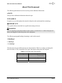

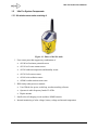
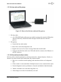

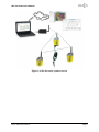
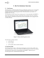
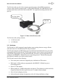
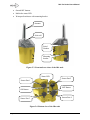
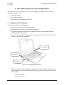
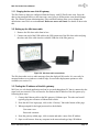
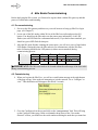
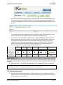
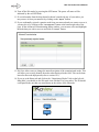
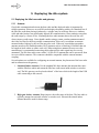
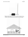
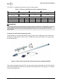
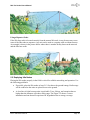
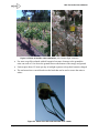
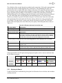

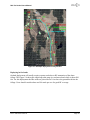

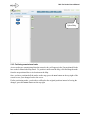


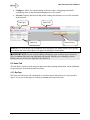
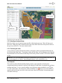
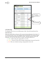
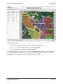


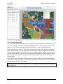
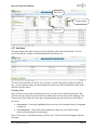
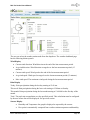
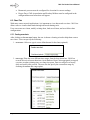
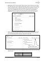
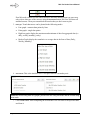
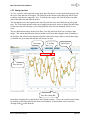
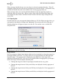
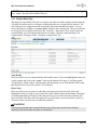

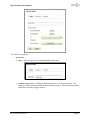
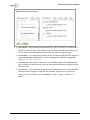
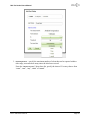
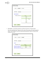
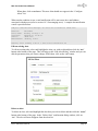
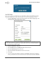
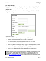
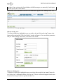
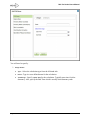
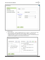


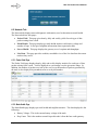
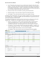
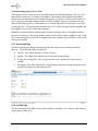
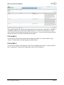
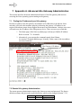
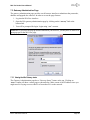
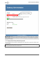

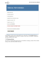
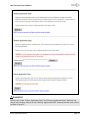
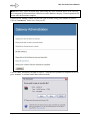
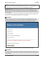
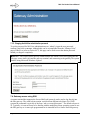
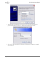
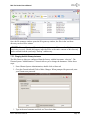
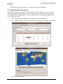
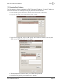
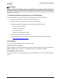
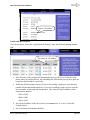

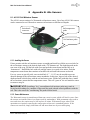
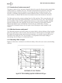
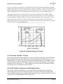
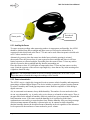

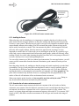
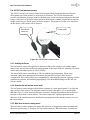
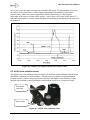
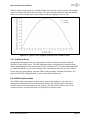
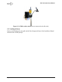
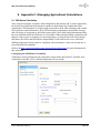
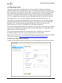
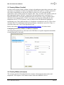
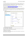




![CRM500GA-[] Installation Manual](http://vs1.manualzilla.com/store/data/006898113_1-6a3403dda4ef0cbf7e311a8a73ef8735-150x150.png)