Download A Novel, Web-Driven Continuous Mining

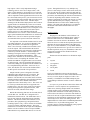
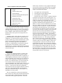
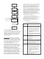
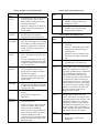
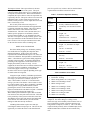
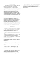
A Novel, Web-Driven Continuous Mining
Simulator
By
Steven J. Schafrik
and
Michael Karmis
Department of Mining and Minerals Engineering
Virginia Tech, Blacksburg, VA
and
Zacharias Agioutantis
Department of Minerals Resources Engineering
Technical University of Crete, Greece
ABSTRACT
The algorithms for the mathematical modeling to
predict productivity of underground room-and-pillar
mining systems are well known and documented. These
algorithms consider the time-varying relationships
between mining equipment for a given geometry of
operations as well as other constraints. This paper
presents WebConSim, a newly developed, Web-based,
user-friendly computer simulation tool for the Windows
environment. The simulator is easily customized for use
by field engineers, planning engineers, and management
and will help mine operators plan the optimum mining
sequence for different mine geometries and equipment
layouts. Program output includes production data and
equipment utilization indices, as well as time driven event
chains that can be used for virtual reality presentations.
INTRODUCTION
One of the main purposes of computer simulation is to
imitate the operations of real-life systems or processes.
The advantage of such simulations is that operational
scenarios can be tested and evaluated without the need or
use of actual experimentation. Since the early1960s,
applications have been developed to simulate the space
and time relationships between mining equipment, mainly
in connection with transport systems (Topuz et al., 1989;
Zhao and Suboleski, 1987; Ramachandran, 1983).
However, for the past ten years little work has been done
on modernizing the simulators by adapting them to the
new computing environments available and by allowing
for more complicated mining plans and extraction
procedures. Zhao and Suboleski (1987) give a detailed
account of the existing mine simulators at the time,
including CONSIM (Topuz et al., 1989), FACESIM
(Prelaz et al., 1968), and FRAPS (Haycocks et al., 1984)
developed at Virginia Tech, as well as UGMHS
developed at Penn State. Additionally, simulators with
graphics or animation capabilities, such as MPASS-2, are
also mentioned. SAM, the simulator developed by Zhao
(Zhao and Suboleski, 1987) can be added to this list as
well as FACEPROD, a simulator developed by Hollar
(Hollar, 2000). These dedicated simulation packages
were developed in general purpose programming
languages such as Fortran, Pascal, and Basic.
In addition to these simulation packages, programs
written in general purpose simulation languages, such as
GPSS, GPSS/H, Automod, and so forth (Vagenas, 1999;
Sturgul, 1999), have recently been applied toward the
development of discrete event simulation software
packages for both underground and open-pit mining
operations.
OBJECTIVES AND DESIGN OF THE NEW WEBBASED SIMULATOR
One of the most revolutionary advances in recent
years has been the wide proliferation of the client / server
architecture for collaborative software systems. The
Internet and company intranets supply the connectivity
for such applications. This new simulator (WebConSim)
was designed to use the power of the client / server
architecture, using current networking capabilities to
allow access to the simulator regardless of the type of
personal computer that the end user has. The actual
simulator resides on the server and the users can use any
kind of client to communicate their information to the
server (Figure 1). Suitable clients include any Internet
Explorer 3.0 compatible browser, including those running
under Microsoft Windows, Unix, and Apple Macintosh
operating systems, as well as browsers running on Palm
Pilots. Input data are stored in a database, which also
resides on the server. Therefore, a field engineer,
planning engineer, mine manager, and holding company
can all access the same information simultaneously. To
implement this design, three separate modules were
developed: the front-end module, the database module,
and the simulator module.
Web Browser
Client Side
Internet or Intranet
Web Server
Simulator
Database
Server Side
Figure 1. Simulator connectivity using a client / server
architecture
Front End Design
One of the benefits of using a Web-based front end is
that a client / server architecture can be utilized, where the
client communicates with the server by sending normal
http requests. This is easily implemented using a
technology such as Active Server Pages (ASP). ASP
allows a single database to be located on a server and all
Web content to be generated when the browser asks for it.
ASP is compatible with all popular Internet browsers that
have been made in the past five years because the browser
views normal Web content and all ASP processing occurs
on the server and not on the client. The other major
advantage to the Web-based deployment is that a software
upgrade needs to be installed only on the server location
and not on the clients. The simulator module can only be
hosted by a Microsoft Windows 9x or NT computer. This
computer must have Microsoft ActiveX Data Objects
(ADO) version 3.5 or later and Microsoft Internet
Information Services version 3 or later with Active Server
Pages option installed (Personal Web Server on Microsoft
Windows 9X). The server must be powerful enough to
accommodate all the expected concurrent connections.
It is important to note that the simulator itself is not an
executable application. It is an ActiveX Dynamic Link
Library (DLL) that is executed from an application.
There is no reason why a stand-alone executable could
not be developed. This would eliminate the need for
Internet Information Services and remove all the Internet
connectivity from the simulator. Another important
advantage of using the new ActiveX technology is that it
provides for encapsulation and inheritance. Thus,
changes to the simulator can be made without accessing
the source code or recompiling the simulator. This
includes the addition of equipment that is not accounted
for at design time. Once the operational logic has been
worked out, adding new equipment into the simulator can
be accomplished using inheritance. Each user can, in
effect, have his/her own version of the simulator that is
for their specific uses instead of for general uses.
Output from the system is designed to form both
traditional reports and time-driven event chains. The
traditional output includes cut numbers, times, and
distances. The time-driven event chains can be read into
animation packages and display the equipment operations
in real time. This is most valuable when used in
conjunction with a virtual reality viewer. The viewer can
be used to spot bottlenecks that are not apparent from
printed reports. Also, the viewer can be used for miner
training, showing how the equipment interacts, what
decisions are made, and when states change.
Besides the technology that runs the front end, there is
also the Web site. The Web site is designed to have
maintenance and action areas. The maintenance area is
how the user inputs the information into the simulator
database. This area has features that automate several
procedures, like equipment copy and paste functions
(reducing repetitive entry). These sections are an HTML
version of working with tabular datasets. The report
maintenance area contains all the output from simulations
that the user has not deleted. These are kept in HTML
tables that allow any standard Web browser to view the
reports. Through the Web site, every multiple-step
process is done using a wizard. In the action section, the
user can enter the cut sequence and travel paths and run
the simulation. Wizards take the user through these three
procedures, thus minimizing the amount of information to
be entered. Depending on the number of entries and
amount of equipment, the wizards can generate very large
(greater than 800 x 600 pixel) displays. Almost any
standard Web browser will be able to handle the large
displays. The main goal of the Web site is to minimize
the amount of data entered and maximize the user’s
throughput.
Database Design
The purpose of the database in this simulator is to
supply information to the simulation engine. Data are
stored in a Microsoft Access 2000 database, and the
simulator uses ADO to connect to the database. This
allows the user to override the development platform and
substitute the current implementation with a Microsoft
SQL Server, an Oracle database, or any ODBC database.
The goal of this abstraction is to give the user control over
the data acquisition. In any case, the database connection
string must be supplied to the simulator before the
simulation can begin.
The data stored in the database are divided into major
parts:
•
Layouts
•
Cut sequences
•
Waypoints
•
Travel paths
•
Teams
The layout information concerns only the physical
dimensions of the area to be mined. These dimensions do
not vary over time, depth, or length (see Table 1 for a
summary). The database can include multiple layouts
corresponding to different sections of a mine or different
mines.
Cut sequences govern the movement of the miners and
roof bolters. The cut sequences are repeated between
feeder moves, allowing multiple shifts to be simulated
without repetitive input. Information stored in the cut
sequence table includes the current mining location, the
next location to be mined, as well as the tram distance in
between for all cuts in a pattern. Both the miners and the
roof bolters use this information (summarized in Table 1)
when ready to move to the next mining location. This
implementation is similar to the CONSIM implementation
and allows for a very flexible mining pattern. Cut
sequences may be generated automatically (using separate
program modules) or keyed in manually.
Table 1. Mine Information Summary
Layout
Cut
Sequences
•
Entry and break widths
•
Floor, coal, and roof densities
•
Floor, coal, and roof heights
•
Number of entries
•
Cut number
•
Miner assigned
•
Roof bolter assigned
•
•
simulator is told what team to use, it is able to get all the
equipment by querying the equipment tables for the
appropriate team identifier. The nature of this filter-style
data storage abolishes the need to have several one-tomany relationships. These types of relationships are not
available to all potential database sources and are
computationally expensive.
Table 2. Equipment Information Summary
•
Length
Waypoint area
•
Time to begin a break cut
Next waypoint area
•
Tram rate profile
•
Load rate profile
•
Cutting rate profile
•
Miner storage capacity
•
Initial location and state
•
Mean time between failures
•
Mean time to repair
•
Statistics type
•
Length
•
Bolting rate (linear ft./minute) profile,
either constant or variable by entry
•
Tram rate profile
•
Initial location and state
•
Mean time between failures
•
Mean time to repair
•
Statistics type
•
Number of ways (one, two, three)
•
Capacity
•
Time to relocate
•
Minimum and maximum number of
breaks outby face
•
Processing rate profile
•
Distance inby center line of break
•
Initial location and state
•
Mean time between failures
•
Mean time to repair
•
Statistics type
The physical movements and location of all
equipment are based on waypoints. A waypoint is defined
as the center point at each entry / crosscut intersection.
The simulator calculates the location and coordinates of
each waypoint by taking the upper left corner at the
maximum number of breaks inby the feeder. Then the
waypoint numbers are arrayed to the right and down.
They are points of travel as well as reference points for all
mobile equipment. When these points are generated, the
inby, outby, left, and right neighbor relationships are also
calculated. Also, these points keep track of how much
material is scheduled to be mined and/or has been mined
in each of these directions. The same information is kept
regarding the length of the bolted entry in each direction.
In summary, the calculation of all physical locations of
moving equipment is based on the waypoints. The
waypoints are not stored in the database but are generated
in each simulation run based on the layout information.
Travel paths are critical to the overall effectiveness of
the system. The database stores the travel paths as
defined with reference to waypoints. The distance and
number of turns is a property of the path. For any single
to-and-from pair, there must be more than one entry in the
paths section of the database, unless only one piece of
equipment can travel between the two points at any given
time. For instance, if a shuttle car has been loaded by a
miner at waypoint 5 and would like to tram to the feeder
located at waypoint 14, it must look for an available path
entry from 5 to 14. Then the simulator calculates the
amount of time to make the journey.
Teams are mining crews and may include any
combination of mining equipment. This section of the
database is the most complicated, and its design is based
on the FACEPROD interface. The design is intended to
reduce the query time and complexity, while allowing
information to be easily duplicated while the user is
compiling a team. This is accomplished within one table.
The team’s table stores only two pieces of information, a
team identifier and a name. Each equipment type that is
handled by WebConSim has a table in the database. This
table stores a variety of information, as summarized in
Table 2. What is most important in the actual information
stored is the team identifier. This way, when the
Miner
Roof
Bolter
Feeder
breaker
Table 2. Equipment Information Summary
Shuttle
Car
makes it truly event driven. Every equipment unit keeps
its own Time to Next Event (TNE), the time to complete
the current task and reevaluate its state. The simulation
engine is interested in three things:
•
Capacity
•
Length
•
Switch in and out times
•
the original state of the equipment,
•
Turnaround time
•
the final location of the equipment, and
•
Tram rate unloaded and loaded profiles
•
•
Discharge rate profile
•
Turning rate profile
•
Initial location and state
•
Mean time between failures
•
Mean time to repair
•
Statistics type
Storage of teams in this manner increases the ease of
copying equipment from one team to another. The front
end allows this functionality very easily. It also allows a
new team member to be based on an existing equipment
piece or template. Entire teams can also be copied
quickly because of the speed of accessing all the team
information.
In addition, Table 2 shows that there are many pieces
of information that are not unique to a specific piece of
equipment (e.g., mean time between failures, mean time
to repair, statistics type, location, and initial state). These
data are critical for all equipment for the simulator to
operate. The statistics type can be deterministic or
stochastic, as explained below, and is directly related to
the rate profile of the equipment. The rate profile
includes the rate’s average, standard deviation, minimum,
and maximum and need store only the proper data for the
chosen statistics type.
Simulator Design
In most of the dedicated simulators available today,
the simulator is designed based on a specific scenario
regarding types and operational models of equipment, as
well as equipment restrictions. However, this approach
limits the simulator to the scenario types for which it was
created. These simulators are limited to the same basic
premise: one continuous miner, one to three shuttle cars,
one roof bolter, and one feeder (Zhao and Suboleski,
1987; Ramachandran, 1983; Hollar, 2000). However, this
specific scenario does not keep up with current mining
practices. At the same time, they do not implement
collision detection between equipment that may share the
same route. These limitations have forced engineers
doing time and machine analysis to develop their own
spreadsheets or work by hand.
The new simulator does not have these limitations.
This is because the design of the simulator implements an
expert system engine, in which the focus is not on the
scenario but on the equipment operations. This focus
the capabilities of the equipment.
From these three pieces of data, a complete simulation
to and from any time point can be accurately done. It is
important to note that the programming technology used
in this new simulator was not available to previous
simulator elements. More specifically, this expert system
approach is implemented using equipment states. A
shuttle car, miner, roof bolter, and feeder have states that
they are in. While in a state, there is a time that the piece
of equipment will be in that state. Its TNE is the current
time plus the current operation time. Once a state has
been completed, the equipment operator must decide what
to do next. This decision is a function of the current state,
the time in the current state, and what the next job is.
Therefore, any kind of equipment can easily be added by
allowing for appropriate state changes. The simulator
operates as shown in Figure 2. It is important to note that
the actual simulator does nothing except set a global time
and find the next time to set. The setting of the global
time is where the processing is actually done. When the
time is set on a piece of equipment, the equipment checks
whether its TNE (or time to state change) is equal to the
current global time. If the times are the same, then the
equipment decides what its new current state is and how
long it will be in this state. Once this has been completed
for all equipment, the simulator engine will “ask” each
piece of equipment for its TNE, then it will calculate the
minimum of these values and use that as the new global
time. This allows for multiple pieces of equipment to be
running different activities concurrently.
The normal distribution uses the average and the standard
deviation, while the exponential distribution uses the
mean rate. User-defined analysis allows the user to create
ranges of values based on a range of probabilities (e.g.,
from 0% to 25% is 3, from 26% to 75% is 5, 76% to
100% is 10). While determining the TNE, each piece of
equipment will use the statistical analysis for the specific
operation. For example, the tram rate is an input variable
for most equipment, where the product of the tram
distance and the tram rate yields the time to complete a
tramming operation. The tram rate in the above
relationship will be determined based on the statistics set
for the specific piece of equipment.
Begin simulation
Increment global
time
Set time on all
equipment
Process State
Changes
Report Collector
loop
Find minimum TNE that
will become the new global
time
The breakdown times and operating times are
calculated based on the mean time between failures and
mean time to repair. These are assumed to be
exponentially distributed because they are interarrival
times. This cannot be overridden using the current
version of WebConSim.
Table 3. Roof Bolter State Change Logic
Done?
Current
State
Action
Bolting
•
Determine next place to be bolted.
•
If that place is still occupied by the
miner, then change state to waiting.
Set the TNE equal to the miner’s TNE.
•
If that place is still occupied by
another bolter, then determine the next
available place.
•
When a place to bolt is found, set the
TNE to the product of distance and the
tram rate.
•
Set the roof bolter state to the state
before broken.
•
Reset TNE to account for the
breakdown.
•
Set roof bolter state to bolting.
•
Calculate TNE based on the product of
the amount that’s been cut and the
bolting rate for this entry.
•
Determine next place to be bolted.
•
If that place is still occupied by the
miner then change state to waiting.
Set the TNE equal to the miner’s TNE.
•
If that place is still occupied by
another bolter, then determine the next
available place based on the cut
sequence.
•
When a place to bolt is found, set the
TNE to the product of distance to the
place and tram rate.
End Simulation
Format Reports
Figure 2. Flow of Simulation
The type of simulation described is a new approach.
It uses relatively new programming technologies to allow
for multiple smart objects to be located in an artificially
confined area. Each object decides on the optimum way
to follow the plan that is set by the user, and then it
executes that procedure.
Simulation Logic: Simulation logic is evaluated when
state changes occur. The state changes occur when the
TNE for the equipment is equal to the current simulation
time. The logic then will set the new state, the new TNE,
and the physical changes that occur during the current
state. The simulator logic regarding the equipment is
shown in Table 3 through Table 6.
Each equipment parameter (i.e., tramming rate,
breakdown rate, etc.) can be evaluated based on statistical
information available for the specific piece of equipment
Thus, equipment parameters can be estimated either
deterministically or stochastically. Stochastic
distributions currently support the normal distribution
(e.g., for tramming rates), the exponential distribution (for
breakdowns and repairs), the uniform distribution, and
user-defined distributions, where the user can enter a
measured cumulative distribution function in a table form
to be used by the simulator. The deterministic analysis
uses only an average for the variable. The uniform
analysis uses an upper and lower bound for the variable.
Broken
Tramming
Waiting
Table 5. Feeder State Change Logic
Table 4. Shuttle Car State Change Logic
Current
State
Tramming
to Miner
Action
•
•
If the miner area is clear or the current
location equals the miner’s, then
change state to waiting to be loaded.
Set TNE to the miner’s.
Otherwise, change state to waiting to
switch-in and set the TNE equal to
switch-in time.
Tramming
to Feeder
•
Change state to unloading.
•
Set TNE equal to the product of
dumping rate and the current load.
Waiting to
be Loaded
•
If the miner area is clear or we are at
the miner, then change state to waiting
to be loaded. Set TNE to the miner’s.
Done Being
Loaded
Operating
•
Change feeder state to broken.
•
Calculate TNE using the feeder’s
mean time to repair.
•
Change feeder state to operating.
•
Calculate TNE using the feeder’s
mean time between failures.
Broken
Table 6. Miner State Change Logic
Current
State
Action
Cutting
•
Check whether the cut has been
completed
Otherwise, change state to waiting to
switch-in and set the TNE equal to
switch-in time.
•
•
Notice this is 100% controlled by the
miner. The shuttle car doesn’t ever set
this state.
If the cut is completed, then set state to
waiting to tram and set the TNE to
essentially zero.
•
•
Set state to tramming to feeder. Look
up the distance and profile of the path
to find the amount of time it will take;
use this for the TNE
Otherwise, switch to waiting to load
and set the TNE equal to essentially
zero.
•
Set state to waiting to load.
If the miner area is clear or the current
location equals the miner’s, then
change state to waiting to be loaded.
Set TNE to the miner’s.
•
Otherwise, change state to waiting to
switch-in and set TNE equal to the
switch-in time.
Done
Unloading
•
Set state to tramming to miner. Look
up the distance and profile of the path
to find the amount of time it will take.
Use this for the TNE.
Broken
•
Set shuttle car state to the state before
broken.
•
Reset TNE to account for the
breakdown.
•
Determine whether the feeder can
accept this shuttle car.
•
If there is not space, then set the TNE
equal to the smallest TNE of all the
shuttle cars that are unloading.
•
If the feeder can accept this shuttle car,
then set the TNE equal to the current
load x the dumping rate (this is
worked out between the feeder and the
shuttle car based on the feeder’s rate
and current load)
Waiting at
the Feeder
Action
•
•
Waiting to
Switch-in
Current
State
Tramming
Waiting to
Load
Waiting to
Tram
Broken
• Set TNE equal to essentially zero.
First, make sure another miner isn’t cutting
in the air split. If one is, then set the TNE
equal to the cutting miner’s. Otherwise,
start cutting, providing there is a shuttle car
that is located at the same place and
waiting to be loaded. If all that is true,
then compare the capacity of the shuttle car
to the amount of coal left in the cut and
invert the least to linear feet. Calculate the
TNE by taking this value times the cutting
rate. However, if there is nothing waiting
and there is no load, then the miner will
take a cut to load the miner (precut).
Change the state to cutting.
The miner looks at the cutting sequence to
find where the next place to be cut is
located. It also figures out what direction
needs to be mined (up, left, or right). Is the
destination occupied? If it is occupied,
then switch to waiting to tram and set the
TNE equal to the equipment in the way. If
the place is empty, then get the distance to
the place from the cut sequence and set the
TNE equal to the tram rate x distance.
•
Set miner state to the state before
broken.
•
Reset TNE to account for the
breakdown
The Report Collector: The report collector is the most
memory-intensive operator in the system. The report
collector monitors all the states of every equipment piece
at all points in simulation time. When each simulation is
completed, the report collector creates the report that was
requested by the user. The report collector can create both
traditional reports, in other words, those based on cut
numbers or time period, as well as output that can be read
into a virtual reality viewer.
This is easily achieved because each piece of
information that is collected includes the equipment that
is reporting it and the state change. The report collector
indexes each of these entries based on the current
simulation time. The mine’s state (amount mined, etc.)
and the specific equipment’s accumulators (distance
traveled, amount loaded, etc.) are included in the entry.
The time or cut reports are simple summary queries. The
time report summarizes all the information based on the
time it occurred. The cut report summarizes these data
for the time between the miner’s tramming state.
place for a specific cut, in either a brief or detailed format.
A generalized event chain is shown in Table 8.
Table 7. Verification Input Data Summary
Input
Variable
Data
Mine
Physical
Properties
•
Pillars 60' x 60'
•
20' entry width and break width
•
Coal density of 0.042 tons/ft2 and 60"
high
Shuttle
Cars
•
Two shuttle cars
•
Length – 28'
•
Capacity – 6 tons
•
Loaded tram rate – 300 ft/min
•
Unloaded tram rate – 450 ft/min
•
One miner
•
Length – 32', maximum cut depth –
19' ± 1'
•
Cut rate – 10 tons/min
•
Tram rate – 66 ft/sec
•
One feeder
•
Two-way
•
Load rate – 20 tons/min
•
One roof bolter
•
Length – 30'
•
Tram rate – 100 ft/sec
•
Bolting rate – 0.5 linear ft./min
Miner
SIMULATOR VALIDATION
The WebConSim package was validated by running
case studies that were originally developed for other
dedicated simulators. In this respect, the example
reported in the CONSIM manual (Topuz et al., 1989) was
selected for validation. The input data are summarized in
Table 7. These data are typical of the mining equipment
available in the early1980s. All statistical information
pertaining to this equipment is omitted from Table 7, to
simplify the summary of the case study. For all
equipment, the mean time between failures and mean time
to repair is required. In addition, as noted above, the
lower bound, upper bound, average, and standard
deviation of the rates are required, depending on the type
of statistics that are being used.
Using these input variables, CONSIM reports that the
first cut has an average mining rate of 2.45 tons/min and
an average cycle time of 41.1 minutes (Topuz et al.,
1989). WebConSim’s results are 2.3 tons/min and an
average cycle time of 45 minutes. These results are close
to, but do not match exactly, those produced by CONSIM.
Allowing for the varying random numbers used for
generating the statistics in the simulations, the most
important consideration is the shuttle car paths. CONSIM
has a single path for both of the shuttle cars.
WebConSim’s path mechanism requires that two shuttle
cars cannot use the same path at the same time. This adds
to the practicality of the system but also takes more time.
The addition of travel time will decrease the amount that
can be mined. Note that both the cycle time and the
mining rate both increased by around 9%.
Validating WebConSim requires more than just
examining the numerical output per cut. The user has the
opportunity to examine the actual event chain that took
Feeder
Roof Bolter
Table 8. Simulator Event Chain
1.
2.
3.
4.
5.
6.
7.
8.
9.
10.
Feeder operating
Roof bolter 1 bolting
Miner cutting/shuttle car 1 being loaded
Shuttle car 2 unloading at feeder
Miner waiting to load
Shuttle car 1 tramming to feeder
Shuttle car 2 tramming to miner
Shuttle car 2 waiting to be loaded
Shuttle car 1 waiting at feeder
Shuttle car 1 unloading
This general sequence is repeated until the cut is
completed. The miner changes to waiting to tram,
follows the logic, and eventually will tram to the next cut.
The roof bolter has a similar event chain when the area
being bolted is complete (see Table 3). The event chain,
coupled with the proximity to the CONSIM output, shows
that WebConSim does simulate the environment fairly
well.
CONCLUSIONS
WebConSim is a new type of simulator, which is not
built for just a single scenario, but which can
accommodate the majority of scenarios found in
contemporary continuous miner sections. The simulation
engine is an expert system that evaluates the system’s
state when events on each system participant are
completed. These decisions are based on the physical
characteristics of the system at the time it is being
evaluated (detailed in Table 3 through Table 6). This
simulation gathers its data from a database. The data are
accessible via the data-driven Web site (back end). This
same information can be made available to different users
that have access to the same network, which can be the
Internet or a company intranet. The back end needs to be
running on a desktop computer using an operating system
using Microsoft's Windows 9x or Windows NT
technology. The end user can be any type of computer
that has access to the network and uses an Internet
browser that is Microsoft Internet Explorer 3.0
compatible. WebConSim does generate similar results to
existing continuous miner simulators. These results take
into account information that was not taken into account
in earlier simulators, and results differ less than 10%.
REFERENCES
Haycocks, C., Kumar, A., Unal, A., Osei-Agyemana,
S., 1984, “Interactive Simulation for Room and Pillar
Miners,” 18th APCOM, Institute of Mining and
Metallurgy, London, England, pp. 5591-97.
Hollar, P., 2000, personal communication, February
2000.
Prelaz, L., Bucklen, E., Suboleski, S., Lucas, R., 1968,
“Computer Applications in Underground Mining
Systems,” Vol. 1, R & D Report No. 37, Office of Coal
Research, Washington, D.C.
Ramachandran, D., 1983, “A Simulation Model for
Continuous Mining Systems,” M.S. Thesis, VPI & SU,
Blacksburg, Va.
Sturgul, J. R., 1999, “Discrete Mine System Simulation
in the United States,” International Journal of Surface
Mining, Reclamation, and Environment, Vol. 13, pp. 3741.
Topuz, E., Nasuf, E., Ramachandran, D., 1989,
“Consim: An Interactive Micro-computer Program for
Continuous Mining Systems,” User Manual, 2nd
Revision.
Vagenas, N., 1999, “Applications of Discrete-Event
Simulation in Canadian Mining Operations in the
Nineties,” International Journal of Surface Mining,
Reclamation and Environment, Vol. 13, pp. 77-78.
Zhao, R., Suboleski, S., 1987, “Graphical Simulation of
Continuous Miner Production Systems,” APCOM 87:
Proceedings of the 12th International Symposium on the
Application of Computers and Mathematics in the
Mineral Industry.