1
Ecological Archives E091-067-A4
O. Gimenez and R. Choquet. 2010. Individual heterogeneity in studies on
marked animals using numerical integration: capture–recapture mixed
models. Ecology 91:951–957.
Appendix D: Incorporating individual random effects using program E–SURGE
In this appendix, we provide a step-by-step procedure to fit model {φ(x + x2 + x3 + h), p}
that was used in the Sociable weaver case study using numerical integration as implemented
in program E–SURGE. E–SURGE is available from http://www.cefe.cnrs.fr/BIOM/logiciels.htm,
and is described at length in Choquet et al. (2009) and in the E–SURGE user manual. The
implementation of capture–recapture mixed models in E–SURGE is also described in Choquet and Gimenez (2010).
1
Read in data
E–SURGE accepts capture–recapture (CR) data either in MARK or BIOMECO format.
The two types of data file are not very different: each row corresponds to a particular capture
history followed by the number of individuals with that history. In MARK format this count
is followed by a semi-colon and in BIOMECO format the data are preceded by the number
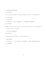
of different capture histories and the number. Below are the CR histories of the 6 first
individuals of the data set we considered in the Sociable weaver case study (MARK format),
the last three columns being standardized body mass, squared body mass and body mass
raised to the power three.
10000000 1 -0.8305 -0.2190 0.0969;
11100000 1
0.7385 -0.2086 -0.0545;
11100000 1 -1.8007 1.1382 0.8611;
2
11100000 1 -0.2436 -0.5342 0.0241;
11000000 1
0.6307 -0.2965 -0.0269;
11000000 1
0.6426 -0.2874 -0.0296;
From E–SURGE, start a new session named ”result.mod” from pull-down menu ”Start”.
Read in the data file (from ”Data” menu) and specify in E-SURGE that there are three
individual covariates when the question ”Is there external variables” pops up.
Amend the number of capture occasions, groups and age classes if needed: here we have
8 capture occasions, 1 age class and 1 group (use ”Modify” button in the ”Data Status”
panel). Now because we work in a multi–event framework (Pradel, 2005) we need to define
the events and states: we consider a standard Cormack-Jolly-Seber-type (CJS) model, which
is easily obtained by using 2 events – non detection or detection – and 2 states – alive or
dead. By default, E–SURGE gets it right here.
2
Fitting the model
Fitting a model in E–SURGE involves four steps:
• The GEPAT step: specifying which ones of all the potential parameters have to be
estimated, which ones will be calculated as the complement to 1 and which ones correspond to impossible events or transitions and are fixed to zero;
• The GEMACO step: specifying effects (time, age) acting on the parameters;
3
• The IVFV step: specifying initial values for the optimization procedure and / or fixed
values for the active parameters;
• The RUN step: launching the optimization procedure.
2.1
Specifying the pattern matrices using the GEPAT interface
There are three types of parameters used in the definition of a multi–event model (Pradel,
2005):
• The initial state probabilities Π;
• The transition probabilities Φ make the link between states at time t given states at
time t − 1;
• The event probabilities B make the link between events at time t and states at time t.
To enter the GEPAT interface, click the GEPAT button at the bottom of the main
window. By default, E–SURGE leaves all live states available as initial steps. The state
dead, last in the list, is impossible and does not appear. The last live step is taken by
default to be the one whose probability will be calculated indirectly, as the complement of
those of the other live states. This is specified using the following general conventions for
GEPAT:
• A minus sign (-) indicates that a potential parameter is unavailable in the current
model (impossible transition for instance). This is equivalent to fixing it to zero but
more explicit;
4
• Any greek letter (strike a latin letter and E–SURGE will show its greek counterpart)
indicates a free parameter, one to be estimated directly. Note that the particular greek
letter entered is totally irrelevant to E–SURGE. In particular, the same greek letter
is used repeatedly by default within a pattern matrix; this does NOT mean that the
parameters are being forced to be equal;
• The asterisk (*) indicates the parameter that is calculated indirectly, as the complement
to 1 of all the other parameters on the same row. There MUST always be one and
only one asterisk per row.
Note that the order of the states is chosen by the user except for the dead state that is
always positioned last. Here, by default, the pattern proposed by E–SURGE is correct for
the model we want to fit, therefore press the EXIT button to leave the GEPAT interface.
The vector of initial state is
Π=
1 0
which gives in the GEPAT syntax
∗
.
In the Sociable weaver case study, because we have only two states, the transition matrix is
simple with only 1 parameter for survival to be estimated
φ 1−φ
Φ=
0
1
5
which gives in the GEPAT syntax
ψ ∗
− ∗
(the first column corresponds to the probability of being alive conditional on being alive or
dead at the previous occasion). For the event, we have also a single parameter to estimate
for detection
p 1−p
B=
0
1
which gives in the GEPAT syntax
∗ β
∗ −
(the second column corresponds to the probability of being detected conditional on being
alive or dead).
2.2
Specifying the model using the GEMACO interface
The GEMACO interface uses keywords to create a modelling sentence that specifies how
parameters vary by time, over groups, over age classes, etc. At the end of the GEMACO
procedure, a design matrix is created for each type of parameters. Each row of the design
matrix will correspond to a parameter of the full model (all potential variability: time, age,
group) and each column corresponds to a parameter of the actual model. The GEMACO
syntax is fairly intuitive but the ”sentences” you enter in the GEMACO interface must
6
respect some priority rules that we will not develop here. We encourage the user to read
the E–SURGE user manual and Choquet (2008) in which the GEMACO syntax is fully
explained.
• Modelling the initial states
For the CJS model, the set of initial state probabilities is empty. Click on ”Initial
State” button on top of the panel to proceed to the ”Transition” window.
• Modelling the transition probabilities
To specify the model on transition probabilities, we used the keyword ”i” for the intercept, the keyword ”xind” for slopes corresponding to individual covariates and the
keyword ”ind” for an individual random effect. To combine them all, the GEMACO
sentence should be ”i + xind(1,2,3) + ind”. On top of the panel, click on the ”Transition” button to proceed to the ”Event” window.
• Modelling the event probabilities
Because the model conditions on the first capture occasion of each individual, the only
event to model at the time of the first encounter is the state of capture. It is only later
on that the event ”not encountered” becomes possible. Thus, the event probabilities at
the time of the first encounter must be treated separately. This is achieved through the
use of the keywords ”firste”, which stands for ”first encounter”, and ”nexte”, which
stands for ”next encounters”, respectively. The output of GEPAT is shown in the
”transitions pattern” subwindow at the bottom left. For each state (in row), there is
7
only one active event which is the capture on the relevant state, and the other possible
event taken as the complement is ”not encountered” (first column). At the time of
the first encounter, the capture is certain and the capture probabilities will all be set
to 1. At this stage, we cannot specify a fixed value, but we can specify that we need
just one parameter common to all states by keeping ”firste” by itself. Later, capture
probability will be constant. Thus, the complete sentence is ”firste+nexte”.
At this stage, to create the design matrices, we click on the GEMACO item in the top
menu and select the ”call GEMACO (all phrases)” submenu. Then, press the EXIT button
to return to the main window.
2.3
Specifying the initial and fixed values using the IVFV interface
In E-SURGE, the user can choose the way to generate the initial values of the optimization
procedure. They can be either ”constant”, ”randomly generated” or ”equal to the estimates
of a previously fitted model”. Once the type of initial values is chosen, the user can also fix
the values for some parameters using the IVFV interface. Press the IVFV button to enter
the interface.
• The initial states probabilities
In this case, there is no need to specify neither fixed values nor initial values (although
it might be worth trying several different initial values for the standard deviation of
the random effect). On top panel, click on the ”Initial State” button to proceed to the
”Transition” screen.
8
• The transition probabilities
There is no need to fix values for the transition probabilities so this screen can be left
in its default state. Click on the ”Transition” button to proceed to the ”Event” screen.
• The event probabilities
We can see here the different capture parameters appearing in the definition of the
model. The series of number indicate successively: the line in the event matrix (corresponding to the state), the column in the event matrix (corresponding to the event),
the capture occasion, the age class, the group, the step in the matrix decomposition of
the event matrix (here 1). Thus, the first parameter corresponds to the capture rate
at the first capture occasion for the first age class, i.e. time of first encounter (A=1).
This is the only parameter with A=1 because we have gathered all the capture rates
relative to the first encounter into a single parameter. This parameter needs to be
fixed to 1. We do this by entering the value 1 as ”Initial Value” and ticking the box
nearby. The other parameter correspond to the following capture rates (A=2); there
is no need to fix these parameters.
After all the fixed values have been specified, press the EXIT button.
2.4
Running the model
Before running the model, we tick the ”compute C-I (Hessian)” option in the ”Advanced
Numerical Options” panel to obtain confidence intervals of the parameters. We also need to
9
specify the method of numerical integration. Here, we go for the standard Gauss–Hermite
quadrature method. Click ”Modify” in the panel ”Advanced Numerical Options” and set to
0 for non-adaptive Gauss-Hermite in the 4th line, and specify 15 quadrature nodes in the
5th value for the order of integration. Note that the adaptive Gauss–Hermite quadrature is
also available by specifying 1 in the fourth line. The model is now ready to be fitted to the
data, press the RUN button.
3
Interpreting the outputs
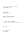
The output file (see next page) contains several pieces of information. The first paragraph
reminds you the characteristics of the data set, the second paragraph the GEMACO syntax
and the initial and fixed values, while the third and fourth paragraphs give numerical details.
The next paragraph tells us the number of estimable parameters: here we have 4 regression
parameters, 1 standard deviation for the distribution of the individual random effect, plus
1 detection parameter, therefore 6 parameters. We are also given the values of AIC and
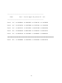
deviance. Finally, the parameter estimates are provided (on the scale of the link function),
together with standard errors and confidence intervals: beta1 is the intercept c0 , beta2, beta3
and beta4 are the regression parameters c1 , c2 and c3 , beta5 is the standard deviation of
the individual random effect, given on the scale of the square root. Using program R, we
back–transform to get the standard deviation by squaring the value E–SURGE, which gives
us
10
> 0.907975363*0.907975363
[1] 0.8244193
and we use the delta–method (resorting to the package ”msm”) to get its standard error
> library(msm)
> ?deltamethod
> deltamethod (~ x1*x1, 0.907975363 , 0.089961882*0.089961882)
[1] 0.1633663
Finally beta6 is the detection probability on the logit scale, which needs to be back-transformed
to obtain the detection probability
> 1/(1+exp(0.292820001))
[1] 0.4273136
and again use the delta–method to obtain its standard error
> library(msm)
> deltamethod (~ 1 / (1+exp(-x1)),-0.292820001 , 0.095215528*0.095215528)
[1] 0.02330083
11
OUTPUT FILE : C:\OG\...\phi(x1+x2+x3+RE) avec CI.out
Data File :C:\OG\...\weavers.inp
Number of occasions :
8
Number of states :
2
Number of events :
2
Number of groups :
1
Number of age classes :
1
---------------------------------------------Model Name : phi(x1+x2+x3+RE) avec CI
Model formula (or file) :
For Initial State:IS - Step 1 - (0):
For Transition:T - Step 1 - (5): i+xind(1,2,3)+ind
For Event:E - Step 1 - (2): firste+nexte
Init(values) 0.135152,0.250624,0.826779,0.917867,0.485031,0.913677,
Init(indices) 1,
3,
4,
5,
6,
7,
Fix(values) 1.000000,
Fix(indices) 2,
---------------------------------------------Link function : logitgen
Explicit gradient : off
TOLF : 0.000001
12
TOLX : 0.000010
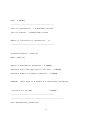
---------------------------------------------Time for optimisation : 2.912564e+002 seconds
Time for Hessian : 3.266891e+002 seconds
Number of iterations for optimisation : 17
----------------------------------------------
dev(PI)+dev(PHI,B) = 2376.181
QAIC = 2388.181
Number of mathematical parameters : 6.000000
Estimated model rank applicable to the data : 6.000000
Estimated number of boundary parameters : 0.000000
WARNING : there might be 0 further non identifiable parameters
c hat used for the QAIC
: 1.000000
-----------------------------------------------------------------------------------------------------Beta (Mathematical parameters)
13
--------------------------------------------------------Index
Beta | Lower & Upper 95 percent CI | S.E.
--------------------------------------------------------Beta#
1# | +0.509340913 +0.280820455 +0.737861371 +0.116592070
Beta#
2# | +0.015738742 -0.241075099 +0.272552582 +0.131027470
Beta#
3# | -0.268172515 -0.441169542 -0.095175489 +0.088263789
Beta#
4# | +0.081036919 -0.005817684 +0.167891522 +0.044313573
Beta#
5# | +0.907975363 +0.731650075 +1.084300651 +0.089961882
#########################################################################
Beta#
6# | -0.292820001 -0.479442436 -0.106197567 +0.095215528
14
References
Choquet, R. 2008. Automatic generation of multistate capture recapture models. The Canadian Journal of Statistics, 36:4357.
Choquet, R. and O. Gimenez. 2010. Towards built-in capture-recapture mixed models in
program E-SURGE. Journal of Ornithology.
Choquet, R., L. Rouan, and R. Pradel. 2009. Program E-SURGE: a software application for
fitting multievent models. In D. L. Thomson, E. G. Cooch, and M. J. Conroy, editors, Modeling Demographic Processes in Marked Populations, pages 845865. Series: Environmental
and Ecological Statistics, Vol. 3.
Pradel, R. 2005. Multievent : an extension of capture-recapture models to uncertain states.
Biometrics, 61:442447.
15