Download ROCCC 2.0 User`s Manual

ROCCC 2.0 User’s Manual - Revision 0.6
February 9, 2011
1
Contents
1 Changes
1.1 Revision
1.2 Revision
1.3 Revision
1.4 Revision
1.5 Revision
1.6 Revision
1.7 Revision
1.8 Revision
1.9 Revision
1.10 Revision
1.11 Revision
1.12 Revision
1.13 Revision
1.14 Revision
1.15 Revision
0.6 Added Features .
0.6 Bug Fixes . . . . .
0.5.2 Added Features
0.5.2 Bug Fixes . . . .
0.5.1 Added Features
0.5.1 Bug Fixes . . . .
0.5 Added Features .
0.5 Bug Fixes . . . . .
0.4.2 Added Features
0.4.2 Bug Fixes . . . .
0.4.1 Added Features
0.4.1 Bug Fixes . . . .
0.4 Added Features .
0.4 Bug Fixes . . . . .
0.3 . . . . . . . . . . .
.
.
.
.
.
.
.
.
.
.
.
.
.
.
.
.
.
.
.
.
.
.
.
.
.
.
.
.
.
.
.
.
.
.
.
.
.
.
.
.
.
.
.
.
.
.
.
.
.
.
.
.
.
.
.
.
.
.
.
.
.
.
.
.
.
.
.
.
.
.
.
.
.
.
.
.
.
.
.
.
.
.
.
.
.
.
.
.
.
.
.
.
.
.
.
.
.
.
.
.
.
.
.
.
.
.
.
.
.
.
.
.
.
.
.
.
.
.
.
.
.
.
.
.
.
.
.
.
.
.
.
.
.
.
.
.
.
.
.
.
.
.
.
.
.
.
.
.
.
.
.
.
.
.
.
.
.
.
.
.
.
.
.
.
.
.
.
.
.
.
.
.
.
.
.
.
.
.
.
.
.
.
.
.
.
.
.
.
.
.
.
.
.
.
.
.
.
.
.
.
.
.
.
.
.
.
.
.
.
.
.
.
.
.
.
.
.
.
.
.
.
.
.
.
.
.
.
.
.
.
.
.
.
.
.
.
.
.
.
.
.
.
.
.
.
.
.
.
.
.
.
.
.
.
.
.
.
.
.
.
.
.
.
.
.
.
.
.
.
.
.
.
.
.
.
.
.
.
.
.
.
.
.
.
.
2 Installation
7
7
8
8
9
11
12
13
14
14
15
16
16
16
17
18
19
3 GUI
3.1 Installing The Plugin . . . . . . . . . .
3.2 Preparing the GUI for using ROCCC .
3.3 GUI Menu Overview . . . . . . . . . .
3.3.1 ROCCC Menu . . . . . . . . .
3.3.2 ROCCC Toolbar . . . . . . . .
3.3.3 ROCCC Context Menu . . . .
3.4 Loading the Example Files . . . . . .
3.5 IP Cores View . . . . . . . . . . . . .
3.6 Creating a New ROCCC Project . . .
3.7 Build to Hardware . . . . . . . . . . .
3.8 High Level Compiler Optimizations . .
3.8.1 System Specific Optimizations
3.8.2 Optimizations for both Systems
3.9 Add IPCores . . . . . . . . . . . . . .
3.10 Create New Module . . . . . . . . . .
3.11 Create New System . . . . . . . . . . .
3.12 Import Module . . . . . . . . . . . . .
3.13 Import System . . . . . . . . . . . . .
3.14 Intrinsics Manager . . . . . . . . . . .
3.15 Open ”roccc-library.h” . . . . . . . . .
3.16 Reset Compiler . . . . . . . . . . . . .
3.17 Testbench Generation . . . . . . . . .
3.18 Platform Generation . . . . . . . . . .
3.19 Updating . . . . . . . . . . . . . . . .
2
. . . . . . . .
. . . . . . . .
. . . . . . . .
. . . . . . . .
. . . . . . . .
. . . . . . . .
. . . . . . . .
. . . . . . . .
. . . . . . . .
. . . . . . . .
. . . . . . . .
. . . . . . . .
and Modules
. . . . . . . .
. . . . . . . .
. . . . . . . .
. . . . . . . .
. . . . . . . .
. . . . . . . .
. . . . . . . .
. . . . . . . .
. . . . . . . .
. . . . . . . .
. . . . . . . .
.
.
.
.
.
.
.
.
.
.
.
.
.
.
.
.
.
.
.
.
.
.
.
.
.
.
.
.
.
.
.
.
.
.
.
.
.
.
.
.
.
.
.
.
.
.
.
.
.
.
.
.
.
.
.
.
.
.
.
.
.
.
.
.
.
.
.
.
.
.
.
.
.
.
.
.
.
.
.
.
.
.
.
.
.
.
.
.
.
.
.
.
.
.
.
.
.
.
.
.
.
.
.
.
.
.
.
.
.
.
.
.
.
.
.
.
.
.
.
.
.
.
.
.
.
.
.
.
.
.
.
.
.
.
.
.
.
.
.
.
.
.
.
.
.
.
.
.
.
.
.
.
.
.
.
.
.
.
.
.
.
.
.
.
.
.
.
.
21
21
21
23
23
25
25
26
28
28
29
33
34
34
35
35
36
37
38
38
38
38
39
39
41
4 C Code Construction
4.1 General Code Guidelines . . . . . . . . . . . . . . . . .
4.1.1 Limitations . . . . . . . . . . . . . . . . . . . .
4.2 Module Code . . . . . . . . . . . . . . . . . . . . . . .
4.3 System Code . . . . . . . . . . . . . . . . . . . . . . .
4.3.1 Windows and Generated Addresses . . . . . . .
4.3.2 N-dimensional arrays . . . . . . . . . . . . . . .
4.3.3 Feedback detection . . . . . . . . . . . . . . . .
4.3.4 Summation reduction . . . . . . . . . . . . . .
4.4 Instantiating Modules . . . . . . . . . . . . . . . . . .
4.4.1 Inlining Modules . . . . . . . . . . . . . . . . .
4.5 Control Flow . . . . . . . . . . . . . . . . . . . . . . .
4.6 Legacy Code . . . . . . . . . . . . . . . . . . . . . . .
4.6.1 Legacy Module Code . . . . . . . . . . . . . . .
4.6.2 Legacy System Code . . . . . . . . . . . . . . .
4.7 Compiling . . . . . . . . . . . . . . . . . . . . . . . . .
4.8 Hardware Specific Optimizations . . . . . . . . . . . .
4.8.1 Specifying Bit Width . . . . . . . . . . . . . . .
4.8.2 Systolic Array Generation . . . . . . . . . . . .
4.8.3 Temporal Common Subexpression Elimination
4.8.4 Arithmetic Balancing . . . . . . . . . . . . . .
4.8.5 Copy Reduction . . . . . . . . . . . . . . . . .
4.8.6 Fanout Tree Generation . . . . . . . . . . . . .
4.8.7 Smart Buffers . . . . . . . . . . . . . . . . . . .
.
.
.
.
.
.
.
.
.
.
.
.
.
.
.
.
.
.
.
.
.
.
.
.
.
.
.
.
.
.
.
.
.
.
.
.
.
.
.
.
.
.
.
.
.
.
.
.
.
.
.
.
.
.
.
.
.
.
.
.
.
.
.
.
.
.
.
.
.
.
.
.
.
.
.
.
.
.
.
.
.
.
.
.
.
.
.
.
.
.
.
.
.
.
.
.
.
.
.
.
.
.
.
.
.
.
.
.
.
.
.
.
.
.
.
.
.
.
.
.
.
.
.
.
.
.
.
.
.
.
.
.
.
.
.
.
.
.
43
43
43
43
44
45
47
47
48
48
50
50
50
50
53
54
54
54
54
55
56
57
57
57
5 Interfacing With Generated Hardware
5.1 Port Descriptions . . . . . . . . . . . .
5.1.1 Default Ports . . . . . . . . . .
5.1.2 Input And Output Ports . . . .
5.2 Interfacing Protocols . . . . . . . . . .
5.2.1 Input Registers . . . . . . . . .
5.2.2 Input Streams . . . . . . . . .
5.2.3 Output Scalars . . . . . . . . .
5.2.4 Output Streams . . . . . . . .
5.2.5 Done . . . . . . . . . . . . . . .
5.2.6 Stall . . . . . . . . . . . . . . .
5.3 Memory Organization . . . . . . . . .
5.3.1 Input Streams . . . . . . . . .
5.3.2 Output Streams . . . . . . . .
5.3.3 Systolic Arrays . . . . . . . . .
5.4 Pipelining . . . . . . . . . . . . . . . .
5.5 Fanout Reduction . . . . . . . . . . . .
5.6 Intrinsics . . . . . . . . . . . . . . . .
.
.
.
.
.
.
.
.
.
.
.
.
.
.
.
.
.
.
.
.
.
.
.
.
.
.
.
.
.
.
.
.
.
.
.
.
.
.
.
.
.
.
.
.
.
.
.
.
.
.
.
.
.
.
.
.
.
.
.
.
.
.
.
.
.
.
.
.
.
.
.
.
.
.
.
.
.
.
.
.
.
.
.
.
.
.
.
.
.
.
.
.
.
.
.
.
.
.
.
.
.
.
60
60
60
61
64
64
64
66
67
67
68
68
68
69
69
70
71
71
3
.
.
.
.
.
.
.
.
.
.
.
.
.
.
.
.
.
.
.
.
.
.
.
.
.
.
.
.
.
.
.
.
.
.
.
.
.
.
.
.
.
.
.
.
.
.
.
.
.
.
.
.
.
.
.
.
.
.
.
.
.
.
.
.
.
.
.
.
.
.
.
.
.
.
.
.
.
.
.
.
.
.
.
.
.
.
.
.
.
.
.
.
.
.
.
.
.
.
.
.
.
.
.
.
.
.
.
.
.
.
.
.
.
.
.
.
.
.
.
.
.
.
.
.
.
.
.
.
.
.
.
.
.
.
.
.
.
.
.
.
.
.
.
.
.
.
.
.
.
.
.
.
.
6 Generated Specific Hardware Connections
76
6.1 Basic Assumptions . . . . . . . . . . . . . . . . . . . . . . . . . . 76
6.2 Values created by optimizations . . . . . . . . . . . . . . . . . . . 77
7 Examples Provided
80
7.1 Module Examples . . . . . . . . . . . . . . . . . . . . . . . . . . . 80
7.2 System Examples . . . . . . . . . . . . . . . . . . . . . . . . . . . 82
8 Troubleshooting
84
8.1 Hi-CIRRF Failure . . . . . . . . . . . . . . . . . . . . . . . . . . 84
8.2 Lo-CIRRF Failure . . . . . . . . . . . . . . . . . . . . . . . . . . 85
4
List of Figures
1
2
3
4
5
6
7
8
9
10
11
12
13
14
15
16
17
18
19
20
21
22
23
24
25
26
27
28
29
30
31
32
33
34
35
36
37
38
39
Copying the Plugins into Eclipse . . . . . . . . . . . . . . . . . .
ROCCC 2.0 Registration Window . . . . . . . . . . . . . . . . .
Location of the ROCCC 2.0 Preferences . . . . . . . . . . . . . .
The ROCCC Preferences Page . . . . . . . . . . . . . . . . . . .
ROCCC Menu Items . . . . . . . . . . . . . . . . . . . . . . . . .
ROCCC Toolbar . . . . . . . . . . . . . . . . . . . . . . . . . . .
ROCCC Context Menu . . . . . . . . . . . . . . . . . . . . . . .
Importing the Examples . . . . . . . . . . . . . . . . . . . . . . .
The ROCCCExamples Project . . . . . . . . . . . . . . . . . . .
IP Cores View . . . . . . . . . . . . . . . . . . . . . . . . . . . .
Creating a New Project . . . . . . . . . . . . . . . . . . . . . . .
High-Level Optimizations Page . . . . . . . . . . . . . . . . . . .
Low-Level Optimizations Page . . . . . . . . . . . . . . . . . . .
Basic Control of the Pipelining Phase . . . . . . . . . . . . . . .
Advanced Control of the Pipelining Phase . . . . . . . . . . . . .
Stream Accessing Management Page . . . . . . . . . . . . . . . .
Successful compilation . . . . . . . . . . . . . . . . . . . . . . . .
VHDL Subdirectory Created . . . . . . . . . . . . . . . . . . . .
Add Component Wizard . . . . . . . . . . . . . . . . . . . . . . .
New Module Wizard . . . . . . . . . . . . . . . . . . . . . . . . .
Module Skeleton Code for MACC . . . . . . . . . . . . . . . . . .
New System Wizard . . . . . . . . . . . . . . . . . . . . . . . . .
System Skeleton Code for WithinBounds . . . . . . . . . . . . . .
Intrinsics Manager . . . . . . . . . . . . . . . . . . . . . . . . . .
Testbench Generation . . . . . . . . . . . . . . . . . . . . . . . .
Generate a PCore . . . . . . . . . . . . . . . . . . . . . . . . . . .
Dependent Files Window . . . . . . . . . . . . . . . . . . . . . .
Generated PCore Folders . . . . . . . . . . . . . . . . . . . . . .
Check For Updates . . . . . . . . . . . . . . . . . . . . . . . . . .
(a) Module Code in C and (b) generated hardware . . . . . . . .
(a) Using a loop in module code and (b) resulting hardware . . .
(a) System Code in C and (b) generated hardware . . . . . . . .
Accessing a 3x3 Window . . . . . . . . . . . . . . . . . . . . . . .
A system with a three dimensional input and output stream . . .
(a) System Code That Contains Feedback and (b) Generated
Hardware . . . . . . . . . . . . . . . . . . . . . . . . . . . . . . .
System Code That Results in a Summation Reduction . . . . . .
(a) Code That Instantiates a Module, (b) the Generated Hardware, and (c) Generated Hardware After Inlining . . . . . . . . .
Boolean Select Control Flow. (a) In the original C, (b) in the
intermediate representation, and (c) in the generated hardware
datapath. . . . . . . . . . . . . . . . . . . . . . . . . . . . . . . .
Predicated Control Flow (A) in the original C, (B) in the intermediate representation, and (C) in the generated hardware. . . .
5
21
22
22
23
23
25
26
27
27
28
28
29
30
31
32
32
33
33
35
36
36
37
37
39
40
40
41
41
42
44
45
46
47
48
49
49
51
52
52
40
41
42
43
44
45
46
47
48
49
50
51
52
53
54
55
56
57
58
59
60
61
62
63
64
65
66
67
68
69
Legacy Module Code . . . . . . . . . . . . . . . . . . . . . . . . .
Declaring And Using A Twelve Bit Integer Type . . . . . . . . .
C Code To Generate A Systolic Array . . . . . . . . . . . . . . .
Block Diagram Of Max Filter System . . . . . . . . . . . . . . .
Block Diagram Of Max Filter System After TCSE . . . . . . . .
System Code That Accesses a 3x3 Window . . . . . . . . . . . .
3x3 Smart Buffer Sliding Along a 5x5 Memory . . . . . . . . . .
System Code That Reads From A Fifo . . . . . . . . . . . . . . .
Memory Fetches When Using A FIFO . . . . . . . . . . . . . . .
Timing Diagram Of A System With Both Input Scalars And
Input Streams . . . . . . . . . . . . . . . . . . . . . . . . . . . . .
Block Diagram Of A Generated Module . . . . . . . . . . . . . .
Block Diagram Of A Generated System . . . . . . . . . . . . . .
C Code That Writes To Three Locations In The Same Stream
Each Loop Iteration . . . . . . . . . . . . . . . . . . . . . . . . .
Block Diagram Of Generated Hardware For Code That Writes
To Three Locations Each Loop Iteration . . . . . . . . . . . . . .
Timing Diagram Of Module Use . . . . . . . . . . . . . . . . . .
Timing Diagram Of Generated Code Reading From A Stream
With Memory Addresses . . . . . . . . . . . . . . . . . . . . . . .
Timing Diagram Of Generated Code Reading From A Stream
With Multiple Outstanding Memory Requests . . . . . . . . . . .
Timing Diagram Of Generated Code Reading From A Stream
With Multiple Channels . . . . . . . . . . . . . . . . . . . . . . .
Timing Diagram of Output Streams . . . . . . . . . . . . . . . .
Timing Diagram Of The End Of A System’s Processing . . . . .
C Code For MaxFilterSystem Which Uses A 3x3 Window . . . .
Basic Dataflow . . . . . . . . . . . . . . . . . . . . . . . . . . . .
Medium Dataflow . . . . . . . . . . . . . . . . . . . . . . . . . . .
High fanout a) before registering and b) after registering . . . . .
Generated Systolic Array Hardware . . . . . . . . . . . . . . . . .
Theoretical Interface to a 32-bit Floating Point Divide IPCore .
Wrapper for the Theoretical 32-bit Floating Point Divide . . . .
System Code Sections Translated Into Hardware . . . . . . . . .
C Code That Infers Ports . . . . . . . . . . . . . . . . . . . . . .
Generated Ports . . . . . . . . . . . . . . . . . . . . . . . . . . .
6
53
55
55
56
56
58
58
58
59
61
62
63
63
64
64
65
66
66
67
68
69
70
71
72
73
74
75
76
77
78
1
Changes
The changes in revision 0.6 over revision 0.5.2 are the following:
1.1
Revision 0.6 Added Features
• High Level Optimizations: Input and output ports to modules may be
specified as individual parameters instead of passed in a struct.
• High Level Optimizations: Input and output streams, scalars, and feedback scalars can be specified as individual parameters to system code as
opposed to local variable declarations.
• High Level Optimizations: N-dimensional streams are now supported, previously we only supported up to 2-dimensional streams.
• High Level Optimizations: Dead code elimination revamped and implemented for modules and systems.
• High Level Optimizations: Inlining of individual or all module instantiations supported.
• High Level Optimizations: Reduction code performing a summation is
now identified and custom hardware is created with much greater potential
throughput.
• Hardware Generation: Input and output streams interface with the outside world through FIFOs implemented using cross-clock BRAMS.
• Hardware Generation: User controlled addition of registers along paths
that have high fanout added.
• Hardware Generation: Users may specify a maximum allowable fanout
for every generated hardware signal, after which a fanout tree will be
generated and pipelined.
• GUI: More intuitive interface to controlling pipelining added to better
allow the user to specify pipeline depth.
• GUI: Optimizations now have default values that can be user controlled.
• GUI: Added a registration page on start up to receive news on ROCCC
2.0.
• GUI: When compiling, syntax errors are detected immediately and the
optimizations page does not open
7
1.2
Revision 0.6 Bug Fixes
• High Level Optimizations: Ports declared in new style modules now correctly keep their order in module instantiations.
• High Level Optimizations: Feedback variables that were also results of
predication statements are now correctly identified as feedback variables.
• Hardware Generation: Names of variables that were intermittently lost on
compilation are now maintained.
• GUI: Having extraneous files in the project subdirectories no longer causes
problems.
• GUI: Generating a testbench for systems that have no streams no longer
asks for multiple tests sets for input and output scalars.
1.3
Revision 0.5.2 Added Features
• High Level Optimizations: Modules may be specified as redundant
• High Level Optimizations: Data that flows from redundant modules to
redundant modules will make the intermediate voters redundant.
• Hardware Generation: The user can now specify when registers should be
inserted into high-fanout operations.
• Hardware Generation: Pure feedback calls are no longer output scalars.
• Hardware Generation: Redundancy vote intrinsics supported in low end.
• Hardware Generation: The outer loop induction variable can now be used
as the only index into a single dimensional array.
• GUI: Added support for redundancy in the compile flags.
• GUI: Added a BRAM to BRAM interface generation for systems
• GUI: PCores not support multidimensional output streams
• GUI: Added a new ROCCC perspective that starts on new installs/
• GUI: Added a ROCCC welcome page for installs and updates.
• GUI: Added an ”Add Intrinsic” button in the intrinsic list viewer.
• GUI: Menu enhancements.
• GUI: Added a table for output stream info that allows control of the
number of output channels.
• GUI: Now can import the ROCCC examples through a single button or
automatically done when setting the distribution for the first time.
8
• GUI: IPCores view now highlights out of date modules.
• GUI: Better error checking and handling.
• GUI: IPCores table now displays ports much more quickly.
• GUI: Dependent files window now supports adding a netlist, hdl, and
wrapper for each necessary component.
• GUI: PCores will have better user side support when dealing with floating
point values.
• GUI: Users can now create a new project through the ROCCC menu with
one button.
• GUI lock messages are more informative.
• GUI: Adding a test case on testbenches for input or output scalars will
copy the previous set rather than having all blank spots for the test values
• GUI: IPCores view will restart itself after a compile or cancel if it is
showing the GUI locked message.
• GUI: IPCores view will no longer clear the ports table after compile. Any
changes in the shown ports after compile will automatically be updated.
• GUI: Testbenches now output a message when they are done computing
data.
1.4
Revision 0.5.2 Bug Fixes
• High Level Optimizations: Fixed multiplication by constant elimination
to only work in integers and not floating point values.
• High Level Optimizations: Updated if conversion to process until no
change occurs.
• High Level Optimizations: Updated constant propagation to change additions of negative values into subtracts and subtracts of negative numbers
into additions.
• High Level Optimizations: Fixed a bug where some constant propagation
identities were identified on the left side of binary expressions but not the
right.
• High Level Optimizations: Fixed constant array propagation to work with
floating point values.
• High Level Optimizations: Fixed a bug in constant propagation where the
unary expression of convert wasn’t handled correctly.
• High Level Optimizations: Fixed issue with fully unrolling loops.
9
• Hardware Generation: Fixed several issues that caused generated VHDL
to not be accepted by XST, including assert statements in the output
controller and a counter variable changed from an asynchronous statement
to a process.
• Hardware Generation: Fixed issue where feedback could be above the
height of the datapath, and where feedback VHDL could be generated
multiple time, resulting in compile failure.
• Hardware Generation: Fixed issue that caused casts from one type to
another resulted in a segmentation fault.
• Hardware Generation: Fixed issue where using input scalars as the for
loop end values on a long pipeline could result in very poor generated
frequency.
• Hardware Generation: Pipelining pass changed to finish as soon as there
is no change, which dramatically speeds up compilation time on large
examples.
• Hardware Generation: Fixed issue where 1-bit signals that were signextended were incorrectly output.
• Hardware Generation: Fixed issue when using testbench with non-32-bit
output streams.
• GUI: Fixed error when preferences were locked when opened from ’Incorrect Distribution Folder’ message.
• GUI: Fixed other action problems that occurred when dealing with components that started with lower case c.
• GUI: Fixed bug in PCore generation when using an .ngc file caused an
”incorrect file name” error.
• GUI: Updates are now only allowed if the user has write permissions in
the distribution.
• GUI: No longer creating components whose names are C reserved words
or ROCCC reserved words.
• GUI: Adding intrinsics that cast from different datatypes now have correct
port names.
• GUI: Fixed errors when calling ROCCC functions with no file opened in
the editor.
• GUI: Dependent files window corectly adds the necessary data to the
PCore files when using netlists.
10
• GUI: Compilation will not be done if the user does not have write permissions in the folder where the file is being compiled.
• GUI: Any running ROCCC builds are now canceled when Eclipse is closed.
• GUI: PCore generation will no longer accept dependent files with spaces
in their name.
• GUI: Fixed testbench error when dealing with 1 bit streams.
• GUI: No longer allow generation PCores or testbenches on components
compiled with a previous version of the GUI. This applies to the newly
added BRAM interface generation as well.
The changes in revision 0.5.1 over revision 0.5 are the following:
1.5
Revision 0.5.1 Added Features
• GUI: Data types are displayed in the IPCores view.
• GUI: All loop based flags are removed from the compiler flags for modules.
• GUI: All loops in modules are automatically fully unrolled, no flag needed.
• GUI: Testbenching and PCores now handle the new port structures.
• GUI: Testbenching for systems has been redone to support user specific
input and output data for streams.
• GUI: Improved file selection boxes so it starts the browsing in the specified
file location or in the component folders.
• GUI: Testbench values now conform to the datatype of the port, not the
way the value was wrote.
• High Level Optimizations: High level verification pass asserts out on more
incorrect code.
• High Level Optimizations: Updated constant propagation to work on comparisons between two constants
• High Level Optimizations: Improved the if conversion pass to support
more complex control flow with arbitrary if statements.
• High Level Optimizations: Added a pass to handle the upcasting and
downcasting of both floats and integers so they can be mixed in expressions.
• Hardware Generation: Systolic arrays may now be retimed
• Hardware Generation: Made constant names much more readable by embedding the value into the constant name.
11
• Hardware Generation: Added support for systems that do not output
streams, only scalars, and systems that do not have input streams, only
scalars.
• Hardware Generation: Added low level support for writing port dataTypes
to the database.
• Hardware Generation: Added stall signal to all generated code.
• Hardware Generation: Created different code for output streams and output registers.
• Hardware Generation: Added support for signed comparisons in VHDL
generation, which required package support.
1.6
Revision 0.5.1 Bug Fixes
• GUI: The term ”delay” has been replaced by ”latency”
• GUI: Fixed a bug when compiling a component that starts with lower case
”c”.
• GUI: Fixed a bug with adding intrinsics with the same name and multiple
bitsizes where the old intrinsic was not overwritten.
• GUI: Floating point values are now converted to the correct binary format
in testbenching.
• GUI: Fixed bug in PCore generation where using an ngc and a vhdl wrapper did not go through.
• GUI: PCore plugin is only allowed to run if its version matches the main
ROCCC plugin.
• GUI: Files names hi cirrf.c can no longer be compiled or created using the
GUI ”Create” button.
• High Level Optimizations: Restructured the hi-cirrf output pass to be
easier to maintain.
• High Level Optimizations: Fixed an off by one error that caused loop
unrolling to unroll the incorrect amount.
• High Level Optimizations: Fixed an error that caused the insertion of
copies in the hardware to not be performed, resulting in incorrect hardware
in some cases.
• Hardware Generation: Issues with extra copies being made in systolic
arrays, which caused output data to sometimes be wrong, has been fixed.
• Hardware Generation: Made 64-bit floating point constants work correctly.
12
• Hardware Generation: Fixed binary addition of temporary boolean values.
• Hardware Generation: Fixed sizing issues when intrinsics are created to
correctly use the size of the output of the intrinsic, and not the default
size.
• Hardware Generation: Fixed issue where doing a cast from float to int
caused an assert to be thrown.
• Hardware Generation: Floating point greater than or equal operator did
not work correctly, even with intrinsic in database. Fixed by correcting
misspelling in string.
• Hardware Generation: Updated stream handler to correctly deal with
different sized streams, and also added better asserts across all stream
input/output.
• Hardware Generation: Fixed issue where 1 dimensional streams using
outermost loop induction variable in a 2 loop system failed. Tentative fix
on input, better error message for output.
• Hardware Generation: Making copy of same size floating point variable
instantiated FP core. Fixed to just make copy if copying same sized float.
• Hardware Generation: The latch for the input scalars going to the inputController as endValues is no longer the outputReady of the input
Controller, and instead is a direct connection to the entity port, which
prevents deadlock.
• Hardware Generation: ”done” no longer goes high until inputReady has
gone high at least once, to prevent register endValues from incorrectly
triggering ”done” before being set.
• Hardware Generation: Systems that switch the order of offset variables in
array accesses now work correctly.
• Hardware Generation: Systems now wait for inputReady to be triggered
before reading from streams.
• Hardware Generation: Fixed issue where port names were incorrectly
mangled.
The changes in revision 0.5 over revision 0.4.2 are the following:
1.7
Revision 0.5 Added Features
• GUI: Support for handling multiple intrinsics added
• GUI: Generation of Testbenches is supported for modules and systems
13
• GUI: Generation of PCores for integration with Xilinx EDK for certain
modules and systems has been added
• GUI: Infrastructure for Automatic updating has been added
• C Level: Support for floating point comparison and conversion added
• C Level: Floating point constants are propagated correctly
• C Level: Infinite for loops are now supported and generate systems that
can continuously run
• Optimization: Copy propagation is performed correctly
• Optimization: An optimization for fully unrolling all loops has been added
• Optimization: Tree balancing on the generated hardware is now selectable
• Optimization: Copy retiming on the generated hardware is now selectable
1.8
Revision 0.5 Bug Fixes
• C Level: The float constant -0.0 is now correctly identified and supported
• Optimization: Copy propagation is appropriately called when compiling
• Optimization: Loop fusion works correctly with variable bounded loops
• Optimization: Fully unrolling a loop previous would not unroll loops with
more than 100000 iterations
• Optimization: The algorithm that determines feedback variables has been
improved to a more efficient algorithm.
1.9
Revision 0.4.2 Added Features
• Usability: Support for 64-bit Ubuntu Linux added.
• Usability: The database used to store available IP cores has been reorganized to more efficiently send data between the different phases of the
toolset.
• Hardware Generation: The generated VHDL has decoupled the address
generation and reading of data, enabling a user determined amount of
reads to be outstanding and a user determined amount of data to be read
every clock cycle.
• Hardware Generation: When performing arithmetic in hardware, maximum precision is maintained.
• Hardware Generation: Support for integer division of arbitrary size has
been added, providing that an appropriate core exists in the database.
14
• Hardware Generation: The generated VHDL is passed through a retiming
algorithm to combine instructions into the same pipeline stage, greatly
increasing the efficiency of the generated VHDL.
• Hardware Generation: The timing of reading from input streams has been
changed to achieve maximal throughput.
• Optimization: Systems that have loops fully unrolled now correctly transform unrolled array accesses into lower dimension array accesses and scalars,
resulting in a module if all loops have been fully unrolled.
• Optimization: Support for fully unrolling loops in modules has been added.
• Optimization: Temporal common subexpression elimination can now be
used in conjunction with other system level optimizations.
• GUI: The ports shown for any component in the IPCores view are now
the C names and not the ROCCC generated VHDL names
• GUI: The menu has been reorganized.
• GUI: All modules are automatically exported upon compilation and replace any previous version
• GUI: Added a ”Cancel Current Compile” button to the toolbar
• GUI: Added a ”Verify ROCCC Distribution” button on the preference
page.
• GUI: Added a timing info page to the compiler optimizations
• GUI: Added a help tab on the menu which has an option to open the
ROCCC webpage.
1.10
Revision 0.4.2 Bug Fixes
• Feedback detection of variables is handled correctly for system code both
with and without module instantiation.
• Systolic Array generation now functions correctly with module instantiations.
• User database redesigned for feedback-generated compilation possibilities.
• Deleting modules from the GUI works properly in all cases.
• The port labeling on the IPCores double click is now ordered correctly
• No longer outputs ”indirect jmp without *” during compilation on Mac
machines
15
• Fixed bug where Build was clicked and GUI asked if you would like to
save the file, but compilation would not be done.
• Fixed bug on new module or system that caused modules or systems to
not be added to the database on first build.
• When editing fields in the compiler optimizations, neighboring text no
longer turns white
• No longer can have more than one ROCCC build happening at the same
time in the GUI
• Fixed bug where changing the ROCCC distribution folder on the preferences did not use the new database until Eclipse was restarted
1.11
Revision 0.4.1 Added Features
• The algorithm for inserting pipeline register copies, which resulted in long
compile times, has been rewritten, dramatically reducing the compile time.
• Compiling a module multiple times will overwrite the version in the database.
Previously, the database version would have to be deleted first.
• The streaming interface has the added capability of allowing multiple
memory requests to be issued.
1.12
Revision 0.4.1 Bug Fixes
• A bug that generated incorrect VHDL whenever the float constant value
0 was used has been fixed.
• Extremely large concurrent VHDL statements have been reworked to reduce the size of the generated VHDL.
• Adding a component to the database using the GUI now works correctly.
• Previously, optimization files for systems or modules in the GUI would be
shared by all systems or modules with the same name. Now, code that
shares a name will have separate optimization files.
1.13
Revision 0.4 Added Features
The changes in revision 0.4 over revision 0.3 are the following:
• Mac OS X Leopard support added
• Eclipse plugin GUI to control compilation and interface with the IP database
• Increased control over available optimizations
• Variable bit width integers are now supported.
16
• Systolic Array generation is now supported.
• Temporal common subexpression elimination is now supported.
• Negative offsets are supported to access arrays in system code.
• Hardware interface timing for streams has been made consistent with
memory interface timing
• Changed naming scheme for controllers in systems to uniquely identify
generated code
• Names of ports in the generated VHDL are a function of the original C
name
• Added support for shifting operators in the C code
• Updated the install script to detect and handle errors better
• Reduced compile time on tested systems
• More detailed error reports added during compilation
• More examples provided
• Documentation updated.
1.14
Revision 0.4 Bug Fixes
• Fixed bug where irregular window accesses caused incorrect data to be
fetched
• Fixed bug where done signal was triggering too early, now it coincides
with the last output value
• Fixed bug where constants being passed to subcomponents did not function correctly
• Fixed bug where insert copy pass used massive amounts of unnecessary
memory
• Fixed bug where multiple different modules were not allowed in the same
C code.
• Fixed bug that causes multidimensional buffers to be generated incorrectly
• Fixed bug where the first element of input streams was skipped if not used
• Fixed bug where valid C identifiers could result in invalid VHDL identifiers
17
1.15
Revision 0.3
The changes in revision 0.3 over revision 0.2 are the following:
• Division is now supported for integer values through the use of a division
core.
• Two dimensional arrays are supported in system code.
• FFT and Variance Filter examples added.
• Generated files no longer have DF prefix.
• Sample templates for interfaces on the SGI-RASC blade on an Altix 4700
system and a Xilinx ML507 board (which has a Virtex 5 FX70T FPGA)
are included.
• Documentation has been updated.
18
2
Installation
Installation and execution of ROCCC has been tested on the following systems:
• 32-bit Ubuntu Linux
• 64-bit Ubuntu Linux
• 32-bit CentOS Linux
• 64-bit CentOS Linux
• 64-bit OpenSuse Linux
• Macintosh Snow Leopard
Other systems are not supported.
The installation requires gcc 3.4 or above with g++, flex, bison, autoconf,
patch, python, and Eclipse 3.5.1 or higher. When uncompressed, the ROCCC
distribution folder should have the following directories:
• Documentation
The location of this user manual and the developer’s manual.
• Examples
A directory to be imported into the Eclipse framework that contains all
of the example code.
• GUI
The location of the Eclipse plugin .jar files.
• Install
The default location where ROCCC will be installed.
• ReferenceFiles
A directory containing the files necessary for PCore generation.
• Scripts
This directory contains scripts used in the install process.
• tmp
This directory is used for temporary storage when compiling with ROCCC.
Also, the ROCCC distribution folder will contain the following files:
• InferredBRAMFifo.vhdl
A VHDL file that is necessary for synthesis and simulation of ROCCC
generated system code.
• ROCCChelper.vhdl
A VHDL file that is necessary for synthesis and simulation of ROCCC
generated code. This file will also be placed in every vhdl subdirectory
upon compilation.
19
• StreamHandler.vhdl
A VHDL file that is necessary for simulation of systems using the testbenches created from the GUI.
• roccc-library.h
A link to the local copy of the header file that contains declarations of all
available modules and IP.
• vhdlLibrary.sql3
A link to the local copy of the database used to store all available modules
and IP.
• warning.log
This file will contain all warnings and errors encountered during installation. If installation was successful, this file can be removed without
consequence.
In order to install ROCCC, run the bash script file ”rocccInstall.sh.” This
script will untar, compile, and initialize all of the packages necessary for ROCCC.
If your system is missing an essential element for the compilation of ROCCC
an error message will be displayed and ROCCC will not be installed.
The rocccInstall.sh script takes two optional parameters, -s and -l, which
specify where to install the source files and local files respectively. By default,
both locations are the install directory.
Included in this distribution are Eclipse plugins that controls access to all
of the ROCCC functionality. The plugins are located in the GUI directory and
you are responsible for moving the files into the appropriate plugin directory on
your system and removing any previously installed ROCCC plugins that may
exist.
If you experience any failures in the installation procedure, consult the troubleshooting section at the end of this document.
20
3
GUI
The ROCCC GUI is a plugin designed for the Eclipse IDE that works on both
Linux and Mac systems. The user must have at least Eclipse version 3.5.1
installed. ROCCC currently supports the C++ and Java versions of Eclipse.
Eclipse can be downloaded for free at www.eclipse.org.
The ROCCC GUI plugin is continually evolving and may function slightly
differently in future releases.
3.1
Installing The Plugin
Once you have downloaded and uncompressed Eclipse, open the resulting uncompressed eclipse folder. Inside of there, you should see a folder named plugins.
This is where we need to copy the ROCCC GUI plugins into as shown in Figure
1. Any previous versions of the ROCCC plugins must also be removed from
this directory. The ROCCC plugins are located inside the GUI folder of the
uncompressed ROCCC distribution folder.
Figure 1: Copying the Plugins into Eclipse
Once you have moved the ROCCC plugins into the plugins folders inside
eclipse, ROCCC should be ready to run on Eclipse. The first time you run
Eclipse with the ROCCC plugins installed, ROCCC will set up the perspective
best used for working with ROCCC. It will also open up a page welcoming you
to ROCCC 2.0 and asking if you would like to register for updates and news as
shown in Figure 2.
3.2
Preparing the GUI for using ROCCC
Before we can use the core functionally that is bundled with the GUI, the user
must first set the directory path to the ROCCC distribution folder. This can
be done by selecting ”Preferences” in the ROCCC menu tab at the top of the
program as in Figure 3.
21
Figure 2: ROCCC 2.0 Registration Window
Figure 3: Location of the ROCCC 2.0 Preferences
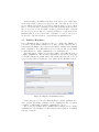
Once this is done, a preference page will pop up asking for the ROCCC
distribution path. Set the preference value to wherever you had uncompressed
the ROCCC distribution folder. The validity of the chosen folder can be checked
by clicking the ”Verify ROCCC Distribution Folder” button on the preference
page as shown in Figure 4.
Once that is done, the ROCCC GUI should be ready to use. If you ever
try to use any of the ROCCC functionality and this preference is not set or
that directory is incorrect, the GUI will tell you and ask if you want to set the
ROCCC distribution folder in the Preference menu.
22
Figure 4: The ROCCC Preferences Page
3.3
GUI Menu Overview
This is a quick overview of all the ROCCC buttons and options located on the
GUI for future reference. Each of the actions the buttons do will be covered in
more detail in the other sections, this is merely so you can see and recognize all
the buttons available.
Note: The icons on the menus may not show up if your system preferences
are set to not show Menu Icons.
3.3.1
ROCCC Menu
Figure 5: ROCCC Menu Items
23
•
Build: Compile the open modules or system file.
• New
– Project: Create a new ROCCC project in Eclipse.
– Module: Create starter code for a new ROCCC module.
– System: Create starter code for a new ROCCC system.
• Add
– IP Core: Add an IP Core directly to the database for future use.
• Import
– Module: Import an outside ROCCC module C file into a project.
– System: Import an outside ROCCC system C file into a project.
• View
– IP Cores: Opens the IP Cores view to see available cores in the
ROCCC database.
– roccc-library.h: Open the roccc-library.h file in the default editor.
• Manage
– Intrinsics: Open the intrinsic window to add, edit, or delete intrinsics.
• Generate
– PCore Interface: Generate a PCore for a ROCCC module.
– Testbench: Generate a hardware testbench file for a ROCCC component.
• Settings
– Reset Database: Reset the database back to its installation configuration.
– Preferences: Open the preference page to manage preferences.
24
• Help
– User Manual: Opens the ROCCC user manual.
– Load Examples: Loads the ROCCC examples in an Eclipse project.
– Check for Updates: Check if a new version of ROCCC is available.
– ROCCC Webpage: Opens the ROCCC webpage.
– About ROCCC: View which version of ROCCC you are using.
3.3.2
ROCCC Toolbar
Figure 6: ROCCC Toolbar
• Build: Compile the open ROCCC module or system file.
• Cancel: Stops the current compilation if any are running.
• New Module: Create the starter code for a new ROCCC module and
add it to a project.
• New System: Create the starter code for a new ROCCC system and add
it to a project.
• Manage Intrinsics: Open the intrinsic management window to add,
edit, or delete intrinsics.
3.3.3
ROCCC Context Menu
• Build: Compile the open module or system file and run it through the
ROCCC compiler.
25
Figure 7: ROCCC Context Menu
3.4
Loading the Example Files
To test ROCCC out on the example files, you need to load the examples that
came bundled with the distribution. The first way to do this is after setting
the distribution folder for the first time, ROCCC will ask if you would like the
examples loaded. Selecting ”Yes” will have the ROCCC examples loaded into a
new project called ”ROCCCExamples.” If there is already a project with that
name, ROCCC will ask you for a different name for a project to create and
import the examples into. If there is an internet connection available, ROCCC
will also open the examples webpage to give explanations of how the examples
work.
The second way to load the examples, which can be done at any time after
the distribution folder has been set, is to do it through the ROCCC menu.
Select ’ROCCC → Help → Load Examples and the ROCCC examples will be
loaded as mentioned above. This is shown in Figure 8.
Once that is complete, the examples should be loaded into the project that
was created. If you look into the projects sub directories, you should see a
src folder. Within that folder there should be modules, and systems folders as
shown in Figure 9.
The GUI requires ROCCC projects to be arranged according to this directory
structure. Any code located in the modules subdirectory is assumed to be
module code, and similarly any code in the systems directory is assumed to be
systems code.
26
Figure 8: Importing the Examples
Figure 9: The ROCCCExamples Project
27
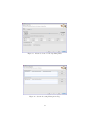
3.5
IP Cores View
ROCCC maintains its own database of compiled modules that can be viewed
at anytime. To view the contents of the database, click ROCCC → View →
IPCores on the Eclipse menu. The ROCCC IPCores view will open and display
all the inserted modules inside the database.
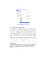
Figure 10: IP Cores View
You can view what ports are on a specific module in the database by selecting
a component in the IPCores view. The neighboring table will then display all the
port names, directions, port sizes, and types for that selected component. You
can delete a compiled component from the database by clicking the component
name in the IPCores View and pressing the Delete key. The component will
also be removed from the roccc-library.h file.
You can also use any of the components in the ROCCC database by having
a valid module or system open and selected, move the cursor to where you want
to insert a call to a module, and double click the desired component in the
IPCores view. This will add a function call to the double clicked component in
the open ROCCC file and will add #include roccc-library.h to the top of the
file. All that you will have to do after that is put which variables you wish to
pass into the desired component function call.
3.6
Creating a New ROCCC Project
To start using ROCCC with your own code from scratch, you first need to create
a new project. To create a new project, select ’ROCCC → New → Project as
shown in Figure 11.
Figure 11: Creating a New Project
28
A window will pop up asking for the name of the new project to make. Type
in the desired name of the project and press ”Ok.” Once that is done a new
project will show up in the project explorer with the name you chose. From
there, to add new modules or systems you either import them from already made
files or create new ones from scratch. To import premade modules or systems
into the project, use the Import → Module and Import → System under the
ROCCC menu. To create new modules or systems to be added to the project,
use the New → Module and New → System under the ROCCC menu.
3.7
Build to Hardware
Once a ROCCC module or system is ready to be compiled into VHDL code,
you want to use the Build command. To do this, open the desired module or
system inside the Eclipse editor and select the Build command in the ROCCC
menu or ROCCC toolbar. After that is selected, a window will open up asking
for which high-level compiler optimizations to use as in Figure 12.
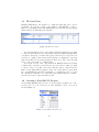
The build window consists of several pages which control different levels of
compiler optimizations. The user may select finish at any time and any pages
not modified will use the default values. The default values may also be set on
a page by page basis by selecting the ”Save Values As New Defaults” button.
Figure 12: High-Level Optimizations Page
On the first page you can select which high level compiler optimizations to
add to perform. Depending on whether you are compiling a module or a system,
you will see a different list of available optimizations to choose.
The second page available when compiling asks for which low-level compiler
optimizations to use as in Figure 13. These flags are same regardless of compiling
a module or system.
29
Figure 13: Low-Level Optimizations Page
The third optimization page available when compiling controls the extent
of pipelining in the generated hardware. As shown in Figure 14, the pipelining
may be controlled with a slider that adjusts the generated pipeline from fully
pipelined on the left to fully compacted on the right. When fully pipelined,
every operation will be placed into a separate pipeline stage, resulting in the
largest area but fastest clock. When fully compacted, the compiler will attempt
to put every operation into one pipeline stage, resulting in the slowest clock
speed but smaller area. When fully compacting code, instantiated modules will
retain their delay.
However, not all operations take the same amount of time to execute. To
naively have the compiler arbitrarily pack operations together without considering how expensive an operation is would give inconsistent results across different
components. Because of this, ROCCC allows you to specify weight values for
each basic operation in the advanced mode as shown in Figure 15. A larger
weight means that operation is more expensive in terms of execution time on
the desired platform. To edit these values, click the advanced tab at the top of
the Area vs Frequency page.
These weight values have no real absolute meaning, they only have meaning
relative to each other. For example, if our Mult operation takes twice as long
as our Add, we need to make sure we make the weight value for Mult is twice
that of Add. This can be done as (100 and 50) or (50 and 25), it doesnt really
matter as long as the weights are proportional to each other. In this case when
compaction occurs, the compiler would attempt to allow two chained additions
to happen together for every multiplication that is done.
If all the weights have the same value, that means that they all take the same
amount of execution time. Again, this can be achieved by having the weights
30
Figure 14: Basic Control of the Pipelining Phase
as all 1s or even all 500s, as long as they are all the same value. The default
weights that were distributed with ROCCC are the values we came up with for
targeting 150 MHZ on a LX-330. These weights combined with the pipeline
slider gives you precise control over how to tune your component in terms of
area and frequency.
Also available in the advanced view is control over the maximum allowable
fanout. When generating a circuit, if any register has a fanout larger than the
specified number registers are inserted along the paths in order to ease routing
constraints.
If compiling a system there is a fourth page in the compilation wizard for
managing the ways streams are accessed as shown in Figure 16. From here
you can select ”Add” to add managing info for either input or output streams.
From here a page will open asking for the stream name, the number of stream
channels, and for input streams, the maximum number of outstanding memory
requests at any time. Once pressing ”Finish” the values will be added to the
stream management page in the corresponding table you pressed ”Add” for.
Once these values are in the table, you can edit these values by double
clicking individual cells and changing the values. The number of outstanding
memory requests must be equal to or greater than the number of stream channels. Also, the number of stream channels must be a factor of the window the
data is being accessed from for that stream and the step size of the loop.
Once you have selected which optimizations to use and have set the arguments for the optimizations that require them, select Finish. This will run the
ROCCC toolchain on the selected open file inside the Eclipse editor. All output
from the compilation will be outputted on the console inside of Eclipse as shown
in Figure 17.
31
Figure 15: Advanced Control of the Pipelining Phase
Figure 16: Stream Accessing Management Page
32
Figure 17: Successful compilation
If the compilation finished successfully, you will see a VHDL folder in the
project directory next to the file you compiled that will have the generated
VHDL code for that system or module as shown in Figure 18
Figure 18: VHDL Subdirectory Created
The selected flags for each file are saved so that if you go to recompile a file
multiple times, it will load which flags were used during the previous compile.
The other way to compile a file is to right-click the desired file in the Project
Navigator and select Build to Hardware in the ROCCC submenu as shown in
Figure 7.
3.8
High Level Compiler Optimizations
In addition to standard compiler optimizations such as dead code elimination
and constant propagation, when compiling ROCCC code, the first page of the
build window will allow the user to select additional high level optimizations to
perform on the code. The choice of optimizations is different depending on if
the compiled code is a module or system. Note: When compiling a module, all
loops are fully unrolled automatically.
The available optimizations are:
33
3.8.1
System Specific Optimizations
• Systolic Array Generation: Transform a wavefront algorithm that
works over a 2-dimensional array into a one-dimensional hardware structure with feedback at every stage in order to increase the throughput while
reducing hardware.
Note: This optimization cannot be combined with other optimizations.
• Temporal Common Sub Expression Elimination: Detection and
removal of common code across loop iterations to reduce the size of the
generated hardware.
• LoopFusion: Merge successive loops with the same bounds and no dependencies.
• LoopInterchange: Switch the loop induction variables of two nested
loops.
• Loop Unrolling: Unroll the loop at the given C label by a specified
amount. If the loop has constant bounds, the loop can be fully unrolled.
Arguments:
Loop Label - The loop specified by the C label in the code.
Number of times to unroll - The number of times to unroll the loop. If
the loop has constant bounds, you can set the value to FULLY to fully
unroll the loop. If a system has all of its loops completely unrolled, it will
be transformed and compiled as a module.
• FullyUnroll: Fully unroll all loops in the original C code. If any of the
loops have variable bounds, this pass will stop compilation.
3.8.2
Optimizations for both Systems and Modules
• MultiplyByConstElimination: Replace all integer multiplications by
constants with equivalent shifts and additions.
• DivisionByConstElimination: Replace all integer divisions by constants with equivalent shifts and adds.
• Redundancy: Enable dual or triple redundancy for a module at a given
C label.
• InlineModule: Inline C code of specified modules as opposed to instantiating black boxes.
• InlineAllModules: Inline C code of all module instantiations, and if
those contain any other calls, continue inlining up to the specified depth.
34
3.9
Add IPCores
When working on a ROCCC project, you may want to integrate some hardware
modules that you have access to outside of ROCCC. Using this component would
require you to insert the already created component into the ROCCC database
so the compiler can incorporate it as well as using it in future compilations. To
do this, select Add → IPCore in the ROCCC menu. A window will pop up
asking for the details of the component as shown in Figure 19.
Figure 19: Add Component Wizard
First, specify the name and latency of the component. Next, you need to
add all of the ports for the added component. You need to specify at least one
input port and one output port before you can click Finish. If you need to edit
one of the already added ports, simply double click on the field you wish to
edit and you will be able to change the value of that field. Once everything is
added correctly, click Finish and the component will be added to the ROCCC
database. The component will now also be found in the IPCores view.
3.10
Create New Module
To start a new module from scratch, first make sure you have a valid ROCCC
project loaded or have created a new project as described in the Creating a new
Project section. Once you have a valid project open, select New → Module
under the ROCCC menu or toolbar to begin creating the new module. A new
window will open asking for the details of the new module as shown in Figure
20.
35
Figure 20: New Module Wizard
Input the name of the module and which project to add the new module to.
Next add all the ports that this module will have. If you ever need to edit an
already added port, simply double click the field you wish to edit and you will
be able to change the value of that field. Once everything is added correctly,
click Finish and the module will be added to the project. The new file will
open in the editor with the necessary starter code to begin coding the module
as shown in Figure 21.
Figure 21: Module Skeleton Code for MACC
3.11
Create New System
To start a new system from scratch, first make sure you have a valid ROCCC
project loaded or have created a new project as described in the Creating a
36
Figure 22: New System Wizard
new Project section. Once you have a valid project open, select New → System
under the ROCCC menu or toolbar to begin creating the new system. A new
window will open asking for the details of the new system.
Input the name of the system and which project to add the new system
to. Lastly, select how many stream dimensions the system will have. Once
everything is added correctly, click Finish and the system will be added to the
project. The new file will open in the editor with the necessary starter code to
begin coding the system as shown in Figure 23.
Figure 23: System Skeleton Code for WithinBounds
3.12
Import Module
If you are looking to add an already done ROCCC module C file to the current
project you are working on, you can use the Import Module command. To do
this, first have a valid project opened to import the module into. Next, click
Import → Module under the ROCCC menu. This will open up a window asking
for the file to import.
37
First, browse for the desired ROCCC module file to import. Secondly, type
the name of the module you are importing. Lastly, select which project to
import the module into. Once finished, click the Finish button at the bottom
and the selected module will be imported into the project and will show up in
the Project Navigator view. This does not add the module to the database, this
solely adds the module C code to the project.
3.13
Import System
If you are looking to add an already done ROCCC system C file to the current
project you are working on, you can use the Import System command. To do
this, first have a valid project opened to import the system into. Next, click
Import → System under the ROCCC menu. This will open up a window asking
for the file to import.
First, browse for the desired ROCCC system file to import. Secondly, type
the name of the system you are importing. Lastly, select which project to import
the system into. Once finished, click the Finish button at the bottom and the
selected system will be imported into the project and will show up in the Project
Navigator view. This does not create hardware code for the selected system,
this solely adds the system C code to the projects.
3.14
Intrinsics Manager
Certain operations in C require hardware blocks on FPGA. These include floating point operations and integer division. By selecting ’Manage → Intrinsics’
the user is able to select which IP cores to use. The intrinsics manager is shown
in Figure 24. By adding intrinsics the user is able to select which components
are inserted into generated datapaths by activating and deactivating individual
intrinsics.
3.15
Open ”roccc-library.h”
Every time a module is compiled, the interface struct and hardware function
prototype are added to the roccc-library.h file. If you ever need to view the
roccc-library.h file, simply select View → roccc-library.h under the ROCCC
menu. This will open up the roccc-library.h file in the default editor.
3.16
Reset Compiler
To reset the ROCCC database to its distribution state, simply click Settings →
Reset Database under the ROCCC menu. This will delete any added entries in
the ROCCC database and will clear all added modules under the roccc-library.h
file.
38
Figure 24: Intrinsics Manager
3.17
Testbench Generation
Once a module or system has been compiled with ROCCC and translated into
hardware, you can create a hardware testbench for simulation by selecting Generate → Testbench from the ROCCC menu. For modules, you can enter as
many test sets as you wish with their corresponding expected outputs. For systems, you will need to enter values for both the input scalars as well as all of
the input streams as shown in Figure 25. The stream files must consist of a list
of values separated by white space in the order in which they will be read.
3.18
Platform Generation
Once a module or system has been compiled with ROCCC, you can generate a
Xilinx PCore from it. You can do this by selecting ’Generate → PCore Interface
in the ROCCC menu as shown in Figure 26. ROCCC will then generate all the
necessary files and connections to make a PCore. If your component requires
any dependent files such as sub components or netlists, a window will pop up
asking for those files prior to generating the PCore files. The window will show
you all the required components it is looking for and ask for the necessary files
for each as in Figure 27.
You can either fill these sections out and let ROCCC handle all the moving
and packaging of the files or you can continue with the generation without specifying these and place them in the packaged folder later. Once the generation
of the PCore interface is complete, a folder named either ”PCore” will show up
next to the ROCCC file in the project explorer as in Figure 28
These folders should have all the files necessary to run the PCore on the
desired hardware as long as they support PCores on what you chose.
39
Figure 25: Testbench Generation
Figure 26: Generate a PCore
40
Figure 27: Dependent Files Window
Figure 28: Generated PCore Folders
PCores support being generated on all modules but currently not on systems.
3.19
Updating
There are a few ways to keep the ROCCC toolset up to date with the most
current version available. The first is by having the ROCCC GUI automatically
check for updates each time on startup. You can change whether or not you want
ROCCC checking for updates at startup in the preference page as in Figure 4.
The other way to check for updates is to manually check for updates by selecting
’Help → Check for Updates’ in the ROCCC menu as in Figure 29.
In both of these cases, ROCCC will check to see if there is a new version of
the compiler and if there is a new version of the GUI plugins. All messaging
about checking for updates will show up in the Eclipse console.
If there is an update for the compiler, it will ask if you would like to update.
Once selecting ”Yes” ROCCC will start patching the compiler to the latest ver-
41
Figure 29: Check For Updates
sion. If there is an update for the GUI plugins and you have selected you wanted
to update, ROCCC will download the latest plugins to the ”GUI” folder of the
distribution directory you installed. To complete installation of the plugins,
you must move the downloaded plugins from the ”GUI” folder of the ROCCC
distribution and place them inside the ”plugins” folder of the Eclipse directory.
It is also suggested you delete the old plugins from the Eclipse plugins folder as
well. Once this is done, restart Eclipse using the command ”./eclipse -clean”
in the terminal which should reload any new plugins and installation should be
complete.
42
4
C Code Construction
4.1
General Code Guidelines
ROCCC supports two styles of C programs, which we refer to as modules and
systems. Modules represent concrete hardware implementations of purely computational functions. Modules can be constructed using instantiations of other
modules in order to create larger components that describe a specific architecture.
System code performs repeated computation on streams of data. System
code consists of loops that iterate over arrays. System code may or may not
instantiate modules. System code represents the topmost perspective and generates hardware that interfaces to memory systems.
4.1.1
Limitations
ROCCC is not designed to compile entire applications into hardware and has
certain general restrictions on both module and system code. ROCCC is continually in development, so these restrictions may fluctuate or be eliminated
entirely in future releases. ROCCC 2.0 currently does not support:
• Logical operators that perform short circuit evaluation. The ”&” and ”|”
operators do work and should be used in place of ”&&” and ”||”
• Generic pointers
• Non-component functions, including C-library calls
• Shifting by a variable amount
• Non-for loops
• Variables named ’C’
• The ternary operator (?:)
• Initialization during declaration
• Array accesses other than those based on a constant offset from loop induction variables
4.2
Module Code
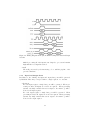
Module code represents a hardware building block to be used in larger applications. Modules are computational datapaths and are written as computational
functions. All inputs to modules are passed in by value and all outputs are
passed by reference. Inputs must only be read from and output ports can only
be written to inside the function. We do not support writing to an output
port multiple times inside the function. Modules can only process scalar values
43
// Example module code
// Input parameters must
// come before output
// parameters
void FIR(int A0, int A1,
int A2, int A3,
int A4,
int& result)
{
const int T[5] =
{3,5,7,9,11} ;
result = A0 * T[0] +
A1 * T[1] +
A2 * T[2] +
A3 * T[3] +
A4 * T[4] ;
}
(a)
(b)
Figure 30: (a) Module Code in C and (b) generated hardware
and cannot have arrays as input or output variables. Internal variables may be
created but are not visible outside of the module.
Figure 30a shows a simple FIR filter written as a module. This code takes five
inputs and computes a single output. When compiled, the hardware generated
will resemble the circuit shown in Figure 30b. The interface to the module is
exactly as described by the parameter list, the integer array T is not visible
outside of the module.
Modules do not generate addresses or fetch values from memory, but instead
have data pushed onto them, and then output scalar values after all computation
has been performed. They are completely pipelined and can support processing
new data every clock cycle.
If a module contains a loop, it will automatically be fully unrolled. Hence,
any loop inside of a module must have an end bound that can be statically
determined. Figure 31a provides an example of the supported loop structure
inside modules.
After unrolling, constant and copy propagation, we end up with the hardware
as shown in Figure 31b which is a single multiply as we would expect. There is
no loop control or other control created as the loop has been removed.
4.3
System Code
System code performs computation on streams of data and produces streams of
data. Scalars may also be read as input and generated as output, but as opposed
44
// This module contains a loop, it will
// automatically be fully unrolled
void Squared(int x, int& y)
{
int total ;
int i ;
total = 1 ;
for (i = 0 ; i < 2 ; ++i)
{
total *= x ;
}
y = total ;
}
(a)
(b)
Figure 31: (a) Using a loop in module code and (b) resulting hardware
to modules, input scalars are read once at the beginning of computation and
output scalars are only generated once at the end of computation.
Similar to module code, system code is written as a void function that takes
input and output parameters. Input scalars are passed by value, output scalars
are passed by reference, and both input and output streams are passed as pointers. The function definition must declare inputs before outputs. Although
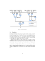
passed as pointers, the internal use of streams must be through array accesses.
An example of system code is shown in Figure 32a. This code takes a single
input scalar that is used to determine the length of the incoming streams, two
input streams V1 and V2, and an output stream Sum. The computation adds
all elements of the two input vectors and outputs them to the Sum stream.
Like module code, all inputs must be declared in the parameter list before any
outputs.
The generated hardware is shown in Figure 32b. Each stream specified in the
C code generates a memory interface that includes an address generator (AG)
and a BRAM FIFO structure. The specifics of the hardware communication
protocols are discussed in Section 5. Data reuse is handled through the creation
of smart buffers, which is detailed in Section 4.8.7. The code located in the
innermost loop will be translated into a datapath that is separate from the
control.
4.3.1
Windows and Generated Addresses
When generating code, we infer the size of the memory we are accessing from
both the loop bounds and the size of the accessed window. For example, the
loop bounds in Figure 33 suggest a 10x10 memory. However, the code inside the
loop accesses a 3x3 window, so we generate code that assumes a 13x13 memory.
45
// Example system code
// Streams are passed as
// pointers but treated
// as arrays
void VectorAdd(int N,
int* V1,
int* V2,
int* Sum)
{
int i ;
for (i = 0 ; i < N ; ++i)
{
Sum[i] = V1[i] + V2[i] ;
}
}
(a)
(b)
Figure 32: (a) System Code in C and (b) generated hardware
46
void WindowSystem(int* A, int* B)
{
int i, j ;
for (i = 0 ; i < 10 ; ++i)
{
for (j = 0 ; j < 10 ; ++j)
{
B[i][j] = A[i][j] + A[i+2][j+2] ;
}
}
}
Figure 33: Accessing a 3x3 Window
The addresses we generate will be the same as in C, and note that if run in C
on a 10x10 array the results will be undefined.
When fetching the first window, we will therefore generate the offsets 0, 13,
and 26 for the first column and NOT 0, 10, 20. Similarly, we will generate the
offsets 1, 14, and 27 for the second column, and 2, 15, and 28 for the third
column of the window.
Additionally, we perform a normalization step on the window accesses to
adjust for negative offsets. If the C code accesses an array with a negative
offset, for example A[i-2] and A[i-1], we normalize these values to start at location 0, meaning the previous offsets will be adjusted to A[i] and A[i+1]. After
the normalization, we determine the size of the memory rows we are accessing
identically as above.
4.3.2
N-dimensional arrays
ROCCC can accept arbitrary dimension arrays. Figure 34 shows example C code
that both inputs a three dimensional array and outputs a three dimensional
array. When declaring an N-dimensional array, the parameter must be a Ndimensional pointer.
4.3.3
Feedback detection
Variables whose values are used in multiple iterations of the for loop in system
code are detected and turned into feedback variables. Figure 35 shows example
code that contains a feedback variable. In this code, the value of currentMax is
used in the initial loop iteration and is then carried through all of the additional
loop iterations.
When converting the code in Figure 35a into hardware, we get a circuit that
resembles that in Figure 35b. All variables that are determined to be feedback
variables will have an additional hardware input port generated for the initial
value of the variable. Subsequent iterations of the datapath can only be executed
once the value of the feedback variable is known, which in the worst case will be
at the bottom of the pipeline. This feedback may potentially decrease circuit
47
// Example N-Dimensional code
void NDimensional(int*** A, int*** B)
{
int i, j, k ;
for (i = 0 ; i < 10 ; ++i)
{
for (j = 0 ; j < 10 ; ++j)
{
for (k = 0 ; k < 10 ; ++k)
{
B[i][j][k] = A[i][j][k] ;
}
}
}
}
Figure 34: A system with a three dimensional input and output stream
throughput if the C code requires the feedback variable to be determined at the
bottom of the pipeline and used at the top of the pipeline.
Feedback variables are not output at the end of computation and if you wish
to have the final value output you must assign a separate output variable, as
shown in Figure 35b.
4.3.4
Summation reduction
A special condition of feedback variables is a summation reduction. When the
feedback detected is purely performing a summation reduction the feedback can
be performed in one clock cycle and does not necessarily affect the throughput
of the circuit.
An example of the code recognized as a summation reduction is shown in
Figure 36a. The hardware generated, as shown in Figure 36b, will contain a
datapath that handles the feedback internally and can support full throughput
on the data streams.
4.4
Instantiating Modules
Both module code and system code can instantiate other modules to be integrated directly into the generated hardware. When a module is compiled, it
is exported for use in other code. All modules have header information placed
into the file ”roccc-library.h.” These functions can be called from other ROCCC
code and each function call will be translated into a module instantiation.
The system code shown in Figure 37a processes a data stream and instantiates the module that was shown in Figure 30. When compiled, the generated
hardware will resemble the circuit shown in Figure 37b.
IMPORTANT NOTE: Currently, array references can be used as inputs to
modules but the outputs of modules can not be mapped to array references.
48
// Example code with feedback
void MaxSystem(int N, int* A,
int& final)
{
int i ;
int currentMax ;
for (i = 0 ; i < N ; ++i)
{
if (A[i] > currentMax)
{
currentMax = A[i] ;
}
else
{
currentMax = currentMax ;
}
final = currentMax ;
}
}
(a)
(b)
Figure 35: (a) System Code That Contains Feedback and (b) Generated Hardware
A
// Example summation code
void Summation(int* A, int* B,
int& final)
{
int i ;
int output ;
for (i = 0 ; i < 100 ; ++i)
{
output = A[i] ;
output += A[i] ;
final = output ;
}
}
Smart Buffer
Datapath
output
final
(a)
(b)
Figure 36: System Code That Results in a Summation Reduction
49
If you wish to accomplish this, you must declare an intermediate temporary
variable and assign the output of the module to this variable and then assign
the variable to the output array. This is shown in Figure 37a as the output
of FIR must be mapped to the variable tmp and then assigned to the output
stream B.
4.4.1
Inlining Modules
The user has control of if module instantiations are treated as black boxes or
inlined. When inlined, the individual operations of the module are exposed to
the top level design and can be optimized around at the expense of increased
compile time. As an example, Figure 37c shows the resulting circuit structure of
the FIR system code shown in Figure 37a. Note that instead of a black box the
top level design has all of the individual operations exposed and may perform
additional optimizations on this code.
4.5
Control Flow
ROCCC code supports arbitrary if statements through predication. The quality
of the generated circuit is directly affected by the use of predication, so care
should be taken in constructing the C code to minimize logic.
In the simplest case, an if statement that determines one of two values to
store into a variable will be translated into a boolean select statement. Figure
38 shows the transformation undergone from original C code to intermediate
representation and finally to the generated hardware. If statements written in
exactly this way will always result in a mux in the generated hardware.
All other combinations of if statements will be reduced to this form through
predication. If there are any paths through which a variable might not be
initialized, the generated hardware will either choose a default value of 0 create
a feedback variable that requires an initial value. An example of this is shown
in Figure 39. The variable x is only assigned if the expression (value > 5) is
true. In the generated hardware we must assign a value to x regardless of the
expression’s result, and so we assign a default value. In modules, this default
value is 0, while in systems the default value is itself, which will introduce a
feedback variable in a way that the user might not have expected.
4.6
Legacy Code
In previous versions of ROCCC, modules and systems were coded slightly differently. We still support compilation of legacy code, although newer features
such as inlining are not supported for legacy code and mixing legacy code with
new style code may cause problems in the future as legacy code is deprecated.
4.6.1
Legacy Module Code
Legacy module code must define both an interface and implementation. The
interface is described as a struct that identifies all of the inputs and outputs
50
void FIRSystem(int* A, int* B)
{
int i ;
int tmp ;
for (i = 0 ; i < 10; ++i)
{
// Module instantiation
FIR(A[i], A[i+1], A[i+2],
A[i+3], A[i+4], tmp) ;
B[i] = tmp ;
}
}
(a) C Code
(b) Generated Hardware
(c) After Inlining
Figure 37: (a) Code That Instantiates a Module, (b) the Generated Hardware,
and (c) Generated Hardware After Inlining
51
if (value > 5)
{
x = 1 ;
}
else
{
x = 2 ;
}
x = ROCCCBoolSelect(1, 2, (value > 5)) ;
(a)
(b)
(c)
Figure 38: Boolean Select Control Flow. (a) In the original C, (b) in the
intermediate representation, and (c) in the generated hardware datapath.
if (value > 5)
{
x = 1 ;
}
pred = (value > 5) ;
x = ROCCCBoolSelect(1, x, pred) ;
(a)
(b)
(c)
Figure 39: Predicated Control Flow (A) in the original C, (B) in the intermediate
representation, and (C) in the generated hardware.
52
typedef struct
{
int A0_in ;
int A1_in ;
int A2_in ;
int A3_in ;
int A4_in ;
int result_out ;
} FIR_t ;
FIR_t FIR(FIR_t t)
{
const int T[5] = { 3, 5, 7, 9, 11 } ;
t.result_out = t.A0_in * T[0] + t.A1_in * T[1] +
t.A2_in * T[2] + t.A3_in * T[3] + t.A4_in * T[4] ;
return t ;
}
Figure 40: Legacy Module Code
to the module. Input ports must be identified by adding the suffix ” in” and
output ports must be identified by adding the suffix ” out.”
The implementation function must be a function that returns and receives
an instance of this struct by value. Any return statements that are not at the
end of the function are ignored and cannot be used as a form of control flow.
All computation inside this function will be translated to hardware.
The FIR filter shown in Figure 40 is written in this style. Note that the
hardware generated for this code is nearly identical to the hardware generated
for the same code written in Figure 30. The only difference will be in the
ordering of the ports once compiled.
IMPORTANT NOTE: When compiling Legacy ROCCC modules, the order
in which you pass the parameters is not necessarily the order in which you
declared them in the struct. The order in which you pass parameters must
match the order in which they appear in the struct as exported in the ”roccclibrary.h” file. If using the GUI, this ordering is available by double-clicking the
module in the IPCores view. Modules written in the new style will have the
parameters in the same order as written.
4.6.2
Legacy System Code
Legacy system code is nearly identical to the new style system code with the
exception that parameters were not accepted. Input and output arrays and
scalars are declared locally and inferred during compilation.
53
4.7
Compiling
Compiling should be handled through the GUI.
In order to compile without using the GUI, you must call the program ”createScript,” located in the Install/roccc compiler/src/tools directory. This program takes two arguments, the C file and a file listing optimizations to perform.
A script file ”compile suif2hicirrf.sh” is then generated. Run this script and
then the script ”compile llvmtovhdl.sh” on the hi cirrf file to generate VHDL.
Details on this process are available in the Developer’s Manual.
4.8
Hardware Specific Optimizations
There are several features specific to ROCCC that allow you to create specific hardware and are not reflected in the software. These include bit-width
specification, systolic array generation, and temporal common subexpression
elimination.
4.8.1
Specifying Bit Width
Every integer variable you declare in the C code can have a nonstandard bit
width tailored to your application. The supported floating point bit widths are
16, 32, and 64, with the default being 32 bits. The choice of cores instantiated in
the datapath will be based upon the bit width of the variables passed to them.
Smaller bit width variables will be extended to take advantage of the larger
cores unless no such core exists, in which case the variables will be truncated to
use the largest core available.
The quality and precision of the generated VHDL can vary based upon how
the C is specified, so use caution. By default, all operations are expanded to
the highest precision before being performed and then truncated if necessary as
the last step. In the generated VHDL, an N bit addition is stored into an (N
+ 1) bit value and a multiplication between two N-bit numbers is stored into a
number with 2N bits. The user may select the optimization ”MaintainPrecision”
to truncate at every step.
Specifying the specific bit width is done by declaring a typedef at the beginning of your program. This typedef must be in the form of ROCCC intX where
X is any positive number, as shown in Figure 41. This type can then be used
to declare any variable with the appropriate size.
4.8.2
Systolic Array Generation
Systolic array generation is an optimization that takes a wavefront algorithm
operating on a two-dimensional array and converts it into hardware consisting
of a single dimensional array of elements that feed back to each other. The
original C code must be in the form of a doubly nested for loop that calculates
the value of a two-dimensional array based upon some function of the previous
elements of that array.
54
typedef int ROCCC_int12 ;
void Test(ROCCC_int12 a_in, ROCCC_in12& b_in)
{
// ...
}
Figure 41: Declaring And Using A Twelve Bit Integer Type
L1: for (i = 0 ; i < 100 ; ++i)
{
for (j = 0 ; j < 100 ; ++j)
{
A[i][j] = A[i-1][j-1] + A[i][j-1] + A[i-1][j] ;
}
}
Figure 42: C Code To Generate A Systolic Array
In order for systolic array generation to recognize the optimization, the outer
loop must be labelled as shown in Figure 42.
The current version of systolic array generation only transforms a precise
software architecture into a specific instance of a systolic array. The code must
have a single two-dimensional array where the value of every cell is based upon
some function of the cells located to the north, west, and northwest. Optionally, the C code may have a constant array of values based upon the outer loop
bounds and a single dimensional input array based upon the loop bounds of
the innermost loop as seen in the Smith Waterman example. Any other software architecture is not currently supported for the systolic array generation
optimization.
After transformation, the resulting hardware will expect a one dimensional
input array (A input) and produces a one dimensional output array (A output)
in place of the original two-dimensional array. The input stream A input should
be the values of the topmost row of the original two-dimensional array. The
output stream A output will generate the bottom row of the original twodimensional array. All of the intermediate values are discarded and not output in the generated hardware structure. Additionally, the first column of the
original two-dimensional array must be passed in as scalars to the resulting
hardware.
4.8.3
Temporal Common Subexpression Elimination
Temporal common subexpression elimination (TCSE) analyzes loops and detects common code across loop iterations. For example, if the same value is
calculated in loop iteration 1 and loop iteration 2, this will be detected. When
55
Figure 43: Block Diagram Of Max Filter System
Figure 44: Block Diagram Of Max Filter System After TCSE
generating hardware, we take advantage of this fact and create feedback variables that eliminate redundant computations.
TCSE can only be performed on system code. The code does not have to
be written in any special way to take advantage of TCSE.
An example of the difference in hardware generated can be see in Figures
43 and 44. These block diagrams show the original structure of the Max Filter
System hardware that contains four Max Filter modules and operates on a
sliding 3x3 window and the Max Filter System after TCSE has been performed.
After TCSE, the generated hardware only has two Max Filter modules and two
have been replaced with feedback variables.
The generated hardware does require initial values for each piece of hardware
eliminated, so you might have to change the way you pass data into the hardware
depending on if you perform TCSE or not.
4.8.4
Arithmetic Balancing
The user has the choice of performing arithmetic balancing on the generated
hardware. The optimization finds expressions composed of a single operator
performed in serial, and changes the order that the subexpressions are calculated in to minimize the time to calculate the expression. Only associative and
commutative operators are balanced; currently, addition, multiplication, and
56
bitwise AND, OR, and XOR are balanced. For example, the statement ”a =
b + c + d + e” in software will be calculated serially. By performing arithmetic balancing, the statement is changed into ”a = (b + c) + (d + e)”, with
”b+c” and ”d+e” calculated in parallel. Because floating point operators are
not strictly associative and commutative, and order of execution matters when
dealing with overflow, this optimization may change the final result when using
floating point values.
4.8.5
Copy Reduction
ROCCC automatically inserts copy registers in between pipeline stages if a value
is not used immediately after it is calculated. If an operation could correctly be
calculated in several different pipeline stages, one of those stages will minimize
the total bits that are copied (both coming into that operation from previous
stages, and leaving that operation to later stages that use the calculated value).
This pass attempts to find a placement for operations that minimizes the total
number of copied bits. Starting with the edge in the use-def graph that has the
most number of bits copied, edges are ”tightened” by moving the nodes at the
edges ends toward each other. By repeating this process, and saving a snapshot
of the graph whenever a minimal number of copied bits is found, eventually a
local minimum is found that minimizes the number of copied bits. This can take
as long as O(E), where E is the number of edges in the use-def graph, although
in practice a minimum is found quickly.
4.8.6
Fanout Tree Generation
When compiling high level code, the amount of parallelism that is generated in
hardware may not be readily apparent. High fanout can seriously affect the clock
rate or area of the generated circuit, and so we have added user control to specify
the maximum allowable fanout for any register in the generated circuit. If the
fanout exceeds this number, ROCCC generates a tree of registers in separate
pipeline stages, increasing the latency but shortening the clock and simplifying
the routing.
4.8.7
Smart Buffers
When generating code for systems, array accesses are analyzed looking for possible reuse between loop iterations. These reuse patterns can be exploited and
reduce the number of off-chip memory accesses. The generated hardware will
contain Smart Buffers to exploit the reuse between loop iterations, which internally consist of registers that cache the portion of memory reused.
The code in Figure 45 requires a 3x3 window from the memory A in order to
execute each loop iteration. Note that as in the C code, the ROCCC generated
hardware will access rows 0-6 and columns 0-6 of the image even thought the
loop bounds are < 5. As shown in Figure 46, code that accesses a sliding
3x3 window over a larger memory can reuse six values between loop iterations
57
for(i = 0 ; i < 5 ; ++i )
{
for (j = 0 ; j < 5; ++j)
{
row1 = A[i][j] + A[i][j+1] + A[i][j+2] ;
row2 = A[i+1][j] + A[i+1][j+1] + A[i+1][j+2] ;
row2 = A[i+2][j] + A[i+2][j+1] + A[i+2][j+2] ;
B[i][j] = row1 + row2 + row3 ;
}
}
Figure 45: System Code That Accesses a 3x3 Window
Figure 46: 3x3 Smart Buffer Sliding Along a 5x5 Memory
(shown with X’s in the diagram). The smart buffer initially reads nine values
from memory and exports all nine to the datapath for the first loop iteration,
and for subsequent iterations only three are read for each loop iteration.
The code as shown in Figure 47 will be analyzed by ROCCC and determined
that no reuse occurs between loop iterations. In this case, a FIFO interface is
generated. For each loop iteration, two elements are read in, as in Figure 48.
No reuse can be exploited between consecutive loop iterations.
for (i = 0 ; i < 5; i += 2)
{
B[i] = A[i] + A[i+1] ;
}
Figure 47: System Code That Reads From A Fifo
58
Figure 48: Memory Fetches When Using A FIFO
59
5
Interfacing With Generated Hardware
5.1
Port Descriptions
The VHDL generated by ROCCC communicates with the external platform in
a variety of ways described in this section. All inputs and outputs that connect
to ROCCC code are assumed to be active-high.
5.1.1
Default Ports
Each hardware module and system generated by ROCCC will contain six ports
by default. These default ports are clk, rst, inputReady, outputReady, done,
and stall. Their use is described here:
• clk
The clk port is the clock of the hardware and should be connected to a
clock signal. All processes internal to ROCCC code trigger off of the rising
edge of the clock. All ROCCC components and systems assume a single
clock to drive all the hardware.
• rst
The rst port is the reset signal to the generated hardware. Driving the
reset port high resets the hardware to an initialized state. As long as
the reset port is held high, the hardware will remain in the reset state,
regardless of the inputs. After bringing the reset port low, the hardware
will begin responding to the input signals. The hardware generated by
ROCCC requires the reset port to be driven high for at least one clock
cycle for initialization purposes. Not doing so may leave the component
in an uninitialized state. The use of the reset signal and the initialization
of hardware that contains both input registers and input streams is shown
in Figure 49.
• inputReady
The inputReady signal should be driven high when the signals that correspond to input scalars are valid. As long as the inputReady signal is
high, input scalars will be read on every rising edge of the clock. Setting
the input scalars to valid data and setting inputReady high should be
the first thing done by any interfacing code. Even if no input scalars are
used, streams will wait to generate addresses and request data until after
inputReady is driven high.
• outputReady
The outputReady port goes high when valid data is placed on the output
scalar ports of the hardware. The output data is valid simultaneously with
the outputReady signal being high.
• done
The done port goes high when the hardware generated by ROCCC has
60
Figure 49: Timing Diagram Of A System With Both Input Scalars And Input
Streams
finished processing all of the input it was designed to process and remains
high until the reset signal is asserted.
• stall
The stall port is used by the interfacing code to stall the pipeline of the
generated hardware.
5.1.2
Input And Output Ports
In addition to the default ports, input and output data ports will be generated
by ROCCC. These may correspond either to single registers or to streams.
• Registers
For each input register, a single data port will be generated. When generating modules, all inputs are treated as registers. When generating
systems, any single variable that acts as input to the main loop will be
treated as an input register.
For each output register, a single data port will be generated. When
generating modules, all outputs are treated as registers. When generating
systems, any single variable that acts as output to the main loop will be
treated as an output register.
61
*+, -)# )#2++ "./0#1(2%3
45".
89
!"#$"%#&'()#
!5".
:
6570#
8@
70#/0#1(2%3
%7.(
Figure 50: Block Diagram
Of A Generated Module
;<=>?
Figure 50 provides a block diagram of a ROCCC generated module. This
module includes both the default ports (located on the top and bottom)
but also the user defined ports, which may be variable bit size (located on
the left and right).
• Streams
For input streams, several ports will be generated: a write clock port, a
write enable port, a full port, an address ready port, a positive number of
input ports, and the same number of address ports. The number of input
ports and address ports will be equal to the number of channels the user
specifies for the stream, and needs to be a factor of both the window size
and the step window size.
Figure 51 shows the block diagram of a generated system that communicates with a multi-dimensional buffer. The default ports are still generated
(located on the top and bottom of the figure) as well as the interface to
the streams. In addition to the ports generated for streams, input and
output registers can be created as well.
For output streams, several ports will be generated: a read clock port, a
read enable port, an empty port, a poitive number of output data ports,
and the same number of address ports. For example, the code shown in
Figure 52 will result in hardware similar to that shown in Figure 53 with
each write to the output stream being serialized onto the same data port.
Similar to the input ports, the number of output data ports and address
ports will be equal to the number of channels the user specifies for the
stream and needs to be a factor of both the window size and the step
window size.
62
*+, -&' &'2++ ./01'#(23%
456*+,
45./
456-.'((/
45:1++
45233-(&&5-3%
45233-(&&
89
89
!"#$%&'()
=5()0'%
=5-(23(/
89
89
71'01'#(23%
=5-*+,
=5*>2//(+?
=5233-(&&
37/(
!";<9
Figure 51: Block Diagram
Of A Generated System
for(i = 0 ; i < 5; ++i)
{
B[i] = A[i] + A[i+1] ;
B[i+1] = A[i+1] + A[i+2] ;
B[i+2] = A[i+2] + A[i+3] ;
}
Figure 52: C Code That Writes To Three Locations In The Same Stream Each
Loop Iteration
63
.%/01.2"00)(,,
:;
4(%<4' :;
.%0'4 :;
17'87'9("0+
01/(
$ABC:
3&F ),' ,'"&& %/87'9("0+
E2.3&F
:;
E234"//(&@
E2.)%'((/
E257&&
E2"00)(,,2)0+
E2"00)(,,
:;
67'87'*')("-=
>#"-8&(
:;
17'87'9("0+
:;
?2)3&F
?234"//(&@
?2(-8'+
?2)("0(/
?2"00)(,,
01/(
$ABCD
Figure 53: Block Diagram Of Generated
Hardware For Code That Writes To
Three Locations Each Loop Iteration
Figure 54: Timing Diagram Of Module Use
5.2
5.2.1
Interfacing Protocols
Input Registers
Input registers are used by both module and system code. They need to be
set when inputReady is driven and are sampled on the rising edge of the clock.
Driving the input registers is the responsibility of the calling code. In modules,
the input registers can be changed every clock cycle. In systems, the input
registers may be set only once, and must be set before passing any data to the
input streams. See Figure 49 for the timing of interfacing with system code’s
input registers and Figure 54 for the timing of driving a module’s input registers.
5.2.2
Input Streams
The input stream address generation and the input protocol are decoupled,
allowing address generation to happen independent of incoming data. In particular, there are two ports dealing with address generation and four that deal
64
5&--'*67(&0&70.7&780+,&9
:;'0<7-'*6#,7&((+,--76,*,+&0'.*=
!"#$
%&#'()'*
(&0&)'*
(&0&2
(&0&3
B/##)./0
&((+,--)+(1)./0
&((+,--)./0
&((+2
&((+3
&((+4
>?@7ACode Reading From A Stream With
Figure 55: Timing Diagram Of Generated
Memory Addresses
with input data.
When an address is being generated, the address rdy port will be brought
high and the address port will hold the address of the value needed. The address rdy will only be held high for one clock cycle for each individual address
being generated. If addresses are being generated in consecutive clock cycles,
the address rdy port will be continuously high.
The user defined interfacing code needs to service memory requests in a
FIFO fashion. ROCCC generated code expects the data we receive to be in the
exact order as requested. When data is ready, if the full port is not currently
high, the data must be placed on the input data port(s) and write enable must
be asserted and held high for a clock cycle. As long as full remains low, write
enable can be kept high and data can be put onto the data port(s) every clock
cycle.
In order to allow the fastest possible streaming, all data is read synchronously,
but the pop/valid handshake is asynchronous. The pop and valid signals can be
treated as synchronous statements, although this limits the data transfer rate
to the ROCCC generated code with a data transfer occurring every other clock
cycle, with alternating cycles devoted to the handshake protocol. An example
of this timing protocol is shown in Figure 55.
The number of outstanding memory requests generated by the ROCCCgenerated code is independent of the reading of data and is user configurable.
As an example, shown in Figure 56, when the number of outstanding memory
requests is set to two we can generate a total of 2 memory addresses before we
stop. Data can be read at any time during memory generation although we
assume that all data being received happens in the order in which we requested
it.
If the user has specified that a given stream is a multi-channel stream, then
it is necessary to set all channels of the input with valid data before asserting
the valid signal. The channels in the ROCCC generated code are numbered
from 0 to N and it is up to the user generated interfacing code to place the
oldest data in channel 0, the second oldest data in channel 1, and so on. Once
65
4&--'*56(&0&60.6&670+,&8
95,*,+&0'*5636&((+,--,-:
!"#$
%&#'()'*
(&0&2
(&0&)'*
(&0&3
&((+,--)+(1)./0
&((+,--)./0
&((+2
&((+3
&((+;
&((+<
5,..'*67-,(,7(17,78(&),9
Figure 56: Timing Diagram Of Generated
Code Reading From A Stream With
:6)*)&,('*67;7,--&)..).<7;7'*=2(7"/,**)#.>
Multiple Outstanding Memory Requests
!"#$
%&'())*+'*
-,(,+"/,**)#0+'*
-,(,4
-,(,+"/,**)#0+'*
-,(,;
?2##+12(
,--&)..+&-3+12(
,--&)..+"/,**)#0+12(
,--&4
,--&@
,--&)..+"/,**)#0+12(
,--&;
,--&A
Figure 57: Timing Diagram Of Generated Code Reading From A Stream With
Multiple Channels
all channel data has been fetched, the interfacing code should set valid high and
hold it high until pop is seen to be high. An example of this timing protocol is
shown in Figure 57.
5.2.3
Output Scalars
Output scalars are driven when outputReady is driven. The number of clock
cycles before outputReady goes high after driving inputReady is based off the
delay of the pipeline. Code that interfaces with systems should ignore outputReady; if values are to be sampled every iteration of the loop, then a stream
should be used. System code that properly uses output scalars should only
interested in a final value, which will be valid when done goes high, not when
outputReady goes high.
66
2)'3".#45,(',(46(7%.&48%9.:3+7
!"#$
%&'()*+,(
-.(.*+,(
-.(./
-.(.0
-.(.1
.--7%<<*+,(
.--7/
.--70
.--71
7%.-%;*3;
Figure 58: Timing Diagram of Output Streams
5.2.4
Output Streams
Output streams have some number of data ports, the same number of address
ports, and three ports necessary for a fifo-style interface. The fifo interface
protocol of the output streams is similar to the fifo interface protocol of the
input stream. When the output controller has valid data from the datapath,
the first element of the stream is written to the data port(s), and the address
of that data element is written to the corresponding address port. The empty
port is brought low, signaling there is data in the fifo. When the read enable
signal is brought high, the first data element is put onto the data port(s) and
the address port is loaded with that element’s address. See Figure 58 for an
example of the timing protocol for output streams.
Because the outputController is serializing data calculated in parallel, the
datapath must be stalled until all of the data is serialized. This happens entirely internally, but functions equivalently to bringing the stall port high - the
datapath is stalled, the inputController continues to read but will not push data
onto the datapath, and other output streams may run out of valid data. For
this reason, it is important not to rely on a specific timing for any stream interfacing. Rather, the fifo interface should be relied on to guarantee that data
is transfered correctly.
If it is imperitive that data not be serialized, it is preferred to create several
output streams or to create a multi-channel stream over using output scalars as
psuedo-streams.
5.2.5
Done
The done signal works differently, depending on if it is coming from module or
system code. Module code will drive the done signal high as soon as the first
value is processed; this can safely be ignored by any code interfacing with a
ROCCC module, as modules are stateless and can never be considered done.
System code will drive the done signal high on the rising edge of the clock after
the last output values are set. Figure 59 provides an example of the done signal’s
67
Figure 59: Timing Diagram Of The End Of A System’s Processing
behavior in a typical system.
5.2.6
Stall
The stall signal allows the interfacing code to stall the datapath in both modules
and systems. Stalls are not instantaneous - it takes 1-2 clock cycles for the stall
signal to propogate all the way up the datapath, to both the input and output
controller. In hardware, a common use for a stall signal is when interfacing with
memory that may become full. However, both input and output streams are
two-way handshakes, and any stream can be ”stalled” by simply not completing
the handshake. For this reason, and because stalls are not instantaneous, stalls
should be reserved for the case when there is no alternative.
When the stall signal is brought high, both input and output streams will
continue to interact with any interfacing code. However, the datapath will be
frozen, and data will not be pushed onto the datapath. Again, prefer to handle
full memory in the stream interface, and not with the stall signal.
5.3
5.3.1
Memory Organization
Input Streams
Input streams will generate an address for each requested value. Both one
dimensional and two dimensional streams generate addresses for each requested
value and it is up to the interfacing code to decide how to treat these values.
The addresses that are generated by the system when accessing memory are
assuming an input memory of a certain size. This assumed size is based off of
several factors, including both the window size of the input and the size of the for
loops driving the window. For example, given the C code for MaxFilterSystem as
shown in Figure 60, the window size is 3x3 andthe for loop size is width x height.
Given these values the input memory size is (width + 3 − 1) ∗ (height + 3 − 1). To
traverse a memory of size 20x20, the width and height passed in to the hardware
need to both be 18 (20 + 1 − 3).
When processing the code in Figure 60, both height and width will become
input registers and need to be set along with inputReady. Only then is it safe to
68
for(i = 0 ; i < height ; ++i)
{
for (j = 0 ; j < width ; ++j)
{
MAX(window[i][j], window[i][j+1], window[i][j+2], maxCol1) ;
MAX(window[i+1][j], window[i+1][j+1], window[i+1][j+2], maxCol2) ;
MAX(window[i+2][j], window[i+2][j+1], window[i+2][j+2], maxCol3) ;
// Find the maximium of the three columns
MAX(maxCol1, maxCol2, maxCol3, finalOutput) ;
}
}
Figure 60: C Code For MaxFilterSystem Which Uses A 3x3 Window
begin returning valid data to the component’s request for window elements; not
setting height and width to the correct values will result in the wrong addresses
being generated.
5.3.2
Output Streams
The memory layout for output streams follows the same rules as the memory
layout of input streams. The window size and the for loop end values will both
be used to calculate the address of each value’s location in memory. For the code
in Figure 52, the first iteration through the loop will calculate B[i], B[i + 1],
and B[i + 2] with i = 0, and so the outputted address for B[i], B[i + 1], and
B[i + 2] will be 0, 1, and 2, respectively. On the second iteration through the
loop, i = 1, so the outputted address for B[i], B[i + 1], and B[i + 2] will be 1,
2, and 3, respectively. Multi-dimensional code works similarly.
One note to make is that there are no guarantees make about the order of
data comping out, nor are there any guarantees about the number of times a
value may be output; in the previous example, it is easy to see that element B[1]
was written in both the first and second iteration of the loop. Elements written
multiple times in different loop iterations may be actually written to more than
once, or values may be cached to eliminate redundant writes to memory. In any
case, it is important not to rely on a particular behavior.
5.3.3
Systolic Arrays
After using the systolic array optimization, two input streams and a set of
input registers are created as inputs. The input registers should be loaded with
the first column of the matrix, and the top row of the matrix is fed in as a
stream. The input array T is also fed in as a stream. Refer to Figure 64 for
the relationships between the original two dimensional array and the created
registers and input streams.
69
Figure 61: Basic Dataflow
5.4
Pipelining
Pipelining in ROCCC is guided by user-provided weights of basic operations.
By varying these numbers, along with a desired clock cycle weight, the aggressiveness of pipelining can be controlled by the user. Under ROCCC, the data
flow graph representing each loop body contains no initial registers. Registers
are then inserted into the data flow graph until no register to register path has
a total weight greater than the desired clock cycle weight.
In Figure 61, the leftmost mux has a critical path of one addition operation
(assuming W eight(add) > W eight(compare)), while the rightmost mux has
a critical path of one addition operation and one comparison. By choosing a
desired delay d such that W eight(mux) + W eight(add) < d < W eight(mux) +
W eight(add) + W eight(compare), registers were inserted after the leftmost
mux, but before the rightmost mux. This can be seen in Figure 62. When
dealing with complicated multi-operation datapaths and a large pipeline depth,
this sort of timing analysis is difficult and error-prone when performed by hand,
and time consuming when done at the gate level on large graphs by the synthesis
tool.
70
Figure 62: Medium Dataflow
5.5
Fanout Reduction
A high fanout in a design can severely impact the frequency of the final hardware, especially when that high fanout is exacerbated by not having registers in
between the fanout operation and the operations that use it. By specifying the
max unregistered fanout, the user can specify at what point registers should be
inserted to minimize the impact of a high fanout. As an example, the addition
operation in Figure 63 has a high fanout; by inserting registers between it and
the operations that use it, the impact on the frequency of the final design is
minimized.
5.6
Intrinsics
Unlike in C, integer division, modulus, and floating point operations are expensive to do in hardware. In fact, there is no way to specify ”add two 32-bit floats”
or ”multiply two 16-bit floats”, other than implementing the algorithm yourself,
or using a hardware IPCore specifically designed for that purpose. These operations are significantly more complex than simple operations, such as addition,
and because there are several ways to implement division, the synthesis tool
does not blindly infer a solution.
In order to simulate or synthesize code generated with ROCCC that uses
integer division, integer modulus, or floating point operations, it is necessary
71
Figure 63: High fanout a) before registering and b) after registering
to create and include an intrinsic component into your simulation or synthesis
project.
It is generally necessary, if you want to use floating point, to find an ipcore
for each of the operations you need. Xilinx has the CoreGen utility to provide
ipcores, while it is probably also possible to find free ipcores on a site like
http://opencore.org.
Once you have found an ipcore that implements the operations you require,
you will want to utilize it in your project. Traditionally, this would be done
by instantiating it in the code that requires it, with each ipcore having slightly
different requirements. For example, one divide core may have a reset or enable
input, while another may not. Because ROCCC has no knowledge of what
ipcore you will end up using, we cannot directly instantiate the ipcore you will
use; instead, we instantiate a ”wrapper” component. This component must
be written by you, and provides a standardized interface that ROCCC can
instantiate. However, this component does not have to implement any logic;
it can simply instantiate the ipcore to implement the logic. In this way, a
standardized interface is presented to ROCCC, but any IPCore can be used to
implement the actual logic.
As an example, the declaration for a theoretical 32-bit floating point divide
core is shown in Figure 65, with the corresponding wrapper shown in Figure 66.
When choosing an IPCore, it is important to keep several considerations
in mind. First, the core should be fully pipelined, as ROCCC assumes all
subcomponents are fully pipelined. Second, the core needs to have a way to stall
the component; if no core is available that has a way to stall the component,
a simple solution is to gate the clock, but this results in poor performance.
72
(&C *#$ #$+&& '3/>$@0+?"
:2<(&C
:2(;+330&1
:2<*'$003
:2=>&&
:2+??*0##2*?"
:2+??*0##
)2<(&C
)2(;+330&1
)2<*'$003
)2=>&&
)2+??*0##2*?"
65AB'$#
)2+??*0##
65
65
65
65
!"#$%&'()**+",-+./&0
65
D2*(&C
D2(;+330&1
D20./$"
D2*0+?03
D2+??*0##
65
$0./12'3'$2'3
$0./42'3'$2'3
$0./52'3'$2'3
$0./62'3'$2'3
$0./72'3'$2'3
$0./82'3'$2'3
$0./92'3'$2'3
%>$/>$@0+?"
?%30
Figure 64: Generated Systolic Array Hardware
73
entity fp_div_gen32 is
port (
a : in STD_LOGIC_VECTOR(31 downto 0); --dividend
b : in STD_LOGIC_VECTOR(31 downto 0); --divisor
clk : in STD_LOGIC; --clok signal
ce : in STD_LOGIC; --clock enable, brought low to stall the core
result : out STD_LOGIC_VECTOR(31 downto 0) --quotient
);
end fp_div_gen32;
Figure 65: Theoretical Interface to a 32-bit Floating Point Divide IPCore
Thirdly, the component must complete the calculation in a constant number
of clock cycles. This number of clock cycles must be told to the GUI when
importing the intrinsic into ROCCC.
74
entity fp_div32 is
port (
clk : in STD_LOGIC; --clock signal
rst : in STD_LOGIC;
inputReady : in STD_LOGIC;
outputReady : out STD_LOGIC;
done : out STD_LOGIC;
stall : in STD_LOGIC;
a : in STD_LOGIC_VECTOR(31 downto 0);
b : in STD_LOGIC_VECTOR(31 downto 0);
result : out STD_LOGIC_VECTOR(31 downto 0)
);
end fp_div32;
architecture Behavioral of fp_div32 is
component fp_div_gen32 IS
port (
a: IN std_logic_VECTOR(31 downto 0);
b: IN std_logic_VECTOR(31 downto 0);
operation_rfd: OUT std_logic;
clk: IN std_logic;
ce: IN std_logic;
result: OUT std_logic_VECTOR(31 downto 0)
);
END component;
signal inv_stall : STD_LOGIC;
begin
inv_stall <= not stall; --when we need to stall, we just stop enabling the clock
U0 : fp_div_gen32 port map ( a => a, b => b, clk => clk,
ce => inv_stall, result => result);
end Behavioral;
Figure 66: Wrapper for the Theoretical 32-bit Floating Point Divide
75
void SystemCode(int**A, int**B)
{
int i ;
int j ;
int x ;
x = 5 ; // Ignored
for (i = 0 ; i < 10 ; ++i)
{
for(j = 0 ; j < 10; ++j)
{
B[i][j] = A[i][j] + x ; // Only statement translated into hardware
}
}
x = B[9][9] ; // Ignored
}
Figure 67: System Code Sections Translated Into Hardware
6
Generated Specific Hardware Connections
When compiling legacy systems, input and output scalars are inferred from the
structure of the C code and not explicitly identified. Some optimizations may
also create additional input scalars that do not appear in the C code. This
section describes in detail how input and output scalar ports are derived from
the written C code.
6.1
Basic Assumptions
When compiling systems, we only translate the body of the innermost loop after
all loop unrolling has occurred into hardware. This means that any initialization
or arbitrary code before or after the loop is ignored. For example, the code in
Figure 67 will not translate the statements before or after the loop nest unless
all loops are fully unrolled.
Input streams are identified as array read accesses. Output streams are
identified by array write accesses. Arrays may not be both read and written to
in the body of a loop except in the special case of generating a systolic array.
When determining input scalars and output scalars, we abide by the following rules:
• Any variable that is only read in the innermost loop is an input port (this
includes any variable end values for loop counters).
• Any variable that has a read followed by a write is identified as a feedback
variable and has an input port for the initial value.
76
void SystemCode()
{
int i ;
int endValue ; // Read and not written in the innermost loop,
// is an input scalar
int A[10] ; // Input Stream
int B[10] ; // Output Stream
int x ; // Read and not written in the innermost loop,
// is an input scalar
int y ; // Read before a write in the innermost loop,
// is a feedback variable
int z ; // Written but not read in the innermost loop,
// is an output scalar
int internal ; // Written and then read in the innermost loop,
// identified as an internal register
for (i = 0 ; i < endValue ; ++i)
{
y = y + 1 ;
internal = y * 2 ;
B[i] = A[i] + x + y + internal ;
z = A[i+1] ;
}
}
Figure 68: C Code That Infers Ports
• A value that is written and then subsequently read is identified as an
internal register and NO ports are created.
• Any value that is written and not subsequently used is identified as an
output variable and creates an output port.
Figure 68 provides an example of the assumptions we make based upon the
C code. The interface we generate for this code is shown in Figure 69.
6.2
Values created by optimizations
The optimizations Temporal Common Subexpression Elimination (TCSE) and
Systolic Array Generation also create input ports. TCSE will create a feedback
variable and corresponding initialization port for each piece of code eliminated.
77
entity SystemCode is
port (
-- Default signals
clk
: in STD_LOGIC ;
rst
: in STD_LOGIC ;
inputReady : in STD_LOGIC ;
outputReady : out STD_LOGIC ;
done
: out STD_LOGIC ;
stall
: in STD_LOGIC ;
-- Input Stream
A_valid_in
:
A_channel0_in :
A_pop_out
:
A_address_out :
A_read_out
:
signals
in STD_LOGIC ;
in STD_LOGIC_VECTOR(31 downto 0) ;
out STD_LOGIC ;
out STD_LOGIC_VECTOR(31 downto 0) ;
out STD_LOGIC ;
-- Output Stream signals
B_valid_out
:
B_channel0_out
:
B_pop_in
:
B_channel0_address_out :
out
out
in
out
STD_LOGIC ;
STD_LOGIC_VECTOR(31 downto 0) ;
STD_LOGIC ;
STD_LOGIC_VECTOR(31 downto 0) ;
-- Feedback Initialization Scalars
y_init_in : in STD_LOGIC_VECTOR(31 downto 0) ;
-- Input Scalars
x_in
: in STD_LOGIC_VECTOR(31 downto 0) ;
endValue_in : in STD_LOGIC_VECTOR(31 downto 0) ;
-- Output Scalars
z_out : out STD_LOGIC_VECTOR(31 downto 0)
) ;
end SystemCode ;
Figure 69: Generated Ports
78
Systolic Array generation will turn the original two dimensional array into a
one dimensional array input (which corresponds to the first row of the twodimensional array) and will create initialization input ports for every element
in the first column of the original two-dimensional array.
79
7
Examples Provided
Twenty-five different example codes are provided to demonstrate the current
capabilities of ROCCC 2.0. These are located in the Examples subdirectory.
Additionally, legacy versions of each of these examples are included in the Examples subdirectory. The Examples subdirectory contains a directory with all
of the Module examples, a directory with all of the System examples, and a directory that contains C code to verify software functionality of all the examples.
7.1
Module Examples
The Module examples are listed here:
• BitWidth
A simple arithmetic module that demonstrates how to declare and use
integer variables of different bit widths.
• CompleteMD
This example creates a hardware module that performs all of the calculations between two atoms for one timestep of a molecular dynamics
simulation. This module uses the MD module, which must be compiled
and exported before CompleteMD. The MD module is a submodule which
computes the Coulombic forces between the two atoms in the X, Y, and Z
direction while the Van Der Waal forces are computed by the rest of the
CompleteMD module.
• CompleteMDFloat
This is the same as the CompleteMD example with the exception that the
calculations are performed using single precision floating point numbers.
You must provide a mapping VHDL file that maps the floating point stubs
generated by ROCCC to the appropriate floating point cores you wish to
use.
• ComplexIfModule
This example exists to show some of the new if structures that we support
and the corresponding hardware that gets generated. In order to compile
this example you must first compile the Max Filter module.
• FFT
The FFT example contains code for a module that performs the basic calculations for the butterfly FFT operation. This code takes in two complex
numbers as well as a complex ω (each of which contains two values, a real
part and a complex part) and outputs four values.
• FFTOneStage
This example combines three stages of the FFTOneStage examples into a
complete butterfly operation to perform the butterfly operation of the FFT
on streams of data. Only compile this example after the FFT example.
80
• FIR
This example performs a five-tap finite impulse response filter on five inputs. This example shows how to create a module with internal constants
that are propagated in the hardware. This module should be compiled
before the FIRSystem example.
• Histogram
The histogram example shows the supported uses of ”if” statements in
the C code. Currently, if statements that provide one of two values to
a variable are supported and converted into boolean select logic in the
generated hardware. The histogram code generates a hardware module.
• MAC
The MAC example creates a hardware module for use in systems that
performs arithmetic on integers.
• MaxFilter
The MaxFilter example creates a hardware module that takes three values
and returns the maximum. This shows the mixing of supported ”if” statements as well as internal registers not visible outside the module. This
code should be compiled before the MaxFilterSystem example.
• MD
The MD example performs a subset of the calculations necessary for a
single timestep in a molecular dynamics simulation. Two atom’s data
are passed in and the Coulombic force in the X, Y, and Z directions are
calculated. The MD module should be compiled before the MDComplete
example.
• MDFloat
The MDFloat example performs the same calculations as the MD example,
but uses single precision floating point calculations. The hardware module
generated creates instances of the default floating point cores as generated
by Xilinx Core Generator. If you wish to simulate or synthesize, you must
provide a VHDL mapping file that maps the stubs ROCCC uses with the
local copies of the floating point cores on your machine.
• ModuleWithALoop
This example shows the use of loops in modules. The loops must be fully
unrolled in order to compile. When no optimizations are selected this will
currently fail to compile.
• Pow10
Contains a loop that will automatically be fully unrolled. This example
will take a value and return the value raised to the tenth power.
• QuadraticFormula
This example performs the quadratic formula on complex numbers. This
81
example shows the usage of if statements that get transformed into predication.
• SingleCell
This example performs the calculations necessary for a single cell of a
wavefront algorithm like Smith-Waterman. This code can then be used as
a module in a larger systolic array generation.
7.2
System Examples
The System examples are listed here:
• ComplexIfSystem
This example exists to show some of the new if structures that we support
and the corresponding hardware that gets generated. In order to compile
this example you must first compile the Max Filter module.
• FFTComplete
This example combines three stages of the FFTOneStage module to create
a complete 16 input in, 16 output out butterfly FFT computation. The
computation is performed on an incoming stream with the data going to an
output stream. Both FFT and FFTOneStage modules must be compiled
before compiling this example.
• FIRSystem
This example code provides an instance of system code that calls the FIR
module (which must be previously compiled and exported with ROCCC)
and performs the operation on a stream of data, receiving a stream as
output. The stream is represented in C with an array. The size of the
stream passed in hardware is dependent on the loop test and not the size
of the arrays.
• MatrixMultiplication
This example performs matrix multiplication, but the innermost loop must
be fully unrolled. When unrolled, each two dimensional array is changed
into a one dimensional array. Each of the one dimensional arrays are the
individual rows and individual columns of the original arrays.
• MaxFilterSystem
This example uses the max filter from the MaxFilter module example and
calculates the maximum value on a two-dimensional sliding window. This
example shows how two dimensional array accesses work in ROCCC as
well as incorporating module code.
• MaxFilterTCSE
This example is identical to MaxFilterSystem, and exists to show how
temporal common subexpression elimination works. By calling TCSE on
this code, we reduce the number of modules instantiated from four to two
and add feedback registers to replace the removed hardware.
82
• ModularSystolicArray
This version of systolic array uses a module for each individual cell of
the wavefront algorithm. You must compile this system with the systolic
array generation optimization selected.
• SmithWaterman
An implementation of the Smith-Waterman algorithm that can be compiled with the Systolic Array Generation optimization to create an efficient
hardware solution.
• VarianceFilter
This example takes a one dimensional input stream and calculates the variance among every twenty elements. The output is placed in an outgoing
stream. This example shows how integer division is treated.
83
8
Troubleshooting
When installing, the following messages may be output . If any of them occur,
then ROCCC is not correctly installed and will not function. In this case,
please keep track of which occurred and the file ”warning.log” generated during
compilation and visit the discussion board for further help.
• Compilation of gcc 4.0.2 failed
• Installation of gcc 4.0.2 failed
• Hi CIRRF compilation failed
• SQLite 3 compilation failed
• LLVM compilation failed
After installation, you may receive an error during compilation. Most errors
attempt to diagnose how they occurred, but some errors may exist that do not.
For these, please visit the discussion board for help.
If you have installed and receive an error in compilation, it will be reported
to be either a Hi-CIRRF compilation error or Lo-CIRRF compilation error. The
following sections deal with common errors at each stage.
8.1
Hi-CIRRF Failure
The following are the errors you might see with the corresponding solution
• Arrays not yet supported in module interfaces
Split arrays into separate values in module interfaces.
• Module interface has non input/output variable!
Make sure every variable inside a legacy module struct has the suffix ” in”
or ” out”.
• ”Statement not yet supported” and ”Expression not yet supported”
Make sure to follow the restrictions listed in section 4.1 when writing code.
• ”Module code must use both inputs and outputs in the implementation!”
For modules, you must declare both inputs and outputs and use them in
the implementation function.
• ”System code must have a loop and Module code must have inputs and
outputs!”
System code must include a loop. Module code structs must have inputs
and outputs and used in the implementation.
• ”You cannot write to the variable:”
Variables declared as input in a module cannot be assigned, they can only
be read.
84
8.2
Lo-CIRRF Failure
• ”Unknown component name!”
Make sure all function calls exist in the database before compiling.
85