Download 6. Text Processing

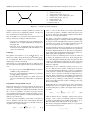
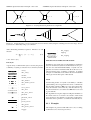
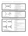
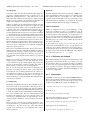
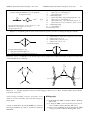
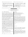
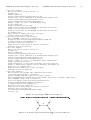
CERN Computer Newsletter 220 April – June 1995
22CERN Computer Newsletter 220 April – June 1995
22
6. Text Processing
6.1 Drawing Feynman Diagrams with LATEX and METAFONT.
Part 1: Design and Basic Usage
Thorsten Ohl (TH Darmstadt, Theoretical High Energy Physics Group)
e-mail: [email protected]
Abstract
LAT
This is the first article in a series describing the EX package feynMF for easy drawing of professional quality Feynman diagrams with METAFONT (or MetaPost). This time
the design principles and the basic usage will be discussed.
In this series of tutorials, I will describe such a system,
feynMF [7], which is completely portable among TEX installations. It is unique among packages for drawing Feynman
diagrams in combining the following features:
• Simplicity and conciseness for common diagrams. For
example, the ubiquitous Z-diagram at LEP1 energies
shown in figure 6.1 can be specified completely in eight
short lines of LATEX. It is never necessary to draft the
diagram on graph paper or to perform calculations to
determine the position of vertices manually.
• Expressiveness for arbitrarily complex diagrams (see
the examples below).
• Extensibility.
• Portability. No graphics devices are needed beyond a
standard TEX installation.
• Arbitrary TEX-labels.
6.1.1 Introduction
In recent years, TEX [1] and LATEX [2] (or other macro packages for structured markup on top of TEX) have revolutionized the way we exchange information in physics (and other
areas). Not only does TEX provide unrivaled typographical capabilities, TEX documents are also completely portable
among essentially all computers in use in the physics community.
TEX’s portability comes with a price, though. It does not address the issue of graphical information, apart from the rudimentary (but very useful) capabilities of the LATEX picture
environment and similar packages [3]. The inclusion of separate graphics files in the PostScript [4] page description language is currently the de facto standard for more complex
graphics.
Handling graphics in an environment completely different
from the (TEX) text environment causes other problems. The
fonts used for labelling graphs will sometimes not blend
smoothly with the fonts used in text and equations. More importantly, these fonts usually lack the ability to create complex mathematical expressions. Finally, external tools are far
less portable than TEX itself.
There are a couple of tools available that address one or more
of the above points in the context of drawing Feynman diagrams. Michael Levine’s feynman package [5] is implemented on top of the standard LATEX picture environment.
This makes it completely portable, but the graphics output is
necessarily less than perfect. Some complex diagrams can
not be produced at all. Jos Vermaseren’s axodraw package [6] uses \special to access PostScript primitives for
drawing diagrams. This approach is very flexible and produces visually more appealing results. Both packages take no
advantage of the formal structure of Feynman graphs, but require the user to specify the layout manually using rather low
level graphics primitives instead.
It is possible to go one step further and move from low-level
tools working on points and curves to a high-level markup
system working on the mathematical structure of graphs.
This step will free the user from having to think about the layout and allow him to concentrate on the structure of the graph
instead.
In the first part of this series, I will concentrate on the “graph
mode” of feynMF, which can be used without having to
learn any METAFONT concepts. Information on how to run
METAFONT is available from Michel Goossens’s tutorial in
section 6.2.1 on page 28 of this CNL. All examples can be
used immediately if saved to a file and enclosed in a
\documentclass{article}
\usepackage{feynmf}
\begin{document}\setlength{\unitlength}{1mm}
\begin{fmffile}{samplepics}
and
\end{fmffile}
\end{document}
pair. To avoid a clash of the METAFONT and TEX .log files,
the LATEX file must not be named samplepics.tex.
Later parts of this series will explain how simple METAFONT
concepts can be used to create more complex Feynman diagrams.
This short tutorial is not a replacement for the user’s manual [7, 8] where feynMF’s features are described more completely.
6.1.2 Description of the Package
As mentioned in the introduction, feynMF was to meet the
following competing design goals: convenience and ease-ofuse, expressiveness, extensibility, and portability. Extensibility was not a goal in itself but was used to provide an environment where simple building blocks can be used for the
CERN Computer Newsletter 220 April – June 1995
23CERN Computer Newsletter 220 April – June 1995
23
1 \begin{fmfchar*}(40,25)
2 \fmfleft{em,ep}
3 \fmf{fermion}{em,Zee,ep}
4 \fmf{photon,label=$Z$}{Zee,Zff}
5 \fmf{fermion}{fb,Zff,f}
6 \fmfright{fb,f}
7 \fmfdot{Zee,Zff}
8 \end{fmfchar*}
Z
Figure 6.1: S imple Z-production diagram.
straightforward solution of simple problems and can be combined to solve the most complicated problems, once the software system has been mastered by the user.
The reconciliation of convenience and expressiveness was
made possible by providing two different modes:
• graph mode, in which the layout is determined automatically from a simple mathematical description of
the graph, and
• immediate mode, in which the user has complete freedom but at a basic familiarity with METAFONT concepts is recommended.
Languages
The primary user interface is a set of LATEX macros. It is
therefore possible to keep the whole paper, including graphics, in a single file. This is very convenient for exchanging
manuscripts by electronic mail [6].
METAFONT [9] (or alternatively MetaPost [10]) has been
chosen as the low level graphics engine for the following reasons:
• it is part of any reasonable TEX installation, therefore
available to all potential users,
• it has very powerful graphics primitives [9], which allow high quality output, and
• it has built-in linear algebra [9], which can be employed for automatic layout algorithms, as detailed below.
Graph Mode and Algorithmic Layout
Early in the design it was clear that feynMF should accept a
mathematical description of a graph and create the layout of
the corresponding Feynman diagram automatically. It should
also not rely on a database of common topologies, because
such a database will necessarily remain incomplete. A more
general strategy is the definition of a function that will be minimized to give the layout.
feynMF provides commands to place a list of external vertices on “galleries” along the sides of the diagram. The function that is minimized for the layout of internal vertices is a
weighted sum of squared lengths
1X
tij (vi − vj )2 ,
(6.1)
L(v1 , . . . , vn ) =
2 i,j
where i, j run over all connections of vertices. The elements
of the “tension” matrix tij default to 1 and can be used to tune
the layout. Obviously, the resulting equations will be linear
and can be solved by METAFONT.
The effect of the tension parameter can be understood by
imagining the graph as consisting of rubber bands. Changing
the tension of an arc will pull adjacent vertices together or allow them to move apart. As an example, figure 6.2 shows the
effect of varying the tension of one line from 4 to 1/4.
Another example for the tension parameter is provided by the
unsatisfactory result of specifying unit tension everywhere in
the ladder diagram in figure 6.3a. The improved diagram in
figure 6.3b has been drawn with vanishing tension of the arcs,
which will result in straight lines for the stems.
In fact, the effect of vanishing tension can also be achieved
by laying out subgraphs step by step. By freezing the layout of the subgraph excluding the rungs in figure 6.3b first
(cf. fig. 6.3c) and adding the rungs later, we arrive at the same
result. Obviously this procedure can be iterated for graphs of
arbitrary complexity.
While there are also commands to fix the position of a vertex or to shift its position, it turns out that the most effective
way of drawing Feynman diagrams consists in a combination
of the stepwise construction of subgraphs and adjustment of
tensions. User’s discretion is advised in tuning tension parameters. More often than not, the defaults give satisfactory
results that can be made perfect by adjusting the tension of a
single arc or loop. Tuning too many tensions is not likely to
improve the results and can be as time consuming as choosing
the layout manually.
Technically, the most convenient aspect of (6.1) is that minimizing it leads to linear equations, which are easily solved. It
would in principle be possible to investigate improved functions like
X
2
N (v1 , . . . , vn ) =
(vi − vj )2 − δ 2 ,
(6.2)
i,j
which would favour arcs of length δ. However, the prize in
having to solve a system of non-linear equations is certainly
too high, in particular because it will be impossible to prove
that reasonable results will result from all user input.
The method of Lagrange multipliers allows us to specify linear constraints among vertices
vi − vj = dij ,
(6.3)
CERN Computer Newsletter 220 April – June 1995
24CERN Computer Newsletter 220 April – June 1995
tij = 4
tij = 1
24
tij = 1/4
Figure 6.2: V arying the tension parameter of a single line.
a)
b)
c)
Figure 6.3: L adder diagram, versions a) using unit tension for all arcs and b) using the vanishing tension for the rungs. Version
b) can also be obtained by using c) as a skeleton.
while still dealing with linear equations. Therefore we add
the term
X
λij · (vi − vj − dij )
(6.4)
Λ=
i,j
to the “action” (6.1).
:
dbl_wiggly
:
zigzag
:
dbl_zigzag
Immediate Mode and Extension Mechanism
Line Styles
A great variety of different line styles is used by the physics
community. feynMF provides the most common by default:
:
curly
:
dbl_curly
:
dashes
:
dashes_arrow
:
dbl_dashes
:
dbl_dashes_arrow
:
dots
:
dots_arrow
:
dbl_dots
:
dbl_dots_arrow
:
phantom
:
phantom_arrow
:
plain
:
plain_arrow
:
dbl_plain
:
dbl_plain_arrow
:
wiggly
In addition to the graph mode for algorithmic layout that has
just been described, feynMF has an immediate mode to provide the user with maximum flexibility. feynMF also implements an extension mechanism that allows the user to install custom line styles of arbitrary complexity. A detailed
description of immediate mode and the extension mechanism
will be given in the later parts of this tutorial.
Labels
An interesting feature of feynMF is the ability to calculate
optimal label positions in METAFONT and to communicate
this information back to LATEX’s picture environment. Because METAFONT cannot write any other files than its logfile, the information is stored there and TEX macros are used
to parse this file.
The algorithm used is quite simple. It will place all labels on
the outside of the arc or vertex it is associated to. If the result
is not satisfactory, the manual [7, 8] describes explicit placement rules can be specified to overwrite the automatic layout.
6.1.3 Examples
All examples are presented with full source code, no tuning
“behind the scenes” has been performed.
CERN Computer Newsletter 220 April – June 1995
e+
25CERN Computer Newsletter 220 April – June 1995
3 \fmflabel{$e_-$}{i1}\fmflabel{$e_+$}{i2}
4 \fmflabel{$\mu_+$}{o1}
5 \fmflabel{$\nu_{\mu}$}{o2}
6 \fmflabel{$s$}{o3}
7 \fmflabel{$\noexpand\bar c$}{o4}
8 \fmf{fermion}{i1,v1,i2}
9 \fmf{boson,label=$\gamma,,Z$}{v1,v2}
10 \fmf{boson}{v3,v2,v4}
11 \fmf{fermion}{o1,v3,o2}
12 \fmf{fermion}{o4,v4,o3}
13 \fmfdot{v1,v3,v4}\fmfblob{.12w}{v2}
14 \end{fmfgraph*}
c̄
s
γ, Z
νµ
e−
25
µ+
1 \begin{fmfgraph*}(50,30)
2 \fmfleftn{i}{2} \fmfrightn{o}{4}
Figure 6.4: R esonant s-channel contribution.
e+
3 \fmflabel{$e_-$}{i1}\fmflabel{$e_+$}{i2}
4 \fmflabel{$\noexpand\bar c$}{o1}
5 \fmflabel{$\nu_{\mu}$}{o2}
6 \fmflabel{$\mu_+$}{o3}
7 \fmflabel{$s$}{o4}
8 \fmf{boson,label=$\gamma,,Z$}{v1,v2}
9 \fmf{fermion}{i1,v1,i2}
10 \fmf{fermion}{o1,v2,v3,o4}
11 \fmffreeze
12 \fmf{boson}{v3,v4}\fmf{fermion}{o3,v4,o2}
13 \fmfdotn{v}{4}
14 \end{fmfgraph*}
s
µ+
νµ
γ, Z
e−
c̄
1 \begin{fmfgraph*}(50,30)
2 \fmfleftn{i}{2}\fmfrightn{o}{4}
Figure 6.5: S ingly resonant contribution.
f
Z
Z
f
Z
f¯
f¯
f
f
Z
f¯
f¯
1 \newenvironment{Zff}
2 {\begin{fmfgraph*}(35,30)
3
\fmfleft{Z}\fmfright{fb,f}
4
\fmflabel{$\noexpand\bar f$}{fb}
5
\fmflabel{$Z$}{Z}\fmflabel{$f$}{f}}
6 {\end{fmfgraph*}}
7 \begin{Zff}
8 \fmf{boson}{Z,v}\fmf{fermion}{fb,v,f}
9 \fmfdot{v}
10 \end{Zff}
11 \begin{Zff}
12 \fmf{boson}{Z,v1}\fmf{boson}{v2,v3}
13 \fmf{fermion,left,tension=.5}{v1,v2,v1}
14 \fmf{fermion}{fb,v3,f}\fmfdotn{v}{3}
15 \end{Zff}\\[3\baselineskip]
16 \begin{Zff}
17 \fmf{boson}{Z,Zv}
18 \fmf{fermion}{fb,fbv,Zv,fv,f}
19 \fmffreeze
20 \fmf{boson}{fbv,fv}\fmfdot{Zv,fbv,fv}
21 \end{Zff}
22 \begin{Zff}
23 \fmf{boson}{Z,Zv}\fmf{boson}{fbv,Zv,fv}
24 \fmf{fermion}{fb,fbv}\fmf{fermion}{fv,f}
25 \fmffreeze
26 \fmf{fermion}{fbv,fv}\fmfdot{Zv,fbv,fv}
27 \end{Zff}
Figure 6.6: Z-decay at tree level and at one loop
CERN Computer Newsletter 220 April – June 1995
26CERN Computer Newsletter 220 April – June 1995
26
Tree Diagrams
Equations
Let us start with a view into the immediate future: figure 6.4
shows the s-channel diagram for the production of W ’s at
LEP2 with semileptonic decay. The starred form of the
fmfgraph environment is used because we want to include
labels for vertices and arcs. Its arguments are the width and
height of the diagram, measured in \unitlengths.
Feynman diagrams can be used everywhere in a LATEX document, in particular in centered \parboxes for creating graphical equations like the one in figure 6.7. The only new
feynMF feature in this figure is the arc connecting a vertex
with itself in line 6. Such lines do not affect the layout and
feynMF will draw them into the biggest available gap.
In line 2 we declare two incoming particles and four outgoing
particles, which will be placed on the left or right side of the
diagram, respectively. These vertices are labelled in lines 3–
7. On line 7, the \bar command has been protected from premature expansion by \noexpand. This is similar to LATEX’s
moving arguments, but necessary for some robust commands
too. If in doubt, protect all commands; it will never hurt. Line
8 connects the incoming fermions with the first inner vertex.
This vertex is connected in line 9 with the W W γ/Z vertex.
Here it should be noted that the line style (boson in this case,
which is an alias for wiggly) takes comma-separated options.
Here we add a label with the label option. Inside the argument of an option, commas have to be doubled to distinguish
them from option separators.
The rest is now straightforward: lines 10–12 connect the remaining vertices with W ’s and fermions and line 13 add dots
and a blob at the respective vertices. The width of the blob
is specified in the first argument of \fmfblob to be 12% of
the total width of the diagram, 6mm would be as good in this
example.
Figure 6.5 is a variation on that theme, this time showing a
singly resonant contribution to the same final state. Lines
3–7 are identical to the preceding diagram, but permute the
flavours of the final states. In lines 8–10 the outer string of
fermion lines is connected to the incoming particles.
Line 11 uses the important \fmffreeze command for the
first time. It will fix the layout of the vertices that have
been entered so far, producing a skeleton for the vertices entered later. If we would no do this, the W and fermions entered in line 12 would pull the diagram over to the right too
much (try this by processing the diagram with and without the
\fmffreeze yourself!).
Loop Diagrams
Returning to the physics currently produced at LEP, we show
the tree-level and one-loop diagrams contributing to the decay of Z’s into two fermions in figure 6.6. Since we will have
to produce four diagrams with identical external particles, it is
convenient to define an environment in lines 1–6 that will take
care of the repetitive tasks. The rest of the example should
be almost self-explanatory by now. Let me just point to the
\fmffreeze commands in lines 19 and 25 that are used to
obtain a straight continuation of the external arcs into the triangles.
Line 13 uses the tension option to reduce the tension of the
ares in the fermion loop, effectively blowing up the loop from
its default size. Also new is the left option that instructs
feynMF not to draw the arc on a straight line, but to take a
left detour instead.
Multi-loop Diagrams
Multi-loop diagrams can pose special challenges: in figure 6.8 two renditions of a O(αS α) contribution to the Zselfenergy are shown. The first uses graph mode commands
exclusively but its visual appearance is certainly inferior to
the second version that uses immediate mode commands to
generate arcs that are more generally curved than half-circles.
The full source code of this version will be discussed in the
next issue of the CNL.
In the graph mode version, we note the first use of the
\fmffixed command which is used to specify a linear constraint (cf. (6.3)). If this command were not be used, the loop
would collapse, therefore we force it open by demanding that
the upper vertex vn be exactly the full height of the diagram
above the lower vertex vs: vn − vs = (0, h).
6.1.4 Conclusion and Outlook
The examples that have been presented in this first part of the
tutorial were selected with the aim of providing a very gentle introduction. They do not exhaust feynMF’s capabilities
by far. Some more advanced applications will be discussed
in two sequels to this article. Among the examples described
in detail will be the “penguin” diagram and the Higgs production process of figure 6.9.
6.1.5 Distribution
At CERN, feynMF is part of the standard LATEX installation.
Readers from institutions that have not yet installed feynMF,
can get the latest release by anonymous ftp from any of the
Comprehensive TEX Archive Network (CTAN) hosts
ftp.shsu.edu, ftp.tex.ac.uk, ftp.dante.de
in the directory
macros/latex/contrib/supported/feynmf
Important announcements (new versions, fatal bugs, etc.)
will be made through the mailing list
[email protected]
Subscriptions can be obtained from
[email protected]
CERN Computer Newsletter 220 April – June 1995
27CERN Computer Newsletter 220 April – June 1995
In supersymmetrical field theories, the quadratic
divergences cancel:
= ln Λ2
+
(6.5)
1 In supersymmetrical field theories, the
2 quadratic divergences cancel:
3 \begin{equation}
27
4 \parbox{20mm}{\begin{fmfgraph}(20,15)
5
\fmfleft{i} \fmfright{o}
6
\fmf{dashes}{i,v,v,o}
7 \end{fmfgraph}}
8 + \parbox{20mm}{\begin{fmfgraph}(20,15)
9
\fmfleft{i} \fmfright{o}
10
\fmf{dashes}{i,v1} \fmf{dashes}{v2,o}
11
\fmf{fermion,left,tension=.3}{v1,v2,v1}
12 \end{fmfgraph}}
13 = \ln\Lambda^2
14 \end{equation}
Figure 6.7: G raphical equations can be created easily, the \parbox is used for centering the diagram vertically.
4 \fmf{fermion,tension=.5}{vw,vn,ve,vs,vw}
5 \fmf{gluon}{vn,vs}
6 \fmffixed{(0,h)}{vn,vs}
7 \fmfdot{vw,vn,ve,vs}
8 \end{fmfgraph}
1 \begin{fmfgraph}(50,20)
2 \fmfleft{w}\fmfright{e}
3 \fmf{boson}{w,vw}\fmf{boson}{ve,e}
Figure 6.8: O(αS α) contribution to the Z-selfenergy, both in a graph mode rendition and and in an improved version that
needs immediate mode commands.
H
b
s
W
t
t
g(x1 , Q2 )
P1
x1 P 1
x2 P 2
g(x2 , Q2 )
P2
Figure 6.9: A “penguin” diagram in fancy layout and a Higgs production process. These examples will be discussed in the
next article of this series.
(send a message consisting of help to majordomo for instructions on how to subscribe, don’t send such messages to
the list itself).
feynMF is distributed in the standard LATEX doc format [3].
The simple installation procedure is described in detail in a
README file.
Bibliography
[1] D. E. Knuth, The TEXbook (Addison-Wesley, Reading,
MA, 1986).
[2] L. Lamport, LATEX — A Document Preparation System,
2nd ed. (Addison-Wesley, Reading, MA, 1994).
[3] M. Goossens, F. Mittelbach, and A. Samarin, The LATEX
Companion (Addison-Wesley, Reading, MA, 1994).
CERN Computer Newsletter 220 April – June 1995
28CERN Computer Newsletter 220 April – June 1995
[4] Adobe Systems Incorporated, PostScript Language
Reference Manual, 2nd ed. (Addison-Wesley, Reading,
MA, 1990).
[5] M. J. S. Levine, Comp. Phys. Comm. 58, 181 (1990).
[6] J. Vermaseren, Comp. Phys. Comm. 83, 45 (1994).
[7] T. Ohl, Preprint IKDA 95/20, hep-ph/9505351, TH
Darmstadt (unpublished).
[8] T. Ohl, feynMF user’s manual, 1995, TEX
28
file accompanying the distribution. At CERN
the manual can be found in the directory
/usr/local/doc/tex/feynmf-1.0/ as the gzipped
PostScript file manual.ps.gz.
[9] D. E. Knuth, The METAFONTbook (Addison-Wesley,
Reading, MA, 1986).
[10] J. D. Hobby, Computer Science Report 162, AT&T Bell
Laboratories (unpublished).
6.1.1 6.1.1 6.1.1, 6.1.5 6.1.1 6.1.1 6.1.1, 6.1.2 6.1.1, 6.1.1, 6.1.2 6.1.1, 6.1.2 6.1.2, 6.1.2, 6.1.2 6.1.2
6.2 A short introduction to METAFONT
Michel Goossens CN/ASD
6.2.1 What is METAFONT?
METAFONT is a program for making bitmap fonts for use
by TEX, its viewers, printer drivers, and related programs. It
interprets a drawing language with an Algol-like syntax and
uses third-order Bernstein polynomials to parametrize curve
segments. In contrast, the other well-known drawing language, PostScript, is stack-based and uses third-order Bézier
curves to represent curve segments. Both are actively used to
draw pictures (see previous article) and fonts (type1-fonts for
PostScript, Knuth’s well-known Computer Modern METAFONT family, the default font used with TEX).
METAFONT source files are usually suffixed ‘.mf’. METAFONT allows scaling, rotation, reflection, skewing and shifting, and other complex transformations.
METAFONT’s bitmap output is a gf (generic font) file, that
can be compressed into an equivalent pk (packed) format
by the auxiliary program gftopk. These file are characterized by the suffixes “.*gf” and “.*pk” respectively, where,
on U NIX installations, the “*” stands for the font resolution, while on MS - DOS, with its three-character limit on suffix
length, a suffix like “.2540gf” will become “.240”. On top
of that, for TEX to typeset a font it needs a tfm (TEX font metrics) file to describe the dimensions, ligatures and kerns of the
font in a device-independent way. In general, unless one is
using proof mode (see below), METAFONT will always create a tfm file. Note that, since TEX only reads the tfm files,
the actual glyphs, or forms of the characters, as stored in gf
or pk files, are only needed by the DVI-drivers when they produce viewable output.
TEX can scale the information in the tfm files, but the glyphs
in the bitmap files are not scalable. One should use METAFONT to generate the bitmap images at the correct size and
resolution, as explained below.
6.2.2 Interacting with METAFONT
In principle, to run the METAFONT program it is enough to
call it and give it some instructions, as follows:
> mf
This is METAFONT, Version 2.71 (C version 6.1)
**\mode=qms;
*input logo10
(/usr/local/lib/texmf/mf/plain/logo10.mf
(/usr/local/lib/texmf/mf/plain/logo.mf
[77] [69] [84] [65] [70] [80] [83] [79] [78]) )
Font metrics written on mfput.tfm.
Output written on mfput.300gf
(9 characters, 1120 bytes).
Transcript written on mfput.log.
The first line with the “**” prompt tells us that METAFONT
is waiting for input. At that point we indicate for which device we want to generate bitmapped fonts (see above) by using the \mode command followed by a name that should be
known by METAFONT (your local system administrator for
the TEX system has most probably installed a few commonly
user output devices when creating the executable). When in
doubt you can always ask METAFONT about the known devices by typing the following after the ** prompt (only a very
partial list is shown for the U NIX installation at CERN):
> mf
This is METAFONT, Version 2.71 (C version 6.1)
**\relax
*?
proof_
...
qms_
...
XeroxDocutech_
*bye
In general, and in particular at CERN, the system administrator has chosen a “default” font mode for use at that installation. In this case one can specify the localfont mode:
> mf ’\mode=localmode; input logo10;’
At CERN the “CanonCX”, a 300 dpi engine, was chosen
as a default. In the above example it is also seen that one
can also specify all METAFONT commands on the command
line, quoting the complete string so that it is not interpreted
by the shell. For higher resolutions (above 600 dpi or so) one
will have to find the mode corresponding to the device one
wants to use, e.g.,
CERN Computer Newsletter 220 April – June 1995
29CERN Computer Newsletter 220 April – June 1995
> mf ’\mode=XeroxDocutech; input logo8;’
This is METAFONT, Version 2.71 (C version 6.1)
(/usr/local/lib/texmf/mf/plain/logo8.mf
(/usr/local/lib/texmf/mf/plain/logo.mf
[77] [69] [84] [65] [70] [80] [83] [79] [78]) )
Font metrics written on logo8.tfm.
Output written on logo8.600gf
(9 characters, 1600 bytes).
Transcript written on logo8.log.
If METAFONT cannot find a file, one can either enter the correct file name, or else type the name null.tex, that will get
METAFONT back into input mode, and then exit with the bye
command.
Sometimes users get into trouble when specifying no or an
unknown mode, and obtain filenames of the type *.2602gf.
On U NIX running X-Window, there will also appear large
characters on-screen. This behaviour corresponds to METAFONT’s “proof” mode, used by font designers to have a
magnified view of their fonts at a resolution of 2601.72 dpi—
36 pixels per point (hence the 2602 file extension).
> mf
This is METAFONT, Version 2.71 (C version 6.1)
**\input logo10.mf
(/usr/local/lib/texmf/mf/plain/logo10.mf
(/usr/local/lib/texmf/mf/plain/logo.mf
[77] [69] [84] [65] [70] [80] [83] [79] [78]) )
Output written on logo10.2602gf
(9 characters, 9880 bytes).
Transcript written on logo10.log.
29
6.2.3 Locating files
An often-occurring problem is the one where TEX or METAFONT (and their helper programs) do not find the necessary
files (or one wants to instruct them to look in supplementary
directories). The TEX-related programs, as set up at CERN,
refer to system variables shown in the table below.
TEX, METAFONT, BIBTEX, and MakeIndex
Type of file
System variable
TEX pool
TEXPOOL
TEX formats
TEXFORMATS
TEX inputs
TEXINPUTS
TEX tfm
TFMFONTS, TEXFONTS
METAFONT pool
MFPOOL
METAFONT bases
MFBASES
METAFONT inputs MFINPUTS
BIBTEX bst
BSTINPUTS, TEXINPUTS
BIBTEX bib
BIBINPUTS
MakeIndex ist
INDEXSTYLE
They are initialized to look in the current and certain systemwide directories. One can add one’s own directories by writing, for instance in the U NIX Bourne shell (or something
equivalent in other shells or operating systems):
TEXINPUTS=/user/goossens/mytexfiles:
export TEXINPUTS
MFINPUTS=/user/goossens/mymffiles:
export MFINPUTS
In this case it is enough to specify the correct mode.
Magnification (and Resolution)
As TEX works with font sizes increasing in geometric ratios
(so-called “magsteps”, which go in steps of 1.2), one can
specify values for those magsteps to METAFONT, e.g.,
> mf
This is METAFONT, Version 2.71 (C version 6.1)
**\mode=localfont; mag=magstep(1); input logo10;
(/usr/local/lib/texmf/mf/plain/logo10.mf
(/usr/local/lib/texmf/mf/plain/logo.mf
[77] [69] [84] [65] [70] [80] [83] [79] [78]) )
Font metrics written on logo10.tfm.
Output written on logo10.360gf
(9 characters, 1284 bytes).
Transcript written on logo10.log.
As seen, one now gets a font of type .360gf, that is 1.2×300.
To make the pk packed font bitmap file needed by the various
DVI-drivers, one should run the gftopk program, as follows:
> gftopk -v logo10.360gf
This is GFtoPK 2.3 (C version d)
[./logo10.360gf->logo10.360pk]
’METAFONT output 1995.06.13:0856’
1284 bytes packed to 580 bytes.
Without the -v option, gftopk runs silently. Note the size of
the pk file that is about twice smaller then the original gf file.
Here TEX and METAFONT are instructed to first look
in the directories /user/goossens/mytexfiles and
/user/goossens/mymffiles, before looking in the
compiled-in default directories (symbolized by the colon
“:” at the end of the path), i.e.,at CERN, the current directory followed by /usr/local/lib/texmf/tex and /usr/
local/lib/texmf/mf. Similarly, the next table shows the
variables controlling the behaviour of dvips.
Type of file
dvi files
pk fonts
virtual fonts vf
configuration files config.*
PostScript files
MakeTeXPK script
System variable
current directory
DVIPSFONTS, TEXPKS,
PKFONTS, TEXFONTS
VFFONTS, TEXFONTS
TEXCONFIG
TEXINPUTS
MAKETEXPK
MakeTeXPK
On U NIX, when fonts are missing, the dvips and xdvi DVIprograms call a Bourne shell script, “MakeTeXPK”, which creates a temporary directory, which it then changes, before calling METAFONT to generate the missing fonts. This is shown
below in the case of xdvi in Figure 6.10 on page 30, where the
missing font bitmap file cmrtt12 at a magstep of 21 was generated automatically by xdvi.
CERN Computer Newsletter 220 April – June 1995
30CERN Computer Newsletter 220 April – June 1995
30
>>>[1] xdvi kpathsea
kpathsea: Running MakeTeXPK cmtt12 329 300 magstep\(0.5\)
/usr/local/bin/MakeTeXPK: Running virmf \mode:=CanonCX;
mag:=magstep(0.5); scrollmode; input cmtt12
This is METAFONT, Version 2.71 (C version 6.1)
(/usr/local/lib/texmf/fonts/cm/src/cmtt12.mf
(/usr/local/lib/texmf/fonts/cm/src/cmbase.mf)
(/usr/local/lib/texmf/fonts/cm/src/roman.mf
(/usr/local/lib/texmf/fonts/cm/src/romanu.mf [65] [66] [67] [68] [69] [70] [71] [72] [73]
[74] [75] [76] [77] [78] [79] [80] [81] [82] [83] [84] [85] [86] [87] [88] [89] [90])
(/usr/local/lib/texmf/fonts/cm/src/romanl.mf [97] [98] [99] [100] [101] [102] [103] [104] [105]
[106] [107] [108] [109] [110] [111] [112] [113] [114] [115] [116] [117] [118] [119] [120] [121] [122])
(/usr/local/lib/texmf/fonts/cm/src/greeku.mf [0] [1] [2] [3] [4] [5] [6] [7] [8] [9] [10])
(/usr/local/lib/texmf/fonts/cm/src/romand.mf [48] [49] [50] [51] [52] [53] [54] [55] [56] [57])
(/usr/local/lib/texmf/fonts/cm/src/romanp.mf [36] [38] [63] [15])
(/usr/local/lib/texmf/fonts/cm/src/romspl.mf [16] [17] [25] [26] [27] [28])
(/usr/local/lib/texmf/fonts/cm/src/romspu.mf [29] [30] [31])
(/usr/local/lib/texmf/fonts/cm/src/punct.mf [33] [14] [35] [37] [39] [40] [41] [42] [43] [44] [46]
[47] [58] [59] [61] [64] [91] [93] [96])
(/usr/local/lib/texmf/fonts/cm/src/accent.mf [18] [19] [20] [21] [22] [23] [24] [94] [126] [127])
(/usr/local/lib/texmf/fonts/cm/src/romsub.mf
(/usr/local/lib/texmf/fonts/cm/src/sym.mf [45] [12] [11] [60] [62] [95] [92] [124] [123] [125]
[34]) [13] [32]) ) )
Font metrics written on cmtt12.tfm.
Output written on cmtt12.329gf (128 characters, 13856 bytes).
Transcript written on cmtt12.log.
created /user/goossens/pk/CanonCX/cmtt12.329pk
Figure 6.10: A utomatic generation of font bitmaps by MakeTeXPK
6.2.4 Running METAFONT with feynmf
Figure 6.11 on page 30 shows a small input file (with an example taken from Thorsten Ohl’s article) using the feynmf
package. Figure 6.12 on page 31 shows the whole procedure
of obtaining printable output from the given input. One first
runs LATEX (line >>>[1]) to generate files that METAFONT
will translate in gf files (line >>>[2]). A second LATEX run
(line >>>[3]) then uses the information in those files to enter in the DVI-file code that can be transformed into the de-
sired printable form. To generate PostScript output, dvips is
run (line >>>4) and it is seen how that program calls upon the
MakeTeXPK script (just like xdvi, as shown in Fig. 6.10) to
generate the pk bitmap of the Feynman image, that is then included into the final PostScript output file, shown in Fig. 6.13
on page 31.
Let me mention that there now exists a program MetaPost,
that has a functionality similar to METAFONT, but it generates PostScript output directly. An article in the next issue of
the CNL will explain the basics of that program.
\documentclass{article}
\usepackage{feynmf}
\begin{document}
\setlength{\unitlength}{1mm}
An example of a Feynman graph drawn with Thorsten Ohl’s \texttt{feynmf} package.
\begin{center}
\begin{fmffile}{feynexa}
\begin{fmfchar*}(40,25)
\fmfleft{em,ep}
\fmf{fermion}{em,Zee,ep}
\fmf{photon,label=$Z$}{Zee,Zff}
\fmf{fermion}{fb,Zff,f}
\fmfright{fb,f}
\fmfdot{Zee,Zff}
\end{fmfchar*}
\end{fmffile}
\end{center}
\end{document}
Figure 6.11: LATEX source file with a simple example of a Feynman diagram
CERN Computer Newsletter 220 April – June 1995
31CERN Computer Newsletter 220 April – June 1995
>>>[1] latex feynmfex
This is TeX, Version 3.1415 (C version 6.1)
(feynmfex.tex
LaTeX2e <1994/12/01>
(/usr/local/lib/texmf/tex/latex/base/article.cls
Document Class: article 1994/12/09 v1.2x Standard LaTeX document class
(/usr/local/lib/texmf/tex/latex/base/size10.clo))
(/usr/local/lib/texmf/tex/latex/feynmf/feynmf.sty
Package: ‘feynmf’ v1.0 (rev. 1.12) <1995/05/06> (ohl))
No file feynmfex.aux.
feynmf: File feynexa.tfm not found:
feynmf: Process feynexa.mf with METAFONT and then reprocess this file.
feynmf: Label file feynexa.t1 not found:
feynmf: Process feynexa.mf with METAFONT and then reprocess this file.
[1] (feynmfex.aux) )
Output written on feynmfex.dvi (1 page, 388 bytes).
Transcript written on feynmfex.log.
>>>[2] mf "\mode=localfont; \input feynexa"
This is METAFONT, Version 2.71 (C version 6.1)
(feynexa.mf (/usr/local/lib/texmf/fonts/feynmf/src/feynmf.mf)
:1:\fmfL(19.98138,14.59717,b){$Z$}% [1] )
Font metrics written on feynexa.tfm.
Output written on feynexa.300gf (1 character, 2184 bytes).
Transcript written on feynexa.log.
>>>{3] latex feynmfex
This is TeX, Version 3.1415 (C version 6.1)
(feynmfex.tex
LaTeX2e <1994/12/01>
(/usr/local/lib/texmf/tex/latex/base/article.cls
Document Class: article 1994/12/09 v1.2x Standard LaTeX document class
(/usr/local/lib/texmf/tex/latex/base/size10.clo))
(/usr/local/lib/texmf/tex/latex/feynmf/feynmf.sty
Package: ‘feynmf’ v1.0 (rev. 1.12) <1995/05/06> (ohl)) (feynmfex.aux)
feynmf: File feynexa.tfm found.
feynmf: Nevertheless, if the picture has changed, reprocess feynexa.mf.
feynmf: If dimension have changed, reprocess feynexa.mf and feynmfex.tex.
(feynexa.t1) [1] (feynmfex.aux) )
Output written on feynmfex.dvi (1 page, 476 bytes).
Transcript written on feynmfex.log.
>>>[4] dvips feynmfex -o
This is dvipsk 5.58e Copyright 1986, 1994 Radical Eye Software
’ TeX output 1995.06.06:1756’ -> feynmfex.ps
kpathsea: Running MakeTeXPK feynexa 300 300 1+0/300 CanonCX
/usr/local/bin/MakeTeXPK: Running virmf \mode:=CanonCX; mag:=1+0/300; scrollmode; input feynexa
This is METAFONT, Version 2.71 (C version 6.1)
(/afs/.cern.ch/project/cnas_doc/sources/cnl/220/feynexa.mf
(/usr/local/lib/texmf/fonts/feynmf/src/feynmf.mf)
:1:\fmfL(19.98138,14.59717,b){$Z$}% [1] )
Font metrics written on feynexa.tfm.
Output written on feynexa.300gf (1 character, 2184 bytes).
Transcript written on feynexa.log.
created /user/goossens/pk/CanonCX/feynexa.300pk
<tex.pro>. [1]
Figure 6.12: T ypesetting the LATEX job shown in Fig. 6.11
!"#!%$'&)(" *& +,.-/*102
3450"
67
8
9
Figure 6.13: P ostScript output generated from the LATEX source shown in Fig. 6.11
31