Download FDEMINV

FDEMINV
1-D interpretation of frequency-domain EM soundings
Version 1.4a (c) 2012 by Markku Pirttijärvi
Introduction:
The FDEMINV program can be used to model and to interpret geophysical frequency-domain
electromagnetic (FDEM) soundings over horizontally layered earth. FDEMINV can compute
various magnetic field responses derived from the vertical and the horizontal component of the
magnetic field due to a vertical and/or a horizontal magnetic dipole. Parameter optimization, which
is based on linearized inversion method, can be utilized in 1-D interpretations.
The FDEMINV program is a 32-bit application that can be run on Windows 9x/XP/7 with a
graphics display of at least 1024800 resolution. Memory requirements and processor speed and
are not critical factors, since large data arrays are not used and the EM solution is quite fast to
compute even on older computers. The FDEMINV program has a simple graphical user interface
(GUI) that can be used to change the parameter values, to handle file input and output, and to
visualize the EM response and the model. The user interface and the data visualization are based on
the DISLIN graphics library (http://www.dislin.de).
Despite its inversion capabilities, FDEMINV is intended primarily for forward modeling and
testing. One of the main reasons for me to create this program was to develop a general method to
transform FDEM responses into apparent resistivity and phase using the vertical and horizontal
magnetic field components and to test the transformation.
Installing the program:
The program requires following files:
FDEMINV.EXE
the 32-bit executable file
DISDLL.DLL
dynamic link library for the DISLIN graphics
The distribution file (FDEMINV.ZIP) contains also a short description file (_README.TXT), this
user's manual (FDEMINV_MANU.PDF) and an example data file (EXAMPLE.DAT). To install
the program, create a new directory and copy or unzip the distribution files there. To be able to start
the program from a shortcut that locates in a different directory move or copy the DISLIN.DLL file
into the WINDOWS\SYSTEM folder or someplace else where a system path has been defined.
The EM measurement systems:
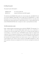
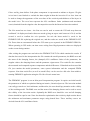
Figure 1 illustrates the three measurement systems considered in FDEMINV. The transmitter, Tx, is
either a vertical (VMD) or a horizontal (HMD) magnetic dipole (that is to say a horizontal or a
vertical loop) on or above the ground surface. The receiver, Rx, is located at the same height level
at some distance, L, away from the source. The FDEMINV program computes two magnetic field
components. The first component (solid black arrow) is always parallel to the source dipole and the
second one (dashed gray arrow) is perpendicular to that. In case of VMD the second component is
the horizontal (axial) component directed away from the source. In case of a HMD source, the
second component is the vertical one. Please, note that in coaxial HMD configuration no vertical
field is generated, which prevents computation of Hx/Hz, Hz/Hx ratios and apparent resistivity and
phase.
2
Tx
Rx
VMD (coplanar)
L
Rx
Tx
HMD (coplanar)
L
Tx
Rx
HMD (coaxial)
L
Figure 1. Schematic view of the commonly used VMD and HMD systems.
The FDEMINV program can be used to model both frequency and geometric soundings. In
frequency soundings the distance between the source and the receiver is kept fixed and the
measurements are made using varying frequencies. The attenuation of EM fields depends on the
conductivity (or its reciprocal, the resistivity) and the frequency. Therefore, high frequencies give
information about the upper parts of the earth, whereas low frequency data contains information
from greater depths. In geometric soundings the frequency is kept fixed and the loop spacing is
varied. When the loop spacing is short the data contains information near the surface. When the
loop spacing increases more and more information will be obtained from the deeper parts of the
earth. For more detailed information about the geophysical EM measurement systems, please, be
referred to common geophysical literature (e.g., M.N. Nabighian, 1988 & 1991, SEG).
The FDEMINV program computes the apparent resistivity and phase using the ratio of the vertical
and horizontal magnetic field components. Although similar method has been used in the French
BRGM Melis frequency sounding system, for example, the method is not widely used and therefore
a short description is provided in the following. The 10-base logarithm of the imaginary
(quadrature) part of the ratio of vertical and horizontal magnetic field (F= Log10(Abs(Im(Hz/Hx))))
is first computed and tabulated using the homogeneous half-space model over a wide range of
dimensionless induction parameter = k2r2, where r is the loop spacing and k2= h (= 2f is
3
angular frequency,  is magnetic permeability of the free-space and h is the conductivity of the
lower half-space). In practice the computation is made using fixed loop spacing and frequency and
varying the host conductivity (or resistivity) values.
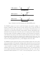
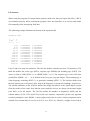
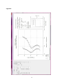
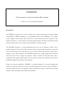
Figure 2 illustrates the F-ratio for a VMD system on the surface of homogeneous half-space. Since
the F-ratio is a continuously decreasing function of the induction parameter, the apparent resistivity
of the VMD (or HMD) system above layered earth can be obtained using reverse interpolation. Let
us assume that at some frequency the computed (or measured) values of vertical and horizontal
magnetic field are Hxi and HzI, which gives rise to ratio Fi. Reverse interpolation (from y- to x-axis)
of the curve shown in Figure 2 gives an induction parameter value, i. In practice the interpolation
is made using the log10 values of the induction parameter and linear extrapolation is used beyond
the computed range if necessary. By its definition the apparent resistivity is such a value of the
resistivity (or conductivity) of the homogeneous half-space that produces the same EM response as
the layered earth. Since the loop spacing and frequency are known, the host conductivity, which
now represents the apparent resistivity can be solved simply as  a  2 0 f  r 2 i (Ohmm). The
phase response related to the apparent resistivity is computed in the FDEMINV program as
  tan 1 ImHz Hx, ReHz Hx (rad. or deg.).
Figure 2. The F-ratio used to interpolate the apparent resistivity for a VMD source
on the surface of homogeneous halfspace.
4
Note that the method used to compute apparent resistivity could be used to transform measured
data as well. This requires, however, that both the vertical and the horizontal magnetic field have
been measured. The transformation method works with coplanar HMD system, which has an Fratio curve very similar to that in Figure 2. Note also that the magnetic field used to compute the Fratio is the sum of free-space and homogeneous half-space magnetic fields and for some dipoledipole systems the vertical magnetic field is zero. Therefore, the interpolation of the F-ratio cannot
be used to compute the apparent resistivity for the coaxial HMD system, for example.
Using the program:
On startup the program reads the model parameters from the FDEMINV.INP file and the DISLIN
graphics parameters from the FDEMINV.DIS file. If these files can not be found when the program
starts, new ones are created automatically using the default parameter values. The program then
computes the FDEM response of the initial model and builds up the user interface shown in the
Appendix. The FDEM response is plotted in the graph area along with a resistivity-depth curve of
the model and a description of the model parameters. The parameters of the layered earth model
and the inversion method can be altered using the controls on the left side of the FDEMINV
program window.
As shown in Appendix the main window of the FDEMINV application contains two menus. The
File menu has the following nine options:
Open Model
open an existing model file (*.INP).
Save Model
save the model into a file (*.INP).
Read Data
read in measured data for interpretation (*.DAT).
Save Results
save the results into a file (*.OUT).
Read disp.
read in new graph parameters from a file (*.DIS).
Save Graph as PS
save the graph in Adobe's Postscript format (*.PS).
Save Graph as EPS
save the graph in Adobe's Encapsulated Postscript format (*.EPS).
Save Graph as PDF
save the graph in Adobe's Acrobat PDF format (*.PDF).
Save Graph as WMF
save the graph in Windows metafile format (*.WMF).
5
Selecting these menu options brings up a typical Windows file selection dialog that can be used to
provide the name of the file for open/save operation. Model and result files are saved in standard
ASCII text format. The graphs are saved as they appear on the screen in landscape A4 size.
The Edit menu contains following items:
Comp.->Meas.
use the computed response as measured data.
Remove Meas.
remove information about measured data.
Sounding type
choose between frequency and geometric .
Source type
choose between coplanar VMD and HMD and coaxial HMD system
Field component
select real & imaginary (in-phase and quadrature) and modulus & phase
response of the first or second (H1 or H2) field components (see note).
Normalized field
select Re,Im and Mod,Pha response of the normalized field (H1/H0) or
(H2/H0), where H0 is primary free-space field (see note).
Ratio
select Re,Im and Mod,Pha response of the ratio between first and
second field component (H1/H or H2/H1).
Apparent resistivity
select apparent resistivity and phase (between H1 and H2) response.
Free space field
include or exclude the free-space field from the total magnetic field
Response component
show either both components or only the first or second component
Note: In case of the VMD source the first field component is vertical magnetic field and the second
is horizontal (axial) magnetic field. In case of HMD the first field component is horizontal (parallel
or coaxial) horizontal magnetic field and the second is the vertical magnetic field, which cannot be
computed in case of coaxial HMD configuration. Consequently, the normalizing free-space
magnetic field H0 is the vertical for VMD source and horizontal for HMD source.
Define freq/dist item can be used to set the minimum and maximum frequency values and number
of frequencies in case of frequency soundings or the minimum and maximum loop spacing and the
number of loop spacings in case of geometric sounding. The values are provided using an input
dialog and the frequencies or loop spacings are automatically computed so that they are evenly
spaced on a logarithmic scale.
6
Phase rad/deg item defines if the phase component is represented as radians or degrees. Weights
in/out item is used include or exclude the data weights in/from the inversion. Error bars item can
be used to change the appearance of the error bars of the resistivity and thickness of the layers in
the model view. The error bars represent the 95% confidence limits (minimum and maximum
errors) obtained from the singular value decomposition used in the linearized inversion method.
The Exit menu has two items - the first one can be used to restart the GUI and swap between
traditional 3:4 display mod and widescreen mode (giving an aspect ratio between 0.5-0.9) and the
second is used to confirm the exit operation. On exit the latest model is saved in the
FDEMINV.INP file replacing the original one, and the results are saved in the FDEMINV.OUT
file. Errors that are encountered before the GUI starts up are reported in the FDEMINV.ERR file.
When operating in GUI mode, run-time errors arising from illegal parameter values are displayed
on the screen during runtime.
After exiting the program one can look at the FDEMOUT.OUT file which contains the results. If
data has been used in the interpretation the file contains the model parameters, the RMS error and
the mean of the damping factors, the (damped) 95% confidence limits of the parameters, the
singular values, the damping factors and the parameter eigenvectors. The result file also contains
the measured and computed response components and the differences. If data had not been used the
file just contains the model parameters, some system information and the computed FDEM
response. Note that result files (as well as model files) can be saved to disk also from within a
running FDEMINV application using the File/Save Results menu item.
The FDEMINV program is not an idiot-proof interpretation program. It requires an initial model,
the parameters of which are optimized during an iterative, linearized process. The inversion method
can easily get stuck to a local minimum, and therefore, the user should pay attention to the validity
of the resulting model. The RMS error and the mean of the damping factors can be used to assess
the validity of the inversion results. Optimally the RMS error should be zero and all damping
factors should be equal to one. Note also that after optimization the resistivity-depth section shows
the minimum and maximum parameter ranges using dotted lines. These auxiliary curves are
derived from the 95% confidence limits.
7
Program controls:
The leftmost control panel includes some push-button and text-field controls. The Loop/Freq text
field defines the loop spacing (when modeling frequency sounding) or the frequency (when
modeling geometric sounding). The value of the loop spacing or frequency is given multiplied by
one thousand (in km or kHz). The other text-fields are used to provide the number of layers and the
resistivity and thickness values of each layer. After editing the parameter values one has to apply
for the changes using the Update parameters push button in the top left corner of the FDEMINV
application window. When increasing or decreasing the number of layers the unnecessary text-field
controls get hidden. The maximum number of layers is six (6). The Default pushbutton resets all
layer parameters to their default values (100 m and 100 m).
The text controls in the right control panel are related to the inversion. These controls become
active only after some data is read in using the File/Read Data item. The Iters. text field control
defines the number of successive iteration made after the Optimize button is pressed. The Thres.
control defines the minimum singular value threshold used in the optimization. This parameter
(actually multiplied by 1000) controls the strength of the damping. Decreasing its value will loosen
the damping and make the inversion method work more like a steepest descent algorithm.
Increasing its value might be advantageous if the inversion gets unstable. The default values of the
iteration number and threshold are 10 and 1.0 (1.e-3), respectively.
The text fields (Free) on the right side of each resistivity and thickness value are used to exclude
(0) or to include (1) parameters from or to the inversion. By default all parameters are included in
the inversion. If you want to fix some parameter during inversion, set the corresponding parameter
to zero. The Sel. all button can be used to fix or free all parameters for the inversion.
Since the inversion can easily get stuck into a local minimum, the inversion should not be restarted
using the previous model as a starting point. When adding new layers to the model, default
parameter values (100 m and 100 m) are given to each new layer. A single layer can also be
removed by giving it a zero thickness and pressing the Update button. Increasing or decreasing
layers always affects the layers at the bottom.
8
File formats:
When using the program for interpretation purposes make sure that your input data files (*.DAT)
are formatted properly before running the program. Note also that there is no need to edit model
files manually when interpreting field data.
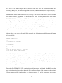
The following example illustrates the format of the input data file.
Synthetic data
1
1
1000.
12 2
1
0.
3 0
4.00
8.00
16.00
32.00
64.00
128.00
256.00
512.00
1024.00
2048.00
4096.00
8192.00
0.14219E+01
0.12220E+01
0.15243E+01
0.22128E+01
0.32212E+01
0.63994E+01
0.17812E+02
0.47480E+02
0.10998E+03
0.17153E+03
0.10288E+03
0.93610E+02
0.30574E+02
0.23876E+02
0.18217E+02
0.14607E+02
0.13006E+02
0.13824E+02
0.18135E+02
0.27415E+02
0.42078E+02
0.58351E+02
0.50792E+02
0.45630E+02
Lines 2 and 6 are used for comments. The first line defines a header text (max 30 characters). The
third line defines the source type (ISYS), response type (IMOD) and sounding type (IOPT). The
source is either a VMD (ISYS= 1) or a HMD (ISYS= 2 or 3). The response type is one of the nine
possibilities (IMOD= 1,2, …, or 9) defined in the Using the program chapter. The sounding type is
either frequency sounding (IOPT= 1) or geometric sounding (IOPT= 2). The 4.th line defines first
the loop spacing (m) or frequency (Hz) used in the frequency or geometric soundings, respectively.
The second parameter on the 4.th line defines the height (in meters) of the dipole-dipole system
from the surface of the earth. Note that the source and the receiver are always on the same height
level above or on the surface. The 5.th line defines the number of frequencies (NOF) and the
column indices (ICO1, ICO2 and ICO3) for the two response components (in this case apparent
resistivity and phase, since IMOD= 1) and weights used in the inversion. A data component can be
omitted if its column index is set to zero (ICO1= 0 or ICO2= 0). Likewise, weights are not read at
9
all if ICO3= 0 (as in the example above). The next NOF lines define the column-formatted data:
frequency (FREQ, Hz), the measured apparent resistivity (Ohmm) and the phase component (deg.).
The maximum amount of frequencies or loop spacings is 80 and the header text is used as a second
line in the response graph title. If the header text line is empty the default title in the
FDEMINV.DIS file is used instead. The frequencies (or loop spacings) must be either in an
ascending or in descending order. Note also that the data file can contain several data columns,
from which one or two are read for the interpretation. This means that the same data file can
contain, for example, measurements along a profile. Manual editing of the column indices is
(currently) required to choose the correct data column for the FDEMINV program. Data values
equal to zero are omitted and, thus, used for missing data values.
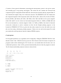
Although there is no need to edit model files manually, the following example illustrates the format
of the model files:
FDEMINV model file:
3
0.10000E+03
0.10000E+01
0.10000E+05
0.10000E+03
0.10000E+03
1
1
1
500.00
0.00
14
2. 4. 8. 16. 32. 64. 128. 256. 512.
1024. 2048. 4096. 8192. 16384.
Lines 1, 2 and 7 (in this case) are used for comments and can be left empty. The 3.rd line defines
the number of layers (NOL), the maximum amount of which is 6. Lines 4 and 5 define the
resistivity (RH, Ohmm) and the thickness (TH, m) of the two topmost layers and the 6.th line
defines the resistivity of the bottom layer. The 1.st line of the 2.nd paragraph defines the number of
frequencies (NOF). The frequency values are then provided at the end of the file. Note that the
frequencies can be given on multiple lines.
The results file (FDEMINV.OUT) contains the model parameters and depths, the RMS error, the
mean of the damping factors, the (damped) 95% confidence limits of the parameters, the original
(W) and normalized (S) singular values, the damping factors (T) and the parameter eigenvectors
10
(V-matrix). Some general information concerning the measurement system is also given (source
and sounding types, loop spacing and height). The results file also contains the measured and
computed response components and the difference between the measured and the computed data. It
also contains the weights if they were used in the inversion. The FDEMINV.OUT file contains also
the computed magnetic field components (H01, H02, Re,Im (H1), Re,Im (H2), Re,Im (H1/H01),
Re,Im (H2/H01) and Re,Im ((H1+H01)/ (H2+H02)). Here H01 and H02 are free-space magnetic
fields. H01 and H1 are the vertical (or horizontal) magnetic fields of a VMD (or HMD) H02 and
H2 are the horizontal (or vertical) magnetic fields of a VMD (or HMD). Note that for historical
reasons the #-character is used to comment out lines for the Gnuplot plotting program. At the
bottom the FDEMINV.OUT file are given the data values required to create the model curve and
the error bars using a third-party plotting program. If data were not read in the output file would
just contain the model parameters and the computed FDEM response.
Graph options:
Several graph parameters (see Appendix) can be changed by editing the FDEMINV.DIS file. Note
that the format of the *.DIS file must be preserved. If the format of the file becomes corrupted, the
program crashes while initializing the GUI. In this case, one should delete the file and a new one
with default parameter values will be generated automatically the next time the program is started.
The file format and default parameter values are shown below.
40
1
370
32
2
350
32
26
26
1
1
0.600 0.850 0.830
FDEM sounding
Test model
Response 1
Response 2
Frequency (Hz)
Loop spacing (m)
1.
2.
1.
2.
comp.
comp.
meas.
meas.
System and model description
Resist. (Ohmm)
Thickness (m)
Depth (m)
11
 The 1.st line defines five character heights. The first one is used for the main title and the graph
axis titles, the second height is used for the axis labels, the third height is used for the plot
legend text, the fourth height is used for the model description text, and the last height is used
for the axis labels in the model view.
 The 2.nd line contains integer valued parameters that define if the info text is shown or not, if
model view is drawn or not, if error bars are shown in the model view, in which corner the
legend is drawn and if widescreen mode is active or not.
 The 3.rd line defines parameters that define: the x- (horizontal) and y- (vertical) position of the
origin of the main graph (in pixels), the length of the x- and y-axis relative to the size of the total
width and height of the total plot area (eg. 0.5= 50 % of the width or height), which is equal to
29702100 pixels (landscape A4), and the screen aspect ratio for widescreen mode.
 The following lines define various text items of the graph (max. 40 characters).
 Two main titles of the response graph.
 Three axis names of the graph. When both data channels are plotted the x-axis title shows
both axis names (Response 1 + Response 2).
 Four legend texts (computed and measured).
 One title of the model description text
 Two column headers of the model parameters
 One additional axis title for vertical axis of the model view
Note that to mimic depth sounding the response lies on the horizontal x-axis and the vertical y-axis
is the parametric (frequency or loop spacing) axis. Note also that by default the graph does not
contain the actual names and units of all the nine different the response types. Instead, generic
names (e.g., Resp. 1 and Resp. 2) are provided and the response type is shown in the description
text in the top right corner of the graph page defines. Manual editing of the FDEMINV.DIS file is
required, if printed graphs are going to be prepared for presentation purposes.
Note that the DISLIN graphics allows the use of special characters in graph texts. The instructions
are placed between "{" and "}" characters. For example, the text "Resistivity ({M2}W{M1}m)"
will produce "Resistivity (m)". See the DISLIN documentation for further information.
12
Additional information
Originally, I made the FDEMINV program at the University of Oulu in December 2001, when I
worked as a researcher funded by a grant from Outokumpu Foundation addressed to Prof. SvenErik Hjelt. Afterwards I’ve updated the program every now and then.
The forward computation is based on the well-known solution for magnetic dipole sources above
1-D layered earth (e.g., Keller and Friscknecht, 1967). The convolution algorithm and the filter
coefficients used to compute the Hankel transforms are based on the work of N.B. Christensen,
(Geoph. Prospecting, 1990, vol 38, pp. 545-568). The inversion method, which is based on the
singular value decomposition and adaptive damping method, is described in my PhD thesis (M.
Pirttijärvi, 2003. Acta Univ. Oul., A 403).
The FDEMINV program is written in Fortran 90 and compiled with Intel Visual Fortran 11.1. The
graphical user interface is based on the DISLIN graphics library (version 10.2) by Helmut Michels.
The program distribution includes the DISDLL.DLL that is required for the 32-bit GUI. Since the
DISLIN graphics library is independent form the operating system the FDEMINV program could
be compiled on other operating systems (Mac OSX, Linux) without any modifications. At the
moment, however, the source code is not made available and I do not intend to provide any support
for the program. If you find the computed results erroneous or if you have suggestions for
improvements, please, inform me.
Note that the FDEMINV program has not been tested thoroughly and that its usability in data
interpretation is quite modest. For example, currently the program does not use proper data
weighting, although it always works with the 10-base logarithms of both the data and the
parameters. Interpretation of frequency domain soundings are going to be implemented in future
version of Jointem, software for joint interpretation of TEM, VES, VLF-R and AMT/MT
soundings. For more information about the current status of Jointem and other software, please,
visit my web page at https://wiki.oulu.fi/display/[email protected] .
13
Terms of use and disclaimer:
You can use the FDEMINV program free of charge. If you find the program useful, please, send
me a postcard.The program is provided as is. The author (MP) and the University of Oulu disclaim
all warranties, expressed or implied, with regard to this software. In no event shall the author or the
University of Oulu be liable for any indirect or consequential damages or any damages whatsoever
resulting from loss of use, data or profits, arising out of or in connection with the use or
performance of this software.
Contact information:
Markku Pirttijärvi, PhD
Department of Physics
Tel: +358-8-5531409
FIN-90014 University of Oulu
URL: https://wiki.oulu.fi/display/[email protected]
Finland
E-mail: markku.pirttijarv(at)oulu.fi
14
Appendix:
15