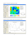
1
GRABLOX
Gravity interpretation and modeling software based on a 3-D block model
Version 1.6b
User's guide
Markku Pirttijärvi
9/2008
University of Oulu
Department of Physical Sciences
Division of Geophysics
Table of contents
Table of contents ................................................................................................................... 2 1. Introduction ....................................................................................................................... 3 2. Installing the program........................................................................................................ 5 3. Getting started ................................................................................................................... 6 4. The GRABLOX user interface .......................................................................................... 7 5.1 File menu ..................................................................................................................... 7 4.2 Gravity menu ............................................................................................................... 8 4.3 Edit menu................................................................................................................... 11 4.4 Exit menu................................................................................................................... 13 4.5 Left control pane ........................................................................................................ 13 4.6 Right control pane ..................................................................................................... 18 5. Inversion methods ........................................................................................................... 22 5.1 Regional field ............................................................................................................ 22 5.2 Fix/free status ............................................................................................................ 24 5.3 Depth weighting ........................................................................................................ 24 5.4 Normal SVD based inversion .................................................................................... 25 5.4.1 Additional constraining and bulky inversion ..................................................... 26 5.5 Occam inversion ........................................................................................................ 27 5.5.1 Occam d, Occam h, and Occam d+h methods.................................................... 28 5.5.2 Lagrange multiplier ............................................................................................ 29 5.5.3 Parameter roughness ........................................................................................... 30 5.6 Inversion parameters.................................................................................................. 30 5.7 Computation times ..................................................................................................... 32 6. Guidelines for gravity inversion ...................................................................................... 33 6.1 Precautions................................................................................................................. 33 6.2 Data preparation ........................................................................................................ 34 6.3 Preliminary operations............................................................................................... 35 6.4 Initial model ............................................................................................................... 35 6.5 A priori data ............................................................................................................... 38 6.6 Gravity inversion ....................................................................................................... 39 6.6.1 Base anomaly inversion ...................................................................................... 40 6.6.2 3-D density inversion ......................................................................................... 42 6.6.3 Two-layer height inversion................................................................................. 44 6.7 Post-processing .......................................................................................................... 46 7. File formats ...................................................................................................................... 48 7.1 Model files ................................................................................................................. 48 7.2 Data files .................................................................................................................... 51 7.3 Output files ................................................................................................................ 52 7.4 Graph options ............................................................................................................ 53 8. Additional information .................................................................................................... 55 9. References ....................................................................................................................... 56 10. Terms of use and disclaimer .......................................................................................... 57 11. Contact information ....................................................................................................... 57 Appendices
Keywords: geophysics; gravity; 3-D models; modelling; inversion; Occam.
2
1. Introduction
Gravity measurements provide an indirect method to study the internal geological structure of
the Earth. The measured gravity field is caused mainly by the gravitational attraction of
Earth's mass, the ellipsoidal shape of the Earth and the centrifugal force due to Earth's rotation
around its axis. These latitude dependent features of Earth's gravity field can be modelled
using the international gravity formula (IGF). Because of the atom weight of the elements, the
element composition and structure of minerals and the mineral composition and structure of
rocks and soil the gravity field is not uniform on the surface of the Earth. The governing
petrophysical parameter is the density, ρ [kg/m3], defined as the mass (weight) per volume.
Together with topography (elevation) changes the density variations inside the Earth give rise
to gravity anomalies. In large scale studies the amplitude of the gravity anomalies can be
several tens on milligals (1 mgal = 10-5 m/s2). In small-scale studies the anomalies are less
than one milligal. Thus, accurate determination of gravity and elevation as well as precise
data correction and reduction are needed.
Absolute gravity measurements are made to determine Earth's (vertical) gravitational
acceleration, g (gn ≈ 9.80665 m/s2) directly. Relative measurements are made in applied
geophysics to determine the difference Δg between two or more measurement sites. Known
reference points can be used to tie the relative gravity measurements into absolute values.
However, absolute gravity values are rarely used in gravity modeling. Instead, the
measurements are represented as Bouguer-anomaly, where the data are reduced to the sea
level (reference ellipsoid used in IGF) by free-air and Bouguer corrections. Sometimes
topographic and isostatic corrections are made to gravity data also. For more information of
gravity method, please, see Blakely (1995) or any text book of applied geophysics.
The objective the gravity interpretation of gravity measurements made on Earth’s surface is to
determine the density contrast and/or the shape and dimensions of the density variations.
Gravity interpretation is an inverse problem. Unfortunately, gravity data cannot be interpreted
uniquely. The objective is to use density model and to use inversion to construct such a
density distribution that would explain the measurements. Therefore, special care must be
taken when assessing the geological validity of the geophysical interpretation model.
3
The GRABLOX program computes the synthetic gravity anomaly of a 3-D block model.
Figure 1 illustrates the model – a large rectangular super block, which is divided into smaller
brick-like volume elements. Each minor block is assigned an individual, constant density
value. For more information about 3-D block models, please, see the documentation of the
BLOXER program, which can be used to visualize and to edit the 3-D block models.
Figure 1. Block model of size dX × dY × dZ (distance units) divided into N = nx × ny × nz
minor blocks of size dx × dy × dz (distance units). The model is aligned with the
(geographical) coordinate system.
The GRABLOX program can be used both for forward and inverse modeling (inversion). The
inversion method optimizes either the density or the height of the individual blocks so that the
difference between the measured and the computed gravity data gets minimized. The height
inversion allows interpretation of the thickness variations of the overburden layer (depth to
the basement) using constant density contrast. The distribution of the resulting density or
thickness variations inside the block model can then be used in geological interpretation.
GRABLOX can be used for both (large-scale) regional studies and (small-scale) local studies.
Separate BLOXER program can be used for model editing and visualization.
The optimization method is based on linearized inversion. The original inversion method uses
singular value decomposition (SVD) with adaptive damping. The alternative inversion
method utilizes Occam's principle where the roughness of the model is minimized together
with data misfit. The parameters of a base anomaly represented by a polynomial of a second
degree can be optimized also. Density and the interface position of the blocks can be fixed
(weighted) based on a priori information (e.g., petrophysical or drill-hole data).
4
2. Installing the program
The GRABLOX program requires a PC with Microsoft Windows 98/XP/Vista operating
system and a graphics display with a screen resolution of at least 1024×768 pixels. Presently
the program has not been tested on Windows Vista. In forward modeling memory
requirements and processor speed are usually not critical factors, because the program uses
dynamic memory allocation and the forward computation is quite fast. However, computation
of models with hundreds of thousands of elements may take several hours even on modern
PC's. Moreover, inversion of block models with more than ten thousand elements is not
practical because of the increased computation time.
The program has a simple graphical user interface (GUI) that can be used to modify the
parameter values, to handle file input and output, and to visualize the gravity data and the
model. The user interface is based on the DISLIN graphics library.
The program requires two files:
GRABLOX.EXE
DISDLL.DLL
The
distribution
the executable file,
dynamic link library for the DISLIN graphics.
file
(GRABLOX.ZIP)
also
contains
a
short
description
file
(_README.TXT), a user's manual (GRABLOX_MANU.PDF), and example data (*.DAT)
and model files (*.INP & *.BLX). To install the program simply uncompress (with
Pkzip/Winzip) the distribution files into a new folder. To be able to start the program from a
shortcut that locates in a different directory, the DISDLL.DLL file should be copied or moved
into the system folder. Alternatively one can modify the PATH environment variable. When
running the program over network one should map the network drive (e.g., Explorer/Tools/
Map network drive…) and provide it with a logical drive letter.
The included GRABLOC.EXE program is a non-GUI version that can be used to perform the
forward solution alone. Please, note that GRABLOC always reads its input from the
GRABLOC.INP and GRABLOC.BLX files.
5
3. Getting started
On startup the program shows a standard file selection dialog, which is used to provide the
name of the input model file (*.INP). If the user cancels the file selection operation the
GRABLOX.INP file will be used. If this file does not exist default parameters are used and
the file will be created automatically. The parameters of individual blocks are read from a
separate *.BLX file. Before the user interface is built up, the program reads graph parameters
from the GRABLOX.DIS file. If this file does not exist default parameters are used and the
file is created automatically.
The program runs in two windows: the console window (command shell) and the graphical
user interface (GUI) window. The console window is used to provide runtime information
about the current status of the program.
After the initial model and the system parameters have been defined the program builds up
the user interface (see the Appendices). At this point the graph area will be blank because
forward computation has not been made and measured data have not been read in. However,
the model can be visualized using the Layers and Sections push buttons (Appendices A and
B). Repetitive use of Layers and Sections push buttons will show successive layers or
sections. The Crossing dir button swaps between (West-East directed) X-section and (SouthNorth directed) Y-section views. The <-/-> button is used to reverse the direction of layer or
section swapping.
The Compute push button on top of the right control pane of the application window is used
to perform a forward computation. The Contours button is used to plot the data as a 2-D
colored contour map along with a 3-D view of the model and a short description on some
parameters (Appendix C). The Profiles push button can be used to display a single profile
across the model area and the Crossing dir button swaps between SN and WE directed
profiles (Appendix D). Model and system parameters can be changed using the text fields on
the left control pane. The Update button must be pressed to validate the changes. The
computational options can be changed using the items in the Gravity menu. Before measured
data have not been read in most of the controls on the right control pane are inactive. To learn
more about data interpretation, please, refer to chapters 5 and 6.
6
4. The GRABLOX user interface
5.1 File menu
Open model
open an existing model file.
Read data
read in data for interpretation and comparison.
Read regional
read in regional data (stationary gravity field).
Save model
save the model into a file.
Save data
save the data (computed & measured) into a file.
Save results
save the results (description & data) into a file.
Read disp
read in new graph parameters from a *.DIS file.
Save graph as PS
save the graph in Adobe's Postscript format.
Save graph as EPS
save the graph in Adobe's Encapsulated Postscript format.
Save graph as PDF
save the graph in Adobe's (Acrobat) PDF format.
Save graph as WMF
save the graph in Windows metafile format.
Save graph as GIF
save the graph in GIF (graphics interchange format) format.
These menu options will bring up a standard (Windows) file selection dialog that can be used
to provide the name for the file for open/save operation. Model files (*.INP) files are saved in
text format and the parameters of the minor blocks are stored in a separate *.BLX file, with
the same prefix name as the *.INP file. When saving the results, GRABLOX stores text
information into an *.OUT file, the data into a *.GBM file, and makes a header file (*.HEG)
that describes the format of the data file. Measured data are read form a column formatted
data (*.DAT) files, which are in (ASCII/ISO8859) text format. The Save data entry generates
a *.DAT file in the same format. See chapter 8 for more information about the file formats.
GRABLOX does not support direct printing. The graphs are saved in files that can be viewed
and printed using a suitable third party programs (e.g., Ghostview, Paint Shop Pro, Adobe
Acrobat Reader, MS Word, etc.). All graphs are saved in landscape A4 size as they appear on
the screen. The GIF option is the only bitmap format (size 2970×2100 pixels). The EPS file
does not include preview bitmap.
7
4.2 Gravity menu
Comp → Meas
replace the measured data with the computed response.
Comp → Regi
replace the regional field with the computed response.
Subtract regional
remove the regional field from measured data.
Remove measured
remove all information about measured data.
Compute default
build up a default model based on measured data coordinates.
Scale unit
define dimensions in meters, kilometers, feet or miles.
Gravity field
swap between total field and anomalous response.
Computation method
choose the computation method: blocks, points, vert.derivative.
Background method
set the background: given value, layer mean, whole model mean.
Depth weighting
disable/enable partially or enable totally.
Enable bulkiness
enable/disable rounding of parameter values in inversion.
Enable roughness
enable/disable use of the roughness parameter in inversion.
Enable inversion
enable/disable the inversion.
• The Comp→Meas and Remove measured items are useful when using the program for
testing and educational purposes.
• The Comp→Regi item can be used to define a regional field using the current model.
Alternatively one can use the Read Reg. Field menu item to read in regional field data.
• The Subtract regional item can be used to remove the current regional field (if it has been
read in or defined otherwise) and/or base anomaly level from the measured data. Removing
the regional trend can reveal small features in the data. By saving the new data into a file
(Save data in File menu) one can define a new dataset where the regional gravity effect has
been removed.
• The Compute default item is useful after new measured data has been read in, because it
automatically gives the super block some reasonable coordinates inside the data area. If the
data appears to be regularly gridded GRABLOX also discretizes the model so that the
blocks are put below each data points (z coordinates also). Note that 2-D surface data and
profile data are handled differently. When dealing with irregular data the user should
provide an appropriate position, size and discretization for the super block manually.
• When GRABLOX reads in data it does not know the units of the coordinates and distances.
The Scale unit item defines the actual volume of the block model, and hence, the correct
8
gravity values. Therefore, the user should supply correct scale (meters, kilometers, or
miles) before continuing with the modeling or interpretation. The information about the
units will be stored in the model file and used in output files.
• The computed gravity field (gc) is a sum of the gravity effect of the model blocks (gm),
base anomaly (gb) and regional field (gr)
gc = gm + gb + gr
If regional field (gr) has been defined the Gravity field item can be used to change include
(total field) or exclude (anomalous field) the regional field from it. The base anomaly (gb)
is always added to the computed response.
• The Computation method item defines the three modes of the gravity computation:
1. The gravity effect is computed using actual prism-like minor blocks.
2. The gravity effect is computed using point sources, that is, spherical sources the
volumes of which are equal to the volumes of the actual blocks. This method is less
accurate than the block-model approach.
3. The vertical gradient of the gravity effect is computed using prism-like minor blocks.
Note that point sources should be used only if equal sized blocks are used and the model is
densely discretized (with millions of elements). The point source approach is about 18 times
faster than block model computation, but because the accuracy of this method is difficult to
assess, it should be used only to provide coarse first order approximation to the gravity effect.
When using point sources the model and computation grid should be made regular so that the
blocks are located directly below the computation points.
• The Background method item is used to choose between three modes for the definition of
background density:
1. Normally the background density value is defined by the Bg dens text field on the left
control pane. In this case the background density value is subtracted from the density
values of each minor block. Thus, if the density of the block is equal to the background
value it has no effect in the computed gravity anomaly.
9
2. In large-scale crustal studies the background density value is defined separately for each
depth using the mean density of the blocks of each layer. The mean density is then
subtracted from the density of each minor block. This method is useful in large-scale
crustal models where the density is assumed to increase downwards.
3. Sometimes it may be useful to define the background density value as the mean value of
all the minor blocks of the model. Thus, the mean density of the whole block model is
subtracted from the density values of each minor block. This method allows a simple
way to define floating background value. If the density increases downwards this
method is not as good as the second one.
The purpose of the background density value is to remove (or reduce) the effect of the four
sides of the super block when the model contains absolute density values. If background
density is not used (or the contrast is large) the super block shows up as a single source,
which creates a very strong gravity anomaly, and the effects of its internal density variations
will not be visible at all.
The depth weighting is used in gravity inversion to give additional importance to the deeper
parts of the model. As a consequence, the inversion will place the mass distributions at their
"correct" depth instead of placing them near the surface as would happen without depth
weighting. The meaning of the three modes of depth weighting (ignore, relaxed and fixed) is
discussed in chapter 5.3.
Usually the background density can be set to zero and the inversion will resolve the residual
density. When absolute density values, for example, from petrophysical samples are available
the given background value can be set equal to the mean of the sample values. Usually,
however, the background density is set equal to the density used in Bouguer and topographic
corrections (e.g., 2670 kg/m3).
The last three items in the Gravity menu are related to inversion:
• The Bulkiness option restricts the density values so that they are rounded to nearest
classified value. See chapter 5.4 for more information.
• The Roughness option allows using discontinuity information in the Occam inversion. The
discontinuity information is stored in to the model file as a second parameter with the help
10
of the BLOXER program. If the file does not contain roughness values, this menu item will
be inactive. See chapter 5.5 for more information
• The Enable inversion item defines whether or not the sensitivity matrix (Jacobian) will be
computed automatically during forward computation. For example, when Comp→Meas
item is used to set computed (synthetic) data to measured data, inversion is not enabled by
default and this menu item must to be used to activate inversion and related controls and
menus. Note that when actual measured data is read in, the inversion is enabled by default.
However, if the model is very large the program may be unable to allocate memory for the
Jacobian. In this case GRABLOX disables the inversion and computes only the forward
solution. Thus, menu item can be used to enable the inversion after new model with
smaller amount of elements has been defined.
4.3 Edit menu
Block type
swap between equal-sized and increasing height block modes.
Min/Max values
redefine the min & max parameter value on the color scale.
Layer-wise fix/free
set the fix/free/hidden status of the blocks per each layer.
Layer-wise reset
set the density value of the blocks per each layer.
Add margins
adds marginal areas around the super block (layer inversion).
Del margins
removes the marginal areas around the super block.
Labels
hides or defines the information shown as parameter labels.
Show/Hide grid
show or hide the block outlines in 2-D graphs.
Contour/Image
show the 2-D gravity data as contour maps or image maps.
Show/Hide regional show or hide regional field or base anomaly from graphs.
Color scale
change the color scale used in the graphs.
• Although the xyz dimensions of the blocks can vary, all blocks have equal size by default.
In the alternative block type (Block type 2) the height of the blocks will systematically
increase downwards by the height value of the topmost layer of blocks (e.g. 0.5, 1, 1.5, 2,
2.5 km). The alternative block sizing thus reduces the resolution at the bottom but helps
decreasing the total number of blocks.
• The Min/Max values item not only changes the limiting density values on the color scale
(below the layers or sections view) but it also determines the absolute minimum and
11
maximum density values used in the inversion. These values, in turn, determine the
maximum parameter steps in SVD based inversion. The new values are given as a text
string into a dialog appearing on the screen. The input dialog does not contain a cancel
button. Therefore, to cancel the operation one should close the dialog from the icon (cross)
at the top-right corner or pass an empty input line. The same applies to some other tasks
involving the input dialog as described below.
• Layer-wise fix/free option allows setting the fix/free (weights) and hidden status of the
blocks for each layer manually. Weights are integer values between -101 and 100. Value
equal to zero will fix the layer during inversion. Value equal to 1 or 100 gives the whole
layer a fully free status. Value between 2 and 99 gives decreasing weight so that 2 is
almost fixed and 99 is almost free. Value equal to -1 (or less than zero) hides the layer
totally. The new values are given as a text string into a dialog appearing on the screen. See
chapter 5.2 for more information about the fix/free status.
• Layer-wise reset option allows setting the density value of the blocks for each layer
manually. The new values are given as a text string into a dialog appearing on the screen.
• The Labels and Show/Hide grid items can be used to clarify the contour/image maps as
well as the layer and section graphs. The Labels option either removes the labels totally, or
shows either the density, block height, block depth, fix/free (weights) satus, or roughness
values (if available).
• The Show regional item allows visualizing the regional trend (read in regional data and the
base anomaly) in the computed response. The Hide regional item is useful when the
difference between the measured (or computed) data and the regional field (or base
anomaly) is so large that the fit between measured and computed data is difficult to see in
profile graphs.
• Margins are important when interpreting gravity data using a two-layer model with
constant density contrast. The margins extend the edge-effect of the topmost layer away
from the computation area. The new values are given as a text string into a dialog
appearing on the screen.
• The preparation of contour plots can be time consuming if there are lots of data points.
Moreover, the interpolation can easily create artifacts that arise from irregularly spaced
data points. Therefore, the data can be plotted also as an image map.
12
• The Color scale item can be used to choose between normal rainbow scale, inverted
rainbow scale, normal grayscale, inverted grayscale and a special (seismic/temperature)
red-white scale.
4.4 Exit menu
The Widescreen item is used to restart the graphical user interface with a window size and
shape that suits either the conventional 4:3 display or a widescreen and laptop display. The
Exit item is used to confirm the exit operation. On exit the user is given an opportunity to save
the current model and the results, provided that exiting is made without an error condition. On
exit, the program first asks the name for the model file (*.INP & *.BLX) and then the
filename for the results (*.OUT, *.HEG & *.GBM). If the user cancels the save operation
after choosing to save the model or results, the default filenames GRABLOX.* will be used.
Errors that are encountered before the GUI starts up are reported in the GRABLOX.ERR file.
When operating in GUI mode, run-time errors arising from illegal parameter values are
displayed on the screen. Some errors, however, cannot be traced and given an explanation.
The most typical problem is perhaps a corrupted GRABLOX.DIS file that prevents the
program to start up properly. This problem can be circumvented simply by deleting the
existing *.DIS file. A missing or incorrectly named *.BLX file can also cause troubles.
Please, note that most messages that appear on the console window are stored also into a log
file GRABLOX.LOG. This file is written over when the program is restarted so one may need
to rename to save it.
4.5 Left control pane
The Update button is used (and must be used) to validate the changes made to the model
parameters. After pressing the Update button, the values of the various text fields defining the
position, size, and discretization of the block model are read in and checked for erroneous
values, and the old values are replaced with the new ones. Be warned that currently the use of
the Update button always invalidates previous results and new computation is needed.
The list widget below the Update button defines how the block parameters will be affected
when the Update button is pressed.
13
1. The Shift only mode updates only the xyz position of the whole block model. The size
and the discretization of the super block cannot be changed in Shift only mode. This is
the default mode and it is purpose is to protect the model from accidental changes.
2. The Ignore mode allows easy redefining of the size and discretization of the super
block. However, the Ignore mode ignores the relationship between the position and the
density of the blocks. The density of the blocks remain the same but they will move
around inside the model if the discretization changes.
3. The Preserve mode uses 3-D nearest neighbor interpolation method to determine new
parameter values when the block is resized, rediscretized, or repositioned. For example,
if the position of the super block is shifted, the position of an anomalous density
contrast will remain at the same xyz position, but its relative position inside the super
block will change. Note that 3-D interpolation of densely discretized and large models
can be very time consuming.
The following text fields define the position, size and discretization of the super block:
1. X position (easting) of the SW (bottom-left) corner of the super block.
2. Y position (northing) of the SW (bottom-left) corner of the super block.
3. Z position (depth to the top) of the super block.
4. X size of the super block (in EW direction).
5. Y size of the super block (in NS direction).
6. Z size of the super block (in vertical direction).
7. X discretization (number of blocks) in EW-direction.
8. Y discretization (number of blocks) in NS-direction.
9. Z discretization (number of blocks) in vertical direction.
In GRABLOX the true dimensions of the block model (and the computation grid) are defined
using the Gravity-Scale unit menu item. The given rectangular coordinates do not need to be
actual geographic map coordinates. To be able to better model geological strike directions, for
example, the data and the model can be provided with rotated coordinates. However, the
coordinate transforms need to be made outside GRABLOX, because it does not have the
functionality to rotate the model or data.
14
The next two text fields define two density parameters:
1. Bg dens defines the value of user defined background density (g/cm3).
2. Param defines the default density value used to reset the model (g/cm3)
The Reset param button is used to reset the density value of the whole super block to the
value defined by the Param text field above the Reset param button. Note that fixed blocks
are protected and will not be affected.
The density is defined in units [g/cm3] (grams per cubic centimeter). Use the BLOXER
program transform to transform the units (g/cm3 ↔ kg/m3) if needed.
The gravity anomalies (computed, measured, regional and base) are defined in units
[mGal] (milliGals), where 1 mGal = 10-5 m/s2 (note 10-6 m/s2 = 0.1 mGal).
The gravity anomaly is always computed using a density contrast Δρ = ρi - ρ0, i.e., the
difference between the density of the blocks (ρi ) and the background density (ρ0). The
method used to define the background density is chosen using the Gravity-Background
method menu item. When Given value mode is active, the value of background density
provided in Bg dens field will be subtracted from the density values of each minor block.
Note that the density values can be either absolute (e.g., ranging between 2000 and 3600
kg/m3) or relative (ranging between -600 and +1000 kg/m3) depending on the value of
background density.
When performing forward computations the computation points are usually defined on a
regular grid, which is defined by the seven text fields below the Reset param button:
1. The spatial x step between points of the computation grid.
2. The spatial y step between points of the computation grid.
3. The x coordinate (easting) of the grid start position.
4. The y coordinate (northing) of the grid start position.
5. The x coordinate (easting) of the grid end position.
6. The y coordinate (northing) of the grid end position.
7. The z level (height or elevation) of the computation grid.
15
If either the x or y step is equal to zero or the width of the computation grid is zero either in x
or y direction the computations are made along a single profile extending from (x1,y1,z) to
(x2, y2,z). The non-zero x or y step is used as a distance between the computation points.
Naturally, in this case only profile plots can be shown (no contour or image maps).
When measured data are read in they are assumed to be irregularly spaced. The computations
are always made at the actual measurement locations (x,y,z). Therefore the start and end
positions of the computation grid are inactive when data has been read in. The x and y steps,
however, are used to define grid spacing in contour and image maps. When irregularly spaced
data has been read in, the x and y steps should be set manually to reduce possible artifacts in
the contouring.
The z coordinates (elevation or topography) of the measured data are used if they are given
AND the Z-level parameter is equal to the top of the super block (Z-posit.). Otherwise,
response is computed at a constant elevation value given by the Z-level text field. This method
allows fast inspection of the effect of height in the gravity computations.
The remaining eight text fields are used to define a computational base anomaly using a
second degree polynomial of a form:
gb(x,y) = A + B(x-x0) + C(y-y0) + D(x-x0)2 + E(y-y0)2 +F(x-x0)×(y-y0),
where x0 and y0 are offset coordinates that define the shifted origin. By default the origin (x0,
y0) is located at the middle of the super block. Because the amplitude changes of gravity
anomalies are small compared to distances the coefficients C and D are scaled (multiplied) by
1000 and E and F are scaled by 105. The base anomaly is always added to the computed
gravity anomaly even if external regional field has been read in. However, the base anomaly
cannot be visualized as a contour or profile plot without the regional field (see also
Show/Hide regional menu item).
The Update base button at the bottom of the left control pane is used to set and to update the
changes made to the base level immediately without the need to compute the response of the
block model.
16
17
4.6 Right control pane
The Compute button is used to perform the forward computation using the current values of
the model and system parameters.
The Optimize push button is used to start the inversion. Note that depending on the total
number of minor blocks and the amount of computation points, the inversion can take a
considerable amount of time.
The list widget below the Optimize button defines the six primary inversion types:
1. Base: the values of the parameters of the base anomaly.
2. Density: the density of the blocks using SVD based inversion.
3. Occam d: the density of the blocks using Occam's method, where both the data misfit
(difference between the measured data and the computed response) and the model
roughness are minimized.
4. Heights: the height of the blocks using SVD based inversion. The height optimization
affects the depth extent, i.e, the depth to the bottom of the blocks. The bottom layer is
never optimized.
5. Occam h: the height of all the blocks using Occam's method.
6. Occam h+d: the height of the blocks together with the mean density of each layer of the
block model.
The second list widget defines additional constraining method in Density, Occam d and
Height inversion options.
1. Normal method does not give any additional constraints for the parameter values.
2. Smooth vertical mode additionally constrains only the vertical parameter variation. The
resulting model will therefore have more rough parameter variation horizontally.
3. Smooth horizontal mode constrains the horizontal parameter variation. The resulting
model should therefore have more rough density (or height) variation in vertically.
4. Smooth 3-D mode tries to generate a smooth model in all three directions.
18
The SVD based Density and Height inversion are so-called unconstrained inversion methods,
where fixed blocks have no effect on the inversion of surrounding blocks. The
abovementioned options provide a poor-man's constraining by limiting the new parameter
value based on the mean of the neighboring blocks. The allowed parameter variation is
defined by the Step % text field discussed below. The Height inversion utilizes only
horizontal smoothing or no smoothing at all. In Occam d optimization the abovementioned
options redefine the method used to compute the local roughness.
The third list widget defines the parameters of the base anomaly that are going to be
optimized when Base optimization is made. Note that in Occam d, Occam h and Occam h+d
inversions the linear trend (A+Bx+Cy) of the base anomaly can be optimized together with
block densities or heights. Because base anomaly can be used to define long wavelength
variations in the data, one should remember to exclude the base response (select none) if one
does not want it to be optimized. Note that in practice combined inversion of base anomaly
and block parameters requires that some additional a priori information is available and some
parameters have been fixed.
The following five text fields define few inversion parameters.
1. The Iters field defines the number of iterations made during one inversion run.
2. The Thres % value defines the strength of damping in Base, Density and Height
inversions. Normally the threshold should be at the level of the smallest singular values
that are still "informative". The smaller the threshold value is the weaker is the
damping. Note that the value given for the threshold is divided by 100 so the default
value 0.01 (%) is actually 0.0001.
3. The Step % value defines the parameter stepping used in bulky inversion and the
maximum parameter change in the additional constraining methods. It also defines the
parameter step used to obtain the partial derivatives (forward difference) for the
Jacobian when optimizing block heights. Note that the value given for the step is
divided by 100, so the default value 2.5 (%) is actually 0,025.
4. The F-option parameter is used to provide additional (real valued) numerical value to
the inversion. Its role depends on the selected inversion type. In SVD based inversion it
determines the maximum step controlling the convergence. In Occam inversion it is
used as a Lagrange multiplier controlling model vs. data smoothness.
19
5. The I-option parameter is used to provide additional (integer valued) numerical value to
the inversion. In Occam inversion it is used to control the rigidity of fixed blocks and in
base inversion it is used to shift the fit towards the bottom of the gravity anomaly.
See chapter 6 for detailed information about the different inversion options discussed above.
The next two text fields are used in basic forward modeling and visualization.
1. The Trim value defines a limiting residual density value. If the absolute value of the
difference between the background density value (which depends on the GravityBackground method menu item) and the density of a minor block is less than the
trimming value then the effect of that block is not computed at all. This option concerns
the forward computation only.
2. The Layr/Sexn text field defines the index number of the current layer or section when
the model is being visualized (see the meaning of the buttons below). It is possible to
jump from one layer or section into another by first providing the new index number
and then pressing the corresponding Layers or Sections button.
The following six buttons are used to change the contents of the graph area.
1. The Contours button is used to show a 2-D color-filled contour plot or an image plot of
the gravity data. If measured data was read in, repetitive use of the Contours button will
swap the view between the computed, measured, and regional/base response data, and
the data error (difference between measured and computed data).
2. The Layers button is used to show the density values across a horizontal layer.
3. The Sections button is used to show the density values across a vertical cross-section.
4. The Profiles button is used to show the curves of computed, regional/base anomaly, and
measured data.
5. The Crossing dir. button is used to change the direction of the sections views and data
profiles between (vertical) SN and (horizontal) WE directions.
6. The <-/-> button is used to change the direction towards which the contours, layers,
sections and profiles are being rotated when pressed multiple times. This button affects
also the rotation direction of some other tasks, such as the selection of color scale.
20
Note that when the Layers, Sections, and Profiles buttons are pressed multiple times (rotates)
the current layer, section or profile changes to the next (or previous) one. At the last (or first)
layer, section or profile the view jumps to the first (or last) one. One can jump directly into a
desired layer or section by first providing the index number on the Layer/Sexn text field and
then pressing the corresponding push button.
Note that the profile data does not display the actual data, which are assumed irregularly
spaced. Instead it shows the interpolated data, where the "number of profiles" and the "point
step" are based on the interpolation density, i.e, the X-stp and Y-stp values in the left control
pane. If the data are highly irregular, the contouring algorithm produces bad artifacts. In such
a case, the Edit-Contour/Image menu item should be used to change the data representation
from a contour map to an image map. Alternatively the data should be mapped on a regular
grid using some third party interpolation software (e.g. Golden Software Surfer, or Geosoft
Oasis Montaj).
GRABLOX can be used also for 2.5-D interpretation of single profile data. In this case the
data are always read in so that the data profile is located along the x-axis. Consequently, the
model needs to be discretized along the x direction only (y discretization can be equal to one).
Moreover, contour and image maps and Y-sections cannot be displayed and the profile
representation shows the actual data points along a single profile. Note, however, that 2.5-D
inversion has not been tested thoroughly in GRABLOX version 1.6.
Normally, the vertical depth axis is plotted in 1:1 scale with horizontal axes in X and Ysection views. The Vert. scale slide control can be used to stretch or squeeze the depth axis. It
is useful if the height of the model is considerably smaller than its horizontal dimensions. The
other three slide controls (Horiz. rotation, Vert. rotation and Rel. distance) are used to change
the view point of the 3-D model views.
21
5. Inversion methods
This chapter discusses the inversion methods and the various terms used in GRABLOX. The
six different inversion methods used in GRABLOX are:
Base
normal SVD based optimization of the base response (level and gradients)
Density
normal SVD based optimization of the density
Height
normal SVD based optimization of the block height
Occam d
constrained Occam inversion of the density
Occam h
constrained Occam inversion of the block height
Occam h+d
combined Occam inversion of height and the mean layer density.
In density inversion the density values are limited by the minimum (Min) and maximum
(Max) values of the color scale shown below the Layer and Section graphs. The limit values
can be changed using the Edit-Min/Max values menu item.
In height inversion the block height values are limited by the height of the block itself and the
one beneath it, because a change in the height (depth extent) of one block affects the height
(depth to the top) of the block below it even if it is fixed. The height of the blocks of the
bottom layer cannot be optimized. The height of a block can never be less or equal to zero.
5.1 Regional field
Because the true density variations of the entire Earth cannot be modeled, we cannot compute
absolute gravity values. Instead we define the measurements as relative gravity anomalies
(e.g. Bouguer anomaly). The measured gravity anomaly, however, is caused by mass
distributions both near to and far away from the study area. The purpose of the regional field
is to subtract the gravity effect of all those masses that are located around and below the study
volume so that the inversion would need to find out the gravity effect of only those masses
that are located inside the volume of the model. Although the regional field can be defined
almost arbitrarily, the important thing is that it should not contain any gravity effects that
might be explained by density variations within the volume of the local model.
In GRABLOX the regional field can be defined in three different ways:
22
1. User-defined base response (base anomaly defined by a second degree polynomial),
2. Regional field is read together with the measured data (Read data), or
3. Regional field is read from a separate file (Read regional).
Best results are obtained if the regional field can be interpreted separately using gravity data
that extends (horizontally and vertically) 2−5 times farther than the actual interpretation
model of the study area. The block size of the regional model can be 2−10 times larger than
what will be used in local modelling. The important thing is to set the discretization of the
local and regional models so that the block boundaries (sides and bottom) of the local model
will fit the discretization of the regional model. Once the regional-scale inversion has been
made and an acceptable model has been found, the volume of the local study area is removed
(hidden) from the regional model (with BLOXER) and the regional, large-scale gravity
anomalies of the surroundings are computed at the data locations of the local study area and
saved into file.
Alternatively, surface fitting or low-pass filtering (Surfer, Geosoft) can be used to define the
regional trend of the gravity anomaly. These methods, however, are somewhat vague, because
they do not take into account the real physics and the depth extent of the targets. Therefore,
more advanced Fourier transform methods (e.g., upward continuation) are preferred.
As a third option, the regional trend of the gravity data can be defined using the optimization
of the parameters of the base anomaly. Although a second degree polynomial cannot describe
as complicated regional effects as external files, it is often a good approximation to the
regional scale problems. Note that base anomaly is also useful if the regional field is not
levelled with the local gravity data.
The regional field read from an external file cannot be optimized. However, the inversion of
the base anomaly provides a method to optimize the first and second order part of the regional
field. Note that in Occam d, Occam h and Occam h+d inversions the linear trend (A+Bx+Cy)
of the base anomaly can be optimized together with the density and height values.
Finally, the Gravity-Subtract regional menu item can be used to remove the regional field
from the measured data. After this the data can be saved into a *.DAT file (File-Save data
23
menu item) and the header should be edited so that the column of the “new” measured data
will be read in (change data column index from 4 to 6). Theoretically there is no difference if
the inversion is made using total field or anomalous field. However, the absolute minimum
and maximum values and the dynamic range of the data will be different. As a consequence,
inversion uses different data weighting and is likely to yield slightly different results. The
users are advised to work with anomalous field if a very strong regional trend is included into
the original gravity data.
5.2 Fix/free status
The fix/free status defines whether the particular block is included into the inversion
(optimization) or not. In GRABLOX it serves also as weight factor defining relative
importance of the fixed density or height value. The weight factor is utilized only in Occam
inversions. The fix/free value is zero (0) for a totally fixed block (not optimized at all), and
either one (1) or one hundred (100) for a totally free block. Fix/free values from 2 to 99 define
variable weighting factor. The fix/free status can be considered as an additional (integer
valued) parameter that is stored in the model file.
In GRABLOX the Edit-Layer-wise fix/free menu item can be used to manually set a constant
fix/free value for each layer. Note that it can also be used to set the hidden/visible status of the
blocks layer-wise. Hidden blocks are removed totally from the computation. As such they
represent the density of the background medium. For more advanced editing of the fix/free
and hidden/visible status one should use the BLOXER program.
5.3 Depth weighting
Normally unconstrained (and un-weighted) block model based gravity inversion tends to put
the excess (or missing) mass mainly in (from) the uppermost blocks, because their sensitivity
is much greater than that of the deeper blocks. Consequently, the resulting inverse model is
not likely to be geologically realistic. The concept of depth weighting (Li and Oldenburg,
1996 and 1998) tries to overcome the abovementioned problem. Basically the idea is to
multiply the elements of the misfit function corresponding model parameters with depth
dependent function of form
24
wd = (z+z0)a,
where z is the depth of a minor block from from the top of the superblock and z0 is a scaling
value that depends on the size of the blocks and a is an exponent that depends on the
geometric attenuation of the potential field itself. The gravity and magnetic fields have 1/r2
and 1/r3 relationship to the distance from the source, respectively. However, experimental
value a= 1 gives better convergence in 3-D gravity inversion and a= 1,2 suits 2-D inversion.
The problem with depth weighting is that it does not take a priori data into account and
possible near surface mass distributions will get incorrectly positioned. To circumvent these
problems GRABLOX has an option to relax the depth weighting based on the value of the
current RMS error. When the RMS error decreases during the inversion so does the depth
weighting until it disappears when RMS reaches 0,2 %. Depth weighting can also be
discarded totally. In practice, however, full depth weighting should be used always and the
Gravity/Depth weight menu item can used to test the importance for depth weighting.
The status of the current depth weighting method can be deduced from the last line of the
information text next to the model and response graphs. The line defines first the current
inversion method (Depth, Occam d, Height, Occam h, Occam h+d) and then shows three or
four numbers separated by a slash character (e.g., 0/1/0). The first number reveals the
additional constraining method (0= none, 1= vertical, 2= horizontal, 3= 3-D smooth), the
second number defines the depth weighting (0= none, 1= relaxed, 2= full), and the third
number defines whether or not bulky inversion is active (1) or not (0). If the model file
includes roughness information the fourth number would indicate if it is active (1) or not (0).
5.4 Normal SVD based inversion
The normal inversion methods (Base, Density, Height) of GRABLOX are based on a
linearized inversion scheme similar to that defined in Jupp and Vozoff (1975) and Hohmann
and Raiche (1988). These methods use singular value decomposition (SVD) and an adaptive
damping method defined in Pirttijärvi (2003). In Density inversion the partial derivatives for
the sensitivity matrix, a.k.a. the Jacobian are obtained during forward computation provided
25
that the inversion is enabled and memory for the additional work arrays can be successfully
allocated. In Height inversion the Jacobian is constructed numerically as forward differences.
The Thres % text field defines the minimal level of damping. Normally the threshold should
be at the level of the smallest singular values that are still "informative". The threshold should
be changed only if the inversion becomes unstable. The use of very small threshold value
means that the inversion works like the deepest descent algorithm. Larger threshold value
means stronger damping, which suppresses the effect of small singular values and improves
the stability of the inversion.
The F-option text field (FOPT) defines the maximum parameter step used to control the
adaptive damping. The smaller the value of the F-option is the smaller are the allowed
parameter steps, the stronger is the damping, and the slower is the convergence. Larger value
of F-option makes parameter steps bigger, reduces damping, and thus increases the
convergence. However, it may also lead to unstable convergence. In practice, FOPT should
range between 10–0,1 and the default value 1,0 provides relatively good convergence.
The computation of the SVD is the most time-consuming part of the inversion having
approximately O3 dependence on the total number of minor blocks. Because SVD based
inversion can be time consuming, Occam methods that use iterative solvers (conjugate
gradient or QR) are preferred when the number of blocks is larger than thousand or so.
5.4.1 Additional constraining and bulky inversion
The additional constraining method defined by the list widget (Normal, Smooth vert, Smooth
hori, Smooth 3-D) on the right control pane is used in SVD based Density and Height
inversions to certain kind of a poor-man's constrained inversion. The Normal mode means
that no additional constraining is used (default option). The other three modes constrain the
parameter step vertically, horizontally or fully three-dimensionally. In height inversion only
horizontal constraining is possible. After each iteration the additional constraining will limit
the new density or height value based on the difference from the mean density or height of the
surrounding blocks. The limiting value is controlled by the Step % text field. The smaller the
step value is the smoother the density or height variations will be.
26
Bulky inversion is enabled and disabled using Gravity-Enable bulkiness menu item. Bulky
inversion uses the Step % value to classify (round) the density values at the end of each
iteration. The step used in the classification is computed as a percentage of absolute parameter
variation (Step*(Max-Min)/100). As such the bulky inversion cannot be used together with
additional constraining, because the range of the bulky inversion should be much larger than
that of the constraining. The bulky inversion option is experimental and its efficacy is
questionable.
5.5 Occam inversion
The famous citation from Wilhelm of Occam (or Ockham) from the 14.th century states: "Non
sunt multiplicanda entia praeter necessitatem", which translates "Plurality should not be
assumed without necessity" or "One should not complicate matters beyond what is
necessary". In geophysical inversion practice Occam's method means that in addition to
minimizing the fit between the measured and computed data also the roughness of the model
is minimized. Occam's method gives rise to models, which will not fit the data as well as SVD
based inversion, but which are smooth because neighboring parameter values are used as
constraints. The so-called Lagrange multiplier (L-value) is used as a control parameter that
defines if the data error is given more weight than the model error, or vice versa.
What is important in Occam inversion is that if a priori data are available and the
corresponding block element or elements are fixed, then Occam's method will constrain the
parameters of the surrounding blocks to fit those of the fixed blocks. For example,
petrophysical data can be used to constrain the density at the surface. Similarly, well data or
outcrops can be used to define the depth to the basement at given point(s).
The ability to constrain the parameter values reveals another advantage of Occam's method.
Even if the measured data are irregularly spaced and do not cover the whole study area the
Occam inversion can create a smooth and continuous model. In such situations the normal
SVD based inversion (without additional constraining) gets unstable and tends to generate
very rugged (chess-board-like) structures. This feature of Occam's method is advantageous
especially in two-layer inversion.
27
The parameter roughness is computed as the density difference of a minor block from the
mean of the surrounding blocks. In practice, the roughness (or its reciprocal, the smoothness)
of the model is incorporated into the Jacobian by adding rows to its bottom, and extending the
data error vector with the model errors. Since the number of data values is typically equal (or
smaller) than the number of blocks in the top layer, the dimension of the linear system
increases quite drastically. Because the SVD would be too slow, Occam inversion uses either
an iterative conjugate gradient (CG) method or QR decomposition (Householder rotations) to
solve the matrix system for the parameter steps. CG solver is faster than QR but it requires an
additional matrix for the normal equations (ATA). Therefore, CG is used as a default solver,
but QR method is automatically chosen if memory cannot be allocated for the normal
equations.
5.5.1 Occam d, Occam h, and Occam d+h methods
The Occam d inversion optimizes the density of the free blocks. As discussed above, Occam's
method generates smoother density model than normal SVD based density inversion and
fixed petrophysical a priori data can be used to constrain the density of the blocks near the
surface. The Occam d inversion can make use of the additional constraining method to give
more weight to horizontal or vertical smoothness (the Smooth 3-D mode is equal to the
Normal mode).
The Occam h inversion optimizes the height (depth extent) of the blocks. The Occam h
optimization generates smoother layer boundaries than the normal SVD based height
inversion. More importantly, in Occam h inversion fixed a priori depth information can be
used to constrain the height or depth of the blocks at some points. Although height inversion
can provide some enhancement in when considering 3-D models, the main use of height
inversion is in two-layer interpretation for the thickness variations of the surface layer
(sediments).
The Occam h+d inversion optimizes the height of the free blocks together with the mean
density of each layer. Like the Occam h mode it is designed particularly for two-layer
inversion and it does not require that the layers have constant density values. Instead the
layers can contain density variations and only the mean density will be optimized. The bottom
layer can be not be optimized. The Occam h+d inversion method is still experimental.
28
The coefficients of the linear part of base anomaly (A+Bx+Cy) can be optimized together with
density and height values in Occam d, Occam h, and Occam d+h methods. The second order
coefficients are not optimized because they would most probably remove (or add) excess
mass from the gravity anomaly itself. Especially, in height inversion base anomaly and depth
to the interface (and layer mean density) are responsible for similar gravity effect and hence
base anomaly should be inverted together with block heights (and density contrast) only if
some a priori data are used to fix the parameters of some blocks.
5.5.2 Lagrange multiplier
In all Occam inversions the F-option parameter (FOPT) is used as a Lagrange multiplier or
scaler (L). It controls if the inversion should give more importance to minimizing the data
error instead of minimizing the model roughness, or vice versa. Since both the data values and
the model parameters are normalized, the default value of the Lagrange multiplier (L= 1.0),
usually gives approximately the same importance to the data and the model error. Increasing
the L-value (L> 1,0) will emphasize the importance of model roughness and the inversion will
create a smoother model with the expense of increasing data misfit. On the contrary,
decreasing the L-value (L<1,0) will emphasize the data error and the inversion will create a
rough model that fits the data better.
If computation time is not an object different values of the Lagrange multiplier should be
tested. Otherwise its value should be decreased during successive iterations. Automatic
Lagrange scaling can be used by giving negative value to the F-option parameter (e.g.,
L= -1,0). The automatic L-value is based on current RMS-error and given value of FOPT. Its
value is always between abs(FOPT) and abs(FOPT)/10.
Note that the Occam inversion enforces quite smooth parameter (density or height) variations.
In real world the parameter changes can be quite abrupt. The Lagrange multiplier sets a global
value for the desired model roughness. The fix/free status and the roughness parameter,
however, provide means to define local constraints. The fix/free status imposes certain kind of
rigidity around a fixed block. On the contrary, the roughness parameter can be used to define
discontinuities in the model, thus allowing rapid changes between selected two (or more)
blocks.
29
5.5.3 Parameter roughness
The concept of parameter roughness can be used to define discontinuities in the Occam
inversion. Rough blocks are not added to the mean of the surrounding blocks when the
constraining roughness is computed for the Occam method. The objective is to enforce
discontinuities that prevent the Occam method to continue the smoothness across the
boundary. The discontinuity information should be based on a priori information (or an
assumption). Please, note that this method is still under development.
The roughness is controlled by the roughness parameter, which is stored into the model file as
the second parameter after the density. Roughness can be edited into the model or derived
from imported topography (surfaces, lines, points) using the BLOXER program. For each
block the roughness is defined using a single (real) value that consists of the sum of following
values:
0
1
2
4
8
16
32
64
fully continuous block,
fully discontinuous block (special case),
discontinuous towards positive x axis,
discontinuous towards negative x axis,
discontinuous towards positive y axis,
discontinuous towards negative y axis,
discontinuous towards positive z axis,
discontinuous towards negative z axis.
For example, roughness value 126 (2+4+8+16+32+64) means that the block is totally rough,
30 (2+4+8+16) means that the block is horizontally rough and vertically smooth, whereas
value 96 (32+64) means that the block is horizontally smooth and vertically discontinuous.
5.6 Inversion parameters
This chapter provides information about the inversion parameters and their different meanings
in different inversion methods.
The number of iterations to be made during one inversion run (Iters), and the minimum (Min)
and maximum (Max) density value are the only common inversion parameter in SVD and
Occam inversions. If the single inverse iteration takes a lot of time it is better to perform
30
multiple 5-10 continuous iterations during the overnight, for example. The Min and Max
values shown as the limit values of the color scale also define the absolute limiting values for
the density in the inversion. The Min and Max values are set using the Edit-Min/Max values
menu item or with the help of the BLOXER program.
The remaining inversion parameters Thres %, Step %, F-option, and I-option have slightly
different meaning in different inversion methods. In SVD based Density inversion Thres % is
used to define the minimum relative singular value threshold for damping (μmin= thres/100).
The Step % parameter is used to define the classification for the so-called bulky inversion
and/or to control model smoothness when additional (horizontal, vertical or 3D) constraining
is used. The F-option is used to control the maximum length of the parameter steps, and
hence, the convergence speed and stability of the inversion. In practice, the F-option is the
most important parameter. To enable larger parameter steps and rougher model in SVD based
inversion its value should be increased (FOPT > 1,0).
In Height inversion the meaning of the inversion parameters is the same as in Density
inversion. However, the Step % parameter defines the parameter step used to compute the
numerical partial derivates when computing the sensitivity matrix (Jacobian). It is also used to
control the model smoothness when additional (horizontal) constraining is used. Note that in
Height inversion the bulky inversion mode is not utilized at all. The I-option parameter is not
used in SVD based Height and Density inversions.
In Occam d inversion the Thres % parameter is used to define the relative accuracy of the
iterative solvers (Tol = Thres/1000). The F-option parameter is used as a Lagrange multiplier:
the larger its value the smoother the model (and poorer data fit) and the smaller the value the
better the data fit (and rougher model). Negative value of the F-option parameter initializes
usage of automatic Lagrange multiplier. The I-option parameter is used as an (experimental)
additional weight factor for blocks with fixed (a priori) density values. In Occam d inversion
the Step % parameter is not used.
In Occam h and Occam h+d inversions the various inversion parameters have the same
meaning as in Occam d inversion. The Step % parameter is used like in Height inversion to
define the parameter step when constructing the Jacobian.
31
5.7 Computation times
The computation time of the forward solution depends directly on the number of blocks and
the number of points where the gravity anomaly will be computed. As an example, consider a
model where the number of blocks is N= 34×30×9= 9180 and the number of data points is M=
34×30= 1020. On a 1.8 GHz Intel Core 2 PC the forward computation takes about 20 seconds.
The SVD based inversion has O3 dependency on the dimension of the Jacobian (sensitivity
matrix). In the abovementioned example single iteration takes over an hour to compute and
most of this time is spent computing the decomposition. Because of its slowness and
unconstrained nature the SVD based inversion should be avoided when the dimension of the
inverse problem is large and a priori data is used to fixed model parameters, respectively.
Although the Occam inversion solves much larger matrix system than the SVD based
inversion (SVD: N×M vs. Occam: N×(N+M)), the use of an iterative conjugate gradient or QR
solver makes the overall computation much faster. Considering the previous example, single
iteration takes about 13-20 minutes depending on the value of Lagrange multiplier (F-option)
and tolerance (Thres %). Subsequent iterations are usually faster to compute because the
previous solution vector is used as an initial guess in the next iteration. The QR solver, which
is used when auxiliary ATA matrix cannot be allocated (typically when N>10.000), is
computationally more time consuming than conjugate gradient solver. In the future the
Occam inversion is likely to be replaced with an algorithm that does not require the actual
construction of the Jacobian itself.
32
6. Guidelines for gravity inversion
The GRABLOX program is a relatively simple tool to determine possible solutions to
complicated 3-D gravity problems. Two different inversion approaches can be utilized. Either
the densities of the blocks are optimized while their size remains fixed or, vice versa, the
heights of the blocks are optimized while their density (density contrast) is fixed.
Raw numerical inversion of gravity data aims to obtain a physically realistic model whose
synthetic response fits the measured gravity data with sufficient accuracy. The biggest
problem, however, is the non-uniqueness of the inverse solution. Therefore, one can never
take the inversion results as a final truth. Combined geophysical and geological interpretation
is still needed to estimate the physical meaning of the inversion model and to decide whether
or not the solution is acceptable.
This chapter discusses the various steps needed for the gravity inversion based on a 3-D block
model and how they can be accomplished using the GRABLOX and BLOXER programs. The
reader should note that this chapter applies to forward modelling also. Neither the actual
combined geological and geophysical interpretation nor the theory and applications of the
gravity method will be discussed.
6.1 Precautions
Preliminary inspection of the data is used to assess its quality and to give an insight to the
relation between the gravity anomalies and geological structures. Normally, external
programs (ArcView, Surfer or Geosoft/Oasis Montaj) are used to visualize the gravity,
topography, and petrophysical data. Digital geological maps are also useful in the
visualization of gravity and petrophysical data.
Before actual inversion it is also necessary to estimate the dimension of the problem.
Although the forward computation is quite fast the computation of large models with
hundreds of thousands of blocks takes lots of time. The amount of physical computer memory
rarely hinders forward computation, but it may easily prevent inversion, in which a N×M
sensitivity matrix and other working space must be allocated.
33
Considering modern PC computers with 32/64-bit multi-core processors the limit for practical
inversion is about 15000 free blocks for and 1500 data points, because Windows XP cannot
allocate memory for large sensitivity matrix. Large inversion problems should be run on
Windows Vista, because it should be able to allocate the required memory. At the moment,
however, GRABLOX has not been tested on Windows Vista. These values define the limits
for the dimension and discretization of the study volume. The same applies to the gravity
inversion of a single profile using a 2.5-D model although the limiting conditions are not as
severe and much finer discretization is allowed. A rule-of-thumb states that if the forward
computation takes longer than 30 seconds then the inversion will be too slow and needs to be
run overnight.
6.2 Data preparation
First of all, one needs to define the gravity data for the inversion. In other words, one needs to
create a column formatted data file (*.DAT) and check its format, dimensions (m, km, ml or
ft), and units (g/cm3). The data can be evenly discretized or irregularly spaced, and it can
include topography. However, one must choose study area and the density of the data
(dimension M) based on the practical limits of the inversion. For example, the inversion of
30×30 data points using a 3-D block model with 10 layers leads to a problem of dimension
M×N = 900×9000 that is quite feasible.
Pre-processing (filtering, levelling, topography correction) should be made to the data
beforehand. Although it is not required, the gridded data should be stored as continuous lines
of x coordinate (from West to East) for each y coordinate (from South to North). Single
profile data can be interpreted using a 2.5-D model (see chapter 7.2). In this case, however,
the data are automatically put along the x axis so one should use profile coordinates instead of
actual geographic map xy coordinates. Note also that the data do to not need to cover a
rectangular area because blocks can be made hidden with the use of the BLOXER program.
The editing of such models requires more time and effort.
Secondly, one needs to define the regional field data if it is available. The regional field can
be included in the gravity data file or read from a separate file. In the latter case, exactly the
same x and y coordinates must be used as in the gravity data file.
34
6.3 Preliminary operations
After starting up and after opening the previous or initial model file, the first thing is to read
in the gravity data using File-Read data menu item. The Contours and Profiles (and Crossing
dir.) buttons can then be used to visualize the data as contour or image maps and profile
sections. Note that profiles are always interpolated from the (irregular) gravity data.
At this point the user should check the dimensions and use the Gravity-Scale unit menu item
to choose between meters, kilometres or miles. This is an essential task for correct gravity
computations.
Another important task is to check the computation method using Gravity-Computation
method menu item. The default option is to compute the full gravity anomaly using real 3D
block model. Alternatively, one can compute the vertical derivative of the gravity field using
block. One can also approximate the blocks with point sources which speeds up the gravity
computation but gives highly approximate solution. Therefore the point source approach
should be used only when testing the gravity effect of very large models.
Also, one should check the method used to define the background density using GravityBackground method menu item. The default option is to use a constant value, for example, the
mean petrophysical density (e.g., 2.67 g/cm3) or zero, in which case all density values will be
relative. Alternatively one can use the mean density of the whole super block or the mean of
each layer, which works nice with large crustal models.
Now, if the current model conforms to the problem geometry one can step into chapter 6.6.
Otherwise, the initial model needs to be defined.
6.4 Initial model
When creating the initial model the user should first choose between the default (equal height)
and the alternative (increasing height) block type. Since the resolution of the gravity field
decreases with increasing depth, the user is advised to use the alternative block type, because
the upper parts of the model can be modelled with greater accuracy with the same amount of
minor blocks.
35
If the data are evenly discretized, the Gravity-Compute default menu item should then be used
to create an automatic initial model, where the minor blocks are put directly below the data
points. The horizontal size, position, and discretization will be defined automatically, whereas
the vertical discretization and depth to the bottom will remain the same. If the data contain z
coordinates the surface topography will be adjusted as well. If z coordinates are not provided
the data are assumed to locate at level z = 0 and the top of the model is positioned
accordingly. Before applying the Compute default item, the vertical height of the super block
should be set properly (not too deep and not too shallow). Usually the depth to the bottom
should be 0,1−0,5 of the horizontal width of the model. In large-scale crustal studies the depth
to the Moho can be imported as a boundary into the model.
If the data are irregularly spaced, the horizontal and vertical size, position, and discretization
of the super block need to be set manually. This is done by filling the corresponding nine text
fields (X,Y,Z-posit, X,Y,Z-size, X,Y,Z-divis) and pressing the Update button. Note that to be
able to change the block size and discretization manually, one needs to enable the Ignore
editing mode first. The Shift mode, which is the default mode, only allows moving the entire
super block (to prevent accidental changes). The Preserve mode should be reserved for
changes made to an existing model.
If topographic correction has been made to the gravity data one should use common elevation
level and not the z coordinates of the data. If topographic correction has not been made one
can use the z coordinates provided that the topography is relatively flat outside the study area.
If the data are irregular and z coordinates are used, it is important that the top surface of the
model is adjusted accordingly. First the position, size and discretization must be set manually
and the model is saved into a file. Then the BLOXER program is used to import the
topography for the top surface. See BLOXER’s user manual to learn how to import surface
topography.
The position and the discretization of the super block should be such that the centers of the
blocks locate directly below the computational points.
If the data are highly irregular this condition cannot be met. When dealing with regularly
spaced data, however, one must remember that the corners of the super block should locate
36
away from the corner points of the computation grid. If dx and dy are the horizontal size of
the blocks, then the SW corner of the whole model should be located at (x0-dx/2, y0-dy/2) so
that the center of the first block would locate below the first computation point at (x0,y0).
Because GRABLOX's interpolation is not very good, users are advised to use other programs
(Surfer or Oasis Montaj) to interpolate the data and the z coordinates onto regular grids, which
are then combined, edited and saved in GRABLOX data format (*.DAT). After this the
Compute default option can be used to generate the initial model. If the data coverage is not
rectangular but it has irregular shape one can first create a regularly discretized initial model
using the Compute default option. Then one can use BLOXER program to set the status of the
blocks outside the data area as hidden in which case they are considered to be equal to
background density and omitted from computation and inversion.
The last step in creating the initial model is to define the initial density of blocks. Normally,
the same value is used as for the background density (e.g. 2.67 g/cm3 or 0 g/cm3). The density
of the whole super model can be reset by defining the Param text field and pressing the Reset
param button. The density of each layer can be defined manually using the Edit-Layer-wise
reset menu item. Note that resetting does not affect fixed and hidden blocks.
The model is saved on the hard disk using File-Save model menu item. Note that the
computational parameters (scale units, gravity computation and background method) and the
main model parameters (position, size and discretization) are saved into the model file
(*.INP), whereas the information on the individual blocks are saved into a separate block file
(*.BLX).
Although the whole initial model can be constructed using the BLOXER program, the
computational parameters relevant to GRABLOX will not be included into the header of the
input file (*.INP) and they need to be edited manually, preferably based on an existing model
file. It is also possible to import density data from other sources or previous investigations
onto an existing model using the BLOXER program.
Creating the initial model is an important task that greatly affects the inversion results. Once
the initial model has been defined the user can step to chapter 6.6 to interpret the data.
37
However, if a priori petrophysical or topographic data are to be used, then some additional
work needs to be done.
6.5 A priori data
Two kind of a priori data are normally used. Either the density is known at some point on the
surface based on a petrophysical data or the position of a geological contact is known based
on geological maps or previous interpretations. In the latter case the most important thing
regarding gravity method is to know at some point the vertical depth to an geological
interface with certain density contrast.
If petrophysical data are available, it should be imported into the topmost blocks of the super
block. An evenly discretized grid of the density values can be made using the PETROCK (or
Surfer or Geosoft) program. The grid data should be stored into a column formatted text file.
Then one needs to create and edit a header *.HEI file and use BLOXER’s File-Import data
menu item to import the petrophysical data into the initial model. Note that currently the
column for the z coordinates (z= 0.0) must be added into the file manually (use any
spreadsheet program). Alternatively, density of the top layer can be set directly into the
*.BLX file by simple copy and paste operation. In this case one needs to take care of the order
in which the blocks are stored (see Data preparation).
To enable import operation one needs to activate the Immersion editing mode in BLOXER.
The alf3/rdis edit parameter defines the important scale distance, which normally should be
equal to the horizontal size of the minor blocks. The alf1/wght parameter defines the weight
of the existing (old) parameter value. For further information about data importing, please,
consult the user manual of the BLOXER program.
Petrophysical data correspond only to the top layer (!?). Therefore, the density of the blocks
below the first layer should be reset to background density and the top layer should be fixed
(fix/free = 0) in the initial model. These operations can be done in GRABLOX using EditLayer-wise reset and Edit-Layer-wise fix/free menu items.
Topography data can also define the vertical z coordinates of internal geological structures
such as depth of the groundwater level or the depth to the basement. The data can come from
38
wells, drill holes or previous geophysical or geological interpretations. BLOXER can be used
to import topography data and fit the height of the blocks automatically. The topography data
can be defined on a surface, along 2-D lines, or at individual points. When importing depth
values along profiles or at some points, only the nearest blocks are resized. When importing
of depth values as a surface, interpolation and extrapolation are used to extend the surface
horizontally across the whole model. In these operations, the top or the bottom of the closest
block will be shifted to match the height value. When importing of well data, the given layer
is forced to fit the defined height (or depth from the surface level).
To finalize the initial model one can add margins to it. This is important in most two-layer
interpretations. The purpose of the margins is to reduce edge effects, i.e, the gravity effect due
to the density contrast between the super block and the background density. Because the
block model is usually located below computation points, extending its edges outward will
move the occurrence of edge-effects away outside the computation area.
Margins can be added to the model in GRABLOX using the menu item Edit-Add margins. In
two-layer interpretation multiple margins with increasing width (e.g., 100, 200, 500, 1000 m)
are usually added to the model. Note that margins should not be used in normal 3-D density
inversions, especially if regional field was defined based on large-scale inversion.
6.6 Gravity inversion
Once the measured gravity data has been read in and a suitable initial model has been defined,
the user should define the regional data if it is available and not already included into the
gravity data file. Regional data is read in using File-Read regional menu item. The EditShow/Hide regional field menu item is used to include it to (or exclude from) map and profile
representations (dashed line).
One should also check that the regional field is added into the computed total gravity
anomaly. The total field is the sum of the computed response due to model blocks, regional
field read from external file, and the base anomaly defined by the second degree polynomial
function. The Gravity-Gravity field menu item can be used to exclude regional field by
selecting the anomalous field.
39
Once the data, initial model and computational parameters have been defined the user can
continue on with the interpretation.
Usually, the first step is to compute the response of the initial model pressing Compute
button. Then one can use the Contours and Profiles buttons to inspect the measured and
computed data and their difference.
Often there is a strong difference in the base level of the computed and measured gravity
anomaly. This is natural since the measured data are relative and the 3-D model does not
work with absolute gravity values either. Thus, the base response should be optimized first.
6.6.1 Base anomaly inversion
Optimization of the base level and its first and second order coefficients is a simple, but
essential part of the interpretation process, particularly if no other means are used to define
the regional field. The base anomaly is a second order polynomial function defined as
gb(x,y) = A + B(x-x0) + C(y-y0) + D(x-x0)2 + E(y-y0)2 +F(x-x0) (y-y0),
where x0 and y0 are reference coordinates (usually at the center of the block model). Base
anomaly optimization is selected from the uppermost list widget on the right control pane.
The third list widget is then used to define the combination of the base response components
that will be optimized:
1. None
none of the base response components is not optimized (default),
2. Base
only the base level (A) is optimized,
3. X grad
only the x gradient (B) is optimized,
4. Y grad
only the y gradient (C) is optimized,
5. X2
only the D coefficient is optimized,
6. Y2
only the E coefficient is optimized,
7. XY
only the F coefficient is optimized,
8. Linear
the linear coefficients are optimized (A, B, C),
9. All
all coefficients are optimized (A, B, C, D, E, F).
40
If the difference between the measured and computed data is considerable, one should first
optimize only the base level. After selecting the base response optimization and its
combination one needs to press the Optimize button to do the inverse iterations, the number of
which are defined by the Iters text field. If previous results did not exist or computational
parameters had changed one additional forward computation is made first.
Usually, the change in the fit between measured and computed data due to the base response
optimization is best seen in profile response graphs. Once the base level is fitted reasonably
well one can include the x and y gradients into the optimization. Note that in 2.5-D inversion
only the x-dependent coefficients (A, B, and D) can be optimized. The process of fitting the
base response is continued until sufficient fit has been found.
Particularly in two-layer inversion the density contrast and overburden thickness of the initial
model affects the interpretation of the base level. Thus, it is necessary to optimize the base
anomaly parameters again using a different initial model (new density contrast or layer
thickness). One must remember that if there is no a priori information about the thickness of
the overburden or the density contrast, the base level cannot be interpreted uniquely.
However, well data and outcrops can be used to fix the thickness of the overburden at some
blocks. This greatly helps the interpretation of the base level. In some favorable cases the base
response optimization can be even included into Occam h and Occam h+d inversions. See
chapter 6.6.3 for more information.
Important: The optimisation of the base anomaly tries to fit both positive and negative gravity
anomalies to minimize the data misfit. Negative gravity anomalies, however, require negative
density contrast corresponding to "negative mass". Therefore, after optimization of the base
anomaly, especially when using absolute (a priori) density values, it is necessary to adjust
(usually decrease) the base level of the base anomaly so that mainly positive gravity
anomalies remain. In Appendix D, for example, the base anomaly has been shifted under the
measured gravity anomaly. Normal base anomaly inversion would put the regional field about
10−15 mGal upwards, which would produce different density model in density inversion.
This is not a problem if the density values are relative. However, if the density of some blocks
is fixed, the resulting model will depend on the selection of base anomaly.
41
In Base inversion the base level can be biased towards the bottom level of the gravity
anomaly by increasing the I-option parameter in the left control pane. The bigger its value
(IOPT= 1−10) the further downwards the base level gets shifted. This biasing method does
not work in Occam d, Occam h and Occam h+d inversions.
Finally, note that the menu item Comp -> Regi can be used to cast the current computed data
onto the regional data. If the model is a so-called zero-model, that is, the block densities are
equal to the background density or the super block is temporarily located very deep, the
computed data will be equal to the base response (gc= gb). By using the Remove regional
menu item one can subtract the base anomaly from the measured data. In most cases this will
clarify the inspection of the contour and image maps of the gravity data and will bring up
more details. See chapter 5.1 for more information about regional field.
Once the base level has been defined the full 3-D density inversion or two-layer height
inversion can start.
6.6.2 3-D density inversion
Once the gravity data, the initial model, and the possible regional data have been defined, and
the base response has been set, either through optimization or with other means, one can
proceed with the density inversion. The objective of the 3-D gravity inversion is to find out
the absolute or relative density variations below the study area where the gravity field has
been measured. Considering a 3-D block model this means the optimization of the density of
the minor blocks so that the data error, i.e., the difference between the measured and the
computed data, is minimized.
Two different density inversion methods are currently used in GRABLOX. The unconstrained
Density inversion uses the old SVD based algorithm and should be used only when using
rather small models. Because Density inversion is an unconstrained it should be used only if
there are no fixed blocks (a priori information) even if additional constraining is used. The
Occam d inversion is a constrained inversion method that minimizes the model error
(roughness of the model) together with the data error. The Occam d inversion is preferred
because it can better utilize a priori (petrophysical) density information.
42
To perform the actual density inversion one needs to run several iterations. If the inversion
takes lots of time, multiple iterations should be run overnight. In Occam d inversion the initial
value of the Lagrange multiplier should be set equal to the default value (L= 1,0) so that the
densities get better adjusted with fixed blocks. The L-value can be decreased at later iterations
to produce better data fit. Very small L-value (L< 0.1) should be avoided, because it can
disturb the smoothness of the density of upper parts of the model.
When using petrophysical a priori data in Occcam d inversion to fix the density of the surface
layer (or some parts of it) one should optimize the base level of the base anomaly together
with density. Because depth weighting always puts certain amount of mass to the bottom of
the model the density values of the free blocks may not get adjusted properly with the fixed
density values of the surface if base level is fixed. In principle, it would be advantageous if
the initial density of the free blocks is equal to the background density which is equal to the
minimum density, because then the inversion will generate only positive gravity effects and
positive density contrasts. Especially in this case it is necessary that base level is optimized
together with density values if the model has fixed (absolute) density values. Unfortunately,
the convergence gets very slow if background density is equal to minimum density.
The models resulting from block model inversion, particularly from the Occam d inversion,
are rather smooth and special care must be taken when assessing the actual properties and
density values of the geological models. Also, the user must always remember that gravity
inversion has no unique solution - an infinite number of possible models can fit the measured
data equally well. To test the validity of the model, the density values and fix/free status can
be edited manually using the BLOXER program and the differences in the fit of the various
models can be used to assess the limiting values of density, depth and depth extent that are
usually the most interesting quantities of the interpretation.
Due to the nature of gravity data one should bear in mind that the horizontal variation of the
density distribution is easier to interpret, but the depth to the top and the depth extent of the
targets are very difficult to interpret using a block model. For this purpose, the results of 3-D
block model interpretation can be used as an initial model for the interpretation programs that
use parametric models (e.g., Modelvision, Gravmag). The migration from the 3-D block
model to parametric models might be implemented in future GRABLOX versions.
43
Finally, note that the GRABLOX program, and hence also the whole methodology of 3-D
gravity inversion is still under development.
6.6.3 Two-layer height inversion
The three height inversion methods, Height, Occam h, and Occam h+d optimize the heights
of the blocks. The Height inversion uses the old SVD based inversion and the other two apply
Occam’s method to minimize the roughness of the layer boundaries as well. Because of the
non-uniqueness of the gravity problem height inversion should be used only if the density
contrast(s) between the layers is (are) sufficiently large. Although the height optimization of a
fully 3-D model can enhance some structural features (after normal density inversion), the
main application of height optimization is the two-layer inversion.
In two-layer inversion the model has only two layers (nz = 2). The density contrast between
the upper and the lower layer is fixed and the heights of the blocks of the upper layer are
optimized. This kind of inversion method is very useful, because it suits modelling many
geological settings. The model can represent, for example, (less dense) sedimentary or soil
layer above the (denser) crystalline bedrock basement.
The initial model should be generated using the Gravity-Compute default menu item, because
it is the easiest method to define the surface topography automatically. The density of the
basement layer is set equal to the background density. The initial model should include
sufficiently wide margins to eliminate edge-effects near the boundaries of the study area. The
top layer is given constant density value which is either larger or smaller than the basement
density depending on the problem. The same background value should have been used for the
topography corrections. See chapter 6.4 for more information about creating an initial model.
Three different height inversion methods are currently used in GRABLOX. The
unconstrained Height inversion uses the old SVD based algorithm and should be used only as
a method of comparison. Because Height inversion is an unconstrained method it should be
used only if there are no fixed blocks (a priori information) even if additional constraining is
used. The Occam h and Occam h+d inversions are constrained inversion methods that
minimize the model error (roughness of the model) together with the data error. The Occam d
inversion is preferred because it can utilize a priori data far better than Height inversion and
44
the Occam h+d method is still experimental. Please, refer to chapter 6 for more information
on the inversion methods.
In Height, Occam h, and Occam h+d inversions the linear coefficients of the base anomaly
can be optimized together with the height values (and mean density). One should bear in mind
that the gravity effect of an infinite horizontal layer (Bouguer plate) is constant everywhere
and equal to a change in the base anomaly level (does not depend on altitude!). Thus in
Occam h+d inversion the simultaneous optimization of the base level and the mean density is
trying to minimize the same property, i.e., they correlate with each other. The thickness of the
overburden layer cannot be determined uniquely without some knowledge either on the
density contrast or the overburden thickness. Therefore, a priori data (well data or outcrops)
are needed to reduce the ambiguity of the inverse problem. See chapter 6.5 and the BLOXER
user manual for more information about importing a priori data into two-layer model. Note
that in BLOXER the well data can be imported several times to enhance the immersion effect
to the blocks surrounding the fixed point.
Once the gravity data, initial model, and possible regional field have been defined, one can
proceed with the height inversion. For the reasons discussed above the estimation of base
response is important in two-layer inversion. The initial base response can be set only if the
initial values of the density contrast and layer thickness are reasonably good. Without any a
priori information multiple values of base response parameters (level and gradients) must be
tested and the change in the interpreted layer thickness must be studied. If there is knowledge
about the layer thickness at some points but none of the blocks are fixed, this is still a good
method of finding the best interpretation model.
If some blocks are fixed based on a priori data the base response can be included into the
height inversion. Sometimes the height variation of individual blocks does not add up to the
total smoothness of the model in Occam inversion. Therefore adjusting the fix/free status of
the surrounding blocks and to increase the rigidity of the model using BLOXER’s well data
immersion is often needed to help the height inversion.
The two-layer inversion is rather fast compared to 3-D inversion because the number of the
parameters is usually much smaller. Therefore multiple scenarios can be tested in a reasonable
amount of time. In addition to testing different parameters of base anomaly one should try to
45
vary the density contrast also. Moreover, it is advantageous to start the Occam h inversion
using rather large value of Lagrange multiplier (L>1,0) and to reduce it later.
After finding a solution to the two-layer inverse problem one can try to optimize the internal
density of the top layer to fit the remaining data error. In this case, however horizontal
smoothing must be used especially in Occam d inversion. Note also that height inversion does
not require that the density of the top layer is constant. Especially in large scale studies the
density of the overburden can be set based on petrophysical data, for example.
For two-layer inversions the Occam h inversion is always preferred. The Occam h+d
inversion can be used for simultaneous optimization of the layer thickness and mean density.
In this case, however, a priori data from drill-holes are needed to reduce the non-uniqueness.
Alternatively, the basement must be outcropping (come to the surface) somewhere inside the
model area. As discussed in chapter 5 the Occam h+d method is still experimental.
In principle, height inversion can also be used to estimate the depth extent of fully 3-D
structures. After optimizing the density distribution of a fully 3-D model one can reset the
density of the bottom layer to the background value, fix all the other layers except for the
second last layer, and then optimize its height to find the variable depth extent of the blocks.
6.7 Post-processing
As discussed in the beginning of this chapter, the user must finally decide whether the
resulting inversion model is acceptable or not. Due to the non-uniqueness of the gravity
problem, the resulting inversion model is only one of the many possible solutions. At the
moment GRABLOX does not provide any detailed information about the resolution of the
inverse solution. The user can try to assess the validity of the solution by making changes into
the model and investigating how the changes affect the computed gravity. Moreover, by using
a completely different initial model one can try to estimate the robustness of the solution.
Often this part of the interpretation process is the most time consuming.
After the actual interpretation has been made the user would probably like to present the
results graphically. Unfortunately, the plotting capabilities and the quality of GRABLOX and
BLOXER printing are quite poor. It is preferred that external plotting programs such as Surfer
46
or Geosoft/Oasis-Montaj are used to prepare maps for published reports. The synthetic data
computed for the interpretation model and the measured data are saved in column formatted
text files using the File-Save data menu item. The inversion results (information text) and the
synthetic data will be saved in text files using File-Save results menu item.
Important: If measured gravity data has not been read in, the computations are made on a
regular grid using a constant z coordinate value (height), which is equal to the top of the super
block or the value given by Z-level parameter. So, if the data includes z coordinates the
computed gravity anomaly will be different from the inversion results if data are not read in.
Thus, to re-compute the synthetic data, the measured gravity data (and regional field) must be
read in.
Although the block data are stored in column formatted text files (*.BLX), they have a format
of their own, where the z coordinates are attached to the top of the minor blocks. Moreover, if
the alternative block type is used, the z values will not be equally spaced. Thus, to prepare
files to be plotted with external software one should use BLOXER's File-Export data menu
item. Exporting takes the both abovementioned features into account: z coordinates are
shifted to the middle of the block and the alternative block type is by-passed by creating
additional layers of the same thickness. The export options allow saving the density values of
the whole model, current the layer, or vertical X, or Y section. The block parameters can be
saved also along a vertical cross-section of a user defined (straight or wiggling) line. In this
case the density data are interpolated from surrounding values. Note that if the user has
zoomed into the model, then only that portion of the data will be saved. A special output
format allows saving the data in a format suitable for Fortner’s Transform T3D program that
can be used to create more advanced 3-D views of the density data with transparency and
perspective views. Voxler by Golden Software is another advanced 3D visualization software.
47
7. File formats
Please, note that the file formats are likely to change in the future. Interactive and/or
spreadsheet input might be implemented in the future.
7.1 Model files
The following example illustrates the format of the input model *.INP file:
3
1.63
3327.000
7445.000
3525.000
.26700E+01 -44.678 -81.090
1
0
0
3324.000
0
1
7442.000
34
30
9
1
2
0
7619.000
6.000
58.037 113.082
0
0
0.000
6.000
0.000
49.511 116.972
3426.000 7532.000
0
204.000
180.000
32.300
1
9180
1
1
0 0.267000E+01 0.255000E+01 0.300000E+01 0.100000E+03
• The first line defines the number of following lines (NOL=3) that are specific to the
GRABLOX program and the version number of the model file. Depending on the version
number GRABLOX reads the next lines a bit differently. These lines will be skipped over
when the BLOXER program reads in the model file.
• Line 2 defines the computation grid (Xmin, Ymin, Xmax, Ymax, Xstp, dYstp, zLev): x and
y position of the grid start position (SW corner), x and y position of the grid end position
(NE corner), the grid spacing in x and y directions and the z level (height or elevation).
• Line 3 defines the background density value (D0, g/cm3), and the coefficients of the base
anomaly (A, B, C, D, E, F) and its shifted origin (X0,Y0). Note that B and C have been
multiplied by 1000 and D, E and F are multiplied by 105.
• Line 4 defines some computational options:
1. Dimension: 1= meters, 2= kilometers, 3= miles, 4= feet
2. Computation mode: 0= block gravity, 1= point gravity, 2= vertical gradient,
3. Gravity field: 0= anomalous field, 1= total field,
4. Background density: 0= given value, 1= mean layer density, 2= mean-block density,
5. Parameter roughness: 0= not defined, 1= defined,
48
6. The remaining three parameters are reserved for future use.
• Line 5 defines the x, y and z coordinates of the top-south-western corner of the super block
(X0, Y0, Z0), and the size of the super block in x, y and z directions (dX, dY, dZ).
• Line 6 defines the discretizations (number of blocks) in x, y and z directions (Nx, Ny, Nz).
• Line 7 defines some properties of the block file:
The 1.st parameter defines the block (*.BLX) file format (IFO):
0 = The *.BLX file does not exist. In this case the super block will be discretized
automatically and the default parameter value is given to all blocks,
1 = Normal text file and real (floating point) values,
2 = Normal text file and 2-byte integer values,
3 = Binary file and real (floating point) values,
4 = Binary file and 2-byte integer values,
5 = Binary file and 2-byte integer values, the byte order of which are reversed when the
data file is being read (allows Unix ↔ PC conversion).
The 2.nd parameter defines the block type. If IBO= 1 all blocks are assumed to have equal
height (default), and if IBO= 2 the block height is increasing with depth. If IBO < 0 block
reduction had been used. The 3.rd parameter is reserved for future use.
• The parameter on the 8.th line defines the zooming level (IZO= 1, 2, 3, …, 10).
If the zooming level were bigger than 1, the next line would contain the x, y, and z
coordinates of the center of the zoom-block, and the dimension of the zoom-block in x, y
and z directions. GRABLOX does not utilize the zoom options at all.
• The 9.th line (in this case) defines the number of blocks (NOB), the number of parameters
(NOP), and the index number of the column (ICO) that contains the density values to be
read in from the *.BLX file. Note that if block reduction had been used and the block file
would have been saved using the File-Save red. model menu item, the number of actual
minor blocks might be smaller than the value based on discretization.
• The last line contains the definition values of the density:
1.
Scale type: 0= linear scale, 1= logarithmic scale,
2.
Default parameter value (used instead of that at the 3.rd line),
3.
Parameter minimum value (for color scale and inversion limits),
4.
Parameter maximum value (for color scale and inversion limits),
5.
The scaling factor (multiplier for labels in layer and section views).
49
In principle there is no need to edit model files manually. However, if the *.BLX file is
missing one can still open the model by resetting the file format parameter (IFO=0) on the
7.th line so that a dummy block model will be generated automatically. Also, if the *.BLX file
was generated using binary 2-byte integer format on a Unix/Sun workstation, the model can
be read on PC by resetting the file format parameter (IFO=5). Note that binary files with real
(floating point) values cannot be transported across different computer platforms. The third
reason to edit *.INP files is to activate use of model roughness at the 4.th line. Because the
BLOXER program must be used to incorporate roughness data into the model and BLOXER
ignores the GRABLOX specific header lines (2–4), the user needs to enable the presence of
parameter roughness manually. Only after this GRABLOX will read the parameter roughness
data from the *.BLX file. Please, note that the use of parameter roughness is still at an
experimental stage.
The *.BLX file has simple column format, where the columns correspond to: the x, y, z size of
the blocks (columns 1–3), the x, y, z position of the blocks (columns 4–6), the fix/free/hidden/
reduced block status (column) 7, and the parameter columns (8–17). Normally, the density
values are in the 8.th column. If roughness is utilized its information will be stored right after
density values (9.th column). The horizontal xy position of a minor block is fixed to the center
of the rectangular block area, but its vertical z position is fixed to the top of the block.
Moreover, the positive z axis points downwards so normally the z coordinates are positive.
Note that the order of the do-loops used to save the model data is: z loop, y loop, x loop. This
means that for each layer (from top to bottom) the blocks are saved so that for each y
coordinate value (from South to North) the data is saved along x-axis (from West to East).
Please, see the user's manual of the BLOXER program for additional information considering
the block model.
50
7.2 Data files
The example below illustrates the format of a *.DAT file, which is used to read in measured
data. The same format is used also when using the File-Save data menu item.
Example data
153 1 2 0 3 0
-200.00
-200.00 0.2007733E-01
-150.00
-200.00 0.2855821E-01
-100.00
-200.00 0.3860382E-01
-50.00
-200.00 0.4719916E-01
0.00
-200.00 0.5056060E-01
50.00
-200.00 0.4759879E-01
etc ...
The 1.st line is a header that will be used in the response graphs as a secondary title. This line
can be left empty. The 2.nd and the 4.th line are used for comments and they can be empty.
The 3.rd line contains six values:
1. The total number of data points,
2. The column index of the x (east) coordinate,
3. The column index of the y (north) coordinate,
4. The column index of the z (topography) coordinate,
5. The column index of the data column,
6. Regional field (0= no regional field, 1= regional field exists).
Note that GRABLOX also suits 2.5-D interpretation. If either the x or the y coordinate is
missing (the corresponding column index = 0) the data are assumed to be in profile format
and put along the x axis (y= 0). If both the x and y coordinates are missing, the data are
assumed to be in profile format and will put along the x axis and the x coordinates are given
dummy values (0, 10, 20, …).
The x and y columns can be defined in reverse order (i.e., y column can be before x column).
The z coordinate column, however, must be located after the x and y coordinate columns and
51
the data columns must be located after the coordinate columns. The coordinates themselves
can be irregularly spaced and they do need not to span a regular grid. If the data file contains
regional field, then it will be read from the column immediately after the data column.
The abovementioned file format is used also when saving the data into a file using the FileSave data menu item. In this case, however, the computed data are stored in the fourth
column, the external regional field (if it exists) in the next column, the base anomaly in the
next column and the measured data (if it exists) in the last column.
7.3 Output files
Information about the model and system parameters used in the computation are stored in an
output file (*.OUT). The *.OUT file also contains information about the inversion. Since the
*.OUT file is quite self-explaining it will not be described here.
The computed gravity data are stored in a separate *.GBM file and the description of this file
is saved into a header *.HEG file. Note that the *.GBM file will also contain the measured
data if it have been read in. An example of the header file format is shown below.
Header file for saved gravity field data (GRABLOX generated)
N:o lines, n:o columns, x, y ,z, idat, ireg, idum
231
5
1
2
3
4
1
0
Name of the data file (text):
D:\Grablox\Example.gbm
The 1.st and the 2.nd line are used for comments. The 3.rd line defines:
1. Number of lines (= number of data locations),
2. Total number of columns (needed when reading binary data),
3. Column index of the x coordinate,
4. Column index of the y coordinate,
5. Column index of the z coordinate,
6. Column index of the computed data,
7. Regional option (0= no regional, 1= regional data exists),
52
8. Dummy parameter reserved for future use.
The 4.th and 5.th line are used as a separator and a comment line. The 6.th line defines the
name (and directory path) of the *.GBM file.
Except for the missing header lines the format of the *.GBM file is the same as that of the
*.DAT output data file described in the previous chapter. Note that the column order of the
*.GBM file is described at the end of the *.OUT file.
7.4 Graph options
Several graph related parameters are stored in the GRABLOX.DIS file. Note that if the format
of the file should become invalid, one should delete the *.DIS file and a new one with default
parameter values will be generated automatically the next time the program is started. The
format of the GRABLOX.DIS file is shown below. Note that one can edit the *.DIS file
manually and use the File-Read disp menu item make the changes visible.
36
32
26
26
20
1
1
1
0
0
300
150.
0
460 0.60 0.85
30.
4.
Gravity field modeling and inversion
Gravity anomaly
Vertical gradient
Computed
Measured
Regional
Difference
X / East
Y / North
Z / Depth
Distance
Density (g/cm^3$)
Log10(Density)
(mGal)
(mGal/unit)
53
• The 1.st line defines the five character heights used for (1) the main title and the graph axis
titles, (2) the axis labels, (3) the plot legend text, (4) the model description text, and (5) the
axis labels in the 3-D model view.
• The 2.nd line defines four option parameters that modify the graph appearance:
1. Include (1) or exclude (0) the model information text to/from the graph,
2. Include (1) or to exclude (0) the model view to/from the graph,
3. Define the corner where the legend text will be positioned. Values 1-4 put the legend in
SW, SE, NE or NW corner of the page (outside the graph). Values 5-8 put the legend in
the SW, SE, NE, or NW corner inside the graph.
4. Define the color scale: 0= rainbow, 1= reverse rainbow, 2= grayscale, 3= reverse
grayscale, and 4= temperature (red) scale,
5. Set GUI window for normal 3:4 screen size (0) or widescreen/laptop displays (1),
6. The last parameter is reserved for future use.
• The 3.rd line defines the x (horizontal) and y (vertical) distance of the origin of the main
graph (in pixels) from the bottom-left corner of the page, and the length of the longest axis
relative to the size of the remaining (origin shifted) width and height of the plot area. The
total size of the plot area is 2970×2100 pixels representing landscape A4 paper size.
• The 4.th line defines horizontal and vertical viewing angles and a (relative) viewing
distance used in the 3-D model views.
• The 5.th line should be left empty.
• The following lines define various text items of the graph (max. 70 chars). These are:
• Main title of the graphs,
• 2 subtitles of the contour maps (also the names of the y axes of the profile graph),
• 3 titles for the contour maps and/or the three legends for the profile graph,
• 3 axis titles for the contour maps and the 3-D model view,
• X axis title of the profile graph (note that units m/km/ml are omitted by default),
• 2 possible color scale titles in layer and section maps,
• 2 text fields that determine the units of the subtitles (gravity anomaly or gradient).
Note the special use of caret symbol "^" for displaying the superscript or exponent in (g/cm3).
The dollar sign "$" sets the text level back to normal. Subscripts can be generated with the
help of "]" control character. See DISLIN manuals for further information.
54
8. Additional information
The development of the GRABLOX program started in 2003 when I worked at the Geological
Survey of Finland in the 3-D crustal model (3DCM) project funded by the Academy of
Finland. Because of the several requests I decided to make GRABLOX version 1.5 available
for free download in 2005. Several fixes and updates to the computation, inversion and
graphical user interface were implemented in version 1.6 released in 2008.
The forward computation is based on the GPRISM algorithm by Sven-Erik Hjelt (1974). The
idea of depth weighting has been discussed by Li and Oldenburg (1996 & 1998). The
linearized inversion has been described by Jupp & Vozoff (1975) and Hohmann & Raiche
(1988). The adaptive damping has been described in my PhD thesis. The constrained Occam
inversion is based on the paper by Constable et al. (1987). The SVD and the conjugate
gradient solver algorithms have been adapted from Press et al. (1988). The QR decomposition
algorithm, originally by Lawson & Hanson (1974), was found from Alan Miller's webpage
(http://users.bigpond.net.au/amiller/).
The program is written mostly in standard Fortran90 but it does contain some extensions of
Compaq Visual Fortran 6.6. The user interface and the graphics are based on DISLIN
graphics library (version 9.2) by Helmut Michels (http://www.dislin.de). Because the DISLIN
graphics library is independent form the operating system the program can be compiled and
run on other operating systems (Linux, MacOSX) without major modifications. This requires
that proper versions of DISLIN (Motif/Darwin) libraries have been installed and a suitable
Fortran90 compiler is available. However, the source code of GRABLOX is not publicly
available at the moment. Nonetheless, if you have suggestions for improvements, please,
inform me.
Because GRABLOX is under development this user guide may not describe all the latest
changes and additions made to the software. Additional information may be obtained from
Author's WWW-site at: http://www.cc.oulu.fi/~mpi.
55
9. References
Blakely, R.J., 1995. Potential Theory in Gravity and Magnetic Applications. Cambridge
University Press. 441 pp.
Constable, S.C., Parker, R.L. & Constable, C.G., 1987. Occam’s inversion - A practical
algorithm for generating smooth models from electromagnetic sounding data, Geophysics,
52, 289–300.
Hohmann G.W. and Raiche A.P., 1988. Inversion of controlled-source electromagnetic data.
In: Nabighian, M.N. (Ed.) Electromagnetic methods in applied geophysics, Volume 1,
Theory. Soc. of Expl. Geophys., Tulsa, p. 469-503.
Hjelt S.-E., 1974. The gravity anomaly of a dipping prism. Geoexploration, 12, 29-39.
Jupp D.L.B and Vozoff K.,1975. Stable iterative methods for the inversion of geophysical
data. Geophys. J. R. Astr. Soc. 42: 957-976.
Lawson, C.L. & Hanson, R.J., 1974 . Solving least squares problems. Prentice-Hall.
Li, Y. and Oldenburg, D.W., 1996. 3-D inversion of magnetic data. Geophysics, 61, 394-408.
Li Y. and Oldenburg D.W., 1998. 3-D inversion of gravity data. Geophysics, 63, 109-119.
Pirttijärvi M., 2003. Numerical modeling and inversion of geophysical electromagnetic
measurements using a thin plate model. PhD thesis, Acta Univ. Oul. A403, University of
Oulu.
Pirttijärvi M., 2004. BLOXER - Interactive visualization and editing software for 3-D block
models, Version 1.5, User's guide, Geological Survey of Finland, Report Q16.2/2004/1.
Press, W.H., Flannery, B.P., Teukolsky, S.A. and Vetterling, W.T., 1988. Numerical recipes,
the art of scientific computing. Cambridge University Press.
56
10. Terms of use and disclaimer
You can use the GRABLOX program free of charge. If you find the program useful, please,
send me a postcard.
The GRABLOX software is provided as is. The Author, University of Oulu and Geological
Survey of Finland disclaim all warranties, either expressed or implied, with regard to this
software. In no event shall the Author, University of Oulu and Geological Survey of Finland
be liable for any indirect or consequential damages or any damages whatsoever resulting from
loss of use, data or profits, arising out of or in connection with the use or performance of this
software.
11. Contact information
Markku Pirttijärvi
Department of Physical Sciences
P.O. Box 3000
Tel: +358-8-5531409
FIN-90014 University of Oulu
URL: http://www.cc.oulu.fi/~mpi
Finland
E-mail: markku.pirttijarvi-at-oulu.fi
57
Appendix A: Layer view of the 3-D block model
Appendix B: Console window on top of the section view
58
Appendix C: Contour plot of (computed) gravity anomaly
Appendix D: Profile plot of computed, regional, and measured gravity anomaly
59
Appendix E: Two-layer gravity interpretation: model with topography and margins
Appendix F: Two-layer gravity interpretation: data fit
60