Download An Interactive Software Tool for the Study of Event

IFAC Conference on Advances in PID Control
PID'12
Brescia (Italy), March 28-30, 2012
WeB2.6
An Interactive Software Tool for the Study of Event-based PI Controller
Sebastián Dormido*. Manuel Beschi**, José Sánchez*, Antonio Visioli**

*Departamento de Informática y Automática, UNED, Madrid, Spain
(e-mail: {sdormido, jsanchez}@ dia.uned.es).
**Dipartimento di Ingegnieria dell’Informazione, University of Brescia, Brescia, Italy
(e-mail: {manuel.beschi, antonio.visioli}@ing.unibs.it)
Abstract: The paper describes an interactive tool focused on the study of a new family of event-based PI
controller. Most research in control engineering considers periodic or time-driven control systems. Eventbased control is particularly a very promising alternative when systems with reduced computation and
communication capacities are considered. For event-driven controllers it is the occurrence of an event,
instead of the autonomous progression of the time what decides when the signal sampling should be made.
The tool has been developed using Sysquake, a Matlab-like language with fast execution and excellent
facilities for interactive graphics. The highly visual and strongly coupled nature of event based control
system is very amenable to interactive tools. The tool presented in this paper enables to discover a myriad
of important properties of these systems.

1. INTRODUCTION
Research carried out in automatic control considers in most
cases periodic control systems where continuous-time signals
are represented by values sampled with a sampling period h.
These systems are designated generically as time-based
control systems. On the contrary in an event-based control
system is the occurrence of an event, rather than the passage
of time, what decides when to sample the dynamic system.
This means that in a time-based control system is the
autonomous progression of the time what triggers the
execution of actions while in an event-based control systems
is the dynamic evolution of the system that decides when the
next control action will be applied.
The fundamental reason for the predominance of time-based
control systems has been based on the existence of a theory
well established and mature for sampled data control systems
(Åström and Wittenmark, 1997). There are many practical
situations where it is interesting and advantageous to consider
event-based control systems instead of the traditional timebased control system. Mechanism of activation by events can
vary depending on the case (Årzén, 1999). Some significant
examples are (Åström, 2007 and Heemels et al., 2008):
Control of internal combustion engines is an example where
variable sampling intervals appears in a natural way because
it is sampled with respect to the speed of the machine. The
nature of the event-based sampling can be intrinsic to the
method of measurement used or physical nature of the
process that is being controlled. For example, when using
encoders sensors to measure the angular position of a motor.
Control systems that incorporate relays are another example
that can be considered as a special case of event-based
sampling.
Event-based sampling can also be a built-in feature
incorporated into a smart sensor device. In many cases it is
natural for example when used as sensors encoder or when
the actuators are of on-off type nature, such as in satellite
thrusters, or in pulse–width of pulse frequency modulation.
Event-based sampling is also used in the process industry
when using closed-loop control of statistical process (SPC)
concept. To avoid disturbing the process, a new control
action is calculated only if there is a statistically significant
deviation. Another case of this kind is a manufacturing
system where the sampling is related to the rate of
production. Modulators  or the one-bit A/D converters
normally used in mobile phones are also special cases of
event-based control.
In addition to different natural sources of triggering events
and their relevance in practice, there are many other reasons
why the use of an event-based control is of interest.
Event-based control is much closer to the way in which
human beings act as a controller. In reality, when an operator
realizes manual control his behaviour is guided by events
rather than by time. No control action is taken until the
measurement signal has diverged enough from the set point.
Another important reason for the interest of event-based
control comes from the hand of the use of the computing
resources. An embedded controller is typically implemented
in a real time operating system. The available CPU time is
shared between the tasks in a manner such that it seems that
each one runs independently. Having occupied the CPU
doing control calculations when nothing significant has
happened in the process is clearly an unnecessary use of
available resources.
IFAC Conference on Advances in PID Control
PID'12
Brescia (Italy), March 28-30, 2012
The same argument also applies to communication systems.
The communication bandwidth that is available in a
distributed system is limited. Use it to send data through a
time-based control scheme implies a loss of bandwidth. If the
number of updates of the control signal sent across the
network is reduced, the bandwidth will be increased. This
means a reduction in the number of messages that is
transmitted directly and thus produces a decreasing in the
average bus load.
Another example is a wireless sensors network, where each
sensor node is powered by a battery. The experiences carried
out by (Feency and Nilsson 2001) show that comparatively
wireless transmissions consume relatively more energy than
required for the own internal calculations and it is therefore a
limiting factor of their autonomy. Therefore to reduce
consumption energy, it would be desirable an event-based
sampling method requiring less data transmissions.
The event-based control considered in this paper is a new
event-based PI controller where a two-degree-of-freedom
(2DOF) structure is used to cope with the set-point following
and the load disturbance rejection tasks (Sánchez et al.,
2011). As in other event-based controllers, a deadband
around the set-point value is considered. Then an event-based
feedforward controller allows a transition of the process
output to a new reference value ysp by just two control
actions: the two events that trigger the controller and the two
corresponding control actions are pre-calculated by a design
method that requires a first-order-plus-dead-time (FOPDT)
model. Once the process is inside the deadband, an eventbased feedback PI controller is in charge of rejecting
disturbances and maintaining the process inside the band. The
coupling of the feedforward and feedback parts is based on
an estimate of the error area to detect the presence of
disturbances or on a variable dead band derived from the
FOPTD model.
The motivation of the 2DOF event-based proposal is twofold:
first, to present an event-based counterpart for the wellknown 2DOF PI controller by exploring new event-based
designs, and second, to improve the set-point following task
from an event-based point of view. Like any time-based
feedforward design, the event-based alternative improves the
process response, but it also offers another improvement: a
significant reduction in the number of events during the setpoint task (just two control actions) without a significant
worsening of the response (one of the key issues of any
event-based control design). This issue has not been
addressed in previous works on event-based PI control.
Automatic control ideas, concepts and methods are really rich
in visual contents that can be represented intuitively and
geometrically. These visual contents can be used for
presenting tasks and handling concepts and methods, and
manipulated for solving problems. The basic ideas of
automatic control often arise from very specific and visual
situations. All experts know how useful it is to go to this
specific origin when they want to skilfully handle the
corresponding abstract objects. The same occurs with other
apparently more abstract parts of automatic control. Using
WeB2.6
visual images and intuition, control specialists are able to
relate constellations of facts that are frequently highly
complex and the results of their theories in an extremely
versatile and varied way. Our feeling is primarily visual and
it is thus not surprising that visual support is so present in our
work. Control experts very often make use of visual diagrams
and other forms of imaginative processes in their work and
they acquire what could be called an intuition of what is
abstract. Visualization thus appears to be something natural
both in the origins of automatic control and the discovery of
new relations between mathematical objects.
Traditionally, the design of the systems is carried out
following an iterative process. Specifications of the problem
are not normally used to calculate the value of the system
parameters because there is not an explicit formula that
relates them directly. This is the reason to split each iteration
in two phases. The first one, often called synthesis, consists
of calculating the unknown parameters of the system taking
as a basis a group of design variables (that are related to the
specifications). During the second phase, called analysis, the
performance of the system is evaluated and compared to the
specifications. If they do not agree, the design variables are
modified and a new iteration is performed. It is possible;
however, to merge both phases into one and the resulting
modification in the parameters produces an immediate effect.
In this way, the design procedure becomes really dynamic
and the users perceive the gradient of change in the
performance criteria. This interactive capacity allows us to
identify much more easily the compromises that can be
achieved in a control design problem.
In control education many tools have been developed over
the years with these aims. Many interesting ideas and
concepts were implemented by Prof. Åström and col. at
Lund. In this context we should highlight the concepts of
dynamic pictures and virtual interactive systems introduced
by Wittenmark (Wittenmark et al., 1998). In essence, a
dynamic picture is a collection of graphical windows that are
manipulated by just using the mouse. If we change any active
element in the graphical windows an immediate recalculation
and presentation automatically begins. Thus we can perceive
in an immediate and coherent way how their modifications
affect the result obtained. The interactive tool that we present
in this paper is coded in Sysquake, a Matlab-like language
with fast execution and excellent facilities for interactive
graphics, and is delivered as a stand-alone executable that
makes it readily accessible to users (Piguet, 2004).
The paper is organized as follows. In Section 2 the basic
properties of the two-degree-of-freedom PI controller based
on events are summarized. The results are based on (Sánchez
et al., 2011) where many additional details are given. A
summary of the tool's functionality is presented in Section 3.
Finally, Section 4 presents the main conclusions.
2. STRUCTURE OF THE 2DOF PI CONTROLLER
The block diagram of the 2DOF event-based controller is
shown in Figure 1. For the sake of clarity, the event detection
logic of both controllers is located inside one block. The
IFAC Conference on Advances in PID Control
PID'12
Brescia (Italy), March 28-30, 2012
WeB2.6
purpose of this logic is similar to the clock in the computer
implementation of time-driven controllers, i.e., to determine
the generation of a new control action. In this case, the
generation of the control actions uff and ufb by the
compensators Cff and Cfb is triggered by state events obtained
from the set-point value and the control error signal.
The rationale of the event-based feedforward compensator Cff
is as follows. First, an open-loop control action is designed to
move the process towards the reference ysp, and second, a
two-event-based proportional controller that produces a
control action similar to the feedforward one is calculated
off-line (Visioli, 2004). The Cff controller is in “closed-loop”
under just two conditions: when a new reference value is
introduced and when the process output is crossing a certain
threshold value y. Based on it, and on a FOPDT
approximation of the original process, a generic tuning
formula to obtain K pff and y is derived. Once the process
reaches ysp thanks to Cff, the event-based controller Cfb is
enabled to cope with disturbances Cfb starts calculating
proportional and integral actions only when the process
output moves outside the dead band, and it stops when the
process output is again inside the band.
2.1 The event-based feedforward controller Cff
We assume that the process to be controlled has FOPDT
dynamics, namely:
K
P( s ) =
e  Ls
Ts + 1
.
(1)
Then, without loss of generality, we assume that, starting
from null initial conditions, a process output transition from 0
to ysp is required.
C ff
u ff
Logic
y sp
e

C fb
u fb

u
P
y
1
Fig. 1. Block diagram of the 2DOF event-based PI controller
Figure 2 shows the open-loop situation to be repeated by Cff
and the two events where the control action must change. The
set-point following task when a new set-point value ysp is
applied to the control system is given by the following
algorithm:
1. Determine the parameters K, T, and L of the model (any
procedure for this purpose can be applied (Visioli, 2006)).
2. Determine the proportional gain K pff from:
1  e X  1  e X  1  0 where X : KK
LT
2
LT
ff
p
y and u
u ff
y sp
y sp / K
y
L
time
L 
Fig. 2. Open-loop process response to be repeated in closed
loop by the two-event-based controller Cff.
3. Determine the value of y using:

  T log 1  KK pff

1
 and y


 KK pff y sp 1  e    L  T 

4. Define e : y sp  y .
5. If ( et   e ) then apply u 1ff  K pff y sp

6. If ( et   e ) then apply u 2ff  K pff y sp  y

It is important to note that, in the absence of load
disturbances and model mismatches during the transition
from 0 to ysp, the process output will reach the ysp value after
just two control actions.
2.2 The event-based feedback controller Cfb
To offer a complete controller, the disturbance rejection task
must be addressed as in any other controller, but this time
with an event-based solution. As was said, from the first time
that the process enters the dead band, a feedback controller
Cff will be in charge of compensating for any disturbance.
This controller is a PI controller where the activation of the
proportional and integral parts is triggered by two types of
asynchronous events. The P and I parts are enabled once the
process is inside the dead band, and they start calculating at
the very moment that the process leaves the band as the result
of a disturbance. The event-based solution consists of
applying a level crossing sampling strategy to each part to
trigger the computation of the control action. Briefly, to
sample a signal x(t) by level crossing means to take a new
sample every time that the difference in the signal with
respect to the last sample is higher than a certain threshold
value δ. It can be expressed by the following logical
expression:
x( t )  x( tl )  δ
(2)
where x(t) is the current value of the signal and x(tl) is the
value of the signal the last time the logical condition was
true. The level crossing is the simplest event-based sampling
method (Miskowicz, 2006).
In this particular case, there will be two error-based logical
expressions and two different values of δ, δ = P for the P
part and δ = I for the I part. The logical expression of each
part will depend on the error magnitude that is necessary for
the two triggered counterparts to produce the control signal:
the error signal for P action and the integrated error (IE)
signal for I action.
IFAC Conference on Advances in PID Control
PID'12
Brescia (Italy), March 28-30, 2012
Once the process is inside the deadband region, defined as
y sp  y sp  y sp , the set-point following task is over and the
disturbance rejection task takes control. Note that the control
action is fixed at u  u ff  u 2ff  K pff y , until a new reference
value is introduced. This means that the output of Cff is
constant, and Cfb is enabled and will start computing
proportional and integral actions when the process leaves the
band as a consequence of a disturbance. We assume that the
disturbance  is a piecewise constant signal.
The algorithm of the Cfb controller can be expressed as:
1. u fb = u Ifb  IE  ecurrent  elast  0 ; yll = αy sp ; yul = βy sp ;
2. If ( y( t )  yul ) then ecurrent = yul  y( t )
else if ( y(t)  yll ) then ecurrent = yll  y( t ) ;
else ecurrent  elast = 0 ;
3. IE = IE + hnom ecurrent ;
4. If ( ecurrent  elast   P ) then u = K p ecurrent ; elast = ecurrent ;
P
fb
5. If ( IE   I ) then u Ifb = u Ifb + ( K p / Ti )IE ; IE = 0 ;
6. u fb = u Pfb + u Ifb ;
7. Go to 2.
Note that hnom corresponds to the sampling period of the
sensor, not of the controller. This parameter allows us to
simulate the “fast sampling” of the sensor with a digital
DAQ. In a real implementation it should be fixed as short as
possible to detect accurate crossings.
The main problem with the previous algorithm is the possible
unnecessary activation of the controller Cfb during the setpoint following task without disturbances. An alternative
solution is to extend the triggering of Cfb always from t = 0
when the process output is outside the deadband. One way to
do that is to modify the deadband by enclosing the process
output trajectory during the set-point following task, that is,
from t = 0. The point is to consider a false lower band just to
produce the triggering of Cfb while maintaining at the same
time the constant original lower limit to calculate the
proportional and integral actions.
It is worth studying how to modify the lower band by
analysing the impact of the disturbances on the process
response. During the transition, positive disturbances push
the process output towards the dead band by themselves, so
these disturbances are not a problem because they contribute
to the earlier activation of the controller Cfb. Thus, the upper
limit of the dead band should not be changed. However,
negative disturbances avoid the activation of the controller
because they make the process output fail to attain the lower
limit. The false lower limit should then be designed in such a
way that it follows the process response in the absence of
negative disturbances. We exploit the FOPDT model to adapt
the lower limit. The new false lower limit during the
transition will be derived from the step response of the
FOPDT model as:
WeB2.6

y t   uK 1  e  t  L  T 

(3)
using as input u +ysp/K. Therefore, the false deadband is
redefined as:
y sp 1  e  t  L  T    y sp   y sp
(4)
from t = 0. Now, the coupling of the two control tasks is
natural because Cfb is always enabled but starts working only
when the process output leaves the false deadband because of
disturbances. The true deadband
y sp  y sp   y sp
(5)
is used to calculate the error.
3. DESCRIBING THE INTERACTIVE TOOL
This section describes the functionalities of the developed
tool, which highlights the concepts described in Section 2.
The tool is freely available by contacting the authors and can
be used in Windows, Mac, and Linux operating systems
without the need for a Sysquake license. One consideration
that must be kept in mind is that the tool's main feature interactivity- cannot be easily illustrated with written text.
Nonetheless, some of the features and advantages of the
application are shown below. The reader is invited to use the
tool and personally experience its interactive features.
When developing a tool of this kind, one of the most
important things that the developer needs to keep in mind is
the organization of the main windows and menus to assist the
user in understanding the event-based PI controller described
in the previous section. The graphics can be manipulated
directly by dragging points, lines, and curves or by using
text-edits and sliders. Notice also that for all the graphics
available in the tool, the vertical and horizontal scales can be
modified using three black triangles available on the graphics
(▲,▼). The tool is divided into two main parts, Model
identification screen and Control design screen that can be
selected in the upper left hand side using two radio buttons.
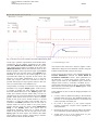
Each part of the tool is further divided into several sections
represented in Figures 3 and 4, which show the two main
screens of the interactive tool.
3.1 Model identification screen
The Model Identification screen is shown in Figure 3. This
screen is focused on determining the K, T, and L parameters
of a first order with a dead time model (FOPDT). The process
transfer function to be identified can be modified depending
on the option selected from the Settings menu. Several
examples of transfer function are given, and its parameters
can be modified interactively by dragging sliders or setting
specific values using text-edits fields. However a free transfer
function can be selected (Interactive TF option in the
Settings menu) where the process poles and zeros can be
inserted, removed or changed from the Process Transfer
Function graphic. All these elements are available in the lefthand area of the screen. In the right-hand of the screen, there
are different graphical elements.
IFAC Conference on Advances in PID Control
PID'12
Brescia (Italy), March 28-30, 2012
WeB2.6
Process step response
Model step response
Fig. 3. Interactive tool user interface for model identification phase
On the top a symbolic representation of the model shows
continuously all the changes performed on the model
parameters (Model transfer function). With this purpose
some sliders and text-edits are available in the same area
(Model parameters). Below these elements, there are two
different graphics which represent the input signal (Input)
and the process step response of the system (Output) to be
identified in red colour. In the second graph it is also
represented the model step response in blue colour. The
objective of the model identification is to try that the
model step response (blue line) coincides as much as
possible with the process step response (red line). The user
can try to fit the model in two different ways.
One possibility to modify in an interactive way the model
parameters is by using the Output graphic. In this sense, it
is possible to modify the static model gain using the
horizontal dashed blue line in the Output graphic. The
model time constant and the model delay can also be
changed using the vertical blue dashed lines in the Output
graphic. These options allow the user to find an adequate
model for the given process transfer function. A second
alternative is using the sliders and text-edits that are
available in the Model parameters area. In both cases an
optimal model can also be fitted to the given process
transfer function using the option called Optimization
fitting in the Setting menu. This option uses an
optimization algorithm, which tries to obtain the best
model for the given data. On the top right corner of the
Input graphic the mean square error between the model
output and the process output is shown being a reference
measurement to obtain the desired model.
3.2 Control design screen
The second screen of the tool is shown in Figure 4 and is
dedicated to design the event-based PI controller using the
FOPDT model obtained in the previous stage.
In the left part of the screen it is now included besides the
Process Parameters elements the Event Based PI
Controllers Parameters section. These parameters are
the following:  = speed of the process response,  =
upper (lower) limit of the deadband region where the
integral action of the Cfb controller is enabled, KpTi =
proportional (integral) action of the Cfb controller. Below
these elements we include again the Output graphic of the
Model identification screen.
Some guidelines on how to tune the design parameters can
be outlined:
 yll and yul must be defined according to the maximum
tolerable steady-state error. The deadband should wrap
the noise in a real implementation to avoid trains of
events, especially from the P part.
 If yll and yul are equal to ysp, the system response
oscillates around the set-point value regardless the
other parameters.
 Increasing the values of P and I reduces the number
of events and the speed and damping of the response.
 A high value of P or I can cancel the P or I part,
respectively, as events are not triggered.
IFAC Conference on Advances in PID Control
PID'12
Brescia (Italy), March 28-30, 2012
WeB2.6
Fig. 4. Interactive tool user interface for event based PI controller design phase
Åström, K. J. (2007) Event based control. In A. Astolfi
 The cancellation of the P part because of a high value
and L. Marconi, editors, Analysis and Design of
of P introduces oscillations in the loop.
Nonlinear Control Systems. Springer Verlag.
 A good compromise between the number of events and
Åström, K. J. and B. Wittenmark (1997). Computer
the control performance is obtained with P and I
controlled systems: Theory and design. Third Edition.
ranging from 2% to 10% of ysp.
Prentice Hall. New Jersey.
Feency, L. M. and M. Nilsson (2001). Investigating the
Figure 4 shows an example of the method applied to a
energy comsumption of a wireless network interface
second order process P(s) = 2.5/((1+ s) (1+ 0.5s)) with a
in an ad hoc networking environment. Proceedings of
unit load disturbance step at t = 3.8. The PI parameters
IEEE Infocom, 1548-1557.
Kp = 0.95 and Ti = 0.87 have been determined by applying
Heemels, W.P.M.H., Sandee, J., and van den Bosch, P.
the well-known SIMC tuning rules (Skogestad, 2003)
(2008). Analysis of event-driven controllers for linear
systems. Intern. J. of Control, 81(4), 571–590.
5. CONCLUSIONS
Miskowicz, M. (2006). Send-on-delta concept: An eventbased data reporting strategy. Sensors 6(1), 29-63.
A new interactive tool for analysis and design of a new
Piguet,
Y. (2004). SysQuake 3 User Manual. Calerga
2DOF event based PI controller has been described. The
S‘arl,
Lausanne (Switzerland).
purpose is to enhance the knowledge of these kind of
Sánchez,
J.,
A. Visioli and S. Dormido (2011). A twosystems by exploiting the advantages of immediately
degree-of-freedom
PI controller based on events.
seeing the effects of changes that can never be shown in
Journal of Process Control, 21, 639-651.
static pictures. The module has been implemented in
Skogestad, S. (2003). Simple analytic rules for model
Sysquake, a Matlab-like language with fast execution and
reduction and PID controller tuning. Journal of
excellent facilities for interactive graphics.
Process Control, 13 (4), 291–309.
Visioli, A. (2004). A new design for a PID plus
ACKNOWLEDGMENT
feedforward controller. Journal of Process Control, 14
(4), 455–461.
This work was supported by the Spanish CICYT funds
Visioli, A. (2006). Practical PID Control. Springer,
under Grant DPI2007-61068
London, UK.
Wittenmark, B., H. Häglund, and M. Johansson (1998)
REFERENCES
Dynamic pictures and interactive learning, IEEE
Årzén, K. J. (1999). A Simple event-based PID controller.
Contr. Syst. Mag., 18 (3), 26–32.
Proceedings of 14th IFAC World Congress. vol. 18.
Beijing, China. 423-428.