Download fulltext - DiVA Portal

Robust control solutions for stabilizing
flow from the reservoir: S-Riser
experiments
Mahnaz Esmaeilpour
Abardeh
Chemical Engineering
Submission date: June 2013
Supervisor:
Sigurd Skogestad, IKP
Co-supervisor:
Ole Jørgen Nydal, EPT
Esmaeil Jahanshahi, IKP
Norwegian University of Science and Technology
Department of Chemical Engineering
Robustcontrolsolutionsforstabilizing
flowfromthereservoir:S‐Riser
experimentsandsimulations
MahnazEsmaeilpourAbardeh
June26,2013
Preface
ThisthesisiswrittenasthefinalpartofmyMasterdegreeinChemicalEngineering
attheNorwegianUniversityofScienceandTechnology(NTNU),classof2013.
I would like to express my greatest gratitude to my highly knowledgeable
supervisor, professor Sigurd Skogestad, for all his helps, his good guidance and
encouragements. I am also grateful to my co‐supervisors, professor Ole Jorgen Nydal
and PhD student Esmaeil Jahanshahi, who helped and supported me throughout my
thesis. It has been a great opportunity and honor for me to be part of your team in
generatingnewideasandIamconfidentwhatIhavelearnedthroughthisthesiswillbe
surelyusedinpracticeinmyprofessionalcareer.
DeclarationofCompliance
I, Mahnaz Esmaeilpour Abardeh, hereby declare that this is an independent work
according to the exam regulations of the Norwegian University of Science and
Technology(NTNU).
Dateandsignature:
i
Abstract
One of the best suggested solutions for prevention of severe‐slugging flow
conditionsatoffshoreoilfieldsistheactivecontroloftheproductionchokevalve.This
thesis is a study of robust control solutions for stabilizing multiphase flow inside the
risersystems;throughS‐riserexperimentsandOLGAsimulations.“Nonlinearity”asthe
importantcharacteristicofsluggingsystemposessomechallengesforcontrol.Focusof
thisthesisisononlinetuningrulesthattakeintoaccountnonlinearityoftheslugging
system.Themainobjectivehasbeentoincreasethestabilityofrisersystemsathigher
levelsofvalveopeningswithmoreproductionrates.
Similarresearchhasbeendonepreviously,butisrepeatedinthisthesisusingnew
systematic tuning methods. Three different tuning methods have been applied in this
thesis. One is Shams’s set‐point overshoot method developed by Shamsozzhoha
(ShamsuzzohaandSkogestad2010).TheotherisIMC‐(InternalModelControl)based
tuningmethodwithrespecttotheidentifiedmodelofthesystemfromclosed‐loopstep
test.ThelasttuningmethodissimplePItuningruleswithgainschedulingforthewhole
operating range of the system considering the nonlinearity of the static gain. The two
latter methods have been developed very recently by Jahanshahi and Skogestad
(JahanshahiandSkogestad2013).
Twoseriesofexperimentshavebeencarriedoutusingamedium‐scaletwo‐phase
flow S‐riser loop. A single loop control scheme with riser‐base pressure as the
measurementwasused.Therobustnessofdifferenttuningmethodswascomparedby
slowlydecreasingtheset‐pointoftheclosed‐loopsystem,whichwastheinletpressure,
until instability was reached. The choke valve opening was increasing gradually by
decreasing the set‐point. A control with a robust tuning method can maintain system
stability in a large range of conditions. The choke valve was then replaced with a
quicker valve after the first set of experiments. The same experiments were repeated
andtheeffectofcontrolvalvedynamicswasinvestigatedthereafter.
The experiments were simulated in OLGA and the same control tests were
performed.TheOLGAcasewasconstructedbasedonthefirstseriesoftestswithvalve
1andthedesignedcontrollerswithdifferenttuningstrategieswereapplied.Resultsof
theexperimentsverifiedthoseofthesimulations.
The tuning method with the highest robustness was thus the one which could
stabilizethesystematthelargestchokevalveopening(thelowestinletpressure).The
besttuningmethod,withrespecttorobustnessisthesimplePItuningruleswithgain
scheduling for the whole operating range of the system. With this method, it was
possibletostabilizetheexperimentalrisersystemuptoachokevalveopeningof37%
from an open‐loop stability of 16 %. It was also able to stabilize the simulated riser
systemuntilachokevalveopeningof75%fromanopen‐loopstabilityof26%.
Top side measurements were in general difficult to use in anti‐slug control.
Measurement of the topside density using a conductance probe installation was not
successful.Therefore,nocascadeanti‐slugcontrolschemescouldbetested.
ii
iii
Contents
Preface.....................................................................................................................................................i Abstract.................................................................................................................................................ii 1 Introduction................................................................................................................................1 1.1 2 3 Scopeofthethesis...........................................................................................................................2 Background.................................................................................................................................3 2.1 Multiphasetransport.....................................................................................................................3 2.2 Slugflow..............................................................................................................................................5 2.3 Riserscontainingmultiphaseflow...........................................................................................6 2.4 Riserslugging....................................................................................................................................7 2.5 Anti‐slugoperations.....................................................................................................................11 2.5.1 Choking.....................................................................................................................................11 2.5.2 Gaslift........................................................................................................................................11 2.5.3 Slugcatchers...........................................................................................................................12 2.5.4 Activecontrol.........................................................................................................................12 2.6 Modelingofrisersystems..........................................................................................................13 2.7 Bifurcationdiagrams....................................................................................................................13 2.8 PIDandPIcontrollers..................................................................................................................14 2.9 TuningofPIDandPIcontrollers.............................................................................................15 2.9.1 Method1:Shams’sset‐pointovershootmethodforclosed‐loopsystems..15 2.9.2 Method2:TuningbasedonIMCdesign......................................................................18 2.9.3 Method3:SimpleonlinePItuningmethodwithgainscheduling...................22 Experimentalwork................................................................................................................26 3.1 SetupDescription..........................................................................................................................27 3.2 Equipment........................................................................................................................................30 3.2.1 Mainwaterstoragetank....................................................................................................30 3.2.2 Airreservoirtank.................................................................................................................31 iv
4 3.2.3 Airbuffertank........................................................................................................................32 3.2.4 Overflowtank.........................................................................................................................33 3.2.5 Pressuretransmitters.........................................................................................................33 3.2.6 Smallseparator......................................................................................................................34 3.2.7 Centrifugalwaterpump.....................................................................................................34 3.2.8 Airflowmeter........................................................................................................................35 3.2.9 Waterflowmeter..................................................................................................................35 3.2.10 Chokevalves.......................................................................................................................37 3.2.11 Conductanceprobe(C)..................................................................................................38 3.2.12 LabVIEW..............................................................................................................................39 Simulationofexperimentalcases....................................................................................41 4.1 OLGA®,multiphasesimulationtool.......................................................................................41 4.2 Constructionofthecase.............................................................................................................41 4.2.1 Flowpathgeometry.............................................................................................................42 4.2.2 Fluidproperties.....................................................................................................................43 4.2.3 Boundaryandinitialconditions.....................................................................................43 4.2.4 Numericalsetting.................................................................................................................44 4.3 5 Resultsanddiscussion.........................................................................................................46 5.1 Experimentalresults....................................................................................................................46 5.1.1 Seriesofexperimentswithvalve1(slowchokevalve)........................................47 5.1.2 Seriesofexperimentswithvalve2(fastchokevalve).........................................57 5.1.3 CascadeControlusingtoppressurecombinedwithdensity............................68 5.2 ComparisonofSlowvalveandFastvalve...........................................................................70 5.3 SimulatedresultsfromOLGAmodel.....................................................................................74 5.3.1 Open‐loopsimulations.......................................................................................................74 5.3.2 Controlbytrialanderror..................................................................................................75 5.3.3 Tuningthecontroller..........................................................................................................79 5.4 ImplementingPIDcontrollerinOLGA.................................................................................44 Comparisonofexperimentalandsimulatedresults......................................................95 5.4.1 Open‐loopbifurcationdiagrams....................................................................................95 5.4.2 ComparisonofcontrolresultsfromIMC‐basedtuningmethod......................96 5.4.3 ComparisonofcontrolresultsfromSimpleonlinetuningmethod................96 5.4.4 Comparisonoftuningmethods......................................................................................97 v
6 7 8 Discussionandfurtherworks........................................................................................100 6.1 Tuningmethods..........................................................................................................................100 6.2 Controlstructures......................................................................................................................101 6.3 Discussableissuesrelatedtoexperimentalactivities................................................102 6.3.1 Oscillationsinflowrates................................................................................................102 6.3.2 Waterflowbackintothebuffertank........................................................................102 6.3.3 Leakageinsteelconnection..........................................................................................102 Conclusion..............................................................................................................................104 7.1 Stabilizingcontrolexperimentsusingbottompressure...........................................104 7.2 TestingonlinetuningrulesonS‐riserexperiments....................................................104 7.3 Controlusingtoppressurecombinedwithdensity....................................................105 7.4 Investigatingeffectofcontrolvalvedynamics..............................................................105 7.5 ControlsimulationsusingOLGA..........................................................................................106 References..............................................................................................................................107 A.LowpassfilterinLabVIEW..............................................................................................109 B. SimulatedresultstogetthebeststeptestsforShams’smethod.....................110 C. SomeexamplesofMATLABscripts..............................................................................111 vi
vii
1 Introduction
MultiphasepipelinesareacommonfeatureofoffshoreproductionintheNorthSea.
Theyconnectsubseawellstothetopsideprocessingfacilitiesortheplatforms.Inmany
points of transportation, these pipelines get the shape of L‐shaped or S‐shaped risers.
The stability of multiphase flow inside these pipeline‐riser systems is of great
importance and many efforts have been spent on this issue so far. In low reservoir
pressuresorlowflowrateconditionstheliquidphasestendtoaccumulateinlowpoints
and form liquid slugs. This leads to the pipeline or riser blockage and can be more
dangerous when the length of slugs is comparable to the length of the riser. This
phenomenon is called Severe slugging (also Terrain slugging or Riser slugging) and is
characterizedbylargeoscillatoryvariationsinpressureandflowrates(Storkaas2005).
These large variations lead to a poor separation, unwanted flaring and even a plant
shutdownintheworstcase.
Reducingopeningofthetopsidechokevalvehasbeenatraditionalwaytosuppress
severe slugging. However, this increases the valve back pressure and therefore
decreasestheproductionratefromthewell.
Activefeedbackcontrolofthetopsidechokevalvecanmakeitpossibletostabilize
theflowattheconditionswherenormallyseveresluggingispredicted.Thisreducesthe
need for additional topside equipment and allows a higher rate of oil recovery. The
control system is called anti‐slug control and its main objective is to keep the
multiphaseflowasstableaspossiblebymanipulatingthetopsidechokevalveusingthe
parameterssuchaspressureordensityasthecontrolvariables.
In the way of developing new technologies for stabilizing control of severe
slugginginrisersystemsmanyresearcheshavebeendoneattheNorwegianUniversity
ofScience andTechnology.Thework hasbeenguided bySkogestad(Skogestad2003;
Storkaas 2005; Shamsuzzoha and Skogestad 2010; Jahanshahi and Skogestad 2011;
Skogestad and Grimholt 2011; Jahanshahi and Skogestad 2013) and performed at the
department of Chemical Engineering. Storkaas (Storkaas 2005), Sivertsen (Sivertsen
2008), Jahanshahi (Jahanshahi and Skogestad 2011) and numerous master students
haveworkedonmodelingandcontrollingofrisersystems.
1
Companies like ABB (Havre, Stornes et al. 2000), Statoil and Total have all
researched prevention of slugging and built installations at offshore locations. Statoil
completed in 2001 their first slug control installation at the Heidrun oil platform.
Siemens is also involved in slugging research and funds a PhD program, which this
thesisisconnectto.
Intheanti‐slugcontrolsystem,itisveryimportantthatthecontrollersarefine
tuned. Otherwise, the control system is not robust in practice and the closed‐loop
systembecomesunstableafteraplantchange.Thesluggingsystemishighlynonlinear
sincethegainchangesat differentoperatingpoints.Forsuchasystemthecontrollers
needtoberetunedateachoperatingpoint.
1.1
Scopeofthethesis
Inthisthesisthreedifferenttuningmethodswillbetestedwithexperimentsand
simulations to find the most robust solution for anti‐slug control system. High
robustnesswillbeobtainedifthesystemcanmaintainstabilityatlargedeviationsfrom
openloopconditions.Thismeanslargechokevalveopenings.Thetuningmethodsare
systematicandhavebeendevelopedveryrecently(ShamsuzzohaandSkogestad2010;
JahanshahiandSkogestad2013).
TheexperimentsofthisthesiswillbecarriedoutatthedepartmentofEnergyand
ProcessEngineering.Twoseriesofexperimentswillberunusingamedium‐scaletwo‐
phase flow S‐riser loop. The difference between the two series is the type of choke
valve.Theaimistoinvestigatetheeffectofcontrolvalvedynamicsonperformanceof
the control system in addition to robustness of the tuning methods. Possibility of
differentcontrolstructureswillbealsoinvestigated.
The experiments will be simulated in multiphase flow simulator, OLGA, and the
same control tests will be performed. Finally the simulated and experimental results
willbecompared.
2
2 Background
2.1
Multiphasetransport
Whenitcomestooffshoreproductionofoilandgas,longtransportofmultiphase
flowhasrecentlybecomeofgreatattention.Manypipelinesandrisersarecarryingthe
combination of natural gas, condensate, oil and water from the North Sea to shore.
Previously, large production platforms equipped with process facilities were built on
the sea floor with the aim of separating gas, oil and water. Today this can be too
expensive and multiphase transportation can save billions of dollars for the oil
companiesinstead.
Design and operation of multiphase transportation systems raise many new
challenges. These challenges could be either related to the flow, fluid or the pipe
integrity. Pressure drop/ boosting, Slugging, liquid emulsion, temperature change,
scaling, hydrate and wax formation can be examples of them. Overcoming these
challengesandhavingasafeanduninterruptedmultiphaseflowreferstotheterm“flow
assurance”. This term was first used by Petrobras in the early 1990s and it originally
referred to only thermal hydraulics and production chemistry issues encountered
duringoilandgasproduction(Fabre,Peressonetal.1990).
One important issue in flow assurance is stabilizing the multiphase flow inside
the pipeline‐riser systems. From a control engineering point of view, this can be
referred as control of the disturbances in the multiphase flow as the feed to the
separationprocess.Avoidingvariationsintheflowenteringtheprocessingunit,atthe
outlet of the multiphase pipelines is the issue of interest for control (Bratland 2010).
The ability of predicting the flow patterns and reserving a stable flow is of great
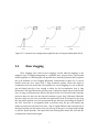
importance, which is the objective of the thesis. Figures 2.1 and 2.2, adapted from
Bratland (Bratland 2010), describe possible flow patterns inside the horizontal and
verticalpipelines.
3
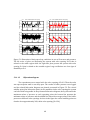
Figure2.1:Gas‐liquidflowregimesinhorizontalpipes.
Figure2.2:Gas‐liquidflowregimesinverticalpipes.Slugflowisthepointofinterestin
thethesis.
Changingmultiphaseflowbetweendifferentflowregimescanbedescribedbya
typical flow regime map shown in figure 2.3, adapted from Taitel (Taitel 1986). The
boundariesbetween stableand unstableregionsare clearlyshownin theflowregime
map. With applying feedback control these boundaries can be moved and thereby the
stableregioncanbeincreased.
4
or multiph
hase flow (Taitel
(
198
86). Stabilitty boundarries are
Figure 2.3: Stabillity map fo
clearlyshownintthemap.
2.2
Slu
ugflow
w
A
Among th
he flow asssurance concerns,
c
managemeent of slu
ugging in system
Fard et al.. 2005).
deliverrability hass received m
much interrest in receent years (Godhavn,
(
Slugflo
owisoneo
oftheflowp
patternsch
haracterizeedbyaltern
natingslugsofgasandliquid
flowingginthepip
pes.Inthis typeofflo
owregime, elongated bubblesoffgasseparratedby
“slugs” ofliquid,ttravelfrom
moneendo
ofthepipettotheotheerend.Itcaanbeeitherrdueto
differen
ntvelocitieesofgasan
ndliquidphasewhich
hisreferreedashydro
odynamicsslugging
or pipeeline geom
metry which
h is referreed as terraain induced
d slugging. The latterr one is
commo
on in riserss and its main
m
reason
n is the gravity. A schematic map
m of slug flow is
shown infigure2
2.4,adapted
dfrom(Yan
nandChe2
2011).The masterunfavorableeeffectof
slug flo
ow is its instability
i
that has a
a negative impact on
n the operration of offshore
o
producction facilitties. The periodic
p
oscillations o
of liquid and
a
gas ph
hases due to
t their
inhomo
ogeneous distribution
d
n cause oscillatory pressures
p
and decreeases the level
l
of
producction as laarge as 50
0%. The average of these osccillations iss lower th
han the
equilibrium prod
duction an
nd this giives the production
p
n losses. More
M
overr these
oscillattions can damage th
he pipe an
nd the separation process.
p
Fo
or these reasons,
r
5
suppressingtheslugflowisofdominantimportance.Ahomogeneoussteadyflowwith
very small bubbles of gas well distributed in the continuous liquid phase is most
desired.Insuchdesiredsituation,thepressureremainsconstantovertime.
Figure 2.4: Schematic map of slug flow in a vertical pipe in a slug unit (Yan and Che
2011)
2.3
Riserscontainingmultiphaseflow
Risers are a special type of pipeline developed for vertical transportation of
materialsfromseafloortoproductionanddrillingfacilitiesonthewater'ssurface.They
canbeintypesofrigidrisers,flexiblerisersandhybridrisersthatisacombinationof
the rigid and flexible. Risers can have many different configurations. However in this
thesisalltheS‐shapedtypesarethepointofinterestregardlessoftheirdifferences.The
functionalsuitabilityandlongtermintegrityoftherisersystemaffectstheselectionof
riserconfiguration(Bai2001).Figure2.5showsprevalentriserconfigurations.
6
Figure2.5:Commonriserconfigurationsappliedintheoilandgasindustry(Bai2001)
2.4
Riserslugging
Riser slugging (also called severe slugging/ terrain induced slugging) is the
toughest type of slugging happening in a pipeline‐riser system where a downward
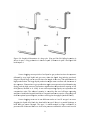
inclinedpipelineisconnectingintoanupwardriser.Storkaas(Storkaas2005)explains
the cyclic behavior of riser slugging illustrated schematically in figure 2.6. It can be
broken down into four steps. Step 1: Slug formation: gravity causes the liquid to
accumulateinthelowpointandaprerequisiteforseveresluggingtooccuristhatthe
gas and liquid velocity is low enough to allow for this accumulation. Step 2: Slug
production:Theliquidblocksthegasflow,andacontinuousliquidslugisformedinthe
riser.Aslongasthehydrostaticheadoftheliquidintheriserincreasesfasterthanthe
pressuredropovertheriser,theslugwillcontinuetogrow.Step3:Blowout:Whenthe
pressure drop over the riser overcomes the hydrostatic head of the liquid in the slug,
theslugwillbepushedoutofthesystemandthegaswillstartpenetratingtheliquidin
the riser. Since this is accompanied with a pressure drop, the gas will expand and
furtherincreasethevelocitiesintheriser.Step4:Liquidfallback:Afterthemajorityof
theliquidandthegashaslefttheriser,thevelocityofthegasisnolongerhighenough
to pull the liquid upwards. The liquid will start flowing back down the riser and the
accumulationofliquidstartsagain.
7
Figure 2.6:Graph
hicalillustrrationofa slugcycle (Yanand Che2011)).Slugform
mationis
shown in part 1. Slug produ
uction is sh
hown in paart 2, Blow
wout in parrt 3 and liq
quid fall
backin
npart4.
Severeslugggingcausesperiods ofnoliquiidorgasproduction intotheseeparator
followeed by very
y high liquiid and gass rates, wh
hen the liq
quid slug iss being produced.
Lengthofliquidsslugscanb
beseveralttimestheleengthofth
heriser.Th
hisphenom
menonis
highlyu
undesirablle.Thelarggeliquidprroductionm
mightcauseeoverflow andshutd
downof
thesep
parator.Flu
uctuations ingasprod
ductionmigghtcauseo
operationalproblemssduring
flaring,,andthehighpressurefluctuattionsmighttreduceth
heproductioncapacity
yofthe
field(Jaansen,Sho
ohametal. 1996).Itccanreduceeoperatinggcapacityfforseparattionand
compreession unitts. The red
duced capaacity is cau
used by th
he need off larger op
perating
margin
nstohandleethelargerrdisturban
nces.Largerrdisturban
ncesrequirrealargerb
back‐off
fromth
heoptimaloperationp
point,andtthusreducingthethroughput(SStorkaas20
005).
occurintw
wodifferen
ntmodesoffIandII.IIntypeIoffsevere
Severeslugggingcano
sluggin
ng the liquiid fully blo
ock the ben
nd while in
n type II th
here is a partial
p
blocckage at
bend and
a
gas paasses throu
ugh. The type
t
I is characteriz
c
zed by larrge oscillattions in
pressurreandacceeleratedblo
owout.Infactthepreessureosciillationsreflectstaticheadof
8
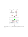
theriser.TherearesmallpressureoscillationsintheseveresluggingoftypeIIandthe
sluglengthisshorterthantheheightoftheriser.Butflowoscillationscanbelarge.Type
IIsluggingisnotusuallycriticalforastableoperation.Figures2.7and2.8,adaptedfrom
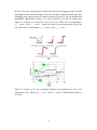
Malekzadeh (Malekzadeh, Henkes et al. 2012), illustrate SS1 and SS2 respectively.
Figure 2.7 is based on a measured cycle of the riser P for SS1 corresponding to
U SL  0.20 ms 1 and U SGO  1.00 ms 1 .Figure2.8isbasedontheexperimentalcycleforthe
riser P ofSS2correspondingto U SL  0.10 ms 1 and U SGO  2.00 ms 1 .
Figure 2.7: Stages for SS1 (a) a graphical illustartion (b) marked on a cycle of an
experimental riser P trace ( U SL  0.20 m s  1 and U SGO  1.00ms 1 ) (Malekzadeh, Henkes et
al.2012)
9
Figure 2.8: Stages for SS2 (a) a graphical illustartion (b) marked on a cycle of an
experimentalriser P trace( U SL  0.10 ms 1 and U SGO  2.00 ms 1 )(Malekzadeh,Henkesetal.
2012)
10
2.5
Anti‐slugoperations
Asthefieldsbecomemorematurethemoreadvancedtechnologyisdemanded.
Thereasonisthattheenergyofreservoirdecreasesduetoitsaging.Thisleadstolower
pressureandtemperaturesinreservoir.Thelowerpressureofreservoircauseslimited
drivingforcetotheflowandtherebylowerphasevelocitiesinresultandfinallymore
probable riser slugging formation. Low temperatures also increase the probability of
solidformation.Changingthedesignofpipe‐risersystemtoavoidsluggingcannotbe
economicallyfeasible.Themostcommonmethodsforavoidingsluggingarepresented
below.
2.5.1
Choking
Schmidt et al. (1979) first suggested choking (decreasing the opening Z) of the
valveattherisertopasaneliminationwayofsevereslugging.Thetheorybehindthis
suggestionisthatthesteadyflowisgainediftheaccelerationofthegasabovetheriser
is stabilized before reaching the choke valve (Jansen, Shoham et al. 1996). This
increasesthebackpressureandthevelocityatthechokethereupon.Themechanismis
explainedasapositiveperturbationintheliquidholdupinapipeline‐risersystemwith
astableflowwillincreaseweightandwillcausetheliquidto“falldown”.Theresultof
this is an increased pressure drop over the riser. The increased pressure drop will
increasethegasflowandpushtheliquidbackuptheriser,resultinginmoreliquidat
thetop of the riser than prior totheperturbation. With a valve opening larger than a
certaincriticalvalue(Zcrit)toomuchliquidwillleavethesystem,resultinginanegative
deviation in the liquid holdup that is larger than the original positive perturbation.
Thus,wehaveanunstablesituationwheretheoscillationsgrow,resultinginslugflow.
ForavalveopeninglessthanthecriticalvalueZcrit,theresultingdecreaseintheliquid
holdupissmallerthantheoriginalperturbation,andwehaveastablesystemthatwill
returntoitsoriginal,non‐sluggingstate(Storkaas2005).
2.5.2
Gaslift
Gaslifthasbeensuggestedasanothermethodofeliminatingsevereslugging.In
thismethodthehydrostaticheadoftheriserisreducedwithgasinjectionandthusthe
pipelinepressurewillbereduced.Theinjectedgasliftstheliquidtowardsuptheriser.
If sufficient gas is injected the liquid will be continuously liftedand a steady flow will
occur.Thedrawbackofgasliftisthelargegasvolumesneededtoobtainasatisfactory
stabilityoftheflowintheriserandthisistooexpensive(Storkaas2005).
11
2.5.3
Slugcatchers
Oneotherwaytoaccommodatesluggingiscommontoinstallalargeseparator
asaslugcatcherattheexitofthepipeline.Theslugcatcheristhefirstelementinthe
processing facility and determining its proper size is vital to the optimal operation of
theentirefacility.Thefundamentalpurposeofslugcatcheristoremovefreegasfrom
the liquid phase and to deliver a relatively even supply of liquid to the rest of the
production facility. An advantage of this set‐up is that inspection and maintenance on
the slug catcher can be done without interrupting the normal operation. There are
mainlytwotypesofslugcatchers,thevesselandthemultiple‐pipetypesandtheuseof
each type depends on the type of flow stream. Multiple‐pipe separators have been
widelyappliedingas‐condensateprocessingfacilities(Miyoshi,Dotyetal.1988).
Installingslugcatchershasseveraldrawbacks;itputsalowerboundontheoperating
pressureofthepipe,whichagainlimitstheflowfromthereservoir.Italsoincreasesthe
mechanical wear of the pipeline due to large oscillations in pressure. The capital and
maintenancecostsofaslugcatcherarerelativelylarge(Olsen2006).
2.5.4
Activecontrol
Risersluggingcanbepreventedusingstabilizingfeedbackcontrol.Anapproach
basedonfeedbackcontrolwasfirstproposedbyShmidt(Shmidtet.al.1978).Theidea
ofpaperwastosuppressterrainsluggingbyusingthetop‐sidechokevalveandasimple
feedback loop, measuring pressure at the inlet and upstream the riser or the top
pressure before the choke valve as inputs. With feedback control, the stability of the
flowregimescanbechangedtoenhanceoperation.Infacttheboundariescanbemoved
via feedback control, thereby stabilizing a desirable flow regime where riser slugging
“naturally”occurs(Storkaas2005).Anti‐slugcontrolcanmove theboundariesinflow
regime map resulting in increased stable region. It sounds to be one of the best
solutions for prevention of severe‐slugging. Several models have been suggested by
researchers to describe the system dynamics and several controllers have been
designed.Themodelsaremeanttoaidtuningofcontrollerswhichusetheproduction
chokevalveastheactuatorandtrytostabilizethesystemwithamoreproductionrate
in a higher valve opening. The objective could be defined as obtaining the most
robustness for the system against large inflow disturbances. “Nonlinearity” as the
important characteristic of slugging system provides some challenges for control.
However, a good control system using a model that is most consistent with the plant
couldhavegoodresultsinachievingdesiredstableflowregimes.
12
2.6
Modelingofrisersystems
Themainobjectivesofmodelingofproductionflowinpipelinesandrisersareto
predict the pressure drop, the phase distributions, the potential for unsteady phase
delivery(slugging) and the thermal characteristics of the system (Pickering,Hewitt et
al. 2001). The reliability of these simplified models is however questionable. The
analysisandmodelingofmultiphaseflowsreliesheavilyonempiricalcorrelationsand
thepredictionsforthemodelsareonlyasreliableastheempiricaldataonwhichthey
arebased.Thereforeitcanbequestionedwhetherthemodelswouldbevalidifapplied
torealsystems.Theyaretestedbytheuseofsmalldiametersexperimentalrisersand
maybemorethangoodenoughforsuchsystems,buttheystillmaybeinvalidforusein
largersystems(Pickering,Hewittetal.2001).
The tuning methods used in this work are provided via linear and nonlinear
multiphase flow models based on the mass balances over the different sections of the
pipeline‐risersystem.Thesimplifiedfour‐statemechanisticmodelmadebyJahanshahi
andskogestad(JahanshahiandSkogestad2011)usessimplerelationshipstocalculate
thephasedistributionsoverthedifferentsectionsofsystem.Themodelhasbeenthen
linearizedaroundanunstableoperatingpointandafourth‐orderlinearmodelwithtwo
unstable poles, two stable poles and two zeros is produced. Since a model with two
unstable poles is enough for control design, the model order is reduced by using
balancedmodeltruncationviasquarerootmethod.Thisidentifiedmodelofthesystem
is then used for an IMC (Internal Model Control) design and finding new IMC‐based
tuningrules.(JahanshahiandSkogestad2013).Moreover,asimplemodelforthestatic
nonlinearity of the system is proposed by Jahanshahi and based on this static model,
simplePItuningrulesconsideringnonlinearityofthesystemaregiven(Jahanshahiand
Skogestad2013).Thesetuningruleshavebeenusedinthesimulationsandexperiments
ofthisthesisandaclearcomparisonoftheresultshavebeenpresented.
2.7
Bifurcationdiagrams
Bifurcation diagrams have been used in this thesis in order to plot the values of
pressureversusthevaluesofvalveopeningforthesluggingsystemeitherinopen‐loop
positionorinclosed‐looppositionwithdifferentcontrollers.Bifurcationdiagramsare
thesimplestwaytoillustratethestabilityofthesystem.Inthestableregionstheplot
consistsofaunitcurveshowingtheexactvalueofthepressure(insimulations)orthe
average of very small pressure oscillations (in experiments) while in the unstable
regions the plot consists of three curves, one for steady state conditions and the two
others showing the maximum and minimum of oscillations at each value of valve
openingovertheworkrangeofchokevalve.
13
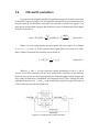
2.8
PIDandPIcontrollers
PI(proportional‐integral)andPID(Proportional‐integral‐derivative)controlare
oftheearliercontrolstrategies.ThePIDcontrollerincludestheproportionalaction(P),
integralaction(I),andderivativeaction(D).Thecontrollerusestheerrorsignal e ( t ) to
generatetheproportional,integral,andderivativeactions.Amathematicaldescription
ofthePIDcontrolleris:
1
u (t )  K p [ e ( t ) 
Ti
de(t )



e
(
)
d
(
)
T
]
d
0
dt t
Equation2.1
Where u ( t ) istheinputsignaltotheplantmodel.Theerrorsignal e ( t ) isdefined
as e (t )  r (t )  y (t ) and r ( t ) isthereferenceinputsignal(Fabre,Peressonetal.1990).
AfteraLaplaceTransformthecontrollercanbeshownas:
c  K c (1 
1
  s)
Is d Equation2.2
Where Kc ,  I and  d are the respective tuning parameters for the P, I and D
actions. PI and PID controllers are the most widely used controllers in the industry.
However,theyneedtobetunedappropriatelyforrobustnessagainstplantchangesand
large inflow disturbances. (Jahanshahi and Skogestad 2013) Thus finding the most
appropriateamountsof Kc ,  I and  d couldbeextremelyrequired.Atypicalstructureof
aPIDcontrolsystemisshowninFigure2.9.
Figure2.9:AtypicalPIDcontrolstructure
14
2.9
TuningofPIDandPIcontrollers
Many tuning methods for different systems have been introduced so far by
researchers andengineers.Dependingon thecharacteristics ofthe system(plant), for
instancenonlinearityandstability,differentlevelsofrobustnessisachievedbydifferent
tuningmethods.Threedifferenttuningmethodshavebeenappliedinthisthesis.Twoof
them are quite new and have been recently developed (Jahanshahi and Skogestad
2013).Theyarespecifiedforthesluggingsystem.Infact,thisthesisisaverificationof
thesenewmethods.
2.9.1
Method1:Shams’sset‐pointovershootmethodfor
closed‐loopsystems
Some systems like slugging system are originally unstable in open‐loop. For
these systems model from closed‐loop response with P‐controller can be used to find
the appropriate tuning parameters. A method called “Shams’s set‐point overshoot
method” was first constructed by Shamsuzzoha et al. (Shamsuzzoha and Skogestad
2010).Skogestadetal.(Skogestadand Grimholt 2011)developedthismethodfurther
intoatwo‐stepclosed‐loopprocedure.Astepbystepdescriptionofthetwostepclosed‐
loopShams’smethodispresentedbelow.
Theclosed‐loopsystemwithP‐controllershouldbeatsteady‐stateinitially,that
is,beforetheset‐pointchangeisapplied.Then,aset‐pointchange,  y s ,isapplied.The
step change and the P controller gain ( Kc0 ) should be adjusted in a way that the
overshoot (D) is approximately 30 %. Figure 2.10 shows a graphical illustration and
equation2.4findstheovershoot.
15
w
P‐only
y controller (Skogesttad and
Figure 2.10: clossed‐loop seet‐point reesponse with
olt2011)
Grimho
onfromtheegraphicallsteprespo
onse:
Extracttinformatio

Timetofirrstpeak: t p 
Maximumoutputchaange:  y p 
Relativestteadystateoutputchaange:

Alternativeely,  y  caanbeestim
matedfromequation2
2.6,usingth
heoutputch
hange
 y  atfirstund
dershoot( yu ):
y  0.45( y p   yu ) 
Overshoott:
D

y p  y
y
Equattion2.4
Steadystatteoffset:
B
Equatiion2.3
 y s   y
 y
16
Equattion2.5

Theparameter(A):
A  1.152 D 2  1.607 D  1 Equation2.6
 Theparameter(r):
r
2A
B
Equation2.7
Thefirstorderplusdelaymodelparameters:

Steadystategain:

k
1
Kc0 B
Equation2.8
Delay:

  t p (0.309  0.209 e 0.61r ) Equation2.9
Timeconstant:
1  r Equation2.10
Nowafirstorderplusdelaymodelisfoundandwithrespecttothismodel,the
tuningparametersare:
1
1
Kc  .
k    c 
 I  min 1,4  c     Equation2.11
Equation2.12
InthepaperbySkogestad(Skogestad2003),itwasrecommendedtouse  c   asagoodcompromisebetweenperformanceandrobustness.
17
2.9.2
Method2:TuningbasedonIMCdesign
The Internal Model Control (IMC) method was developed by Morari. et.al.
(Morari and Zafiriou 1989) The method supposes a model, states desirable control
objectives,and,fromthese,proceedsinadirectmannertoobtainboththeappropriate
controllerstructureandparameters.Fortheobjectivesandsimplemodelscommonto
chemical process control, the IMC design procedure leads naturally to PID‐type
controllers,occasionallyaugmentedbyafirst‐orderlag.(Rivera,Morarietal.1986)
Consider the block diagram for the IMC structure (See figure 2.11). Here, g is
model oftheplantthatingeneralhassomemismatchwiththeplant. g c isinverseof
minimumphasepartof g andf(s)isalow‐passfilterforrobustnessoftheclosed‐loop
system.
Thegoalofcontrolsystemdesignisfastandaccurateset‐pointtracking:
y  y s  t
,  d Equation2.13
Efficientdisturbancerejection:
y  ys  d  t
,  d Equation2.14
andinsensitivitytomodelingerror.
Figure2.11:Theinternalmodelcontrol(IMC)structure
18
JahanshahiiandSkogeestaddonotusethis configurattionfortheeunstable system;
instead
dtheyuseaanequivaleentasshow
wninfiguree2.14,wherre:
gc f
C
 cf
1  gg
on2.15
Equatio
Figuree2.12:Clossed‐loopsy
ystemwithIMCcontro
oller(Jahan
nshahiandSkogestad2013)
They prop
pose onlinee identificaation of lin
near modell by a clossed‐loop sttep test.
TheydesignanIM
MC(InternaalModelControl)bassedonthe identified model.Theen,they
usetheeresulting IMCcontro
ollertoobttaintuningparameterrsforPIDaandPIconttrollers.
A summ
mary of th
heir work, which thiis thesis has
h been done
d
based
d on that, will be
presenttedbelow.
2.9.2.1
1
Mo
odelIdenttification
use the sttep test
To identify
y process model ( g ), Jahansh
hahi and Skogestad
S
informaation in a
a closed‐loo
op stable system to
o do online model identificatio
on. The
suggesttedmodelh
hastwoun
nstablepoleesandisintheformo
of:
b s  b0
g ( s )  2 1
s  a1s  a0
on2.16
Equatio
meters, b1 , b0 , a1 and a 0 needto
obeestimattedbyinfo
ormationexxtracted
Fourparam
fromcllosed‐loopstepresponse.Jahansshahiusesasystematticmannertofindtherelated
fourpaarameters.Inhismeth
hodtheloo
opisclosed
dbyaprop
portionalco
ontrollerw
withgain
K C 0 , to
o get the closed‐loop
c
p stable sysstem. For closed‐loop
c
p transfer function frrom the
set‐point to the output
o
onee similar to
o the modeel used by Yuwana. et.al.
e
(Yuwaana and
Seborgg1982)isco
onsidered:
K 2 1   z s 
Gcl ( s)  2 2
 s  2
 s 1
19
on2.17
Equatio
Thefourparameters( K2 ,  z ,  and  )areestimatedbyusingsixdata(  y p , yu ,
 y  , ys , t p , and t ) observed from the closed‐loop response (see figure 2.10). Then,
they use a systematic procedure to back‐calculate the parameters of the open‐loop
unstablemodelinequation2.16(JahanshahiandSkogestad2013).
2.9.2.2
IMCdesignforunstablesystems
TodesigntheIMCcontroller(C),theidentifiedmodel( g )isusedastheplant
model.
g ( s ) 
ks   
b1s  b0

s  a1s  a0  s   1  s   2 
2
Equation2.18
g c ( s ) 
1 / k   s   1  s   2  s  
Equation2.19
Theyalsodesignthefilter f ( s ) forrobustnessofthesystemasexplainedby
Morari.et.al.(MorariandZafiriou1989).Thefilterisinthefollowingform:
f ( s ) 
 2 s 2  1 s  1
n
  s  1
Equation2.20
λisanadjustablefiltertime‐constant.Thecoefficients  1 and  2 arecalculated
bysolvingthefollowingsystemoflinearequations:
1

 2
3
  1    1  1  1



   2    2  13  1
2
1
2
2
Equation2.21
Filteronlyactstothederivativeaction.
FinallytheresultingIMCcontrollerisfoundasthefollowing:
 1 
2
 k  3   2 s  1s  1
C ( s) 
s s  
20
Equation2.22
2.9.2.3
PIDandPItuningbasedonIMCcontroller
Jahanshahi writes the IMC controller of equation 2.22 in form of a PIDF
controller and propose the tuning parameters based on that. PIDF is a PID controller
whichalow‐passfilterhasbeenappliedonitsderivativeaction.
K
K s
K PID ( s)  K p  i  d s  f s 1
Equation2.23
Wherethetuningparametersare:
 f 1/ Equation2.24
Ki 
f
k  3
Equation2.25
K p  K i 1  K i f Equation2.26
K d  K i 2  K p f Equation2.27
AnimportantpointtobeconsideredintuningofPI/PIDcontrollersbasedonIMC
design is choosing an appropriate  . It must be chosen in a way that the required
followingconditionsaresatisfied:
Kp  0
Kd  0 21
Equation2.28
Equation2.29
APIcontrollerhasbeenalsoobtainedbyreducingtheorderofIMCcontrollerto1.
K PI ( s )  K c (1 
1
)
Is
Equation2.30
Andthesuggestedtuningrulesare:
Kc 
2
k  3
Equation2.31
 I   2 2.9.3
Equation2.32
Method3:SimpleonlinePItuningmethodwith
gainscheduling
One main part of the thesis is tuning the controller by a new method called
“SimpleonlinePItuningrules”proposedbyJahanshahiandSkogestad(Jahanshahiand
Skogestad 2013). One advantage of this method is that Nonlinearity of the slugging
system has been considered when providing the tuning rules. Gain of the slugging
system changes drastically for different operating conditions and as the source of
nonlinearity,makescontrolofthesystemdifficult.Themethodconsiststwoparts:
First,asimpleMATLABstaticmodelforthestaticnonlineargainisidentifiedat
eachoperatingpoint(valveopening).
Then,theidentifiedmodelateachoperatingpointisusedandsimplePItuning
rulesbasedonsinglesteptestbutwithgaincorrectiontocounteractnonlinearityofthe
systemareproposedasfunctionsofvalveopening.
In this method of tuning, Jahanshahi and Skogestad have used gain‐scheduling
withmultiplecontrollersbasedonmultipleidentifiedmodels.TheMATLABmodeland
theobtainedPItuningrulesforeachcontrollerwillbeexplainedbelow.
22
2.9.3.1
SimpleMATLABstaticmodel
ThesimplemodelforanL‐shapedriserconsideringstaticnonlinearitywasmade
by Jahanshahi (Jahanshahi and Skogestad 2013). The model is based on the mass
balancesanditcalculatesthephasedistributionsoverthedifferentsections.Thismodel
neededtobemodifiedforanS‐shapedrisertobeusedinthethesis.
A good assumption of valve equation is very important in using the simple
model.Thereasonisthattheslugginggainofthesystemasafunctionofvalveopening,
is derived based on this equation. Jahanshahi assumes the valve equation as the
following:
w  K pc f ( z) p Equation2.33
Wherewistheinletmassflowratetotheriser, K pc isthevalveconstantand
f ( z ) isthecharacteristicsofthevalvewhichisdefinedasthefollowingforthelinear
valveusedinexperiments:
Equation2.34
f ( z)  z andasfollowsfortheOLGAvalvemodelinsimulations:
f ( z) 
z.cd
1  z 2 .cd 2
Equation2.35
 p isthepressuredropoverthevalveandasitisclearinthevalveequation,it’s
afunctionofvalveopeningthatcanbewritteninthefollowingform:
2
p 

1
w

   K pc . f ( z ) 
Equation2.36
Thenthesimplemodelfortheinletpressureis:
Pin   p  Pfo 23
Equation2.37
Pfo istheinletpressureatfullyopenpositionofthevalveandhasbeencalculated
fromthebelowequation:
Pfo  P *   p * Equation2.38
P* isalargeenoughinletpressuretoovercometheriserslugging:
P *   L . g . Lr  Ps  Pv ,min Equation2.39
Here L isthedensityofliquidwhichiswaterinoursystem. g isthegravityand
Lr is the length of riser. Ps is the separator pressure in downstream and Pv ,min is the
minimum pressured drop over the valve and has been considered zero in the
simulations.
 p * is the pressure drop over the valve at the critical valve opening of the
system(bifurcationpoint).
Then based on the above equations, the static gain of the slugging system is
derivedasafunctionofvalveopeningbydifferentiating Pin withrespecttoZ.Finallythe
simplemodelforthestaticgainofthesystemis:
k ( z) 
2.9.3.2
Pin
z
Equation2.40
SimplePItuningrulesbasedonidentifiedMATLABmodel
Jahanshahi and Skogestad (Jahanshahi and Skogestad 2013) then perform a
closed‐loop step test with a P‐only controller at the initial valve position of Z 0 . The
parameter (  ) is then calculated by using data (  y p , yu ,  y  , t p , and t ) observed
fromtheclosed‐loopresponse(seefigure2.10)andthestaticmodelgiveninequation
2.40.
  y   yu
 ln  
  y p   y


2 t

 y  y   K c 0 k ( z0 )  p


  y
 Equation2.41
4t p
24
Where Kc0 istheproportionalgainusedforthesteptest.ThesuggestedPItuning
parametersasfunctionsofvalveopeningaregivenasthefollowing:
K c ( z0 ) 
 Tosc
k ( z0 ) z 0 / z *
Equation2.42
 I  z 0   3Tosc ( z 0 / z * ) Equation2.43
Tosc istheperiodofsluggingoscillationswhenthesystemisinopen‐loopposition
and z * isthecriticalvalveopeningoftheopen‐loopsystem(wheresluggingstarts).
25
3 Experimentalwork
ControlofSevereSluggingandcreatingastableflowregimebyapplyingcontrol
using new online tuning methods has been verified in this thesis. Air‐water Sever
slugging control experiments in S‐shaped riser has been one of the main parts of this
thesisinadditiontomodelingandsimulations.Aseriesoftestshavebeenconductedat
a medium scale setup located in NTNU multiphase flow laboratory at department of
Energy and Process Engineering (See figure 3.1). It has been tried to evaluate the
applicability of three tuning methods explained previously in different conditions.
Experimentsinthisissueandcomparingthemwithsimulatedresultsarealsovaluable
inthewayofapprovingpredictionofsimulations.
Theexperimentalworkincludetryingtwodifferentchokevalveswithdifferent
dynamics as the actuator and running series of control experiments for each valve
separately. Series of control experiments have been in the following order: First the
open‐loop experiments have been run in order to make the open‐loop bifurcation
diagramofthesystem.ThenaP‐onlycontrollerhasbeenusedtoclosetheloopandthe
set‐point step change test has been run with the aim of finding appropriate tuning
parameters. Finally, after calculating different tuning rules based on the data of step
change test, closed‐loop experiments were run and the closed‐loop responses of
differentcontrollerstunedwithdifferentmethodswereevaluated.Buffertankpressure
(riserinletpressureintherealsystems)hasbeenselectedasthecontrolvariable(CV)
inseriesofcontrolexperiments.
Moreover cascade control experiment using topside pressure combined with
outflowdensityasthecontrolvariableshasbeentried.
26
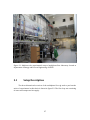
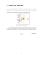
Figure 3.1: Medium scale experimental setup of multiphase flow laboratory located at
departmentofEnergyandProcessEngineeringofNTNU
3.1
SetupDescription
Thethree‐dimensionaloverviewofthemultiphaseflowrigusedtoperformthe
seriesofexperimentsinthisthesisisshowninfigure3.2.Theflowloopwasconsisting
ofwaterandcompressedairsupply.
27
ut,NTNU(Lilleby200
03)
Figurre3.2:MulttiphaseTesstRigLayou
Figure 3.3 shows a schematic overview of the exp
perimental setup witth more
oragewateerandpresssurized
details..Thewholesystemissplacedatttwolevelss.Largesto
air tan
nks (T1 an
nd T2) and
d water pu
ump (P1) were placed at baseement. Flow lines
continu
uedtolab‐llevelandaallflowmetters,contro
olvalves,h
horizontalttestsection
nandS‐
riserw
wereplaced
datthislev
vel.Theflo
owlineofttestwithin
nnerdiameeterof50m
mmwas
connecctedtoamixer/inletssectioncon
ntainingtheair/wateersupplyan
ndthemulltiphase
flow w
was forced up the S‐rriser. The air
a buffer tank (T3) was installled upstreeam the
mixing point to increase th
he air volum
me and em
mulate a long pipeline. The air volume
shouldbelargeen
noughtofo
orcetheliqu
uiduptheriserandcausesluggiingtooccu
ur.
A
Asoneoftthemostim
mportanteq
quipment, chokevalv
ve(V)was mountedaattopof
the S‐riser. It was used as the
t control actuator for controlling the in
nlet pressu
ure/ top
pressurreandoutlletflowden
nsityastheecontrolvaariables.Itwasalsopossibletoaadjustit
manuallly while running thee system in
n open‐loop
p position. Pressure transmitters (PT1
andPT
T2)andtheeconductan
nceprobeaasthedenssitymeter (C)werein
nstalledat various
placesiinthesetup
p,andwereeusedtoco
onstructanumberofdifferentccontrolstru
uctures.
A
After the S‐riser,
S
air and waterr were enttered into an overflow
w tank (T4
4), then
movedintoasmaallseparato
or(T5)thro
oughalarggeflexiblep
pipemadeo
ofhoses,an
ndwere
separatted there. The waterr is then reeturned fro
om the tesst section back
b
to thee water
largesttoragetank
kinthebassement.Theeairisventedoutwitthoutfurth
hertreatmeent.
Thedimen
nsionsoftheexperimeentalsetup
pareillustratedinfigu
ure3.4.Theelength
scaleissgiveninm
meters.
28
Figure3.3:MediumscaleTestRigLayoutwithmoredetails,NTNU
Figure3.4:ConfigurationoftheS‐shapedrisertestsection(Lilleby2003)
29
3.2
Equipment
Inthissectionpropertiesandpurposeofthemainequipmentaregiven.Allthe
pipes,bendsandotherconnectionsaremadeofacid‐proofsteel,AISI316L.Thisisthe
casefortheentirepipinguptothetestsections.Thevalvesaremadeoftreatedbrass,
andarequiteresistanttocorrosion.
3.2.1
Mainwaterstoragetank
Water is filled in a separator (T1). It is a 3 m 3 acid proof tank placed in the
basement.Fromtheseparator,waterispumpedthroughtheinfrastructure,intothetest
sectionandreturnedtotheseparatoragain.
Figure3.5:Mainwaterstoragetanklocatedinbasement
30
3.2.2
Airreservoirtank
Theairsupply(T2)isconnectedtothecentralhigh‐pressuresupply.Thissupply
is a pressure vessel made by Nessco and gives a pressure of 6‐7 bars, which is then
reduced through a pressure reduction valve to the operational pressure of (usually)
approximately3bars.
Figure3.6:Airreservoirtanklocatedinbasement
31
3.2.3
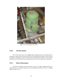
Airbuffertank
Theairbuffertank(T3)withavolumeof200litersandthetype“DN50flange”
has been made by the company “Laguna”. It is installed before the mixing point. To
make slugging possible, a large pipe volume for pressure buildup is necessary. The
buffertankisusedtoemulatethislargepipevolume.Themaximumpressurethebuffer
tankcanwithstandislimited.Forsafety,thetankhasbeenequippedwithasafetyvalve,
toensurethatthepressurenotwillexceed3Bars.
Figure3.7:Airbuffertank
32
3.2.4
Overflowtank
An overflow system is made to achieve pressure dependent liquid flow. It is a
ventedsteeltank(T4)filledwithwater.Flexiblepipesconnectthetanktotheseparator.
Abypassflowwillflowintothetankandbacktotheseparatorandmaintainaconstant
liquidlevelinsidethetank.Thepressureattheoverflowtankwillbeconstantequalto
the hydrostatic pressure of the liquid column from the tank. This will simulate a
constant reservoirpressure and make the inflow to the test section dependent onthe
inletpressure.Thesupply pipesfortheplasticoverflowtank aresmall,so itwillonly
workproperlyiftheflowthroughitisverylow.
Figure3.8:Overflowtankattopofriser
3.2.5
Pressuretransmitters
Pressure transducers (PT1 and PT2) made by Siemens were installed on the
buffer tank and riser to measure the buffer pressure and top pressure respectively.
Theyhaveaworkingrangeof0‐4bars.
33
3.2.6
Smallseparator
The flow from the overflow tank (T5) is moved into a small separator located
downthehosespipe.Apictureoftheseparatorisshownunderneathinfigure3.9.The
airfromtheriserisreleasedfromthetopoutlet.Thebottomoutletisusedforthewater
recycleandreturnsthewatertothewaterstoragetank.
Figure3.9:Smallseparator
3.2.7
Centrifugalwaterpump
A large centrifugal water pump (P1) of the type DN100 flange made by Wilo
Norge AS was used topush the water into the system. In order to prevent water flow
oscillationsthecentrifugalwaterpumpwasruninaveryhighlevelofpower(80%of
themaximum).Howevertogetthedesiredflowrateofwaterwhichwasnothigh(0.39
kg/sec)thewatercontrolvalvewasopeninsmallvalues,instead.
34
Figure3.10:Centrifugalwaterpump
3.2.8
Airflowmeter
The vortexflow meterof type DN40 wafer manufactured by JF Industrisensorer
wasusedtomeasuretheairflowrate(FIT1.01).Thenumberthatitgavewasintheunit
of Kg/hour and needed to be converted into the desired unit (kg/sec). It was located
upstreamtheairbuffertank.Theworkingrangeoftheairflowmeterwas5‐2180kg/h.
3.2.9
Waterflowmeter
The Electro‐magnetic water flow meter of type 1/2'' union, manufactured by JF
Industrisensorer was located upstream of the mixing point (FIT2.01). It has a working
rangeof0.19‐6.4 m 3 /h.
35
Figure3.11:Airflowmeter
Figure3.12:Waterflowmeter
36
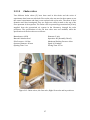
3.2.10
Chokevalves
Two different choke valves (V) have been used in this thesis and the series of
experimentshavebeenrunwithboth.Firstaslowvalvewasusedastheactuatortorun
the control experiments and then it was replaced with a fast valve. The effect of their
dynamics was then investigated. They are angle seat valves located on the top of the
riserupstreamoftheseparator.Thechokevalveisoperatedbypressurizedair(4bars)
supplied from the pressurized air system in the laboratory, through the valve
positioner. The specifications of the old slow valve were not available, while the
specificationsofthefastvalveareasfollows:
Manufacturer:ASCO
Diameter:2inch
Material:StainlessSteel Operation:NC(NormallyClosed)
PilotPressure:4‐10bar MaximumWorkingPressure:6bar
OperatorDiameter:90mm
Signal:4‐20mAmp
OpeningTime:2sec
ClosingTime:2.5sec
Figure3.13:Chokevalves;left:Fastvalve,Right:Slowvalveanditspositioner
37
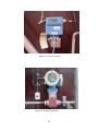
3.2.11
Conductanceprobe(C)
In the second series of experiments with the fast valve a cascade control
structurewasusedwithoutflowdensityandthetoppressureasthecontrolvariables.
Conductance probe was applied to measure the density of the outflow from the riser.
The probe has been calibrated by Kazemihatami (Kazemihatami 2012) very recently.
Theoutputoftheprobewasintheformofvoltage.Thecalibrationcurvepresentedby
Kazemihatamiwasusedtofindtherelationbetweenvoltageandholdup.Equation3.1
showsthisrelation.HmeansholdupandVmeansvoltage.
H  0.9857V Equation3.1
Thedensityofmixedflowisfoundfromtheequation3.2:
 m   water . H   air . 1  H  Equation3.2
Afterinsertingtherelatedvaluesintheaboveequation,thedensityofmixedflow
isfoundasafunctionofvoltage:
 m  984.513V  1.204 Equation3.3
Figure3.14:Theconductanceprobe
38
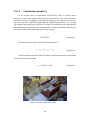
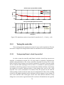
3.2.12
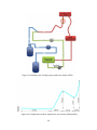
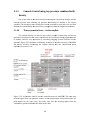
LabVIEW
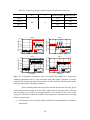
The Laboratory Virtual Instrumentation Engineering Workbench (LabVIEW)
softwaredevelopedbyNationalInstrumentswasusedforinstrumentationcontroland
data logging. The user interface is illustrated in figure 3.15. The pressures, flow rates
and valve position could be monitored directly from the interface. In addition it was
possible to run the loop manually by manipulating choke valve opening, or
automatically by setting tuning parameters for PID/PI/P controllers. Some
modificationswereappliedincaseofcontrol.Twomodesofcontrolwereimplemented
in the program; a single mode and a cascade mode. The single mode used buffer
pressureascontrolvariableandthecascademodewasusingtoppressureandoutflow
densityascontrolvariables.Aschematicviewofcontrolmodesarepresentedinfigure
3.16.
Figure3.15:LabVIEWuserinterface
39
Figure3.16:ImplementedcontrolmodesinLabVIEW
40
4 Simulationofexperimentalcases
4.1
OLGA®,multiphasesimulationtool
OLGA® (OiL and GAs simulator) is a commercial multiphase flow simulator
widelyusedintheoilandgasindustry.Itsolvesmanynumericalequationstosimulate
theflowbyconsideringthesystemdynamicsandoffersheatandmasstransfermodels.
TheexperimentalcasewasconstructedinOLGA.Thedesignedcontrollerswith
differenttuningstrategieswereusedandtheresultswerecompared.Inordertofitthe
OLGAmodelwiththeMATLABmodelsandexperimentssomeoftheparameterswere
manipulatedwithinlimitedranges.OLGA®version7.1wasusedforthesimulations.
In this chapter the case construction with implementing the S‐shaped riser
geometry, fluid properties, numerical settings and boundary conditions is explained
stepwise.
4.2
Constructionofthecase
Establishment of a good case with appropriate particular items such as fluid
properties,numericalsettings,initialandboundaryconditionsandflowpathgeometry,
wastheinitialstepforsimulationprocess.The“S‐risersimple”casemadebyJahanshahi
(Jahanshahi and Skogestad 2011) was basically used for the open‐loop simulations.
Some improvements and modifications were applied after the file was received. For
open‐loop simulations the modifications were in terms of numeric and for theclosed‐
loopsimulationstheywererelatedtoimplementingthePIDcontrollerintothecase.In
termsofnumericsomeIntegrationparametersweremanipulatedinPropertieswindow
oftheprogram.
41
4.2.1
Flowpathgeometry
The “S‐riser simple case” with a geometry based on the experimental set‐up at
the Department of Energy and Process Engineering was used. The reason to use such
geometry is that the simulation results are to be compared with the experimental
resultsinthethesis.Theexactgeometryispresentedintable4.1.
The X‐Y coordinates have been calculated with respect to table 4.1and the
resultinggeometryhasanoverviewofthefigure4.1.
Accordingtotheexperimentalsetupinmultiphaseflowlaboratory,thesources
ofairandwaterareplacedinthebeginningandtheendofthebuffertankrespectively.
Table4.1:ThegeometryoftheS‐riserexperimentalset‐up
Pipe
L[m]
D[m]
 [ ] out  in  1
8.125
0.20
‐45.0
2
3.000
0.05
‐10
3
6.050
0.05
‐4.0
4
1.200
0.05
‐1.8
5
1.106
0.05
‐1.8
‐61.8
6
4.110
0.05
61.8
7
0.709
0.05
61.8
‐32.0
8
2.160 0.05
‐32
9
1.716
0.05
‐32
79.0
10
1.820 0.05
79.0
11
1.150
0.05
90
42
S‐risergeometry
7
6
5
y[m]
4
3
2
1
0
‐1
‐5
0
5
x[m]
10
Figure4.1:GeometryofS‐riserinOLGA
15
4.2.2
Fluidproperties
AllfluidpropertieshadbeenwritteninPVTfileby(JahanshahiandNilsen2012).
Itisatableofphasecompositionsatdifferenttemperaturesandpressuresandismade
by a program called PVT‐Sim. By specifying temperature and pressure limits and the
compositions of the fluids involved, the program calculates the values for the phase
compositions.Heattransferandtemperaturechangewerenotimportantinsimulations
due to experimental condition. Water was assumed as an incompressible flow. Heat
transfer and temperature related properties such as enthalpy or entropy were filled
withdummynumbers.
4.2.3
Boundaryandinitialconditions
Thetypesoftheairandwatersourcesasinletnodsweredefinedasinletmass
flow. The flow rates were fixed for all simulations. The volume fractions were
establishedto1forbothnodessinceonlywaterorairwasinjectingthroughthenode.
The outlet nod type was selected to pressure type and it has been set to atmospheric
pressure.
43
4.2.4
Numericalsetting
Thenumericalsettingspecificationssuchassimulationtimeandtimestepwere
adjusted in different numbers from case to case. This is due to the diversity of phase
velocityindifferentcases.
4.3
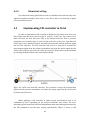
ImplementingPIDcontrollerinOLGA
InordertoimplementaPIDcontrollerinOLGAfirstapositivecheckvalvewas
placedright afterthe water source in pipe2, section 1 of the case. The reason wasto
make sure that the flow will move only in the defined direction. Then a pressure
transmitterwaslocatedinpipe2,section2thatistheinletoftheriser,rightafterthe
buffertank.Itwasaimedtomeasurethebufferpressureandsendthepressuresignal
into the PID controller. The PID controller was used in a way that it received the
measurementsignalfromthepressuretransmitterandsenttheoutputsignalintothe
chokevalvelocatedattopoftheriser(Pipe8,section3).Chokevalvescanbesimulated
byselectingtheHydrovalveforthevalvemodelinOLGA.
Figure 4.2: OLGA case with PID controller. The controller receives the measurement
signal from thepressure transmitter and sends the output signal into the choke valve
locatedattopoftheriser.
When applying a PID controller in OLGA several specifications need to be
established by user, depending on the desired conditions and results. The more
importantspecificationsthathavebeenmanipulatedmanytimesduringsimulationsare
the PID parameters and the time varying specifications. When it comes to PID
44
parametersinpropertywindowofthesimulator,AMPLIFICATIONreferstothegainof
thecontroller;BIASisthedesiredinitialoutputvalue(itwasusedasthedesiredvalve
openinginoursimulations);DERIVATIVECONSTisthetimeconstantforthederivative
action and INTEGRALCONST is the time constant for the integral action. As the time
varying specifications the MODE was set to AUTOMATIC and the SET‐POINT values
werechangedfromonesimulationtoanother.
45
5 Resultsanddiscussion
The purpose of this chapter is to present the results from experiments and
simulationsandaclearcomparisonofthem.Theexperimentalresultsfromtwoseries
ofexperimentsusingaslowandafastchokevalvewillbepresentedinsection5.1.The
effort of cascade control experiment using top pressure combined with density as
measurements and the faced issues has been also mentioned there. Section 5.2
evaluatestheeffectofcontrolvalvedynamicsthroughcomparingresultsofslowvalve
withthoseoffastvalve.Thesimulatedresultswillbeexplainedinsection5.3.Insection
5.4 the experimental results are compared with simulated results. In section 5.5 the
threedifferentusedtuningmethodshavebeencomparedandthebesttuningmethod
hasbeeninvestigated.
5.1
Experimentalresults
The operating procedures and the results from experimental activities done at
NTNUmultiphaseflowlaboratoryarediscussedinthissection.
Foreachseriesofexperimentswithvalve1(slowvalve)orvalve2(fastvalve)
the open‐loop system with basic conditions would be explained first. Then the
procedureofimplementingclosed‐loopsteptestandcalculatingthetuningparameters
byusingdifferenttuningmethodswillbediscussed.Theresultsoftuningintheformof
tuningrulesareexplainedthereafter.Finallytheclosed‐loopresponsesusingcalculated
tuningparameterswillbepresentedasthemainresultsoftheexperimentalwork.
46
5.1.1
Seriesofexperimentswithvalve1(slowchoke
valve)
Theexperimentalworkinthisthesisstartedwithusingslowchokevalveasthe
actuator.Thegoalwas torepeatthe sameseriesoftestswithaslow andafastchoke
valveandthenevaluatetheeffectofcontroldynamicsonthefinalresults.
5.1.1.1
Open‐loopexperiments
Thestartingpointintheexperimentswasrunningtheloopinmanualmode.The
testswererunindifferentvalveopeningswithfixedliquidandgasflowrateswhileno
controllerwasimplementedinthesystem.Itwasaimedtopresentthesystembehavior
innaturalconditionswithoutcontrol.Theinflowconditionsandtherelatedbifurcation
diagramarepresentedbelow.
5.1.1.1.1 Inflowconditions
The applied fixed flow rates have been wl  0.3927 [kg / sec ] for water and
wg  0.0024 [ kg / sec ] for air (See figure 5.1.) These flow rates correspond to U sl  0.2
[m / sec] and Usg  1 [m / sec] astheliquidandgassuperficialvelocities.Thewaterflow
rate could be set in lab view by adjusting the pump frequency and the control valve,
whiletheairflowrateneededtobesetwithamanualvalveinthepathoftheflow.The
reasonwasthatthecontrolvalvefortheairwasbroken.Themanualvalvewasfarfrom
thescreenandthismadeitdifficulttoobtaintheexactflowrate.
The water flow rate was not also easy to set. Large variations in the flow rate
were eliminated by running the pump with a high frequency and opening the control
valve in a small value. The more opening the choke valve, the more slugging the flow
regime and the more unstable the flow rates were resulted. In the following series of
experiments,aconstantflowrateofairandwaterwasused.Asaresult,thewaterand
air flow rates needed to be readjusted when the valve opening in open‐loop was
changed.However,whenusingacontrollerinclosed‐loopmode,itwasconsiderednot
to be reasonable to readjust the inflow conditions. Figure 5.1 compares variations of
flowratesandpressureintwodifferentvalveopenings.
47
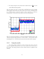
‐3
Basisconditionwith20%valveopening
AirFlowrate[kg/sec]
x10
2.4
2.2
2
0
100
200
300
400
WaterFlowrate[kg/sec]
0.38
0.36
0.34
0.32
0
100
200
300
400
200
198
196
194
192
190
0
100
200
time[sec]
300
2.6
x10
400
Basisconditionwith100%valveopening
2.4
2.2
2
0
50
100
150
200
250
300
350
50
100
150
200
250
300
350
50
100
150
200
time[sec]
250
300
350
0.5
0.45
0.4
0.35
0
BufferPressure[kPa]
BufferPressure[kPa]
WaterFlowrate[kg/sec]
AirFlowrate[kg/sec]
‐3
2.6
200
180
160
140
120
100
0
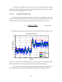
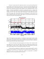
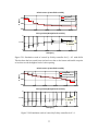
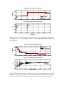
Figure5.1:Illustrationofbasisopen‐loopconditionsincaseofflowratesandpressure.
The left series of plots are illustrating the system with valve opening Z=0.2 that is
related to the stable region while the right side plots present the system with valve
openingZ=1thatisrelatedtotheunstableregion.Largeoscillationsareclearsignsof
instabilityatZ=1.
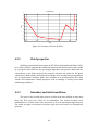
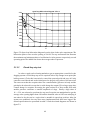
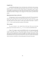
5.1.1.1.2 Bifurcationdiagram
The experiments were started with the valve opening of Z=0.2. Then the valve
was open stepwise until it was fully open. The results of buffer pressure were logged
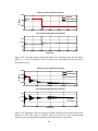
and the related bifurcation diagram was plotted, presented in Figure 5.2. The critical
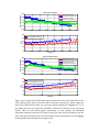
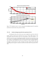
stabilitypoint(thebifurcationpoint)isthemaximumchokevalveopeningthesystem
canhavewhilebeingstable.Inthepresentedbifurcationdiagram,thetoplinetracksthe
maximum values of pressure at each operating point, the bottom line presents the
minimumvaluesofpressureandthemiddlelineshowstheaveragevaluesofthebuffer
pressureatdifferentvalveopenings.Asclearinthefigurethecriticalstabilitypointwas
foundtobeatapproximately26%chokevalveopening(Z=0.26).
48
OpenloopBifurcationDiagram‐Valve1
210
200
InletPressure[Kpa]
190
180
170
160
150
140
130
120
110
0.2
0.3
0.4
0.5
0.6
Z
0.7
0.8
0.9
1
Figure5.2:Open‐loopbifurcationdiagramfromtheslowchokevalveexperiments.The
bifurcationpointoccursatvalveopeningofZ=0.26.Thetopandbottomlineillustrate
themaximumandminimumvaluesofoscillationsforinletpressurerespectivelyateach
operatingpoint.Themiddlelineshowstheaveragevaluesofpressure.
5.1.1.2
Closed‐loopsteptest
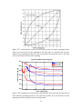
Inordertoapplyeachoftuningmethodstogetanappropriatecontrollerforthe
sluggingsystemaclosed‐loopsteptestisrequiredwithastepchangeinset‐point(the
bufferpressure).Todothisitwastriedtocontrolthesystembytrialanderror.AP‐only
controllerwasselectedandastheinitialguessforthegain,abigvalueof100wastried.
Thereasonwasthattheset‐pointvaluewasasmallnumber(pressureinbars)andthe
gainhadtobeselectedinawaythatitcouldchangetheoutput(Z)inalargerangeafter
a small change in set‐point. Increasing the gain resulted in a more stable flow with
smaller pressure variations or smaller amplitude of slugs. Finally a high value of
K c 0  220 wasselectedtoperformthesteptest.Set‐pointwasmanipulatedtogetthe
averagevalveopeninghigherthan0.26andtheobtainedvalueof0.29wassatisfying.It
was aimed to do the test in a region that is unstable in open‐loop position. After the
system was stabilized, four step tests were implemented and data were logged. The
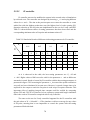
relatedspecificationsarepresentedintable5.1andtherelateddiagramsareshownin
figure5.3.
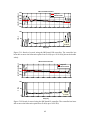
49
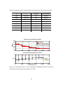
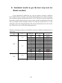
Table5.1:Closed‐loopsteptestspecificationsrunwithslowchokevalve
I Kc0 Initialset‐point
Finalset‐point
1.52
1.72
1.73
1.54
1.54
1.73
1.49
1.70
Test_1
Test_2

220
Test_3
Test_4
Test‐1
1.65
1.6
Setpoint
Data
1.55
1.5 0
100
200
1.7
1.65
1.6
Setpoint
Data
1.55
1.5 0
200
400
time[sec]
1.6
1.4
Setpoint
Data
200
600
1.7
1.6
Setpoint
Data
1.5
0
600
400
Test‐4
1.8
1.8
0
300
Test‐3
1.75
Inletpressure[bar]
Inletpressure[bar]
1.7
Test‐2
2
Inletpressure[bar]
Inletpressure[bar]
1.75
200
400
600
time[sec]
800
Figure 5.3: Presentation of different tests of set‐point step change for a closed‐loop
feedback experiment with a P_only controller using inlet (buffer) pressure as control
variable.Test‐4showsthebestcharacteristicsincaseofdesiredovershootandsteady
stategainrequiredfortuningthecontroller. Afterevaluatingdatafromsteptestsitseemedthatthelastone(test_4)has
bettercharacteristicscomparedtotheotherswithrespecttothepointthataunitstep
test was going to be used for all tuning methods. It was decided to use test_4 in the
tuning of controller by different methods. Some important considerations in selecting
thebeststeptestwere:
1. ForthesteptesttobeusedinShams’smethodtherecommended0.3overshoot
wasdesired.
50
2. The steady state gain of the system must be smaller than one (
y
 1 ) to be
ys
usedinIMC‐basedtuningmethod.
Since the response was noisy, a low‐pass filter in MATLAB from the type of Simple
infiniteimpulseresponsefilterwasusedtoreducethenoiseeffect.Asmoothingfactor
of   0.001 was used to smooth the signal as well as required (   1 means no
filtering).Figure5.4illustratesthestepresponseusedinthetuningmethods.
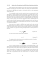
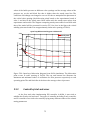
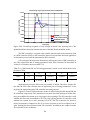
175
InletPressure[Kpa]
170
165
160
155
Setpoint
Data
Filtered
150
145 0
100
200
300
400
500
time(sec)
600
700
800
900
Figure 5.4:Set‐pointstep changefor aclosed‐loopfeedback experiment withaP_only
controller using inlet (buffer) pressure as control variable. A low pass filter with a
smoothingfactorof   0.001 wasusedtoremovethenoiseeffectfromtheresponse.
5.1.1.3
Tuningthecontroller
The tuning methods explained in section 2.9 have been used to tune the
controllerusingbuffer(inlet)pressureasthecontrolvariableandslowchokevalveas
the actuator. The tuning procedure and the related results are explained in the
following.
51
5.1.1.3.1 TuningbyShams’sclosed‐loopmethod
The first method to be used for tuning of the controller was Shams’s method
developed by Shamsuzzoha (Shamsuzzoha and Skogestad 2010). In order to tune by
Shams’smethod,explainedinsection2.9.1theinformationfromthesteptestexplained
inprevioussection(Seefigure5.4)wereused.Then,theovershootwascalculatedand
the appropriate tuning parameters were found. Table 5.2 shows the resulted tuning
parameters by Shams’s method. Kc0 is the initial gain used in the step test, Kc is the
calculated proportional gain, and  I is the integral tuning parameter. The system has
beenconsideredasafirstorderplusdelaymodel.
Table5.2:TuningparametersfromSham’smethodforthesluggingsystem
Kc0 Z ave Overshoot
Offset
Kc I 220
0.29
0.3846
0.6501
121.5189
224.3679
Itwastriedtocontrolthesystembytherelatedtuningparametersseenintable
5.2.Yet,thementionedtuningparameterscouldn’twork;meaningthatthePIcontroller
withtheseparameterswasnotabletostabilizethesystemandseveresluggingwasnot
eliminated.WemaysaythattheSham’stuningmethodisnotasuitableapproachfor
thesluggingsystem.
5.1.1.3.2 TuningbasedonIMCdesign
Next method applied in tuning of controller in experiments was the IMC‐based
tuning described in section 2.9.2. To do this, it was tried to identify the closed‐loop
stable system with respect to the data from step test and according to the method
proposedbyJahanshahi(JahanshahiandSkogestad2013)explainedinsection2.9.2.1.
Theidentifiedmodelofclosed‐loopsystemwasintheformof:
Gcl ( s) 
11.74 S + 0.606
96.38S 2  10.88S  1
Equation5.1
Theidentifiedclosed‐looptransferfunctionisshownbytheblacklineinfigure5.5.
52
Closed‐loopstepresponse
175
Inletpressure[kPa]
170
165
160
155
set‐point
Exp.data
Filtered
identified
150
145 250
300
350
400
450
500
time(sec)
550
600
650
700
Figure5.5:Presentationofidentifiedclosed‐loopstepresponse.Thedashedblackline
showstheidentifiedclosed‐looptransferfunctionobtainedfromIMCdesign.
Then, the open‐loop unstable system has been back calculated by using the
procedure proposed by Jahanshahi (Jahanshahi and Skogestad 2013). The open‐loop
unstablesystemhastheformof:
-0.0005538 S - 2.858e-05
P ( s)  2
S  0.008984S  0.004088
Equation5.2
ThentheIMCcontroller(C)isdesignedbyusingthemethodexplainedinsection
2.9.2.2. The time constant of the closed‐loop system is an important manipulated
parameterandhasbeenselectedas   20 .Thisnumberwasobtainedbytrialanderror
andexperiencingdifferentresults.ThedesignedIMCcontrolleris:
C ( s) 
287.0673( S  0.02146S  0.0007862)
S(S+0.05161)
2
Equation5.3
The IMC controller is a second order transfer function which can be written in
form of a PIDF controller. PIDF is a PID controller which a low‐pass filter has been
appliedonitsderivativeaction.ItwillbementionedasPIDcontroller.
53
APIcontrollerwasalsoobtainedbyreducingtheorderofIMCcontrollerto1.
Therelatedtuningparametershavebeenobtainedandareshownintable5.3.
Table5.3:IMC‐basedPIDandPItuningparameter
Kc0 Kc I D F PID 220
34.6387
7.92
141.2113
19.3773
PI 220
287.0673
65.6371
_
_
Theapproachofimplementingthelowpassfilterintheexperimentsisdescribed
inappendixA.
To find the control results all related tuning parameters were implemented in
LabVIEW and the loop was run in the stable region with an average valve opening of
Z=25%.Thenitwastriedtodecreasetheset‐pointvalueinastepwisemanner.Ateach
stepitwaswaiteduntilthesteadystatewasreachedandthenanewstepofreduction
was done. Figures 5.6and 5.7 describe the results of control using the IMC‐based PID
andPIcontrollersrespectively.Theexperimentalsluggingsystemcouldbestabilizedup
to Z= 40% with IMC‐based PID controller and up to Z= 38.4% with IMC‐based PI
controllereventhoughthecontrollershavebeendesignedatvalveopeningofZ=28%.
54
InletPressure[Kpa]
IMCbasedPIDController
190
Setpoint
Measurement
180
170
160
150
140 0
200
400
600
800
1000
1200
X:1363
Y:40.2
50
40
Z[%]
1400
30
20
10
0
0
200
400
600
800
time[sec]
1000
1200
1400
Figure5.6:ResultofcontrolusingtheIMC‐basedPIDcontroller.Thecontrollerhasbeen
abletomovethebifurcationpointfromZ=26%uptoZ=40.2%.
InletPressure[Kpa]
IMCbasedPIController
190
Setpoint
Measurement
180
170
160
150
140 0
200
400
600
800
1000
1200
50
Z[%]
40
X:1266
Y:38.39
30
20
10
0
0
200
400
600
800
time[sec]
1000
1200
1400
Figure5.7:ResultofcontrolusingtheIMC‐basedPIcontroller.Thecontrollerhasbeen
abletomovethebifurcationpointfromZ=26%uptoZ=38.39%.
55
5.1.1.4
Inconclusiveeffortsandtherelatedpracticalissues
Whenworkingwiththefirstvalve,someeffortswereinconclusiveandnoresults
wereproduced.Belowsomeexplanationsaregiven.
5.1.1.4.1 TuningthecontrollerbySimpleonlinemethodbasedonidentified
MATLABmodelofthesystem
AsthelastmethodoftuningitwastriedtousesimplePItuningrulesdescribed
in section 2.9.3. The method has been proposed by Jahanshahi (Jahanshahi and
Skogestad2013)andisbasedontheidentifiedMATLABstaticmodelofthesystem.To
implement this method, first the simple static MATLAB model of the system which
tuningrulesarebasedonneededtobemodifiedandfittotheexperimentalsteadystate
model. For a reasonable result, it was required to have an accurate model of the
experiments. Though, right in that time the lab technician replaced the current valve
withthefastvalvesincehewasgoingtovacationandthiscouldn’tbedoneforalong
time.Thereforethistuningmethodwastriedonlybythesecondvalve.
5.1.1.4.2 Applyingtimedelayinthecontroller
Oneimportantissueregardingtheslowvalveteststhatneedstobementionedis
about applying time delay. It was aimed to check the robustness of control system by
implementing delay on measurement. In order to do this, an algorithm was
implementedinLabVIEWbyoneofthelabtechnicians.Itwasadigitaldelaylinewhich
delayed the samples of the measured data by a desired given time. The desired delay
timecouldbesetfromthefrontpanel.Yetthedelaysettingcouldn’tworkinadesired
way, meaning that even for very small values of delay the system switched to severe
sluggingandthecontrolwasimpossible.Itwasclearthatforsuchalongpipelineriser
systemsmallvaluesofdelayintherangeofmillisecondscouldn’tcrashthecontroland
thereasonofinconveniencymaybefromLabVIEW.Itmightbebecauseofmistakesin
the algorithm or in the connections inside LabVIEW. Since the system was inmedium
scaleandnooneelseexceptforthelabtechnicianswasabletodomodificationsinthe
systemorLabVIEWandalsoduetotimeissuesitwasdecidedtoignoreimplementing
timedelayaftercounselingwithmysupervisor.Itwasanextraworktobedoneinthe
thesiswhilethenextrequiredexperimentswerenotstartedyetatthattime.
56
5.1.2
Seriesofexperimentswithvalve2(fastchoke
valve)
Thenextseriesofexperimentalworkinthisthesiswasrepeatingthefirstseries
of tests with a new fast valve as the actuator. A new method of tuning has been used
hereinadditiontothetuningmethodsofprevioussection.
5.1.2.1
Open‐loopexperiments
Theloopwasrunin manualmodewithfixedflowratesof wl  0.3927 [kg / sec ] forwaterand wg  0.0024 [kg / sec ] forair.Theseflowratesarethesamevaluesusedfor
the slow valve. The related inflow conditions have been fully described in section
5.1.1.1. The tests were run in different valve openings with fixed liquid and gas flow
rates without applying control. The system behavior in natural conditions was then
presentedwiththerelatedbifurcationdiagramasseeninfigure5.8.
5.1.2.1.1 Bifurcationdiagram
The starting point was the valve opening of Z=0.1. Then the valve was open
stepwiseuntilitwasfullyopen.Theresultsofbuffer(inlet)pressurewereloggedand
therelatedbifurcationdiagramwasplotted.Thecriticalstabilitypoint(thebifurcation
point)isthemaximumchokevalveopeningthesystemcanhavewhilebeingstableand
islocatedatZ=0.16forthesystemwithvalve2.Inthepresentedbifurcationdiagram,
thetoplinetracksthemaximumvaluesofpressureateachoperatingpoint,thebottom
line presents the minimum values of pressure and the middle line shows the average
values of the buffer pressure at different valve openings. Small pressure oscillations
before the bifurcation point are due to hydrodynamic slugs and are not the signs of
instabilities.
57
OpenloopBifurcationDiagram‐Valve2
220
InletPressure[Kpa]
200
180
160
140
120
0.1
0.2
0.3
0.4
0.5
Z
0.6
0.7
0.8
0.9
Figure 5.8:Open‐loopbifurcation diagramfromthefastchokevalveexperiments.The
bifurcationpointoccursatvalveopeningofZ=0.16.Thetopandbottomlineillustrate
the maximum and minimum values of inlet pressure respectively at each operating
point.Themiddlelineshowstheaveragevaluesofpressure.
5.1.2.2
Closed‐loopsteptest
Justliketheexperimentserieswithvalve1,thefirststeptotunethecontroller
withanytuningmethodwasaclosed‐loopsteptestwithastepchangeinset‐point(the
buffer pressure). The loop was closed with a P‐only controller with a gain value of
K c 0  250 .Thestepchangewasdoneinaregionthatisunstableinopen‐loopposition.
The average of valve opening was Z  0.18 . The related plot is shown in figure 5.10.
Since the response was noisy, a low‐pass filter in MATLAB from the type of Simple
infiniteimpulseresponsefilterwasusedtoreducethenoiseeffect.Asmoothingfactor
of   0.25 wasusedtosmooththesignalaswellasrequired(   1 meansnofiltering).
58
166
164
InletPressure[Kpa]
162
160
158
156
154
152
Setpoint
Measurement
Filtered
150
148 0
100
200
300
time(sec)
400
500
600
Figure 5.9:Set‐pointstep changefor aclosed‐loopfeedback experiment withaP_only
controller using inlet (buffer) pressure as control variable. A low pass filter with a
smoothingfactorof   0.25 wasusedtoremovethenoiseeffectfromtheresponse.
5.1.2.3
Tuningthecontroller
Three different methods explained in section 2.9 have been used to tune the
controller using buffer (inlet) pressure as the control variable and fast choke valve as
theactuator.Thetuningprocedureandtherelatedresultswillbepresentedbelow.
5.1.2.3.1 TuningbyShams’sclosed‐loopmethod
Shams’s tuning method developed by Shamsuzzoha (Shamsuzzoha and
Skogestad 2010) was used as the first tuning method. Table 5.4 shows the resulted
tuningparametersbyShams’smethod.Thesystemhasbeenconsideredasafirstorder
plus delay model. The information from the closed‐loop step test (See figure 5.9) was
usedtofindthetuningparameters.
Table5.4:TuningparametersfromSham’smethodforthesluggingsystem
Kc0 Z ave Overshoot
Offset
Kc I 250
0.18
1.5738
1.3823
331.0775
246.7640
59
Asexpected,accordingto resultsof valve1,thePIcontroller withthesetuning
parameterscouldn’tstabilizethesystem,meaningthatShams’smethodisnotasuitable
methodtotunethesluggingsystemcontroller.
5.1.2.3.2 TuningbasedonIMCdesign
IMC‐based tuning method described in section 2.9.2 was applied as the next
methodtotunethesystemwithfastvalve.Datafromsteptest(Seefigure5.9)wereused
andThemodelofclosed‐loopsystemwasidentifiedasexplainedinsection2.9.2.1.
Gcl ( s ) 
9.076 S + 0.7406
64.76S 2  4.635S  1
Equation5.4
Theidentifiedclosed‐looptransferfunctionisshownbytheblacklineinfigure5.10.
Closed‐loopstepresponse
166
164
InletPressure[Kpa]
162
160
158
156
154
152
set‐point
Measurement
Filtered
identified
150
148 0
100
200
300
time(sec)
400
500
600
Figure5.10:Presentationofidentifiedclosed‐loopstepresponse.Thedashedblackline
showstheidentifiedclosed‐looptransferfunctionobtainedfromIMCdesign.
Theopen‐loopunstablesystemwasthencalculatedastheformofequation5.5
byusingtheprocedureproposedbyJahanshahi(JahanshahiandSkogestad2013).
60
-0.0005606 S - 4.574e-05
P ( s )  2
S  0.06858S  0.004006
Equation5.5
TheIMCcontroller(C)wasobtainedthenastheequation5.6(Seesection2.9.2.2).
Avalueof   24.5 wasusedforthetimeconstantoftheclosed‐loopsystem.Thisvalue
wasmanipulatedbytrialanderroruntilasatisfyinggain,phaseanddelaymarginwas
obtainedforthecontroller.
C
340.7491( S  0.005194S  0.000356)
S ( S  0.0816)
2
Equation5.6
TheIMCcontrollerasasecondordertransferfunctionwasthenwritteninform
ofaPIDcontrollerwithalow‐passfilterappliedonitsderivativeaction(Wemaysaya
PIDFcontroller).
APIcontrollerwasalsoobtainedbyreducingtheorderofIMCcontrollerto1.
Therelatedtuningrulesareshownintable5.5.
Table5.5:IMC‐basedPIDandPItuningparameters
Kc0 Kc I D F PIDF 250
3.4736
2.3368
1189.9378
12.2552
PI 250
340.7491
229.2276
_
_
Thefunction“PIDAdvancedVI”fromLabVIEWwasusedtoimplementthelow‐
passfilterintheexperiments(seeappendixA).
ThePIDtuningparameterswereimplementedinLabVIEW.Firstthesystemwas
runinopen‐loopmannerwithamanualvalveopeningofZ=0.2anddatawerelogged.
Then the loop was closed with a set‐point P=170 kPa that results in an average valve
openingofZ=0.16.Aftercoupleofminutesitwastriedtodecreasetheset‐pointvaluein
a stepwisemanner. At each step it was waited until the steady state was reached and
then a new step of reduction was applied. The same was done with PI tuning
parameters.Figures5.11and5.12describetheresultsofcontrolusingthe IMC‐based
PID and PI controllers respectively. The experimental slugging system could be
stabilizeduptoZ=0.30withIMC‐basedPIDcontrolleranduptoZ=0.29withIMC‐based
PIcontroller.
61
InletPressure[Kpa]
IMCbasedPIDController
220
Setpoint
Measurement
200
180
160
140
120 0
200
400
600
800
1000 1200 1400 1600 1800 2000
Z[%]
100
50
0
0
X:1810
Y:30.19
200
400
600
800
1000 1200 1400 1600 1800 2000
time[sec]
Figure 5.11: Result of control using the IMC‐based PID controller. The controller has
beenabletomovethebifurcationpointfromZ=16%uptoZ=30.19%(aboutthedouble
value).
InletPressure[Kpa]
IMCbasedPIController
Setpoint
Measurement
200
180
160
140
0
200
400
600
800
1000
1200
1400
1600
1800
1400
X:1526
Y:29.35
1600
1800
Z[%]
100
50
0
0
200
400
600
800
1000
time[sec]
1200
Figure5.12:ResultofcontrolusingtheIMC‐basedPIcontroller.Thecontrollerhasbeen
abletomovethebifurcationpointfromZ=16%uptoZ=29.35%.
62
5.1.2.3.3 SimpleonlinePItuningbasedonMATLABmodelwithgainscheduling
SimplePItuningrulesdescribedinsection2.9.3wasusedasthelastmethodof
tuningthecontroller.SincethemethodisbasedonthesimplestaticMATLABmodelof
the system, the MATLAB model needed to be identified and fit to the experimental
steadystatemodel.
For a reasonable result, it was first required to have an accurate model of the
experiments.TofindthemodeltheloopwasclosedwithaPIcontrollerandwasrunin
the region after stability point in open‐loop bifurcation diagram. This was done such
thatset‐pointwassettoavaluelowerthanthecorrespondingvalueofthebifurcation
point, then it was waited until steady state was reached and data were logged. The
average of valve opening was found from logged data and the obtained point was
located on the steady state experimental model. By repeating this for some other set‐
pointvaluesthesteadystatelineofexperimentalmodelwasfound.Itisshowninfigure
5.13withtheblackmidline.
Next step was to modify the MATLAB static model and fit that with the
experimentalmodel.Asdescribedinsection2.9.3.1theMATLABmodelisderivedbased
onthevalveequationandisafunctionofvalveopening.Thereforeagoodassumption
ofvalveequationisveryimportantinusingthesimplemodel.Thevalveequationisas
theform:
w  K pc f ( z) p Equation5.7
Thevalveislinearanditscharacteristicisdefinedas:
f ( z)  Z Equation5.8
Thesimplemodelfortheinletpressureisasdefinedinsection2.9.3.1andthe
staticgainofthesystembecomesinformof:
k ( z) 
2w2
 . z 3.K pc 2
Equation5.9
Since the tuning parameters are found based on this MATLAB model, a good
matchbetweenthismodelandtheexperimentalmodelisveryimportantmeaningthat
thevaluesofinletpressureandthestaticgainobtainedbythemodelneededtobetrue
values. The parameters Lr (length of riser), P _ Vmin (minimum Pressure drop over the
valve) and K pc (the valve constant) were manipulated many times until the desired
match with the experimental model was reached. Below is a discussion of these
parameters.
63
Lengthofriser
InMATLABmodellengthofriserisdirectlyusedtocalculatethestaticpressure
oftheriserwhenitisfilledwithliquidandthereafterthisstaticpressureisusedtofind
theinletpressureatanylevelofvalveopening.Thereforemanipulatingofthatcouldbe
veryhelpfulinproducingdesiredresults.Theexactlengthofriserintheexperimental
setuphasbeen6.433m.Though,itwaschangedto6.7minmodeltoprovidethebest
results.
Minimumpressuredropoverthevalve
Thisparameterisusedinseveralcalculationsinthemodel.Themostimportant
oneisthevalueofinletpressureinthefullyopenpositionofthevalvethatuses P _ Vmin directly (See section 2.9.3.1). Level of the curve in the inlet pressure plot of the model
was quite affected by inlet pressure at fully open position of the valve. A value of
P _ Vmin  3kPa wasusedtogetthebestfitnessofthemodels.
Valveconstant
The valve constant K pc has a major effect on the slope of the curve in the inlet
pressureplotofthemodel.Avalueof K pc  1.6 103 wasusedintheMATLABmodel.
Figure 5.13 compares simple static MATLAB model to the experimental model.
As clear in the figure there is a good match between the two models. The MATLAB
modelisattachedinAppendixC.5.Theblackmidlineinthefigurepresentsthesteady
statevaluesoftheinletpressureandtheredmidlineisthevaluesofinletpressurefrom
theMATLABmodel.Thetopandbottomblacklinesshowthemaximumandminimum
valuesofpressureoscillationsateachoperatingpointintheopen‐loopsystem.
64
220
SimplestaticMATLABmodel
Experimental
InletPressure[kPa]
200
180
160
140
120
0.1
0.2
0.3
0.4
0.5
Z
0.6
0.7
0.8
0.9
Figure 5.13: Simple static MATLAB model compared to the experimental model. The
blackmidlineinthefigurepresentsthesteadystatevaluesoftheinletpressureandthe
redmidlineisthevaluesofinletpressurefromtheMATLABmodel.Thetopandbottom
black lines show the maximum and minimum values of pressure oscillations at each
operatingpointintheopen‐loopsystem.
In order to find the appropriate tuning parameters based on the identified
MATLABmodelaclosed‐looptestwithstepchangeofset‐pointisrequired(Seesection
2.9.3.2).Datafromthesteptestexplainedinsection5.1.2.2wasused(Seefigure5.9)and
theparameter  wasfoundfromtheequation2.41as  =0.038.Theperiodofslugging
oscillationsinopen‐loopexperimentshasbeen Tosc =90Sec.Whenrunningthemodelat
aspecialoperatingpointtheparameters K c ( z ) and  I ( z ) werefoundforthespecified
operatingpointasfunctionsofvalveopening(Z)bytheequations2.42and2.43.
ByrunningthemodelwithaloopforawiderangeofZvalues,itwaspossibleto
find multiple tuning parameters each for a controller at a specified operating point.
Thengain‐schedulingwithmultiplecontrollerswasusedtostabilizethesystem.Todo
this in the experiments, five PI controllers were used with the related found tuning
parameters. Table 5.6 shows the resulted controller for each operating point of valve
opening.
65
In order to perform the gain scheduling between the controllers the
correspondingvalueofinletpressuretothatspecificoperatingpointofvalveopening
wasdeterminedfromthemodelandthenthispressurevalueastheset‐pointtogether
withtherelatedtuningvalueswereenteredinLabVIEW.Theclosed‐loopwasrunandit
was waited until the system was in steady state. Then the next pressure value (set‐
point) corresponding to the next valve opening was tried and the new tuning values
wereenteredinLabVIEWveryfast(Iwasworkingasthecontrolwoman!).Thisaction
wasrepeateduntiltheinstabilitywasappeared.
Figure 5.14 shows the results of control with gain scheduling tuned by simple
onlinetuningmethod.Thecontrollerscouldstabilizetheflowuptoavalveopeningof
Z=0.35. Changing bifurcation point from Z=16 % into Z=35 % could be a very good
result.
66
Table5.6:PItuningvaluesandthecorrespondingoperatingpointsfromsimpleonline
tuning method based on MATLAB model. These five controllers were connected and
performedgainschedulingwithmultiplecontrollersforthenonlinearsluggingsystem.
Kc I Set‐point
Valveopening
360.6481
320.625
166
0.19
511.9335
354.375
165
0.21
816.9311
405
161
0.24
2000.8383
523.125
157
0.31
4080.2676
641.25
156
0.38
InletPressure[Kpa]
Multiplecontrollerswithgainscheduling
Setpoint
Measurement
200
180
160
140
0
200
400
600
800
1000
1200
1400
1600
1800
Z[%]
100
X:1604
Y:34.63
50
0
0
200
400
600
800
1000
time[sec]
1200
1400
1600
1800
Figure5.14:ResultsofgainschedulingusingfourPIcontrollers.Whenthesystemwas
switched into the fifth controller the instability was appeared; meaning that the
maximum level of stability was reached with four controllers tuned by simple online
tuningrules.ThecontrollershavebeenabletomovethebifurcationpointfromZ=16%
uptoZ=35%.
67
5.1.3
CasscadeControlu
usingtoppressu
urecom
mbinedw
with
density
y
Oneoftheetasksinth
hethesish
hasbeenru
unningthe closed‐loo
opusinga cascade
controll structuree with seleecting top pressure aand density of outflo
ow as the control
variables.Theinttentionsweeretuning thiscontro
olstructureebytrialanderrorandthen
analyzeethecontro
ollabilitych
haracteristticsincomp
parisonwitththesinglleloopstru
ucture.
5.1.3.1
1
Theetestpra
acticalisssue–testtincompllete
The outflow density was used as the control variab
ble of innerr loop and the top
pressurrewasseleectedastheecontrolvaariablefor theouterlloop.Havin
ngarightm
measure
of denssity could be very im
mportant in
i controlling sluggin
ng system with the cascade
structu
ure.Figure5.15illustrratesascheematicoverrviewofcaascadestructureinLaabVIEW.
The deevice used
d for meassuring thee outflow density was
w
the co
onductancee probe
explain
nedinsection3.2.11.
Figure 5.15:Asch
hematicvieewofcascaadecontrollstructure inLabVIEW
W.Theoutterloop
receivees signal frrom top prressure sen
nsor as thee measurem
ment and produces the
t set‐
point ssignal for the inner loop. Thee inner loop uses th
he density
y signal from the
conducctanceprob
beinstalled
dintheoutlletoftheriiser.
68
Howeveritseemedthat theconductanceprobeisnota goodmeasuringdevice
forthedensity.Aftersomeunsuccessfultriestocontrolthesystembytuningtheloops
withtrialanderror,itwasdecidedtoperformasteptestinopen‐loopsituationofthe
system and evaluate the open‐loop step response of the conductance probe. It was
aimed to check the applicability of probe as an appropriate sensor to measure the
density.Todothis,theloopwasruninmanualmodeatthestableregionwithavalve
opening of Z=7%. Data from density meter (Conductance probe) and top pressure
sensor was logged. After some minutes the valve was changed to Z=12% while it was
tried to keep the system in the stable region. Figure 5.16 presents the open‐loop step
responseoftheprobeasthedensitymeter.
Openloopresponse
Z
0.1
0.08
Pressure
0.06
0
200
100
200
300
400
500
600
100
200
300
400
500
600
100
200
300
400
time(sec)
500
600
100
Density
0
0
20
15
0
Figure 5.16: Open‐loop step response of conductance probe (density meter) in the
stableregion.Thefirstplot(Z)showsthestepchangeinvalveopening,thesecondplot
presentsthestepresponseof toppressure inKiloPascalandthethirdplotillustrates
thestepresponseoftheoutflowdensityinkg/sec.
As seen in the figure, the density signal does not show a clear response to the
step change and is very noisy. This signal couldn’t be a suitable measurement for the
control targets. In order to have anefficient cascade control withdensityas the inner
loopcontrolvariable,moreaccuratesignalsofdensityarerequired.
Trying each loop separately toevaluate their response independently, could be
considered as an alternative work. But this was not practical since the backup of the
LabVIEW file was lost and the compiled file couldn’t be manipulated or modified.
Makinganewfilewasnotpossibleduetotimeissues.
69
5.2
ComparisonofSlowvalveandFastvalve
In this section it has been tried to compare the dynamics of the applied control
valves(slowvalveandfastvalve)byinvestigatingtheirrelatedresults.Forthistarget
theopen‐loopandclosed‐loopresultsofthetwovalveswerecompared.Ourcriterionto
evaluate control loop is the stability. For a fast stability the dynamic response of the
valveisimportant.Itmeansasmalldeadtimeforthevalve.
The criterion for evaluating the stability of the slugging control loop has been
usually the level of valve opening (Z). However, this criterion couldn’t be useful for
comparing control valves with each other. The reason gets back to the valve inherent
characteristicsthatwillbeexplainedinthefollowing.
Therelationbetweentheflowrateandthelevelofvalveopeningisaninherent
characteristicofthevalvethathasbeendefinedasthevalveequation:
qmix  K pc f ( z )
P
mix
Equation5.10
Here qmix isthevolumetricflowrate, K pc isthevalveconstant, P isthepressure
dropoverthevalveand mix isthemixeddensityofoutflow.
Bothvalveshavebeenconsideredlinearwith f ( z )  z .Butinrealityvalve2(fast
valve)couldbenonlineartosomeextent,meaningthatitproducesthesameflowrate
as the slow valve even with lower levels of valve openings. Figure 5.17 describes this
concept more clearly by illustrating the characteristic curves for the two valves. If we
specifyalevelofflowrateandtrytofindthecorrespondinglevelsofvalveopeningfor
each of the valves, it will be seen that the slow valve may give higher level of valve
openingforthesameflowrate.
The main desired result that can be affected by the valve dynamics is the
minimum inlet pressure the system could obtain. For the open‐loop system, this is
defined as the minimum inlet pressure at fully open position of the valve and for the
closed‐loop system it will be defined as the minimum set‐point the controller can
stabilizethesystem.Figure5.18comparestheopen‐loopbehaviorofthesystemforthe
slowvalvewiththatoffastvalve.Asclearinthefigure,theslowvalvegiveslowerinlet
pressuresatmostoperatingpointsofvalveopeningincludingthefullyopenpositionof
thevalve(Z=1).
70
Figure 5.17: Characteristic curves for slow (linear) and fast (quick opening) valves.
There is a lower level of valve opening for the fast valve at a specific flow rate (for
instance 50), meaning that the fast valve can produce the same flow rate as the slow
valveevenatlowerlevelsofvalveopening.
OpenloopBifurcationDiagrams
220
Slowvalve
Fastvalve
InletPressure[Kpa]
200
180
160
140
120
100 0.2
0.4
0.6
Valveopening(Z)
0.8
1
Figure5.18:Comparisonofinletpressurebetweentheslowvalveandthefastvalveat
their different operating points for the open‐loop system. At a certain level of valve
opening,theslowvalvegivesalowerinletpressure.
71
Based on the previous descriptions, it was decided to compare the minimum
achievable set‐points in the closed‐loop responses. Figure 5.19 present the control
results with IMC‐based PI and IMC‐based PID controllers. The valve opening is also
presented,justincase,andisnotapointofinteresttocomparetheresults.
Fromthefiguresitcanbesaidthattheslowvalvehashadabetterperformance
comparedtothefastvalve.Thismeansthattheslowvalvehasbeenalreadyfastenough
forourcontroltargetsandtherehasbeennoneedtovalve2(fastercontrolvalve).In
other words the stability of the slugging system is more affected by the tuning
parametersforthecontrollerinsteadofcontrolvalvedynamics.
72
IMCbasedPIController
InletPressure[Kpa]
190
SetpointfromSLOWvalve
MeasurementfromSLOWvalve
SetpointfromFASTvalve
MeasurementfromFASTvalve
180
170
160
150
140
0
50
Z[%]
40
200
400
600
800
1000
1200
1400
ValveopeningfromSLOWvalve
ValveopeningfromFASTvalve
30
20
10
0
0
200
400
600
800
time[sec]
1200
1400
IMCbasedPIDController
190
InletPressure[Kpa]
1000
SetpointfromSLOWvalve
MeasurementfromSLOWvalve
SetpointfromFASTvalve
MeasurementfromFASTvalve
180
170
160
150
140
0
500
1000
50
Z[%]
40
1500
ValveopeningfromSLOWvalve
ValveopeningfromFASTvalve
30
20
10
0
0
500
time[sec]
1000
1500
Figure5.19:ComparisonofIMC‐basedcontrolresultsfromslowvalvewiththoseoffast
valve.Withtheslowvalveithasbeenabletodecreaseset‐pointinawiderrangetoa
lowerlevel.Withthefastvalve,theopen‐loopsystemswitchedtosluggingatP=170
kpa while with the slow valve the instability started at P=180 kpa in the open‐loop
system. These are the initial points, respectively, to start control. The minimum
achievableset‐pointhasbeenP=154kpafortheslowvalveandP=158kpaforthefast
valve.Thismeansthattheslowvalvehasshownabetterperformancefortheslugging
systemandhasbeenalreadyfastenoughaswell.
73
5.3
SimulatedresultsfromOLGAmodel
InthischaptersimulationoftheexperimentalcasesinOLGA®arepresented.The
simulationshavebeenmatchedwiththeexperimentalmodelsfromvalve1(Slowvalve).
The open‐loop simulations are discussed in section 5.3.1. In section 5.3.2 results of
control simulations by trial and error would be explained. Section 5.3.3 deals with
finding the appropriate tuning rules based on the methods explained in section 2.9.
Results of control by applying the calculated tuning parameters are also discussed in
thissection.
5.3.1
Open‐loopsimulations
The first step before implementing the controller is running simulations for
different valve openings with fixed liquid and gas flow rates. The values of Z and the
relatedflowregimetypesarepresentedbytable5.7.
Table5.7:Differentvaluesofvalveopening(Z)usedinopen‐loopsimulations
Z 0.20
0.25
0.26
0.27
0.28
0.30
0.40
0.50
0.60
0.70
0.80
0.90
1.00
Flowregimestability
Stable
Stable
Stable
Unstable
Unstable
Unstable
Unstable
Unstable
Unstable
Unstable
Unstable
Unstable
Unstable
Figure 5.20 describes the open‐loop bifurcation diagram from simulations. The
diagram shows the maximum, minimum, average and steady state values of buffer
pressureversusthevalveopenings.Theappliedfixedflowrateshavebeen wl  0.3927
[ kg / sec ] for water and wg  0.0024 [ kg / sec ] for air (The same as experiments). These
flow rates correspond to U sl  0.2 [m / sec] and Usg  1 [m / sec] as the liquid and gas
superficialvelocities.Thecriticalstabilitypoint(thebifurcationpoint)isthemaximum
chokevalveopeningthesystemcanhavewhilebeingstable.In abifurcationdiagram,
the critical stability point is where the maximum and minimum pressures approach a
finite value. In the presented bifurcation diagram, the red line shows the steady state
74
valuesofthebufferpressureatdifferentvalveopeningsandtheaveragevaluesofthe
pressure are on the mid black line that is higher than the steady state line. The
coefficientofdischargewaschangedto cd=0.34inordertomanipulatetheplacementof
the critical valve opening (the bifurcation point) based on the experimental result of
valve 1 and also fit the steady state OLGA values with the steady state values from
experimentsandmodels.ThediagramcomparingsteadystatevaluesfromOLGAwith
that of the model will be presented in section 5.3.3. As clear in the figure the critical
stabilitypointwasfoundtobeatapproximatelychokevalveopeningofZ=26%.
OpenloopBifurcationDiagram‐OLGAmodel
220
Steadystate
InletPressure[Kpa]
200
180
160
140
120
100 0.2
0.3
0.4
0.5
0.6
Z
0.7
0.8
0.9
1
Figure 5.20: Open‐loop bifurcation diagram from OLGA simulations. The bifurcation
point occurs at valve opening of Z=0.26. The top and bottom line illustrate the
maximum and minimum values of oscillations for inlet pressure respectively at each
operatingpoint.Themid‐blacklineistheshowstheaveragevaluesofpressure.
5.3.2
Controlbytrialanderror
As the first work after implementing PID controller in OLGA, it was tried to
stabilizetheflowbytrialanderror.TwotypesofcontrollerincludingP‐onlycontroller
andPIcontrollerweretriedtobetunedbytryingmanydifferentvaluesastherelated
tuningparameters.
75
5.3.2.1
P‐onlycontroller
As the first try a P‐only controller was used to stabilize the system. P‐only
controller has been designed by inserting  D  0 and  I  1010   .A point in unstable
region with Z  0.3 was selected and different values of gain parameter were tried to
check which gain can create stability with the highest level of valve opening (Z). For
each gain value it was tried to find the minimum amount of buffer (inlet) pressure as
Set‐point or in other words the maximum level of valve opening as manipulated
variablebystepwisereductionoftheSet‐point.Table5.8showsdifferentvaluesofgain
thathavebeentriedandthecorrespondingminimumvalueofSet‐pointandmaximum
valueofZ.
Table5.8:differenttriedP‐onlycontrollers
initialvalve
opening
Kc Minimum
Set‐pointvalue
(P)
Maximum
Manipulatedvariable
(Z)
0.3
0.01*
0.05
0.1
0.5
1
2
5
10
_
141
138
135.6
136
_
_
_
_
0.3686
0.4497
0.6454
0.6305
_
_
_
ThebestcontrollerthatgivesstabilitywiththehighestlevelofZandthelowest
level of achievable set‐point is the one with K c  0.5 . With this controller, the
bifurcationpointwasmovedfromZ=26%intoZ=65%.Figure5.21showstheresultof
controlbyP_Onlycontrollerfor K c  0.5 .Forthecontrollerwith Kc  0.01 ,specifiedby
thestarinthetable,thesimulatorcouldconvergeinsomevaluesofSet‐point.However,
theresultwasnotgoodandthereweremanyoscillationsinpressureandvalveopening.
ItwasalmostimpossibletomakeareductionintheSet‐point.
For the controller with K c  1 , control was difficult and the Set‐point reduction
was challenging. Figure 5.22 shows the result of control by for K c  1 . The steps of
reduction had to be selected very small and the simulator could not converge with a
largerstepthanitisobservedinthefigure.Forthevaluesfilledwithdashthesimulator
couldnotconvergeforanyvaluesofSet‐point,meaningthatitwasimpossibletocontrol
thesystemwiththegainvalueshigherthan1.AP‐onlycontrollerwith 0.05  K c  1 can
stabilizethesystem.
76
InletPressure(Controlledvariable)
Set‐point
Measurement
P[Kpa]
150
140
130 0
500
1500
2000
Valveposition(Manipulatedvariable)
1
Z
1000
X:2179
Y:0.6436
0.5
0
0
500
1000
time[sec]
1500
2000
Figure 5.21: Simulation result of control by P‐Only controller for K c  0.5 with OLGA.
Thishasbeenthebestresultfromtrialanderrorduetothelowestachievableset‐point
orinotherwordsthehighestlevelofvalveopening.
InletPressure(Controlledvariable)
150
P[Kpa]
Set‐point
Measurement
140
130 0
500
1500
2500
X:2370
Y:0.6306
0.5
0
0
2000
Valveposition(Manipulatedvariable)
1
Z
1000
500
1000
1500
time[sec]
2000
2500
Figure5.22:SimulationresultofcontrolbyP‐Onlycontrollerfor K c  1 77
5.3.2.2
PIcontroller
PIcontrollerwasusedtostabilizethesysteminthesecondseriesofsimulations
bytrialanderror.Thecontrollerwasdesignedbyinserting  D  0 andtryingdifferent
valuesfor Kc and  I .Theaimasthepreviouspartwastotunethecontrollertocreate
stable flow with the highest production rate (the highest level of valve opening (Z)).
StepwisereductionoftheSet‐pointwasimplementedastheone forP‐onlycontroller.
Table 5.9 shows different values of tuning parameters that have been tried and the
correspondingminimumvalueofSet‐pointandmaximumvalueof Z .
Table5.9:SimulationResultsofdifferenttriedtuningparametersforPIcontroller
K c I 80
0.01
0.05
0.1
Min. Max. Min. Max.
P
Z
P
Z
_
_
143.2 0.368
0.5
1
Min. Max. Min. Max. Min. Max.
P
Z
P
Z
P
Z
140 0.416 136.5 0.621
_
_
130
_
_
141.9 0.379
140
0.434 136.5 0.627
_
_
180
_
_
141.7 0.388 139.6 0.457 136.2 0.639
_
_
300
_
_
141.5 0.395 139.6 0.460 136.2 0.644
_
_
800
_
_
141.3 0.397 139.4 0.463 136.2 0.646
_
_
As it is observed in the table, the best tuning parameters are K c  0.5 and
 I  800 .Highervaluesof800werealsotriedfortheparameter  I andnodifference
wasmadeinresult.ResultofcontrolbyPIcontrollerwiththebesttuningparametersis
presentedinfigure5.23.Increasingtheparameter  I decreasedthesystemoscillations
verywellandeveneliminateditinsomecases.However,itcausedalongertimetobe
requiredfortheoutputtotracktheSet‐pointineachstepofSet‐pointreduction.This
important effect of applying integral time constant could be verified by comparing
figures5.23and5.22.Asitisobserved,alessoscillatorysystemwithlongersimulation
timeistheresultofPIcontrollercomparedwithP‐onlycontroller.
The same as the one for P‐only controller happened for the PI controllers with
thegainvaluesof Kc  0.01 and K c  1 .Thesimulatorcouldnotconvergeforanyvalues
of Set‐point, meaning that it was impossible to control the system with the tuning
parametersfilledwithdash.
78
InletPressure(Controlledvariable)
P[Kpa]
180
Set‐point
Measurement
160
140
120 0
500
1500
2000
3000
X:2951
Y:0.6415
0.5
0
0
2500
Valveposition(Manipulatedvariable)
1
Z
1000
500
1000
1500
time[sec]
2000
2500
3000
Figure5.23:simulationresultsofcontrolbyPIcontrollerfor K c  0.5 and I  800 5.3.3
Tuningthecontroller
Threetuningmethodsexplainedinsection2.9wereusedinsimulations.Theaim
hasbeentocomparethetuningmethodsbasedonsimulationsaswellasexperiments.
5.3.3.1
TuningusingShams’sclosed‐loopmethod
InordertotunethecontrollerwithShams’smethodaclosed‐loopsteptestwas
required. As explained in section 2.9.1 a P‐only control is required to determine the
optimal tuning parameters. The P‐only controllers described in section 5.3.2.1 were
usedtoachieveastepresponseclosetotherecommend0.3overshoot.Firstthesystem
was set with the choke opening at Z=30 % where it is unstable in open‐loop position
andstableinclosed‐loopposition.Itwasatsteady‐stateinitiallyandthenastepchange
was applied in set‐point. Different values of step change were tried to get a step
response close to the recommend 0.3 overshoot. Then the system was set with the
chokeopeningatZ=40%andthesametrieswereimplemented.Valueoftheresulting
overshoot was highly depended on the initial gain and the amount of step change. In
some cases with the same initial gain several tests with different amounts of step
changewereruninordertogetthedesired0.3overshoot.Allsimulationsruntogetthe
79
desired overshoot at different basis conditions of the controller are presented in
AppendixB.
When the desired overshoot was achieved the Shams’s method for closed‐loop
systemsexplainedinsection2.9.1wasusedtofindtheappropriatetuningparameters.
Table5.10showstheresultingtuningparametersbyShams’smethodatdifferentinitial
positions of choke valve. Kc0 is the initial gain used in the tuning simulation, Kc is the
calculatedproportionalgain,and  I istheintegraltuningparameter.
Table5.10:TuningparametersfromSIMCmethodforthesluggingsystem
Initialvalve
position
Kc0 Overshoot
Offset
Kc I 0.3
0.1
0.3085
0.0787
0.0614
34.5702
0.4
0.15
0.3210
2.1132
0.0904
3.1150
UsingPIcontrollerswiththeparametersfoundintable5.10,thesystembecame
unstableatachokevalveopeningofapproximateZ=38.84%withthecontrollertuned
attheinitialpositionof30%andatachokevalveopeningofapproximateZ=39.45%
withthecontrollertunedattheinitialpositionof40%.
Figures5.24and5.25showthesteptestusinginitialchokevalveopeningof30%
asthebasisinflowconditionandtheresultofcontrolbyShams’smethodrespectively.
Figures5.26and5.27arepresentedfortheinitialchokevalveopeningof40%.
Twoinitialpointswereusedfortuningtoimprovetheresults.Howeverasitis
clear from the figures, no notable change is observed in the results of control.
Decreasingset‐pointevenforaverysmallvaluemorethanthefinalvalueshowninthe
figurescausedsystemtobecomeunstable.Severesluggingoccurredandthesimulator
couldnotconverge.
Asseenintheresults,thesecondcontrollertunedattheinitialpointofZ=40%
hasn’t been able to stabilize the system for any further valve openings. It hasn’t been
ableeventoachievethepointthathasbeentunedfor.Thismaynotbestrangesincethe
Shams’smethodhasbeendesignedforthestablesystemswhilethesluggingsystemis
unstable.
80
Inletpressure(controlledvariable)
P[Kpa]
151
150
149 0
Setpoint
Measurement
100
200
300
400
500
600
500
600
Valveposition(manipulatedvariable)
Z
0.3
0.25
0.2
0.15
0
100
200
300
time(sec)
400
Figure 5.24: Set‐point step change using initial choke valve opening of 30% and the
initialgainof K c 0  0.1 .AnovershootofD=0.3,astherecommendedvaluebyShamshas
beenachieved.
Inletpressure(controlledvariable)
Setpoint
Measurement
P[Kpa]
150
145
140 0
500
1000
1500
2000
2500
3000
3500
Valveposition(manipulatedvariable)
0.5
0.4
Z
X:3452
Y:0.3884
0.3
0.2
0
500
1000
1500
2000
time(sec)
2500
3000
3500
Figure 5.25: Simulationresult ofcontrolby Shams’sclosed‐loopmethodfortheinitial
choke valve position of 30%. The values of Z=0.389 and P=142 kpa have been the
maximumachievedvalveopeningandtheminimumachievedset‐point,respectively.
81
Inletpressure(controlledvariable)
P[Kpa]
146
Setpoint
Measurement
144
142
0
100
200
300
400
500
600
500
600
Valveposition(manipulatedvariable)
Z
0.6
0.4
0.2
0
0
100
200
300
time(sec)
400
Figure5.26:Set‐pointchangeusinginitialchokevalveopeningof40%andtheinitial
gainof K c 0  0.15 .AnovershootofD=0.32,neartotherecommendedvaluebyShams
hasbeenachieved.
P[Kpa]
148
Inletpressure(controlledvariable)
Setpoint
Measuremet
146
144
142
0
500
1000
1500
2000
Valveposition(manipulatedvariable)
Z
0.6
0.4
X:1952
Y:0.3945
0.2
0
0
500
1000
time(sec)
1500
2000
Figure5.27:SimulationresultofcontrolbyShams’smethodfortheinitialchokevalve
position of 40%. The values of Z=0.395 and P=142 kpa have been the maximum
achievedvalveopeningandtheminimumachievedset‐point,respectively.
82
5.3.3.2
TuningbasedonIMCdesign
Next method used in tuning of controller in simulations was the IMC‐based
tuningdescribedinsection2.9.2.Asexplainedbefore,theopen‐loopsystemswitchesto
sluggingflowatvalveopeningofZ=26%anditisunstableatZ=30%or40%.Tuningby
this method was done for two different operating points of the system; Z=30% and
Z=40%.Bothsimulationsaswellastheirresultsarepresentedinthissection.
5.3.3.2.1 IMC‐basedtuningatZ=30%astheinitialvalveposition
TheloopwasclosedbyaP‐onlycontrollerwithaninitialgain K c 0  0.1 andset‐
pointwaschangedby2kPa,atZ=30%.Thenwithrespecttothedatafromsteptestand
according to the method proposed by Jahanshahi (Jahanshahi and Skogestad 2013)
explainedinsection2.9.2.1,closed‐loopstablesystemwasidentifiedasthefollowing:
Gcl ( s) 
8.105 S + 0.919
17.73S 2  3.765S  1
Equation5.11
Figure 5.28 illustrates the implemented step change and the identified closed‐
looptransferfunctionshownbytheblackline.
Then, the open‐loop unstable system has been back calculated by using the
procedureproposedbyJahanshahi.Theopen‐loopunstablesystemhastheformof:
P ( s) 
-4.572 s - 0.5184
2
s  0.2448s  0.00457
Equation5.12
Then the IMC controller (C) is then designed by using the method explained in
section2.9.2.2.Thetimeconstantoftheclosed‐loopsystemhasbeenselectedas   10 .
This number was obtained by trial and error and experiencing different results. The
designedIMCcontrolleris:
C ( s) 
0.11916( S 2  0.04668S  0.001835)
S (S+0.1134)
83
Equation5.13
Closed‐loopstepresponsefromOLGAsimulations
151.5
Inletpressure[kPa]
151
150.5
150
149.5
149
148.5
Setpoint
OLGAmeasurement
Identifiedmodel
148
147.5
180
200
220
240
time(sec)
260
280
300
Figure 5.28: Closed‐loop response of step change at initial valve opening Z=0.3. The
dashedblacklineshowsthetransferfunctionoftheIMC‐basedidentifiedmodel.
TheIMCcontrollerisasecondordertransferfunctionandcanbewritteninform
ofaPIDFcontroller.PIDFisaPIDcontrollerwhichalow‐passfilterhasbeenappliedon
itsderivativeaction.ItwillbementionedasPIDcontroller.
APIcontrollerhasbeenalsoobtainedbyreducingtheorderofIMCcontrollerto
one. The related PID and PI tuning parameters have been calculated as described in
section2.9.2.3andareshownintable5.11.
Table 5.11: IMC‐based PID and PI tuning parameters tuned at the initial choke valve
positionof30%
Kc0 Kc I D F PIDF 0.1
0.03204
16.6113
23.9802
8.8191
PI 0.1
0.11916
61.7797
_
_
Implementing low pass filter was not possible in OLGA. Therefore, despite the
fact that the filter time constant was an important part of tuning parameters, it was
neglectedinsimulationsandaPIDcontrollerwasusinginstead.
Figures5.29and5.30describetheresultsofcontrolusingtheIMC‐basedPIDand
PIcontrollersrespectively.ThecontrollersweretunedforvalveopeningofZ=30%.But,
theycanstabilizethesystemuptoverylargervalveopenings.ThePIDcontrollercould
stabilizetheflowwithamaximumof50.27%valveopeningandthePIcontrollercould
stabilize the system up to valve opening of Z=47%. The PID controller has shown a
better performance compared to the PI. A lower set‐point as well as a higher level of
valve opening has been achievedwith PID controller. Inaddition, the outputfrom the
PIDcontrollerislessoscillatory.
84
Inletpressure(controlledvariable)
P[Kpa]
150
Setpoint
Measurement
145
140
0
500
1500
2000
0.5
0
0
2500
Valveposition(manipulatedvariable)
1
Z
1000
X:2440
Y:0.5027
500
1000
1500
time(sec)
2000
2500
Figure5.29:SimulationresultofcontrolusingtheIMC‐basedPIDcontrollertunedatthe
initialchokevalvepositionof30%.
Inletpressure(controlledvariable)
P[Kpa]
150
Setpoint
Measurement
145
140
0
500
1000
1500
2000
2500
Valveposition(manipulatedvariable)
Z
0.6
X:2417
Y:0.4707
0.4
0.2
0
500
1000
1500
time(sec)
2000
2500
Figure5.30:SimulationresultofcontrolusingtheIMC‐basedPIcontrollertunedatthe
initialchokevalvepositionof30%.
85
5.3.3.2.2 IMC‐basedtuningatZ=40%astheinitialvalveposition
ThesamesimulationastheoneexplainedinprevioussectionwasrunatZ=40%.
TheloophasbeenclosedbyaP‐onlycontrollerwithaninitialgain K c 0  0.15 andset‐
pointhasbeenchangedby 1kPa,atZ=40%.Thesameprocedureandcalculationsas
describedinprevioussectionwasusedtofindIMC‐basedPIDandPItuningparameters.
Theclosed‐loopstablesystemwasidentifiedasthefollowing:
Gcl ( s) 
Equation5.14
7.011 S + 0.805
23.64S 2  2.27S  1
The implemented step change and the identified closed‐loop transfer function
areillustratedinfigure5.31.
Closedloopstepresponse
InletPressure[kPa]
143
142.5
142
141.5
141 250
Setpoint
OLGAMeasurement
Identifiedmodel
300
350
400
450
500
time(sec)
550
600
650
700
Figure 5.31: Closed‐loop response of step change at initial valve opening Z=0.4. The
dashedblacklineshowsthetransferfunctionoftheIMC‐basedidentifiedmodel.
Theopen‐loopunstablesystemhastheformof:
P ( s) 
-2.966 S - 0.3405
S  0.2006S  0.00825
2
86
Equation5.15
ThedesignedIMCcontrolleris:
C ( s) 
Equation5.16
0.16877( S 2  0.04345S  0.001998)
S (S+0.1148)
And finally the related PID and PI tuning parameters have been calculated as
shownintable5.12.
Table 5.12: IMC‐based PID and PI tuning parameters tuned at the initial choke valve
positionof40%
Kc0 Kc I D F PIDF 0.15
0.038293
13.0406
29.6774
8.7097
PI 0.15
0.16877
57.4753
_
_
Just like the previous part, the filter time constant was neglected due to
impossibilityofapplyinglow‐passfilterinOLGAandaPIDcontrollerwasusedinstead.
Figures5.32and5.33describetheresultsofcontrolusingtheIMC‐basedPIDand
PI controllers respectively, tuned for Z=40%. The controllers were tuned for valve
openingofZ=40%.ThePIDcontrollercouldstabilizethesystemuptoZ=54.61%.Infact
withthiscontroller,thebifurcationpointhasbeenmovedfromZ=26%intoZ=54.61%.
ThePIcontrollercouldstabilizethesystemuptoZ=51%.
As well as the result for the initial point of Z=30%, the PID controller shows a
betterperformancewithlessoscillationsinoutputandahigherlevelofvalveopening
hasbeenachieved.
87
Inletpressure(controlledvariable)
146
Setpoint
Measurement
P[Kpa]
144
142
140
138
136 0
200
600
800
1000
1200
1400
0.5
0
0
1600
1800
Valveposition(manipulatedvariable)
1
Z
400
X:1742
Y:0.5461
200
400
600
800 1000
time(sec)
1200
1400
1600
1800
Figure5.32:SimulationresultofcontrolusingtheIMC‐basedPIDcontrollertunedatthe
initialchokevalvepositionofZ=40%.
146
Inletpressure(controlledvariable)
Setpoint
Measurement
P[Kpa]
144
142
140
138
136 0
500
1000
1500
2000
Valveposition(manipulatedvariable)
Z
0.6
X:1929
Y:0.5101
0.4
0.2
0
0
500
1000
time(sec)
1500
2000
Figure5.33:SimulationresultofcontrolusingtheIMC‐basedPIcontrollertunedatthe
initialchokevalvepositionofZ=40%.
88
5.3.3.3
Tuningusingsimpleonlinemethodwithgainscheduling
Simple PI tuning rules based on identified MATLAB static model of nonlinear
partofthesystemwasusedasthelasttuningmethodinthesimulations.Themethod
has been proposed by Jahanshahi (Jahanshahi and Skogestad 2013) and described in
section2.9.3.
5.3.3.3.1 ModifyingMATLABmodel
AsthefirststepinimplementingthismethodthesimplestaticMATLABmodelof
thesystemwhichtuningrulesarebasedon,neededtobemodifiedtobesimilartothe
OLGAcaseusedinthesimulationsofthethesis.Asexplainedbefore,theOLGAcasewas
thepipeline‐S‐shapedrisersetuplocatedatmultiphaselaboratoryofNTNU.
Asdescribedinsection2.9.3,thesimplemodelisbasedonthevalveequation:
w  Kpc f ( z) p Equation5.17
ForthevalveusedinOLGAsimulationsthevalvecharacteristicisdefinedas:
f ( z) 
z.cd
1  z 2 .cd 2
Equation5.18
Here cd is the discharge coefficient of the valve and had an important role in
fittingtheMATLABmodeltothesimulations. K pc wasconsideredas:
Kpc  2 A Equation5.19
Aisthecrosssectionalareaofthepipeandfinallythemodelwasfoundasthefollowing
forthesimulations:
k ( z) 
2w2
 . z 3.cd 2 .K pc 2
Equation5.20
Themodelisafunctionofvalveopeningandthereforthevalueofinletpressure
andthestaticgainachievedataspecifiedoperatingpoint(valveopening)wasdifferent
fromtheoneinanotheroperatingpoint.Sincethetuningparametersarefoundbased
onthismodel,itisveryimportantthatthemodeltoberealistic,meaningthatthevalues
ofinletpressureandthestaticgainobtainedbythemodelneededtobetruevalues.In
ordertomakeagoodmatchbetweenthemodelandtheOLGAcasethegeometrywas
changed tosuit the experimentalsetup. However it soon became clear thatthe model
needed to be manipulated to achieve the desired results. As the manipulated
89
parameters, length of riser and the discharge coefficient of the valve were quite
effective.Adescriptionregardingthisissuewillbepresentedbelow.
Lengthofriserasthefirstmanipulatedparameter
InMATLABmodellengthofriserisdirectlyusedtocalculatethestaticpressure
oftheriserwhenitisfilledwithliquidandthereafterthestaticpressureoftheriseris
usedtofindtheinletpressureatanylevelofvalveopening.Thereforemanipulatingthat
could be very helpful in producing desired results. The exact length of riser that was
usedinsimulationsis7.7054m.Though,itwaschangedto5.15minmodeltoprovide
thebestresults.
Dischargecoefficientofchokevalve(cd)asthesecondmanipulatedparameter
Thecoefficientofdischargeinthevalveequationisaconstantwhichdependson
thepressuredropoverthevalve.InordertofitthesimplestaticMATLABmodeltothe
OLGA case this parameter was manipulated. Decreasing the value of cd caused the
modeltohaveabettermatchwiththesimulations.TheparametercdusedinOLGAcase
was0.34whileavalueof0.31wasimplementedinMATLABmode.
Thesimplestwaytocheckifthemodeliscorrectiscomparingthevaluesofinlet
pressure and static gain from the MATLAB model by the same values from OLGA
simulations.Todothis,thesteadystatevaluesofinletpressurefromOLGAsimulations
wereused.Thesimulatorgivesthesteadystatevaluesastheinitialvalueofanyvariable
including inlet pressure in the simulations. Therefor the initial value of the inlet
pressure at each open‐loop simulation for a specified valve opening was used to be
compared with those of obtained from the model. Figure 5.34 compares simple static
modeltotheOLGAcase.Asclearinthefigurethereisquiteagoodmatchbetweenthe
modelandOLGA.TheMATLABmodelisattachedinAppendixC.7.
90
220
SimplestaticMATLABmodel
OLGAcase
InletPressure[kPa]
200
180
160
140
120
100 0.2
0.3
0.4
0.5
0.6
Z
0.7
0.8
0.9
1
Figure 5.34: Simple static MATLAB model compared to the OLGA model. The blue
midline inthefigurepresents thesteadystatevaluesoftheinletpressurefromOLGA
simulationsandtheredmidlineisthevaluesofinletpressurefromtheMATLABmodel.
The top and bottom blue lines show the maximum and minimum values of pressure
oscillationsateachoperatingpointintheopen‐loopsystem.
5.3.3.3.2 CalculatingTuningParametersbasedonMATLABmodel
In order to find tuning parameters based on the identified MATLAB model a
closed‐looptestwithstepchangeofset‐pointwasrequired.Thesteptestwasdonebya
P‐only controller as it was proposed by Jahanshahi (Jahanshahi and Skogestad 2013).
The same step tests applied in section 5.3.3.2 were used here too. Two different step
tests,onewiththegainvalueof Kc 0  0.1 attheinitialvalvepositionof Z 0  0.3 andthe
otherwiththegainvalueof K c 0  0.15 attheinitialvalvepositionof Z 0  0.4 wereused
tofindtwosetsoftuningparameters.Themethodofhowtofindthetuningparameters
hasbeendescribedinsection2.9.3.2.
5.3.3.3.3 ResultsoftuningusinginitialvalvepositionofZ0=0.3
With respect to the information extracted from the step test, the parameter 
hasbeenfoundfromtheequation2.41as  =0.2848.Theperiodofsluggingoscillations
in open‐loop simulations have been Tosc = 140 Sec. The model has been run for each
operatingpointseparately,meaningthattheparameterZhasbeenchangedaftereach
91
running of the MATLAB model. The parameters K c ( z ) and  I ( z ) have been found as
functionsofvalveopening(Z)bytheequations2.42and2.43andarepresentedintable
5.13.
Table5.13:PItuningvaluesinOLGAsimulationswithinitialchokevalvepositionof30%
Kc I 0.0499
484.6154
Set‐point
(Inletpressure)
[kpa]
148.5
0.0774
549.2308
145.5
0.3244
0.1142
613.8462
143
0.3616
0.1622
678.4615
141
0.4033
0.2229
743.0769
140
0.4307
0.2985
807.6923
138.5
0.4846
0.3908
872.3077
138
0.5084
0.5650
969.2308
137
0.5673
0.7477
1050
136.5
0.6061
0.9691
1130.8
136
0.6539
1.2338
1211.5
135.5
0.7145
1.5465
1292.3
135.3
0.7562
Valveopening
0.3000
Then gain‐scheduling with multiple controllers based on multiple identified
modelswasusedtostabilizethesystem.Todothisinthesimulations,12PIcontrollers
wereimplementedinOLGAwiththerelatedfoundtuningparameters.Thecontrollers
couldstabilizetheflowupto75.5%ofvalveopening.Changingbifurcationpointfrom
Z=26%intoZ=75.5%couldbeaverygoodresult.Figure5.35illustratestheresultof
control using gain scheduling between PI controllers tuned for the initial choke valve
positionofZ=30%.
92
Inletpressure(controlledvariable)
P[Kpa]
150
Setpoint
OLGAMeasurement
145
140
135 0
500
1000
1500
2000
2500
3000
3500
4000
Valveposition(manipulatedvariable)
Z
0.8
X:3881
Y:0.7554
0.6
0.4
0.2
0
500
1000
1500
2000
2500
time(sec)
3000
3500
4000
Figure 5.35: Simulation result of control using gain scheduling between PI controllers
tunedfortheinitialchokevalvepositionofZ=30%.
5.3.3.3.4 ResultsoftuningusinginitialvalvepositionofZ0=0.4
Everythinghasbeendoneinthesamewayasexplainedinprevioussectionfor
Z0=0.3 except for the step test that has been run for Z0=0.4. With respect to the
information extracted from the step test, the parameter  has been found as:  =
0.8183.Inordertodogain‐schedulingwithmultiplecontrollersinthesimulations,eight
PI controllers were implemented in OLGA with the related found tuning parameters.
The controllers could stabilize the flow up to Z=66.34 % of valve opening. Table 5.14
and Figure 5.36 describe the result of tuning and control using control using gain
schedulingbetweeneightPIcontrollerstunedfortheinitialchokevalvepositionofZ=
40%.
93
Table5.14PItuningvaluesinOLGAsimulationwithinitialchokevalvepositionofZ=40%
Kc I Set‐point
Valveopening
0.3927
646.1538
141
0.4024
0.5482
710.7692
140
0.4323
0.7434
775.3846
138.5
0.4871
0.9838
840
138
0.5111
1.2751
904.6154
137
0.5713
1.8207
1001.5
136.5
0.6111
2.2661
1066.2
136.2
0.6398
2.7843
1130.8
136
0.6633
Inletpressure(controlledvariable)
144
Setpoint
OLGAMeasurement
P[Kpa]
142
140
138
136
134 0
500
1500
2000
X:2476
Y:0.6634
0.5
0
0
2500
Valveposition(manipulatedvariable)
1
Z
1000
500
1000
1500
time(sec)
2000
2500
Figure 5.36: Simulation result of control using gain scheduling between PI controllers
tunedfortheinitialchokevalvepositionofZ=40%.
94
5.4
Comparisonofexperimentalandsimulated
results
The simulations in this thesis have been matched with the experimental models
fromvalve1(Slowvalve).Thereforeincaseofnumericalcomparison,itisreasonableto
comparesimulatedresultswithexperimentalresultsfromvalve1.Butgenerallyincase
ofcomparisonofdifferenttuningmethodsandfindingthebesttuningapproachforthe
sluggingsystemthesimulatedresultsdoagreewiththeexperimentalresultsfromthe
bothvalves.Inthissectioneachtuningmethodwouldbediscussedseparatelyandthe
result of control from simulations and experiments will be compared. Finally a
comparisonofalltuningmethods,usedinthethesis,basedonthesimulationsandboth
valvesexperimentswillbepresented.
5.4.1
Open‐loopbifurcationdiagrams
A comparison of the simulated open‐loop results from the OLGA case and the
experimental results from valve1 is shown in figure 5.37. It can be seen in the figure
thatthebifurcationpoint isfairlythe sameforthebothmodels.Itoccursat thesame
valveopeningofZ=0.26forbothmodelsbutatahigherpressurefortheexperiments.
Modelsareslightlydeviatedfromeachother.FortheOLGAsimulationsthemaximumof
inletpressureoscillationsarelocatedathighervalues.
OpenloopBifurcationDiagrams
220
OLGAsimulations
Experiments
InletPressure[Kpa]
200
180
160
140
120
100 0.2
0.3
0.4
0.5
0.6
0.7
Valveopening[Z]
0.8
0.9
1
Figure 5.37: simulated results from the OLGA case compared with the experimental
resultsfromvalve1.Thebifurcationpointisfairlythesameforbothmodels.
95
5.4.2
ComparisonofcontrolresultsfromIMC‐based
tuningmethod
A comparison of simulated and experimental closed‐loop responses from
controllerstunedwithIMC‐basedmethodispresentedintable5.15.MaxZshowsthe
maximumvalveopeningachievedwiththatcontrollerandMinPpresentstheminimum
value of set‐point that is inlet pressure in kilo Pascal. The numbers are the rounded
values.ThecontrollershavebeentunedattheinitialvalvepositionofZ=0.30.
Table5.15: Comparisonofsimulatedandexperimentalresultsfromcontrollerstunedwith
IMC‐basedmethod.ZisthelevelofvalveopeningandPistheinletpressureinKPa.
Stabilitybefore
control
Stabilityaftercontrol
withIMC‐basedPI
controller
MaxZ
MinP
Stabilityaftercontrol
withIMC‐basedPID
controller
MaxZ
MinP
MaxZ
MinP
Experiments
0.26
177.8
0.38
154.5
0.40
154
Simulations
0.26
153
0.46
139.5
0.50
138.5
Althoughthesimulatedclosed‐loopresultsshowahigherlevelofvalveopenings,
still the amount of set‐point reduction is larger for the experiments. Both models
confirm that the IMC‐based tuning method is a fine approach for the slugging system.
Moreover they agree that the IMC‐based PID controller has a better performance
comparedtothePI.
5.4.3
ComparisonofcontrolresultsfromSimpleonline
tuningmethod
SimpleonlinetuningmethodbasedonMATLABmodelwasnottriedintheseries
of experiments with valve1 (See section 5.1.1.4 for more explanations). Instead it was
triedwithvalve2.Thereforetheresultscan’tbenumericallycomparedsincetheOLGA
simulationsarebasedontheexperimentswithvalve1.However,theexperimentaland
simulatedresultsdoagreeonconfirmationofthismethodasthebestmethodoftuning
withthehighestlevelofstabilityforthesluggingsystem.Thiswillbeseenmoreclearly
inthenextsection.
96
5.4.4
Comparisonoftuningmethods
An overview of all experimental and simulated results from the applied tuning
methods is presented in table 5.16 in numeric form. The maximum valve opening
achieved as well as the minimum obtained set‐point for each closed‐loop test or
simulationisillustrated.
Itcanbesaidthatthebesttuningmethodforthesluggingsystemisthesimple
onlinePItuningruleswithgainschedulingforthewholeoperatingrangeofthesystem
based on MATLAB model. Tuning based on IMC design also works very well for the
slugging system. These tuning methods are able to move the critical stability point
significantlyandconsiderablyincreasetheproductionrateasaresult.
Itwasalsotriedtomakeaclearcomparisonbetweentheappliedtuningmethods
by using figures. To do this the open‐loop and the closed‐loop bifurcation diagrams
wereplottedforthesimulationsandeachseriesofexperiments.Figure5.38compares
theresultsofstabilizingcontrolsimulationsbydifferenttuningmethods.Figures5.39
and5.40dothesamefortheresultsofcontrolexperiments.
Thebifurcationpointasasignofstabilitylevelisshownbeforeandaftercontrol
witheachtuningmethod.Therightmostbifurcationpointisrelatedtothebesttuning
methodthatprovidedthemoststabilityineachseries.
ItshouldbenotedthatShams’smethoddidn’tworkintheexperiments.Thisis
notsurprisingsinceithasbeendevelopedforthesystemsthatarestableinopen‐loop
while the slugging system is highly unstable. Simple online tuning method based on
MATLAB model was not tried in the series of experiments with valve1 (See section
5.1.1.4formoreexplanations).
97
Table5.16:Comparisonofsimulatedandexperimentalresultsfromalltuningmethods.
Z Max is the maximum level of valve opening and P Min is the minimum set‐point
achievedthatistheriserinletpressureinKiloPascal.
Open‐
Shams’s
IMC‐
loop
set‐point basedPI
stability overshoot
tuning
limit
method
method
Set1of
177.8
‐
154.5
PMin
Experiments
withslow
0.26
‐
0.38
ZMax
valve
Set2of
170.8
‐
158.5
PMin
Experiments
withfast
0.16
‐
0.29
ZMax
valve
OLGA
simulations
IMC‐
simplePI
basedPID
tuning
tuning
withgain
method scheduling
154
0.40
NOT
Performed
157.5
156
0.30
0.35
PMin
153
142
139.5
138.5
135.5
ZMax
0.26
0.38
0.46
0.50
0.75
220
Comparisonofdifferenttuningmethodsfromsimulations
InletPressure[Kpa]
200
180
Openloop
Shams
160
IMCbased
Trialanderror
Simpleonline
140
120
100 0.2
0.3
0.4
0.5
0.6
0.7
Valveopening[Z]
0.8
0.9
1
Figure 5.38: Comparison of stabilizing control results from different tuning methods
appliedinthesimulations.Itcanbesaidthatsimpleonlinemethodwithgainscheduling
is the most stabilizing and the IMC‐based designed method is the second best as
systematicmannerstotunethecontrollers.
98
Comparisonofclosedloopandopenloopstabilityfromexperimentswithvalve1
210
200
InletPressure[Kpa]
190
180
170
160
Openloop
IMCbased
150
140
130
120
110 0.2
0.3
0.4
0.5
0.6
0.7
Valveopening[Z]
0.8
0.9
1
Figure5.39:ComparisonbetweenthestabilizingcontrolresultsfromIMC‐basedtuning
methodandtheopen‐loopsystemfortheexperimentswithvalve1.
Comparisonofdifferenttuningmethodsfromexperimentswithvalve2
220
InletPressure[Kpa]
200
180
Openloop
IMCbased
Simpleonline
160
140
120
0.1
0.2
0.3
0.4
0.5
0.6
0.7
Valveopening[Z]
0.8
0.9
Figure 5.40: Comparison of stabilizing control results from different tuning methods
applied in the experiments with valve 2. Simple online method with gain scheduling
showsthebestperformance.
99
6 Discussionandfurtherworks
6.1
Tuningmethods
The mainobjective inthisthesiswastoverifythe veryrecentlydevelopedtuning
methods (Jahanshahi and Skogestad 2013) by medium scale experiments and OLGA
simulationsandidentifythemostrobusttuningmethodforthesluggingsystem.From
theresultsitcanbeseenthatthehighestlevelofstabilityisrelatedtothecontrollers
tunedbysimpleonlinemethodbasedonMATLABmodel.Itshouldbenotedthatinthis
thesis wherever simple online method has been applied gain scheduling between
multiple controllers has been also performed. Since the slugging system is nonlinear
andthegainofsystemchangesdrasticallywithchanginglevelofvalveopening,tuning
the controllers at each operating point and then connecting them via gain scheduling
has a huge effect on the control performance. It can be said that applying gain
schedulingbetweentheIMC‐basedcontrollersmayalsoleadtoahigherlevelofstability
compared to applying a single IMC‐based PID/PI controller. This can be tried in the
future.
Generally, both IMC‐based method and simple online method are very useful
systematicapproachestotunethecontrollersforthesluggingsystem.Previously,trial
anderrorwasmostlyusedfortuning the controllersin thesluggingsystem.It canbe
saidthatthetuningrulesusedinthisthesisarefromthefirstsystematicrulesforanti‐
slugcontrolandgiveveryclearfineresults.
Infutureworkstimedelaycanbeaddedtothemeasurementsintheexperimentsin
ordertohaveabetterinvestigationofthesystemrobustness.Actuallythiswastriedin
thisthesisasaninconclusiveeffort(Seesection5.1.1.4.2).
One important point needs to be mentionedin relation with tuning based on IMC
design.TheIMC‐basedPIDtuningrulesincludeafiltertimeconstantthatmeansanIMC
filter must be implemented on the derivative action of the PID controller. This was
impossibleinOLGAandthereforehadtobeneglected.Althoughthesimulationresults
do agree with the experimental results it can’t be denied that neglecting filter action
deviatesthesimulatedresultsfromthereality.Thismaybepossibleinfutureversions
ofthesimulator.
100
Aboutsimpleonlinemethod,theMATLABmodelisdiscussable.Fromtheresultsit
canbeobservedthattheMATLABmodeldidfittothesimulatedresultsfromOLGAand
alsotheexperimentalresults.However,themanipulationsdonetofitthemodeltothe
simulations and experiments may lead to the inaccuracy of the results. Also, in the
MATLABmodelthevalveisassumedtohavealinearcharacteristic;howeverthismay
notbethecaseforthevalveintheexperiment(Seesection5.2).
Shams’stuningmethodhasbeendesignedforthestablesystemswhiletheslugging
system is unstable. Therefore it may not be far from the expectation that it couldn’t
work for the slugging system. This method didn’t work in any of the experimental
series. Though it worked in simulations but didn’t give very good results. This even
small stability found with this method in OLGA simulations may deviate from the
reality. This deviation may be due to inappropriate assumptions or inaccurate initial
and boundary conditions in OLGA model. The overall result can be that this method
can’t be a suitable one to tune the controllers in the slugging system. Instead, the
recentlydevelopedIMC‐basedandsimpleonlinemethodsperformmuchbetter.
6.2
Controlstructures
The control structure used in the series of experiments and simulations was a
SISOcontrolwithbufferpressureasthecontrolvariable.Thismeasurementistheriser
inletpressureinrealsubseasystemsandmaynotbeveryeasytomeasure.Howeverit
has been proved previously that it’s the best control variable for the active control of
severe slugging (Jahanshahi, Skogestad et al. 2012) (Meland 2011) . In the article by
Jahanshahi (Jahanshahi, Skogestad et al. 2012) one pressure measurement from the
pipelinecombinedwithchokeflowratehasbeensuggestedasthebestmeasurements
for a multivariable structure. At the beginning of the thesis it was decided to try a
similar structure with top pressure combined with riser outflow density as the
measurements. But this didn’t become practical during the thesis due to the
inconvenientdensitysensor(Seesection5.1.3).Thenewtuningmethodsappliedinthis
thesiscanbetriedbyothermeasurementsandcontrolstructuresinthefuture.Asthe
first step an accurate density sensor shall be used to give correct measurements of
densities.Thenitcanbeusedinthenewcontrolstructures.
101
6.3
Discussableissuesrelatedtoexperimental
activities
6.3.1
Oscillationsinflowrates
Inordertohaveafixed U sl and U sg ineachtestitwasimportanttohaveconstant
andconsistentflowrates.Theairandwaterflowrateshadmanyoscillationsanditwas
very difficult to set the exact required flow rates. Specially, for the case of air this
problem was more challenging. The reason was that the control valve for the air was
brokenandtheairflowratehadtobesetwithamanualvalvefarfromthescreen.The
manualvalvemadeabigchangeinairflowrateevenwhenitwastriedtoopenorclose
itverylittle.Itwasnecessarytogoandcomemanytimestomakeaflowratecloseto
the desired value. For water flow rate the centrifugal water pump was the reason of
oscillations.However,itwastriedtodealwiththisissuethroughrunningthepumpina
veryhighlevelofpower(80%ofthemaximum)andopeningthewatercontrolvalvein
smallvalues,instead.
6.3.2
Waterflowbackintothebuffertank
Whenthebufferpressurebecamelowerthanthepressureinsidepipeline,water
didflowbackintothebuffertank.Thisreducedthevolumeofbuffertankandcaused
the buffer pressure deviates from the real values. This discrepancy could distract the
controllerperformanceandthereforeitwasveryimportanttoremembertodrainthe
buffer tank between the experiments. Installing an automatic sensor to quickly sense
thewaterinthebuffertankcouldbeveryhelpfultoovercomethisissue.
6.3.3
Leakageinsteelconnection
Thelaboratoryfacilitywasinawaythatasinglepipelineneededtobeconnected
toanyoftherisers(SteelS‐riser,HoseL‐riserorHorizontalpipeline).Ontheotherhand
severalpeoplewereworkinginthelabandonthedifferentsetupsduringthesemester.
Thiscausedthepipeline‐risersconnectionsneededtobechangedseveraltimesaweek.
Thiswasnotaveryeasyjobandsometimestheconnectioncouldn’tbefittedquitewell
even with trying many different sealing rubber O‐rings, screws and nuts. Therefore
therewassomeflowleakagefromtheconnectionduringthework.Thiscouldaffectthe
accuracyoftheexperimentssincetheflowmeterswerelocatedbeforethisconnection.
102
However, the flow meters themselves were not of the best quality and their numbers
may be also inaccurate. One way to overcome this occasional leakage is to make a
multipleconnectionbetweenthepipelineandallriserswiththemanualvalvesforeach
connection.Thenthevalvescanbemanipulatedtochangeflowdirectionsinsteadofthe
timeconsumingchangeoftheconnectionsbymechanicalwork.
103
7 Conclusion
Thischapterisorganizedbasedonthetasksdefinedinthethesisdescription.These
taskshavebeenfollowedandthedesiredresultshavebeenobtainedmostly.
7.1
Stabilizingcontrolexperimentsusingbottom
pressure
Stabilization control experiments using the medium scale S‐riser setup proved
thattheseveresluggingphenomenacanbedelayedtoalargeextentbyactivecontrolof
production choke valve and using the bottom pressure (buffer tank pressure) as the
controlvariable.Twosetsofexperimentswithtwodifferentchokevalvesshowedthat
the anti‐slug control structure using bottom pressure as measurement and a good
tuningmethodaswell,thestabilityregioncouldbeextendedwidely.
7.2
TestingonlinetuningrulesonS‐riser
experiments
Threedifferenttuningmethodsforanti‐slugcontrolweretestedonlineandtheir
robustness was compared with respect to the stability limits they provided (See table
5.16andalsofigures5.39and5.40).
The Shams’s set‐point overshoot method (Shamsuzzoha and Skogestad 2010)
failed to stabilize the system in both sets of experiments. This was not far from the
expectation,sinceShams’smethodhasbeendevelopedforthestablesystemswhilethe
sluggingsystemishighlyunstable.
For implementing the IMC (Internal Model Control) based tuning method
(JahanshahiandSkogestad2013)themodelofthesystemwasidentifiedfromaclosed‐
104
loop step test. The identified model was used for an IMC design, and then PID and PI
tunings were obtained from the resulted IMC controller. The IMC‐based PID tuning
rulescouldincreasethestabilitylimitfrom26%to40%ofchokevalveopeninginthe
first set of experiments using the slow valve and from 16 % to 30 % of choke valve
openinginthesecondsetofexperimentsusingthefastvalve.
ThesimplePItuningruleswithgainschedulingforthewholeoperatingrangeof
the system, was used as the last tuning method and proved to be the best tuning
approach for the slugging system. To implement this method, a MATLAB model was
modified and fitted to the steady state model of experiments. Then based on this
MATLABmodelandalsoasingleclosed‐loopsteptest,thesimplePItuningruleswere
found.Thistuningmethodcouldincreasethestabilitylimitfrom16%to35%ofchoke
valveopeninginthesecondsetofexperimentsusingthefastvalve.
7.3
Controlusingtoppressurecombinedwith
density
Measurement of the topside density using a conductance probe installation was
not successful. The open‐loop step test proved that the probe is not applicable as an
appropriatesensortomeasuretheflowdensity.Theprobesignalcouldn’tshowaclear
response to the step change and therefore was not a suitable measurement for the
control targets (See figure 5.16). In order to have an efficient cascade control with
densityastheinnerloopcontrolvariable,moreaccuratesignalsofdensityarerequired.
Thereforenocascadeanti‐slugcontrolschemescouldbetested.
7.4
Investigatingeffectofcontrolvalvedynamics
Thecriteriontoevaluatethesluggingcontrolloopisthe stabilityandsincethe
valves’inherentcharacteristicsaredifferent,thelevelofvalveopeningcan’tbeusedto
comparethevalves’performanceinthecontrolloop.Instead,theminimumachievable
set‐points in the closed‐loop responses and also the achieved range of set‐point
reductionwereusedtocomparethevalvebehaviors.Fromtheclosedloopresponses,it
was proved that the slow valve has a better performance compared to the fast valve.
Thismeansthattheslowvalvehasbeenalreadyfastenoughforourcontroltargetsand
therehasbeennoneedtovalve2(fastercontrolvalve).Inotherwordsthestabilityof
thesluggingsystemismoreaffectedbythetuningparametersforthecontrollerinstead
ofcontrolvalvedynamics.Figure5.19comparestheclosedloopresponseofIMC‐based
105
controller for the two valves. With the slow valve, the IMC‐based controller has been
abletodecreaseset‐pointinawiderrange,downtoalowerlevel.
7.5
ControlsimulationsusingOLGA
TheOLGAmodelwasdevelopedbasedonthefirstseriesofexperimentswithvalve
1 and the implemented PID controller was fine‐tuned using the different tuning
strategies.Resultsoftheexperimentsverifiedthoseofthesimulations.
Inopen‐loopconditionthere wasagoodmatchbetweentheOLGA modelandthe
experimentalmodelofvalve1(seefigure5.37).
The same as the experimental results, the simulated ones proved that simple PI
tuning rules with gain scheduling for the whole operating range of the system
(Jahanshahi and Skogestad 2013) is the best tuning method providing the largest
stability region for the sluggingsystem. The PI controller in the simulations, tuned by
thismethod,couldincreasethestabilitylimituptothevalveopeningofZ=75%from
theopenloopstabilityofZ=26%(seetable5.16orfigure5.38).
From the simulation results it can be said that the IMC‐based tuning method
(Jahanshahi and Skogestad 2013) is the second best systematic manner to tune the
controllersforthesluggingsystem.ThePIDcontrollertunedbythismethod,increased
thestabilitylimitfrom26%to50%ofchokevalveopening.
TheShams’sset‐pointovershootmethod(ShamsuzzohaandSkogestad2010)was
used to tune the PI controller in two initial points of Z=30% and Z=40% in the
simulations.TheonetunedattheinitialpointofZ=30%couldsurprisinglystabilizethe
systemuptothevalveopeningofZ=38%.However,theotheronetunedattheinitial
point of Z=40% wasn’t able even to achieve the stability for the point that has been
tunedfor.
106
8 References
Bai,Y.(2001).Pipelinesandrisers,ElsevierScience.
Bratland,D.O.(2010)."TheFlowAssuranceSite."from
http://www.drbratland.com/PipeFlow2/chapter1.html.
Fabre,J.,L.Peresson,etal.(1990)."Severeslugginginpipeline/risersystems."SPE
ProductionEngineering5(3):299‐305.
Godhavn,J.‐M.,M.P.Fard,etal.(2005)."Newslugcontrolstrategies,tuningrulesand
experimentalresults."Journalofprocesscontrol15(5):547‐557.
Havre,K.,K.O.Stornes,etal.(2000)."Tamingslugflowinpipelines."ABBreview4:55‐
63.
Jahanshahi,E.andS.Skogestad(2011).Simplifieddynamicalmodelsforcontrolof
severeslugginginmultiphaserisers.WorldCongress.
Jahanshahi,E.andS.Skogestad(2013).Closed‐loopmodelidentificationandPID/PI
tuningforrobustanti‐slugcontrol.Mumbai,India,10thIFACInternational
SymposiumonDynamicsandControlofProcessSystems.
Jahanshahi,E.,S.Skogestad,etal.(2012).Controllabilityanalysisofseveresluggingin
well‐pipeline‐risersystems.IFACWorkshop‐AutomaticControlinOshoreOil
andGasProduction,Trondheim,Norway.
Jansen,F.,O.Shoham,etal.(1996)."Theeliminationofsevereslugging—experiments
andmodeling."Internationaljournalofmultiphaseflow22(6):1055‐1072.
Kazemihatami,M.(2012).ExperimentsonLiquidFlushinginPipes.MasterProject.
Trondheim,NorwegianUniversityofScienceandTechnology.
Lilleby,K.(2003).User'sManualforMultiphaseFlowLoop.Trondheim,Norwegian
universityofscienceandtechnology.
Malekzadeh,R.,R.Henkes,etal.(2012)."SevereSlugginginaLongPipeline‐Riser
System:ExperimentsandPredictions."Internationaljournalofmultiphaseflow.
Meland,K.O.(2011).Stabilizationoftwo‐phaseflowinrisersfromreservoirs.Chemical
Engineering.Trondheim,NorwegianUniversityofScienceandTechnology.
Master.
Miyoshi,M.,D.Doty,etal.(1988)."Slug‐catcherdesignfordynamicslugginginan
offshoreproductionfacility."SPEProductionEngineering3(4):563‐573.
Morari,M.andE.Zafiriou(1989).Robustprocesscontrol,Morari.
Olsen,H.(2006).Anti‐slugcontrolandtopsidemeasurementsforpipeline‐risersystem,
Master’sthesis,NorwegianUniversityofScienceandTechnology.
Pickering,P.,G.Hewitt,etal.(2001).Thepredictionofflowsinproductionrisers‐truth
&myth.IIRConference.
107
Rivera,D.E.,M.Morari,etal.(1986)."Internalmodelcontrol:PIDcontrollerdesign."
Industrial&engineeringchemistryprocessdesignanddevelopment25(1):252‐
265.
Shamsuzzoha,M.andS.Skogestad(2010)."Thesetpointovershootmethod:Asimple
andfastclosed‐loopapproachforPIDtuning."Journalofprocesscontrol20(10):
1220‐1234.
Sivertsen,H.(2008).Stabilizationofdesiredflowregimes.DepartmentofChemical
EngineeringNorwegianUniversityofScienceandTechnology.Master.
Skogestad,S.(2003)."SimpleanalyticrulesformodelreductionandPIDcontroller
tuning."Journalofprocesscontrol13(4):291‐309.
Skogestad,S.andC.Grimholt(2011).TheSIMCmethodforsmoothPIDcontroller
tuning.PIDControlintheThirdMillennium,Springer:147‐175.
Storkaas,E.(2005).Controlsolutionstoavoidslugflowinpipeline‐risersystems.
ChemicalEngineering.Trondheim,NorwegianUniversityofScienceand
Technology.PhD.
Storkaas,E.(2005).Stabilizingcontrolandcontrollability.Controlsolutionstoavoid
slugflowinpipeline‐risersystems,NorwegianUniversityofScienceand
Technology.
Taitel,Y.(1986)."Stabilityofsevereslugging."Internationaljournalofmultiphaseflow
12(2):203‐217.
Yan,K.andD.Che(2011)."Hydrodynamicandmasstransfercharacteristicsofslugflow
inaverticalpipewithandwithoutdispersedsmallbubbles."International
journalofmultiphaseflow37(4):299‐325.
108
A.LowpassfilterinLabVIEW
In order to implement the low‐pass filter in the experiments the function “PID
AdvancedVI”fromLabVIEWwasused.ThefunctionimplementsaPIDcontrollerusinga
PID algorithm with advanced optional features. Figure 5.6, adapted from the National
Instruments’website,showstheblockdiagramofrelatedthefunction.
FigureA.1:PIDAdvanced(DBL)
Inthepresentedfigurealphaspecifiesthederivativefiltertimeconstantandcan
beavaluebetween0and1.ThedefaultisNaN,whichspecifiesthatnoderivativefilter
isapplied.Therelationbetween  F fromthemethodand  fromLabVIEWisasfollows:

f
D
109
EquationA.1
B. Simulated results to get the best step tests for
Shams’smethod
In this appendix all simulations run to get the desired overshoot at different
basisconditionsofthecontrollerarepresented.Thesimulationsarerelatedtotuningof
thecontrollerbyShams’smethod(Seesection5.3.3.1).TableB.1presentstheinitialand
finalvaluesofbuffer(inlet)pressureusedascontrolvariableinsimulationsbeforeand
after step change and the resulting overshoot. The units are in kilo Pascal. K c 0 is the
initialgainusedinthetuningsimulations.Thevaluesspecifiedbytheredcolorarethe
bestresultsthosewereusedtofindtuningparameters.
TableB.1:Resultingovershootstothedifferentsteptestsatdifferentinitialpositionsof
chokevalve
Initialset‐
Finalset‐point
Kc0 Overshoot
Bias
pointvalue
value
142
143
3.4058
0.5
142
144
1.7426
145
147
2.1049
142
143
0.5741
142
144
0.6318
142
145
1.2219
0.30
143
144
0.5402
0.1
143
145
0.5609
144
145
0.4894
149
144
0.3108
149
150
0.3308
150
151
0.3085
141
142
0.8839
145
142
0.4471
0.1
0.40
145
146
0.5028
148
149
0.3535
0.15
145
142
0.3210
110
C. SomeexamplesofMATLABscripts
C.1 TuningbyShams’smethod
clc
clear all
load Data
Kc0 = -0.1;
dy_s = 1;
t_init = 200;
dt = 0.1;
t = Data(:,1);
r = Data(:,2);
y = Data(:,3);
u = Data(:,4);
%%
figure(1)
clf
subplot(2,1,1)
plot(t,r,'r',t,y,'k','Linewidth',1.5)
xlim([0,1000])
title('Inlet pressure(controlled variable)')
ylabel('P [Kpa]')
legend('Setpoint','Data',2)
grid on
hold on
subplot(2,1,2)
plot(t,u,'k','Linewidth',1.5)
xlim([0,1000])
xlabel('time(sec)')
ylabel('Z')
title('Valve position (manipulated variable)')
grid on
%%
i_init = find(t==t_init);
y_plant = y(i_init:end);
t_plant = t(i_init:end);
u_plant = u(i_init:end);
y_init = y(i_init-200);
u_init = u(i_init-200);
yp = max(y_plant);
dy_p = abs(yp - y_init);
i_yp = find(y_plant==yp);
t_p1 = mean(t_plant(i_yp));
yu = min(y_plant(i_yp:10*i_yp));
dy_u = abs(yu - y_init);
i_yu = find(y_plant==yu);
t_u = mean(t_plant(i_yu));
y_inf = y_plant(end);
dy_inf = abs(y_inf - y_init);
tp = t_p1 - t_init;
111
Overshoot = abs((dy_p-dy_inf)/dy_inf);
D = Overshoot
Offset = abs((dy_s-dy_inf)/dy_inf)
B = Offset;
A = 1.152*D^2 - 1.607*D +1;
r = 2*A/B;
K = 1/(Kc0 * B);
Tetha = tp*(0.309 + 0.209*exp(-0.61*r));
tau1 = r*Tetha;
Kc = tau1/(K*2*Tetha)
tauI = min (tau1, 8*Tetha)
Tau_c=Tetha
C.2 ModelidentificationbasedonIMC‐design
clc
clear all
close all
load z30_148_150
Kc0 = -0.1;
dy_s = 2;
t_init = 200;
dt = 0.1;
t
y
r
u
=
=
=
=
z30_148_150(:,1);
z30_148_150(:,2);
z30_148_150(:,3);
z30_148_150(:,4);
%%
figure(1)
plot(t,r,'--r','LineWidth',2.25);
hold on
plot(t,y,'b','LineWidth',2.25);
xlabel('time(sec)');
ylabel('Inlet pressure [kPa]');
xlim([170 300]);
title('Closed-loop step response from OLGA simulations');
grid on
hold on
%%
i_init = find(t==t_init);
y_plant = y(i_init:end);
t_plant = t(i_init:end);
u_plant = u(i_init:end);
y_init = y(i_init-100);
u_init = u(i_init-100);
yp1 = max(y_plant);
dy_p1 = abs(yp1 - y_init);
i_yp1 = find(y_plant==yp1);
t_p1 = mean(t_plant(i_yp1));
yu = min(y_plant(i_yp1:10*i_yp1));
dy_u = abs(yu - y_init);
i_yu = find(y_plant==yu);
t_u = mean(t_plant(i_yu));
112
yp2 = max(y_plant(i_yu:2*i_yu));
dy_p2 = abs(yp2 - y_init);
y_inf = y_plant(end);
dy_inf = abs(y_inf - y_init);
D0 = (dy_p1 - dy_inf)/dy_inf;
deltaT = t_u - t_p1;
v1 = (dy_inf - dy_u)/(dy_p1 - dy_inf);
z = -log(v1)/sqrt(pi^2+(log(v1))^2);
Tau = (deltaT/pi)*sqrt(1-z^2);
K = dy_inf/(dy_inf-dy_s);
K2 = K/(K-1);
alpha = (K+1)/(K-1);
Tau1 = 2*z*Tau*(K-1)+sqrt(4*z^2*Tau^2*(K-1)^2+(K+1)*(K-1)*Tau^2);
tp = t_p1 - t_init;
Phi = atan((1-z^2)/z)-tp*sqrt(1-z^2)/Tau;
E = sqrt(1-z^2)/Tau;
D1 = D0/(exp(-z*(tp)/Tau)*sin(E*(tp)+Phi));
Tauz = z*Tau + sqrt(z^2*Tau^2-Tau^2*(1-D1^2*(1-z^2)));
s=tf('s');
disp('The identified closed loop model:')
G2 = K2*(1+Tauz*s)*exp(-0*s)/(Tau^2*s^2 + 2*z*Tau*s + 1)
u = [zeros(1,round(t_init/dt)) dy_s*ones(1,round((3600-t_init)/dt)+1)];
t = 0:dt:3600;
y1 = lsim(G2,u,t);
plot(t,y1+y_init,'--k','LineWidth',2.25);
legend('Setpoint','OLGA measurement','Identified model',3);
%%
%BACK CALCULATION OF THE OPEN LOOP UNSTABLE SYSTEM%%
A0
A1
B0
B1
=
=
=
=
1/Tau^2;
2*z/Tau;
K2/Tau^2;
K2*Tauz/Tau^2;
Kp
a0
b0
b1
a1
=
=
=
=
=
dy_inf/(Kc0*abs(dy_s-dy_inf));
A0/(1+Kc0*Kp);
-Kp*a0;
-B1/Kc0;
-A1-Kc0*b1;
s = tf('s');
disp('Identified model:')
Ge = (-b1*s-b0)/(s^2-a1*s+a0)
gcl = feedback(Kc0*Ge,1);
113
C.3 DesignofInternalModelController %% Internal Model Controller (IMC)
% Plant Information
[Zero,Pole,Gain,Ts] = zpkdata(Ge,'v');
indRHPzero = (real(Zero)>0);
zeros
indRHPpole = (real(Pole)>0);
poles
RHPpoles = Pole(indRHPpole);
NumRHPzeros = sum(indRHPzero);
zeros
NumRHPpoles = sum(indRHPpole);
poles
% indices of open RHP
% indices of open RHP
% RHP poles
% number of open RHP
% number of open RHP
Tauc = 10; % Tuning parameter: time constant of the closed-loop system
% for MP systems
q_tilde = zpk(Pole,Zero,1/Gain);
k = NumRHPpoles+1; % since Vm always contains an pole at origin for step
input
m = max(length(zero(q_tilde))-length(pole(q_tilde)),1); % make sure
q=q_tilde*f is proper
filterOrder = m+k-1;
% 3. calculate filter as sum(a(k)s^k)/(tau*s+1)^filterOrder
coefficients = ones(1,k);
if NumRHPpoles>0
A = zeros(NumRHPpoles,NumRHPpoles);
for ctRHPpole = 1:length(RHPpoles)
A(ctRHPpole,:) = RHPpoles(ctRHPpole).^(1:NumRHPpoles);
end
b = (Tauc*RHPpoles+1).^filterOrder-coefficients(1);
coefficients(2:end) = (real(A\b))';
end
% computing f
num = fliplr(coefficients);
den = fliplr(poly(repmat(-Tauc,1,filterOrder)));
f = tf(num,den);
q = minreal(q_tilde*f);
C = feedback(q,Ge,+1);
disp('The IMC controller:')
C = minreal(C)
L1 = C*Ge;
allmargin(L1)
114
C.4 FindingPID/PItuningrulesbasedonIMC‐design
disp('IMC based PID tuning:')
[Kc_PID,Ki_PID,Kd_PID,Tf_PID] = piddata(C)
Ti_PID = Kc_PID/Ki_PID;
Td_PID = Kd_PID/Kc_PID;
disp(['Kp = '
disp(['Ti = '
disp(['Td = '
disp(['Tf = '
disp('FEED TO
num2str(Kc_PID)])
num2str(Ti_PID)])
num2str(Td_PID)])
num2str(Tf_PID)])
OLGA AND CLOSE THE LOOP!')
C2 = Kc_PID*( 1 + 1/(Ti_PID*s) + Td_PID*s/(Tf_PID*s+1));
L2 = C2*Ge;
allmargin(L2)
%%
%Reduce to PI Controller
C3 = balancmr(C,1);
[Kc_PI,Ki_PI] = piddata(C3);
Ti_PI = Kc_PI/Ki_PI;
disp('IMC based PI tuning:')
disp(['Kp = ' num2str(Kc_PI)])
disp(['Ti = ' num2str(Ti_PI)])
disp('FEED TO OLGA AND CLOSE THE LOOP!')
C3 = Kc_PI*(1+1/(s*Ti_PI));
L3 = C3*Ge;
allmargin(L3)
C.5 Simplestaticmodelfittedtoexperiments
%%%%Simple Static Model%%%
clc
clear all
g = 9.81;
Wg_in=0.0024;
Wl_in=0.39298;
W = Wg_in+Wl_in;
R = 8314;
M_g = 29;
p_s=101325;
p_vmin = 0;
T=15+273.15;
par.r2 = 0.025;
par.A2 = pi*par.r2^2;
rho_g= (p_s+p_vmin)*M_g/(R*T);
%Gravity (m/s2)
%Inlet mass flow rate of gas (Kg/sec)
%Inlet mass flow rate of liquid(Kg/sec)
%Inlet mass flow rate (Kg/sec)
%Gas constant (J/(K.Kmol))
%Molecular weight of Gas (kg/kmol)
%Separator pressure (pa)
%minimum Pressure drop over the valve (Pa)
%Riser temperature (K)
%Radius of riser (m)
%Cross section area of riser (m2)
%Average gas density at the outlet(Kg/m3)
115
rho_l=1000;
%Liquid density (Kg/m3)
alpha_g = Wg_in/(Wg_in+Wl_in);
%Average gas mass fraction
alpha_l=(1-alpha_g)*rho_g/((1-alpha_g)*rho_g+alpha_g*rho_l); %liquid volume
fraction
rho = alpha_l*rho_l+(1-alpha_l)*rho_g;
L_r = 5.15;
z_star= 0.26;
cd = 0.31;
K_pc = sqrt(2)* par.A2;
a = (1/rho)*((W/K_pc)^2);
p_star= (rho_l*g*L_r)+p_s+ p_vmin;
fz_star = z_star*cd/sqrt(1-z_star^2*cd^2);
delta_p_star = a/fz_star^2;
p_fo = p_star-delta_p_star;
position of the valve(at z=1) (pa)
z_t = 0.2:0.001:1;
n = length(z_t);
Pin = zeros(1,n);
K_z_t = zeros(1,n);
%inlet pressure at fully open
%Different valve openings
%Inlet Pressure
%Static gain of the system (pa)
for i = 1:n
fz = z_t(i)*cd/sqrt(1-z_t(i)^2*cd^2);
Pin(i) =(a/fz^2 + p_fo)/1000;
K_z_t(i) = (-2*a/z_t(i)^3*cd^2)/1000;
end
figure(1)
clf
subplot(2,1,1);
plot(z_t,Pin,'k','LineWidth',2);
xlabel('Z');
ylabel('Inlet Pressure [kPa]');
hold on
grid on
subplot(2,1,2);
plot(z_t,K_z_t,'k','LineWidth',2);
xlabel('Z');
ylabel('K(z)');
hold on
grid on
%Average mixture density
%Length of riser
%Bifurcation point
%Discharge coefficient of valve
%Valve constant (m2)
%Constant parameter
116
C.6 Onlinetuningbasedonsimplestaticmodelandaclosed
loopsteptest
clc
clear all
load z40_141_142
z0 = 0.4;
Kc0= -0.15;
dy_s = 1;
t_init = 300;
dt = 0.1;
t
y
r
u
=
=
=
=
%Initial valve position in step-test
%gain used for the step test
z40_141_142(:,1);
z40_141_142(:,2);
z40_141_142(:,3);
z40_141_142(:,4);
i_init = find(t==t_init);
y_plant = y(i_init:end);
t_plant = t(i_init:end);
u_plant = u(i_init:end);
y_init = y(i_init-10);
u_init = u(i_init-10);
yp = max(y_plant);
%Step change is positive
dy_p = abs(yp - y_init);
i_yp = find(y_plant==yp);
t_p1 = mean(t_plant(i_yp));
yu = min(y_plant(i_yp:10*i_yp));
dy_u = abs(yu - y_init);
i_yu = find(y_plant==yu);
t_u = mean(t_plant(i_yu));
y_inf = y_plant(end);
dy_inf = abs(y_inf - y_init);
tp = t_p1 - t_init;
deltat = t_u - t_p1;
%%
%%%%%%MODEL%%%%%%
z = 0.3
g = 9.81;
Wg_in=0.0024;
Wl_in=0.39298;
(Kg/sec)
W = Wg_in+Wl_in;
R = 8314;
M_g = 29;
%The operating point
%Gravity (m/s2)
%Inlet mass flow rate of gas (Kg/sec)
%Inlet mass flow rate of liquid
p_s=101325;
p_vmin = 0;
(Pa)
T=15+273.15;
par.r2 = 0.025;
par.A2 = pi*par.r2^2;
%Seperator pressure (pa)
%minimum Pressure drop over the valve
%Inlet mass flow rate (Kg/sec)
%Gas constant (J/(K.Kmol))
%Molecular weight of Gas (kg/kmol)
%Riser temprature (K)
%Radius of riser (m)
%Cross section area of riser (m2)
117
rho_g= (p_s+p_vmin)*M_g/(R*T)
outlet(Kg/m3)
rho_l=1000;
%Average gas density at the
%Liquid density (Kg/m3)
alpha_g = Wg_in/(Wg_in+Wl_in)
%Average gas mass fraction
alpha_l=(1-alpha_g)*rho_g/((1-alpha_g)*rho_g+alpha_g*rho_l)
volume fraction
rho = alpha_l*rho_l+(1-alpha_l)*rho_g
L_r = 5.30;
z_star= 0.26;
cd = 0.31;
K_pc = sqrt(2)* par.A2
a = (1/rho)*((W/K_pc)^2)
p_star= (rho_l*g*L_r)+p_s+ p_vmin
fz_star = z_star*cd/sqrt(1-z_star^2*cd^2)
delta_p_star = a/fz_star^2
p_fo = p_star-delta_p_star
position of the valve(at z=1) (pa)
fz = z*cd/sqrt(1-z^2*cd^2)
K_z = -2*a/z^3*cd^2
K_z0 = -2*a/z0^3*cd^2
%liquid
%Average mixture density
%Length of riser
%Bifurcation point
%Discharge coefficient of valve
%Valve constant (m2)
%Constant parameter
%inlet pressure at fully open
%static gain of the system (pa)
%%
%%%PI tuning parameters%%
T_osc= 140 %period of slugging oscillations in sec in the open loop system
Betha=-log((dy_inf-dy_u)/(dy_p-dy_inf))/(2*deltat)+ Kc0*K_z0 *((dy_pdy_inf)/dy_inf)^2/(4*tp)
Kc=Betha*T_osc/K_z*sqrt(z/z_star)
tauI_z=3*T_osc*(z/z_star)
disp('FEED TO OLGA AND FIND THE MAXIMUM STABILITY!')
%%
%%%%%%%%%%Plot%%%%%%%
%MODEL
z_t = 0.2:0.001:1;
n = length(z_t);
Pin = zeros(1,n);
K_z_t = zeros(1,n);
for i = 1:n
fz = z_t(i)*cd/sqrt(1-z_t(i)^2*cd^2);
Pin(i) =(a/fz^2 + p_fo)/1000;
K_z_t(i) = (-2*a/z_t(i)^3*cd^2)/1000;
end
figure(1)
clf
plot(z_t,Pin,'r','LineWidth',2.5);
xlabel('Z');
ylabel('Inlet Pressure [kPa]');
hold on
grid on
%%
118
%%%%%%OLGA MODEL
load Openloop
z_olga = Openloop (:,1);
P_max = Openloop (:,2);
P_min = Openloop (:,3);
P_ss = Openloop (:,4);
figure (1)
plot (z_olga,P_ss,'b','LineWidth',2.5);
hold on
legend('Simple static MATLAB model','OLGA case',2)
plot
hold
plot
grid
(z_olga,P_max,'b','LineWidth',2.5);
on
(z_olga,P_min,'b','LineWidth',2.5);
on
C.7 SimplestaticmodelfittedtotheOLGAsimulatedmodel
clc
clear all
%%
%%%%%%%STEP TEST INFORMATION%%%%%%%%
%
%
%
%
%
%
%
%
%
%
%
load z30_148_150
z0 = 0.3;
Kc0= -0.1;
dy_s = 2;
t_init = 200;
dt = 0.1;
t
y
r
u
=
=
=
=
z30_148_150(:,1);
z30_148_150(:,2);
z30_148_150(:,3);
z30_148_150(:,4);
load z40_141_142
z0 = 0.4;
Kc0= -0.15;
dy_s = 1;
t_init = 300;
dt = 0.1;
t
y
r
u
=
=
=
=
%Initial valve position in step-test
%gain used for the step test
%Initial valve position in step-test
%gain used for the step test
z40_141_142(:,1);
z40_141_142(:,2);
z40_141_142(:,3);
z40_141_142(:,4);
i_init = find(t==t_init);
y_plant = y(i_init:end);
t_plant = t(i_init:end);
u_plant = u(i_init:end);
119
y_init = y(i_init-10);
u_init = u(i_init-10);
yp = max(y_plant);
%Step change is positive
dy_p = abs(yp - y_init);
i_yp = find(y_plant==yp);
t_p1 = mean(t_plant(i_yp));
yu = min(y_plant(i_yp:10*i_yp));
dy_u = abs(yu - y_init);
i_yu = find(y_plant==yu);
t_u = mean(t_plant(i_yu));
y_inf = y_plant(end);
dy_inf = abs(y_inf - y_init);
tp = t_p1 - t_init;
deltat = t_u - t_p1;
%%
%%%%%%MODEL%%%%%%
z = 0.3
g = 9.81;
Wg_in=0.0024;
Wl_in=0.39298;
(Kg/sec)
W = Wg_in+Wl_in;
R = 8314;
M_g = 29;
%The operating point
%Gravity (m/s2)
%Inlet mass flow rate of gas (Kg/sec)
%Inlet mass flow rate of liquid
p_s=101325;
p_vmin = 0;
(Pa)
T=15+273.15;
par.r2 = 0.025;
par.A2 = pi*par.r2^2;
rho_g= (p_s+p_vmin)*M_g/(R*T)
outlet(Kg/m3)
rho_l=1000;
%Seperator pressure (pa)
%minimum Pressure drop over the valve
%Inlet mass flow rate (Kg/sec)
%Gas constant (J/(K.Kmol))
%Molecular weight of Gas (kg/kmol)
%Riser temprature (K)
%Radius of riser (m)
%Cross section area of riser (m2)
%Average gas density at the
%Liquid density (Kg/m3)
alpha_g = Wg_in/(Wg_in+Wl_in)
%Average gas mass fraction
alpha_l=(1-alpha_g)*rho_g/((1-alpha_g)*rho_g+alpha_g*rho_l)
volume fraction
rho = alpha_l*rho_l+(1-alpha_l)*rho_g
L_r = 5.30
z_star= 0.26;
cd = 0.31;
valve
K_pc = sqrt(2)* par.A2
a = (1/rho)*((W/K_pc)^2)
p_star= (rho_l*g*L_r)+p_s+ p_vmin
fz_star = z_star*cd/sqrt(1-z_star^2*cd^2)
delta_p_star = a/fz_star^2
p_fo = p_star-delta_p_star
position of the valve(at z=1) (pa)
fz = z*cd/sqrt(1-z^2*cd^2)
K_z = -2*a/z^3*cd^2
K_z0 = -2*a/z0^3*cd^2
%Average mixture density
%Length of riser
%Bifurcation point
%Discharge coefficient of
%Valve constant (m2)
%Constant parameter
%inlet pressure at fully open
%static gain of the system (pa)
%%
%liquid
120
%%%PI tuning parameters%%
T_osc= 140 %period of slugging oscillations in sec in the open loop system
Betha=-log((dy_inf-dy_u)/(dy_p-dy_inf))/(2*deltat)+ Kc0*K_z0 *((dy_pdy_inf)/dy_inf)^2/(4*tp)
Kc=Betha*T_osc/K_z*sqrt(z/z_star)
tauI_z=3*T_osc*(z/z_star)
disp('FEED TO OLGA AND FIND THE MAXIMUM STABILITY!')
%%
%%%%%%%%%%Plot%%%%%%%
%MODEL
z_t = 0.2:0.001:1;
n = length(z_t);
Pin = zeros(1,n);
K_z_t = zeros(1,n);
for i = 1:n
fz = z_t(i)*cd/sqrt(1-z_t(i)^2*cd^2);
Pin(i) =(a/fz^2 + p_fo)/1000;
K_z_t(i) = (-2*a/z_t(i)^3*cd^2)/1000;
end
figure(1)
clf
plot(z_t,Pin,'r','LineWidth',2.5);
xlabel('Z');
ylabel('Inlet Pressure [kPa]');
hold on
grid on
%%
%%%%%%Openloop and Steady-state
load Openloop
z_olga = Openloop (:,1);
P_max = Openloop (:,2);
P_min = Openloop (:,3);
P_ss = Openloop (:,4);
figure (1)
plot (z_olga,P_ss,'b','LineWidth',2.5);
hold on
legend('Simple static MATLAB model','OLGA case',2)
plot
hold
plot
grid
(z_olga,P_max,'b','LineWidth',2.5);
on
(z_olga,P_min,'b','LineWidth',2.5);
on
121