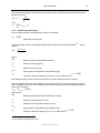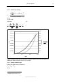
1
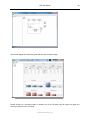
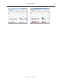
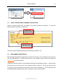
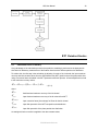
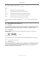
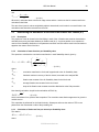
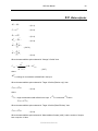
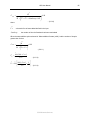
INTEGRATED GEOMETALLURGICAL SIMULATOR
USER MANUAL
SGS Canada Inc.
1140 Sheppard Ave West Unit # 6, Toronto, Ontario, Canada M3K 2A2
Tel: (416) 633-9400 Fax: (416) 633-2695 www.met.sgs.com www.ca.sgs.com
Member of the SGS Group (SGS SA)
IGS User Manual
Table of Contents
Getting Started ........................................................................................................................................1 1. Introduction.....................................................................................................................................1 2. System Requirements ....................................................................................................................1 3. Installation ......................................................................................................................................1 4. Uninstallation ..................................................................................................................................1 Operating Guide......................................................................................................................................2 5. Main Window Overview ..................................................................................................................2 6. Project File Management................................................................................................................5 6.1. Creating New Project.............................................................................................................6 6.2. Opening Existing Project .......................................................................................................6 6.3. Save Project ..........................................................................................................................7 6.4. Save Project as New project..................................................................................................7 6.5. Close Project .........................................................................................................................8 7. Flowsheet Management .................................................................................................................9 7.1. Creating a New Flowsheet.....................................................................................................9 7.2. Open Flowsheet.....................................................................................................................9 7.3. Save Flowsheet ...................................................................................................................10 7.4. Import Flowsheet .................................................................................................................12 7.5. Export Flowsheet .................................................................................................................12 7.6. Export Flowsheet to Image ..................................................................................................13 7.7. Modify Flowsheets ...............................................................................................................14 8. Data Management ........................................................................................................................16
8.1. Select Dataset .....................................................................................................................16 8.2. Import Data Sets..................................................................................................................17 8.3. View Data Sets ....................................................................................................................18 9. Grinding Simulation......................................................................................................................18 9.1. Select Dataset .....................................................................................................................18 9.2. Configure Grind Circuit ........................................................................................................19 9.3. Simulation and Reporting ....................................................................................................19 10. Flotation Simulation ......................................................................................................................21 10.1. Select Dataset .....................................................................................................................21 10.2. Configure Flotation Circuit ...................................................................................................21 10.2.1. Creating Flowsheet ..................................................................................................21 10.2.2. Units Configuration...................................................................................................23 10.2.3. Stage Setup..............................................................................................................24 10.3. Simulation and Reporting ....................................................................................................26 Appendix A – Flotation Model
SGS Minerals Services
i
IGS User Manual
1
Getting Started
1. INTRODUCTION
Integrated Geometallurgical Simulator (IGS) is a comminution and flotation simulation tool for production
forecasting and circuit design. The simulation parameters are extracted from standard tests, Minnovex
Flotation Test (MFT) for flotation and SAG Power Index (SPI) for comminution.
2. SYSTEM REQUIREMENTS
Operating System: Windows XP Service pack 3
Windows Vista Service Pack 1
Windows 7
Software: Microsoft .NET Framework 4.0
Microsoft SQL Server 3.5 SP2 Compact Edition
3. INSTALLATION
Execute the installer file provided in the SGS USB key and follow the instructions. All required software,
Microsoft .NET Framework 4.0 and Microsoft SQL Server Compact Database, will be downloaded by the
installer.
Note: Administrative privileges are required to install Microsoft .NET Framework 4.0 and
Microsoft SQL Server Compact Edition.
If you have not received a SGS USB key, the install file
can be downloaded from http://www.met.sgs.com.
Place mouse over Applications and select Integrated
Geometallurgical Simulator. Click on the download link
and fill out the registration form.
4. UNINSTALLATION
To uninstall IGS, open [Control Panel] via the start
menu under settings. Double click on [Add or Remove
Programs]. Scroll down and select IGS. Click uninstall and follow the instructions.
SGS Minerals Services
2
IGS User Manual
Operating Guide
5. MAIN WINDOW OVERVIEW
Double click on the IGS icon will start the program and the following main window is displayed on the
screen.
Menu bar
options
Status bar:
Displays Dataset name,
flowsheet name, and simulation
status
The flotation main window (default) will appear after creating a new IGS project.
Simluation type
tab
Flotation circuit
construction
frame
Stage reporting
frame
Flotation unit
property frame
Selected dataset
name
Selected flowsheet
name
SGS Minerals Services
IGS User Manual
Clicking on the Grinding tab will change to the grinding main window interface.
The tabs will be automatically selected based on the active dataset. The flotation tab is selected when
the active dataset contains both grinding and flotation block data. As default, the flotation tab will be
automatically selected when no active dataset is selected.
SGS Minerals Services
3
IGS User Manual
Menu Bar Options:
• File:
New: Create new project
Open: Open existing project
Save: Save project
Save As: Save project as a new project file
Close: Close the project
Exit: Exit IGS program.
•
Edit:
Undo: Undo last action
Redo: Redo previous action
Delete: Delete selection
Cut: Cut selection to clipboard
Copy: Copy selection to clipboard
Paste: Paste clipboard to cursor
•
View:
Zoom in: Zoom In by 25%
Zoom out: Zoom Out by 25%
Reset: Reset zoom to 100%
•
Flowsheet:
New Flowsheet: Create a new flowsheet
Open Flowsheet: Open an existing flowsheet
Save Flowsheet: Save the flowsheet
Import Flowsheet: Import a flowsheet from file
Export Flowsheet: Export the flowsheet to file
Generate Flowsheet to Image: Export flowsheet to picture (PNG format)
Modify Flowsheets: Rename and delete saved flowsheets
•
Data:
Import Data: Import dataset from file
Modify Data: Edit dataset name and description and delete datasets
Select Data: Select dataset for simulation
•
Grinding:
Configure: Configure grinding circuit inputs
Simulate: Simulate grinding circuit
•
Flotation:
Simulate: Simulate the flotation circuit
Order Connections: Set stream reporting order
•
Help:
About: Software information
Status Bar
• Dataset:
Display selected dataset name
•
Simulation status
Message display when simulation is complete or failed
SGS Minerals Services
4
IGS User Manual
5
6. PROJECT FILE MANAGEMENT
The IGS project file is a database containing multiple flowsheets and datasets. The database structure is
show below.
The flowsheets are constructed and configured by the user while the datasets are provided by SGS and
are vital for simulation. There are two sub categories of datasets, flotation and comminution feed. The
flotation feed contains mineral floatability data and the comminution feed contains ore’s grindability data.
Appropriate datasets need to be loaded for the specific type of simulation.
SGS Minerals Services
IGS User Manual
6.1.
CREATING NEW PROJECT
1) To create a new project file, select [File] on the menu bar and click [New].
2) Enter a project name and select the destination folder. Then click [Save].
Destination folder
Enter project
name
6.2.
OPENING EXISTING PROJECT
1) To open an existing project file, select [File] on the menu bar and click [Open].
2) Navigate to the folder where the project file is located.
3) Select the project file and click [Open] or double clicking the project file.
SGS Minerals Services
6
IGS User Manual
7
Destination folder
Select project to
open
6.3.
SAVE PROJECT
1) To save the active project, select [File] on the menu bar and
click [Save].
6.4.
SAVE PROJECT AS NEW PROJECT
1) To save the active project as a new IGS project file, select [File] on the menu bar and click [Save As].
2) Navigate to the destination folder. Enter an IGS project name and click [Save].
SGS Minerals Services
IGS User Manual
8
Destination folder
Enter new IGS
project name
6.5.
CLOSE PROJECT
1) To close the active project, select [File] on the menu bar and click [Close].
2)
A save changes prompt will appear. Click [Yes] to save changes, [No] to discard changes, or
[Cancel] to cancel the close action. Any changes made on the active flowsheet will be lost.
SGS Minerals Services
9
IGS User Manual
7. FLOWSHEET MANAGEMENT
A flowsheet is defined by a comminution circuit and a flotation
circuit. The circuit to be simulated is dictated by the feed data.
Multiple flowsheets can be saved in one project file and can be
loaded as needed.
7.1.
CREATING A NEW FLOWSHEET
1) Click on [Flowsheet] on the menu and select [New flowsheet]
2) A prompt window will appear asking to save the current
flowsheet.
3) Click [Yes] to save the current active flowsheet. Click [No] to discard the current flowsheet.
Note: The new flowsheet will not be saved when created. A save action is required to save
the flowsheet to the project file.
7.2.
OPEN FLOWSHEET
Open a flowsheet saved in the project file.
1) Click on [Flowsheet] on the menu and select [Open Flowsheet]
2) Select the desired flowsheet to open and click [Open].
saved flowsheet and all its inputs will be loaded.
SGS Minerals Services
The
10
IGS User Manual
Flowsheet name
and author
Selected
flowsheet
Flowsheet created
and last modified
time stamp
Flowsheet
description
3) A prompt window will appear asking to save the current flowsheet before openning. Click [Yes] to
save, [No] to discard or [Cancel] to cancel the open flowsheet action.
7.3.
SAVE FLOWSHEET
Save the flowsheet into the project file.
1) Click on [Flowsheet] on the menu and select
[Save Flowsheet].
2) Enter a flowsheet name and description.
click [Ok].
Then
Both the comminution and flotation
circuit flowsheet will be saved as well as the units’
inputs.
SGS Minerals Services
11
IGS User Manual
Note: A name must be given to save the flowsheet. If the field is empty, a red outline will
appear around the name box.
Error indicator
SGS Minerals Services
12
IGS User Manual
7.4.
IMPORT FLOWSHEET
A flowsheet can be imported from a file (*.igsflsh).
This will
import the saved flowsheet and its inputs.
Note: Flowsheet files do not contain datasets.
1) To import a flowsheet, select [Import] under [Flowsheet] on
the menu bar.
2) Navigate to the destination folder and select the flowsheet file
(*.igsflsh). Click [Open]
Destination
folder
Select flowsheet
file
Note: Imported flowsheet will not be automatically saved into the project file. Refer to 7.3 to
save the flowsheet into the project file.
7.5.
EXPORT FLOWSHEET
The active flowsheet can be exported to a file (*.igsflsh).
parameters will be saved in the flowsheet file.
Note: The datasets will not be exported.
SGS Minerals Services
The flowsheet diagram and the inputs
IGS User Manual
13
1) To export flowsheet, select [Export] under [Flowsheet] on the
menu bar.
2) Navigate to the destination folder and enter a name for the
flowsheet. Press [Save].
Destination
folder
Enter flowsheet
filename
7.6.
EXPORT FLOWSHEET TO IMAGE
The active flowsheet can be exported for reporting. This option will save the active flowsheet as a
portable network graphics file (*.png).
1) Click on [Flowsheet] on the menu and select [Generate
Image].
2) Navigate to the destination folder and enter a filename. Click
[Save].
SGS Minerals Services
IGS User Manual
14
Destination
folder
Enter flowsheet
filename
7.7.
MODIFY FLOWSHEETS
Each flowsheet is assigned a name and description upon saving. The flowsheet name and description
can be modified through the [Manage Flowsheets] window. Flowsheets can also be deleted from the
same window.
1) To open the flowsheet management window, click on [Flowsheet] on the menu and select [Modify].
2) To delete a flowsheet, click the [Delete] button associated to the flowsheet. Click [Yes] on the
confirmation pop-up to delete.
SGS Minerals Services
IGS User Manual
15
Edit flowsheet
name and
description
Delete flowsheet
permanently
1) To modify the flowsheet name and description, click on [Edit] associated to the flowsheet. The
flowsheet name and description will become editable.
Flowsheet name
edit box
Flowsheet description
edit box
2) Click [Save] to save the changes. Press [Cancel] to discard the changes.
3) Press [Close] to exit the flowsheet management.
SGS Minerals Services
IGS User Manual
16
8. DATA MANAGEMENT
The dataset files (*.igsdata) are vital for simulation and are provided by SGS. It contains all the mineral
floatability and ore grindability information.
8.1.
SELECT DATASET
A dataset containing the appropriate feed must be selected to run a
simulation.
1) To select the appropriate feed information or use another change the
dataset for simulation, select [Data] and select [Select].
2) Click on the dataset to be used for the simulation and click [Select]. To cancel the selection, click
[Cancel]. The selected dataset’s name will appear in the status bar.
SGS Minerals Services
17
IGS User Manual
Selected
dataset
Flotation feed
minerals
Feed created and
last modified times
stamp
General feed
information
8.2.
IMPORT DATA SETS
1) To import a dataset (*.igsdata), click on [Data] and select [Import].
2) Navigate to the folder where the datasets are located, select the desired dataset file and click [Open].
Note: Importing additional dataset files will append to the list of datasets in the project file.
SGS Minerals Services
IGS User Manual
18
Destination
folder
Select
dataset file
8.3.
VIEW DATA SETS
To view the block data of a dataset, select a data set and click [View]. A maximum of 100 blocks will be
displayed. Click [Close] when finished.
9. GRINDING SIMULATION
9.1.
SELECT DATASET
Datasets containing grinding feed must be loaded for simulation.
To select the dataset, follow the
instructions outlined in 8.1. If a dataset containing both flotation and grinding feed is selected, only the
grinding feed will be used in the simulation.
SGS Minerals Services
19
IGS User Manual
9.2.
CONFIGURE GRIND CIRCUIT
1) To configure the grinding circuit, click on [Grinding] tab on the left side of the main window. A
graphical representation of a typical autogenous-ball mill circuit will appear.
Invalid input
2) Fill out the input paramter form with appropriate values and click [Ok].
Note: Invalid inputs are indicated by a red outline around the input field. Place mouse over
the input field will display an error tooltip. All input fields must be clear of errors in
order to continue.
Tips: Placing the mouse over the input field will display a tooltip with detail description of the
input parameter.
9.3.
SIMULATION AND REPORTING
SGS Minerals Services
IGS User Manual
20
With the appropriate dataset selected and the
flowsheet configured, click on [Grinding] on the
menu bar and select [Simulate].
Once the
simulation is complete, a report window will appear.
The first tab displays the result summary.
The second to fifth tab display the cumulative
distribution plots for feed, bond work index (BWi),
SAG power index (SPI), circuit throughput, specific
power, and transfer and product size. The limiting
throughput plot is also included in the reporting
window.
The simulation results can be exported to excel (*xls, *.xlsx) or csv file. Click on [Export] on the report
menu bar and select [Results]. Browse to the folder where the file will be saved, enter a filename, and
SGS Minerals Services
21
IGS User Manual
click [Save]. The simulation summary, detailed block output, the circuit configuration parameters, and the
report plot’s x-y coordinates are reported.
To save the simulation report, click on [Export] on the report menu bar and select [Save report]. Browse
to the folder where the file will be saved, enter a filename, and click [Save]. To open an existing report,
click on [File] on the main window menu bar and select [Open report]. Browse to the folder where the
report file is located, open the file by selecting the file and click [Open] or by double-click on the file.
10. FLOTATION SIMULATIONS
10.1.
SELECT DATASET
Datasets containing flotation feed must be loaded for simulation.
To select the dataset, follow the
instructions outlined in 8.1. If a dataset containing both flotation and grinding feed is selected, only the
matching blocks in both flotation and grinding feed will used in the simulation. The matching blocks in the
grinding feed will be used to simulate the expected product size and throughput for each block. The
results are then used as feed parameters for flotation simulation. Unmatching blocks are ignored and will
not be simulated.
10.2.
CONFIGURE FLOTATION CIRCUIT
10.2.1.
Creating Flowsheet
1) Right click anywhere on the flowsheet construction frame to
bring out a list of flotation unit icons.
2) Click on the desired unit will place the unit icon on the
construction frame.
Note: All flotation circuits must begin with a [Feed] unit
and end with [Product] units.
3) Placing a [Feed] and [Mechanical Bank] units on the
construction frame looks like the following (below). The
added units are also listed in the stage reporting frame.
SGS Minerals Services
22
IGS User Manual
Error indicator
List of units
Input/output ports
Note: Notice the red dot on the top left corner of the unit. This indicates that the unit is not
properly configured. Right click on the unit and select [Show Errors] to display the
error list associated with the unit.
Note: The yellow dots indicate the unit’s input and output ports.
Here, showing the
mechanical bank’s input and output ports. These ports are used to connect the units
together.
4) To move the units around the frame, place mouse over the center of the unit icon and the mouse
cursor will change into
. Click and drag the unit to the desired location in the construction frame.
5) To connect the units, mouse over the output ports (indicated by yellow dots). The mouse cursor will
turn into
. Click and drag to another unit’s input port (also indicated by yellow dots). If the unit
SGS Minerals Services
IGS User Manual
cannot be connected at the cursor’s location, the cursor shape will turn into
23
. The mouse cursor
will indicate that the input port can be connected with.
6) Repeat steps 2 to 7 until the flowsheet is constructed.
7) Save the flowsheet by clicking on [Flowsheet] on the menu bar and select [Save]. Enter a name and
a description and click [Ok].
10.2.2.
Units Configuration
Each unit needs to be manually configured. All newly created units will have typical values set. Select a
unit on the construction frame stage or the stage view frame and the unit’s configuration inputs will
appear in the unit property frame.
SGS Minerals Services
IGS User Manual
Tip:
24
Placing the mouse over an input parameter will display the detailed description of the
input parameter.
Note:
An invalid input will cause a red outline around the text box. A red dot will also be
placed on the top right corner of the corresponding unit on the construction frame.
10.2.3.
Stage Setup
Several units can be grouped into one stage. The stage will be reported as a single unit with one feed
and two output streams (concentrate and tails). This feature is useful for looking at the grade and
recovery across several units as one cohesive unit.
1) To setup a stage, right click on the stage view frame and select [Add Stage].
2) Click and drag the units to be reported in that stage.
SGS Minerals Services
IGS User Manual
25
3) To delete a stage, right click on the stage name and select delete. All units grouped under the
deleted stage will be automatically moved out of the stage.
4) To name a stage, select the stage and enter a name for the stage in the [Name] field in the unit
property frame. Repeat for all stages.
Stage name
SGS Minerals Services
26
IGS User Manual
5) The stage input(s) and output(s) need to be specified. Below the [Name] field, specify the streams
that make up the stage’s feed, concentrate, and tails stream. Repeat for all stages.
Feed stream
components
Concentrate stream
components
Tails stream
components
6) Repeat steps 1 to 5 to create additional stages.
10.3.
ORDER CONNECTIONS
The stream reporting order can be changed. By default, IGS reports the stream in the order they are
created. To change the stream order, click on [Flotation] on the menu bar and select [Order Connections].
SGS Minerals Services
27
IGS User Manual
Each stream can be identified by the source unit’s output node
or by the destination unit’s input node. By default, the stream
is identified by the source unit’s output node.
The stream
name can be changed to the destination unit’s input node by
click on [Toggle].
To move a stream, select the stream and click on one of the
four movement buttons.
Clicking on [Ascending] or [Descending] will automatically
order the stream names alphabetically.
Click [Ok] when finished or [Cancel] to discard the changes.
10.4.
SIMULATION AND REPORTING
With the appropriate dataset selected and the flowsheet constructed, click on [Flotation] on the menu bar
and select [Simulate]. Once the simulation is complete, a report window with two tabs will appear.
The first [Flotation] tab displays the flowsheet constructed by the user.
The unit parameters are
unchangeable in this window.
At the bottom of the [Flotation] tab, each stream’s solid and volumetric flows are reported as well as the
maximum solid and volumetric flow and maximum percent solids.
SGS Minerals Services
IGS User Manual
28
The second [Stage] tab reports the grade and recovery across the stage.
Double clicking on a mechanical bank or flotation unit in the [Flotation tab] will report the grade and
recovery across the unit in a new tab.
SGS Minerals Services
IGS User Manual
SGS Minerals Services
29
IGS User Manual
30
Double clicking on other units (feed, product, junction, etc) or streams (lines connecting two units) will
report the metal and mineral grade, flotation kinetics (kavg and Rmax), stream percent solids, and
throughput (mass, water, and volume flow). For feed, junctions, and modifier units, the output stream is
reported.
To view the metals and minerals results of specific blocks, click on [Tools] and select [Select block(s)]. A
pop-up window will appear with a list of blocks that were in the dataset. Click on the block(s) of interest
and click [Select]. To select multiple blocks, hold down control (Ctrl) when clicking on the blocks. A
maximum of 10 blocks can be selected at once.
The simulation results can be exported to excel (2003, 2007, and 2010) or csv file. Click on [Export] on
the report window’s menu bar and select [Results]. Browse to the folder where the file is to be saved,
enter a filename, and click [Save]. The report file reports the mass/water recoveries, mineral and metal
grade, and flotation kinetics of each mineral for each block in the dataset. The mechanical bank and
flotation column performance are also reported.
11. FLOTATION BENCHMARK
IGS can automatically benchmark plant survey data with MFT simulation results. This functionality is
enabled by the dataset provided by SGS Canada. When a dataset with benchmark functionality enabled,
the [Benchmark] option will appear under [Flotation] on the menu bar.
SGS Minerals Services
IGS User Manual
11.1.
31
SELECT DATASET AND FLOWSHEET CONSTRUCTION
Datasets containing flotation feed and flotation survey must be loaded for simulation. To select the
dataset, follow the instructions outlined in 8.1.
Flotation Feed
Data (Block Data)
Flotation Survey
Data (Plant Data)
Construct the plant’s flowsheet by following the instructions outlined in 10.2.
11.2.
BENCHMARK AND REPORTING
With the appropriate dataset selected and the flowsheet constructed, click on [Flotation] on the menu bar
and select [Benchmark]. If the [Benchmark] option is not available, please contact SGS Canada at
[email protected] for more information.
A dialog with objective function error will appear indicating the benchmarking progress. A report window
will pop-up when the minimum error of the objective function is reached. The first two tabs plots the
survey data versus simulated data on two different axes (linear and logarithmic). The remaining two tabs
are standard flotation simulation report tabs. See section 10.4 for more information.
SGS Minerals Services
IGS User Manual
32
12. OPTIMIZATION
IGS can automatically optimize the froth recovery to achieve the user’s desired grade and recovery ratio.
This functionality is enabled by the dataset provided by SGS Canada. When a dataset with optimization
functionality enabled, the [Optimize] option will appear under [Flotation] on the menu bar.
12.1.
SELECT DATASET AND FLOWSHEET CONSTRUCTION
Datasets containing flotation feed and an optimization target must be loaded for simulation. To select the
dataset, follow the instructions outlined in 8.1.
Construct the plant’s flowsheet by following the instructions outlined in 10.2.
12.2.
OPTIMIZATION AND REPORTING
With the appropriate dataset selected and the flowsheet constructed, click on [Flotation] on the menu bar
and select [Optimize].
If the [Optimize] option is not available, please contact SGS Canada at
[email protected] for more information.
A dialog indicating the optimization progress will appear. Once complete the standard flotation report
window will pop-up. See section 10.4 for more information.
SGS Minerals Services
IGS User Manual
SGS Minerals Services
33
IGS User Manual
APPENDIX A
FLOTATION MODEL
SGS Minerals Services
34
35
IGS User Manual
1.0
1.1
IGS: Flotation Model
Flotation Simulation
IGS is mathematical simulation software used to simulate a metallurgical operation to forecast the
metallurgical production. It is also a powerful tool to monitor the operation.
IGS employs a new mathematical model. FLEET used an iterative process where each unit is calculated
until convergence before moving to the next unit. This method uses multiple nested loops which are very
repetitive and time consuming. For flowsheets involving recycles, convergence will most likely not
reached after the set maximum amount of iteration allowed. This obstacle was overcome with IGS by
using a matrix of simultaneous equations to balance the entire circuit. Like the FLEET software, the
flotation inputs for IGS are gathered from MFT tests.
1.2
System of Simultaneous Linear Equations
IGS employs the system of linear equations (Ax = b) to solve the flowsheet, where A is a matrix
representing the flowsheet configuration, x is the result vector (column matrix), and b the constraint
vector. The constraint vector contains the solid and water going into the system. The matrix is solved for
each mineral rate.
The flowsheet, constructed by the user, can be represented using a matrix. The flowsheet configuration
matrix is built as the user creates and joins the units together. For each newly created unit, the builder
appends new row corresponding to the number of output port(s) and new column corresponding to the
number of input port(s). For example, fresh feed unit has one output, mechanical bank cells and flotation
column units have three ports (one input, two outputs), and junctions have multiple inputs and one output.
The rows and columns that represent a specific unit are arranged in the order of input then output(s). For
units with more than one output, the concentrate precedes the tails.
Once the flowsheet matrix is setup, a number of systematic steps are taken to reduce the matrix by
substitution and decomposed into an upper and lower triangular matrix.
1.3
Calculation Sequence
The calculation sequence used by IGS is vastly different from FLEET because of the new mathematical
model. The calculation sequence is depicted below.
SGS Minerals Services
36
IGS User Manual
2.0
2.1
Flotation Kinetics
Correction of Rmax and kavg
A key advantage of the calculation process is that predictive modeling is performed at the plant particle
size based on laboratory measurement of the flotation kinetics with a different particle size distribution.
To achieve this, the first step in the calculation is adjusting, for each of the I minerals, the input maximum
recovery and rate constant values from the SGS flotation test (MFT) particle size to the plant particle size
using a correction factor calculated in the MFT parameter extraction process. A linear adjustment is made
to the maximum recovery values:
(
)
F
I
I
I
I
Rmax,
I = RmaxSlope, I × P80,MFT − P80, Plant + Rmax,I
…(2.2.1)
where
F
Rmax,
I
I
max,I
R
I
maxSlope, I
R
P80I ,MFT
I
80, Plant
P
feed fractional maximum recovery of the Ith mineral
input fractional maximum recovery of the Ith mineral from MFT
input correction factor (linear slope) for Rmax for the Ith mineral
input 80th percentile of the MFT test particle size distribution
input 80th percentile of the plant particle size distribution
An analogous linear correction is applied to the rate constant values:
SGS Minerals Services
37
IGS User Manual
(
)
F
I
I
I
I
k avg
, I = k avgSlope, I × P80, MFT − P80, Plant + k avg , I
…(2.1.2)
where
F
k avg
,I
feed flotation rate constant of the Ith mineral
k
I
avg , I
k
I
avgSlope, I
input flotation rate constant of the Ith mineral from MFT
input correction factor (linear slope) for kavg for the Ith mineral
I
80, MFT
P
input 80th percentile of the MFT test particle size distribution
I
80, Plant
P
input 80th percentile of the plant particle size distribution
For the remainder of the calculations, all references to
values.
2.2
Determining the rate constants - kI,J
2.2.1
Description
Rmax,I
and
k avg , I
refer to these corrected feed
For the modeling it is necessary to use fixed k values as the k distribution cannot be passed directly into
the recovery calculation. Therefore, for each of the I = 1..N minerals, J = 1..M individual k values must be
calculated for each distribution. This section describes the method of calculating the kI,J values.
2.2.2
Calculating kmax
The kmax value is determined from the kavg and α (alpha) values for each of the I minerals by the
following equation:
k max,I =
k avg ,I
αI
(
)
⎛ F eα I − 2 + 1 ⎞
⎟⎟
× ln⎜⎜
1− D
⎝
⎠
…(2.2.2.1)
where Orivaldo takes F = D = 0.9999
kmax is the 99.99th percentile of the k distribution: this is an adequate approximation for our purposes.
If
kavg , F , I
2.2.3
is less or equal to 0.001, kmax=0
Calculating kmultiplier
Once kmax is determined for the Ith mineral, this value is multiplied by a fixed, arbitrarily defined set of k
ratios, defined here as kmultiplier, to define the edges (denoted kj where j = 1.. M) of the bins (denoted kJ
where J = 1..M) that will be used to approximate the k distribution for each of the I minerals. The
kmultiplier progression for all minerals is given by:
SGS Minerals Services
IGS User Manual
38
k multiplier for mineral I = 1..N
3.5
3
2.5
2
1.5
1
0.5
0
1 2 3 4 5 6 7 8 9 10 11 12 13 14 15 16 17 18 19 20
Bin [J]
The values that exceed one are not used any further in the calculation and hence the progression is
effectively given by:
k multiplier for mineral I = 1..N
1.2
1
0.8
0.6
0.4
0.2
0
1
2
3
4
5
6
7
8
9
10 11 12 13 14 15
Bin [J]
It is evident that this set of ratios is nearly linear, resulting in a slight bias towards a greater number of
bins at low k values. The theoretical basis for a greater number of bins at low k is well founded and this
distribution should be examined in terms of the number of bins required and the relative distribution of
those bins (relative to kmax) to optimize the accuracy vs calculation speed.
sValue =
2.2.4
1
1+ e
−( normalisedBinEdgePosition−0.5 )sigmoidSteepness
Calculating kI,J
The first bin centre is taken to be zero. The remaining bin centres are simply determined as the average
of two consecutive k values in the distribution yielding:
k I , J =1 = 0
SGS Minerals Services
IGS User Manual
and
k I , J = 2..M =
39
k I , j −1 + k I , j
2
…(2.2.4.1)
Where the j values are taken to be the bin edge values and the J values are the bin centres used in the
calculations that follow.
The ratio of the kj and kJ values multiplied by alpha is determined, but this ratio is not used further in the
calculations and should be removed from the code.
2.3
Determining the distribution of the feed in the flotation rate classes (kI,J)
2.3.1
Description
The proportion of the Ith mineral in the feed falling in each of the J flotation rates must be determined to
calculate the recovery and mass balance per flotation rate (kI,J). A cyclone partition curve equation is
used to fit the floatability distribution in the parameter extraction and is therefore used in the simulation to
apportion the mass to each of the bins.
2.3.2
Calculation of mass fractions per floatability class
The equation to calculate the cumulative mass fraction in each floatability class is given by
*
Fcum, I , J = 1 − Rmax,
I
kI , J
⎛
⎞
⋅α
⎜ e kavg , I I − 1 ⎟
*
⎜ k
⎟
+ Rmax,
I
⎜ k I , J ⋅α I
⎟
⎜ e avg , I + eα I − 2 ⎟
⎝
⎠
…(2.3.2.1)
where
Fcum,I , J
cumulative mass fraction of mineral I apportioned to the Jth floatability class
*
max,I
R
fractional maximum recovery of the Ith mineral, corrected to the analysis P80
kI ,J
flotation rate constant of the Jth floatability class for the Ith mineral
kavg,I
average flotation rate constant for the Ith mineral
αI
slope of the flotation rate constant cumulative distribution at the 50th percentile
Note that this calculation is split into the calculation of EAUX by
kI , J
EAUX = e
kavg , I
⋅α I
…(2.3.2.2)
which is substituted in to yield the above equation. The cumulative mass fraction appears to be given the
variable name r.
This calculation is performed for the fresh feed only. Subsequent cells use the values of TPH or are
passed from the concentrate or tails of the preceding cell.
2.3.3
Calculation of feed mass flow per mineral per floatability class
The relation
M& cum, I , J = M& × FI × Fcum,I , J
…(2.3.3.1)
where
SGS Minerals Services
IGS User Manual
M& cum, I , J
cumulative mass flow of the Ith mineral in the Jth floatability class
M&
mass flow of the total feed to the unit
FI
mass fraction of the Ith mineral relative to the feed, also referred to as the assay value
Fcum,I , J
cumulative mass fraction of mineral I apportioned to the Jth floatability class
follows from the definition.
Also,
M& I ,0 = M& cum, I ,0
…(2.3.3.2)
and
M& I , J = M& cum,I , J − M& cum,I , J −1
…(2.3.3.3)
follow from the definition of the cumulative distribution.
SGS Minerals Services
40
41
IGS User Manual
3.0
3.1
Mechanical Bank
Recovery
For each mechanical bank, the recovery of each mineral is calculated by balancing the amount of water
and solids entering and exiting the system. The two compartment model by Savassi is used to calculate
the solid flow and one of the three mechanisms is used to calculate the water recovery.
The recovery of each mineral and water across each ‘stage’ or cell must be calculated for the mass
balance. The two compartment model of Savassi is used to calculate the solids mass flow and one of
three mechanisms are used to calculate the water recovery.
3.1.1
Residence Time
IGS first calculates the residence time required using the following formula:
τ=
V
Qw
…(3.1.2.3)
where
τ
residence time of the cell
V
Q&
volume of the ‘stage’ where
total
V = N cellVcell
volumetric flow of the feed to the cell, as opposed to the technically correct tails basis
and
M&
Q& total = ∑ I , J + Q& w
I , J SG I
…(3.1.2.4)
where
SGI ,J
specific gravity of the Ith mineral
Q& w = M& w
volumetric or mass flow rate of the water since SG = 1
3.1.2
Water Balance
Once the residence time is established, the water is balanced. IGS gives the user three options to
calculate water recovery:
Percent solid of concentrate stream
Fixed water flow per cell
Fixed water flow per stage
The first water balance option is the simplest of all three. The user specifies a desired percent solids
target in the input sheet and the water recovery is calculated simply by dividing the mass flow by the
specified percent solids and then multiplying by 1 – percent solids.
The second method, fixed water flow per cell is calculated using a linear function of the froth recovery.
The equation for this is simply:
Rw = C1 + C2 R f
…(3.1.3.1)
SGS Minerals Services
IGS User Manual
42
where
Rw
water recovery
Rf
froth recovery
C1
the ‘constant’ parameter specified in the input sheet
C2
the ‘linear’ parameter specified in the input sheet
Note that the water recovery is a function of a constant parameter and froth recovery. Thus, the water
recovery may change during the simulation runs. The water recovery is dependent of froth recovery,
which is determined by solving the mass recovery until convergence. When the mass recovery
converges, the water recovery iteration begins to solve for the water recovery. Therefore, by definition
M& conc,I , J = RI , J ⋅ M& feed,I , J
…(3.1.2.2)
and
M& conc,total = ∑ M& conc, I , J
I ,J
Then the water recovery is given by
Rw =
M& conc ,total
M&
w , feed
⎛ 1
⎞
⎜⎜
− 1⎟⎟
⎝ φ conc
⎠
…(3.1.2.3)
M& conc,total
total mass flow rate
M& w
water flow rate
φ conc
concentrate solids fraction
and on a ‘stage’ basis
(1 / N )
Rw = 1 − (1 − Rw )
…(3.1.2.4)
where
N
number of cells
The final water recovery is the most complex of the three and requires the most iteration. The water flow
is specified by stages, where multiple mechanical banks are grouped together. The water recovery is
calculated, similarly to the 2nd method, for every cell and summed.
The final equation for conversion of a cell recovery to a ‘stage’ recovery is under review and the
derivation is as follows:
By definition
Rw =
Q& w,conc M& w,conc
=
Q& w, feed M& w, feed
given that SGw = 1
…(3.1.2.5)
Per the above equation
Rw =
M& s ,conc
M&
w, feed
⎛ M& S ,conc + M& w,conc ⎞
⎜
− 1⎟⎟
⎜
&
M
s ,conc
⎝
⎠
…(3.1.2.6)
therefore
SGS Minerals Services
IGS User Manual
M& s ,conc ⎛ M& s ,conc + M& w,conc − M& s ,conc ⎞
⎜
⎟
⎟
M& w, feed ⎜⎝
M& s ,conc
⎠
⎛ M&
⎞
M&
Rw = s ,conc ⎜⎜ w,conc ⎟⎟
M& w, feed ⎝ M& s ,conc ⎠
…(3.1.2.8)
43
Rw =
…(3.1.2.7)
so
Rw =
M& w,conc
M&
w, feed
3.1.3
…(3.1.2.9)
Volumetric recovery
As shown above
M&
Q& total = ∑ I , J + Q& w
I , J SG I
…(3.1.2.5)
And by definition
M& I , J ,conc = RJ M& I , J , feed
…(3.1.2.6)
Then
RJ M& I , J , feed
Q& T ,conc = ∑
+ Rw Q& w
SG I
I ,J
…(3.1.2.7)
and we can define recovery on a volumetric basis as
RQ =
3.1.4
∑
I ,J
RJ M& I , J , feed
+ RwQ& w, feed
SGI
QT , feed
…(3.1.2.8)
Water recovery
Water recovery is calculated by one of three mechanisms. The first, a water recovery specified in the
input sheet, is the simplest of the three and this value is used directly in the recovery calculation.
The second method is to use a linear function of the froth recovery to determine the water recovery. The
equation for this form is simply
Rw = C1 + C2 R f
…(3.1.3.1)
where
Rw
water recovery
Rf
froth recovery
C1
the ‘constant’ parameter specified in the input sheet
C2
the ‘linear’ parameter specified in the input sheet
It is interesting to note that if Rw is a function of Rf and Rf is a function of an input parameter, Rw may
change depending on simulation run inputs.
SGS Minerals Services
IGS User Manual
44
The concentrate percent solids calculation is performed iteratively in the sense that the water recovery is
recalculated once per loop over all simulation units. Note that this does not mean that the water recovery
– mass recovery relationship is solved within each unit for each outer loop iteration. Instead, the mass
recovery is calculated once on the basis of the last mass recovery calculation. This is likely to contribute
to a large number of loops required for convergence and instability in the model calculation.
By definition
M& conc,I , J = RI , J ⋅ M& feed,I , J
…(3.1.2.2)
and
M& conc,total = ∑ M& conc, I , J
I ,J
Then the water recovery is given by
Rw =
M& conc ,total
M&
w , feed
⎛ 1
⎞
⎜⎜
− 1⎟⎟
⎝ φ conc
⎠
…(3.1.2.3)
M& conc,total
total mass flow rate
M& w
water flow rate
φ conc
concentrate solids fraction
and on a ‘stage’ basis
(1 / N )
Rw = 1 − (1 − Rw )
…(3.1.2.4)
where
N
number of cells
The final equation for conversion of a cell recovery to a ‘stage’ recovery is under review.
The derivation of the above is as follows:
By definition
Rw =
Q& w,conc M& w,conc
=
Q& w, feed M& w, feed
given that SGw = 1
…(3.1.2.5)
Per the above equation
Rw =
M& s ,conc ⎛ M& S ,conc + M& w,conc ⎞
⎜
− 1⎟⎟
M& w, feed ⎜⎝
M& s ,conc
⎠
…(3.1.2.6)
therefore
Rw =
M& s ,conc
M&
w, feed
M&
Rw = s ,conc
M&
w, feed
⎛ M& s ,conc + M& w,conc − M& s ,conc ⎞
⎜
⎟
⎜
⎟
&
M
s ,conc
⎝
⎠
⎛ M& w,conc ⎞
⎜
⎟
⎜ M&
⎟
⎝ s ,conc ⎠
…(3.1.2.8)
…(3.1.2.7)
so
Rw =
M& w,conc
M&
w, feed
…(3.1.2.9)
SGS Minerals Services
IGS User Manual
3.1.5
45
Overall Recovery
Each of the three water flow options uses different formula to determine the water flow in the streams,
which affects the overall recovery. Using the two compartment model by Savassi, the overall recovery is
calculated by:
FR
⋅ (1 − Rwat ) + ENT ⋅ Rwat
k CZ ⋅* τ CZ ⋅ Ratt
= * CZ * CZ FR
(1+ k ⋅ τ ⋅ Ratt )⋅ (1 − Rwat ) + ENT ⋅ Rwat
*
Rovr
…(3.1.2.1)
In the terminology of this work, this is rephrased as
RI , J =
k I , J ⋅τ ⋅ R f ⋅ (1 − Rw ) + ENT ⋅ Rw
(1 + k I , J ⋅τ ⋅ R f ) ⋅ (1 − Rw ) + ENT ⋅ Rw
…(3.1.2.2)
where
RI ,J
recovery of mineral I in the Jth floatability class
kI ,J
rate constant I, J
Rf
froth recovery defined in the cell input
Rw
water recovery, based on the last iteration
ENT
τ
entrainment factor defined in the cell input
residence time
and
τ=
V
Qw
…(3.1.2.3)
where
τ
residence time of the cell
V
Q&
total
volume of the ‘stage’ where
V = N cellVcell
volumetric flow of the feed to the cell, as opposed to the technically correct tails basis
and
M&
Q& total = ∑ I , J + Q& w
I , J SG I
…(3.1.2.4)
where
SGI ,J
specific gravity of the Ith mineral
Q& w = M& w
volumetric or mass flow rate of the water since SG = 1
Note that this is for the case of fixed water recovery or water recovery as a function of Rf. For fixed
concentrate percent solids, and therefore water recovery as a function of solids recovery, the water
recovery is calculated as per the following section.
SGS Minerals Services
IGS User Manual
3.2
Concentrate and tail mass flows
By definition for all minerals and for water
M& conc,I , J = RI , J ⋅ M& feed,I , J
…(3.2.1)
and the mass balance dictates that
M& tail,I , J = M& feed,I , J − M& conc,I , J
…(3.2.2)
SGS Minerals Services
46
47
IGS User Manual
4.0
Flotation Column
The column model differs from the mechanical cell model in that:
It uses different collection zone recovery equations
The residence time is that of the particles in the column
Column flotation recovery may be limited by the carrying capacity of the bubbles or unit dimensions
The flotation kinetics in a column efficiency are lower than in a mechanical and this is represented by a
rate constant (kavg) modifier
After the collection zone recovery is calculated, overall recovery is determined from the collection zone
and froth recovery in a manner analogous to the mechanical cell model.
4.1
Definitions: Height and volume
There are several dimension of a column cell is important and used in the column cell model to calculate
the mass balance. The most important of all is the collection zone, which is where the particles adhere to
the gas bubbles.
H column
H froth
H column
H froth
Vcolumn
V froth
H airHoldup = Hcollectionε g
Hcollection = Hcolumn − H froth − HbelowSpargers
H collection
H effective
Vcollection
Veffective
H belowSp arg ers
VbelowSp arg ers
4.2
Water balance
4.2.1
Balance of the concentrate water
The concentrate water flow is calculated from the concentrate mass flow and the target concentrate solids
fraction:
SGS Minerals Services
48
IGS User Manual
Qw,conc = M w,conc =
1 − ϕ conc
ϕ conc
The concentrate water
Qw,conc
channeling through the froth
from the pulp
M s ,conc
Qw,conc, pulp
derives from three sources: the wash water
Qw,conc,channeling
Qw,conc,ww
, water from
and (potentially) water from a negative bias, known as water
:
Qw,conc = Qw,conc, ww + Qw,conc, pulp + Qw,conc,channeling
4.2.2
Wash efficiency factor
There is inefficiency in the froth referred to as channeling whereby a fraction of the feed water is not
washed from the froth by the wash water. For the purposes of calculating recovery, this entrained material
contributes to the water recovery (Rw) and entrainment. A wash efficiency factor (Ewash) is defined and
the concentrate water flow from channeling is calculated relative to the concentrate water flow:
(1 − E wash ) =
Qw,conc ,channeling
Qw,conc
Rearranging
Qw,conc,channeling= (1− Ewash)Qw,conc
4.2.3
Wash ratio and wash water
We define a wash ratio as the ratio of the wash water addition to the concentrate water flow
Wratio =
Qww
Qw,conc
Case 1:
Wash water calculated from specified wash ratio
Qww = Qw,concWratio
Case 2:
Wash water rate specified as a constant C
Qww = C
4.2.4
Bias and water from the pulp
If there is not sufficient wash water to fully displace the pulp water (negative bias):
Q < Qw,conc − Qw,conc,channeling
If ( ww
then
)
Qw,conc, pulp = Qw,conc − Qww − Qw,conc,channeling
Else if the wash water is sufficient to fully wash the froth (positive bias)
elseif (
Qww ≥ Qw,conc − Qw,conc,channeling
)
Qw,conc, pulp = 0
4.2.5
Water recovery and overall water recovery
SGS Minerals Services
49
IGS User Manual
For the purposes of calculating entrainment in the recovery equation, we define water recovery as the
water in the concentrate that derives from the feed - therefore having the pulp composition:
Qw,conc , pulp + Qw,conc ,channeling
Rw =
Qw, feed
The overall water recovery is:
Qw,conc
Rw =
Qw, feed + Qww
However, in the overall water balance for the circuit we can treat the wash water as an additional feed
stream (a junction before the column) so that it modifies the residence time correctly so in practice:
Rw =
Qw,conc
Qw, feed
4.2.6
Reporting bias velocity
For reporting, the bias velocity is required:
J bias =
Qww − Qw,conc
Ac
4.3
Residence time
4.3.1
Effective slurry superficial velocity
The vertical velocity of slurry in the column without air is given by:
J sl , noHoldup =
Qtails
Acolumn
Where
J sl,noHoldup
Superficial slurry velocity ignoring the effect of gas holdup:
Qtails
Tails volumetric flowrate including wash water
Acolumn
Cross sectional area of the column
Then the true or effective slurry superficial velocity is given by:
J sl ,eff =
J sl ,noHoldup
(1 − ε )
g
4.3.2
Slurry residence time
Assuming the effective slurry residence time is used, the slurry residence time is given by:
τ sl =
H collection
J sl ,eff
…(5)
Where:
τ sl
4.3.3
Residence time of the slurry in the collection zone
Mean particle density
SGS Minerals Services
50
IGS User Manual
The mean particle density is derived from the mass flow matrix in fractional form and the density of the
particles / minerals
M fractional , I , J =
M I ,J
∑M
I ,J
Then
ρ p = ∑ M fractional,I , J ρ I
4.3.4
Particle Reynolds Number
Given an assumed value of the particle slip velocity, for example:
U sp = 0.002
Particle slip velocity [m/s]
Particle Reynolds number is calculated using the assumed slip velocity and recalculating
relation: 1
Re p =
U sp
via the
ρ lU sp d p ,50
μf
Where:
Re p
Particle Reynolds number [dimensionless]
ρl
Density of the fluid [kg/m3]
U sp
Particle slip velocity [m/s]
d p,50
50th percentile of the particle size distribution [µm]
μf
Viscosity of the liquid (water) [Pa.s or kg.s-1.m-1]; for water at 20C
μ f = 0.001
Note that the existing column model corrects the Re for particle fraction, but this is incorrect.
Also note that the units used in the existing column model are not SI. The units used are g, cm and s,
which invalidates the value of Re, but these are used in the calculations due to constants calibrated for
these units. Therefore:
d p,50 = d p,50,input /10000
and units are:
Re p
Particle Reynolds number [dimensionless, incorrect]
ρl
Density of the fluid [tons/m3 = SG]
U sp
Particle slip velocity [cm/s], initially 0.2 cm/s
d p,50
50th percentile of the particle size distribution [cm]
μf
1
Viscosity of the liquid (water) [g.cm-1.s-1]; for water at 20C
http://en.wikipedia.org/wiki/Reynolds_number
SGS Minerals Services
μ f = 0.01
51
IGS User Manual
4.3.5
Particle slip velocity
2
⎛ dp ⎞
2.7
g ⎜⎜ 6 ⎟⎟ (ρ p − ρ l )(1 − ϕ pulp )
10 ⎠
= ⎝
0.687
0.18μ f 1 + 0.15 Re p
(
)
m 2 kg
m
m s2
m3 =
=
kg
s
m.s
kg
s 2 = m.s = m
kg
s
s2
m.s
U sp
Where
G = 981 cm/s
…(2)
0.00018
0.009
0.00016
0.008
0.00014
0.007
0.00012
0.006
0.0001
0.005
0.00008
0.004
0.00006
0.003
0.00004
0.002
0.00002
0.001
0
Usp [m/s]
Re
Unit check:
Re
Usp
0
0
50
100
150
Dp50
Particle Reynolds number and slip velocity as a function of particle size after three iterations of
substitution. Maximum relative error is 0.3% at 140µm 2 .
4.3.6
Particle residence time
Particle superficial velocity is defined as:
J p = J sl,eff + Usp
Where
2
IGS Model Development Rev 23.xls
SGS Minerals Services
52
IGS User Manual
Jp
Particle superficial velocity
J sl,eff
Effective slurry superficial velocity, accounting for gas holdup
U sp
Particle slip velocity relative to the slurry
Then
τp =
H collection
Jp
100
* 60
4.4
Recovery
4.4.1
Vessel dispersion number
The vessel dispersion number is calculated by:
Nd =
0.63Dcolumn
SuperficialParticleVelocityH collection
…(3)
Given the vessel dispersion number and particle residence time, the Dobby-Finch equation is used to
determine the a-parameter by:
4.4.2
‘a’ parameter
a = (1 + 4k J E ff τ p N d )
0.5
Where
a
kJ
a-parameter of the Dobby-Finch equation
Flotation rate constant of the Jth rate class
τp
Particle residence time
Nd
Vessel dispersion number
E ff
Efficiency factor (k-multiplier)
Then if
4.4.3
a
> 1000
Nd
;
a = 1000 N d
…(7)
Recovery in the collection zone
The recovery in the collection zone can then be calculated from:
R J ,att ,CZ
⎛ 1 ⎞
⎡
⎜
⎟
⎜ 2N ⎟
⎢
4ae ⎝ d ⎠
= 1− ⎢
a
−a
⎢
2 2 Nd
2 2 Nd
− (1 − a ) e
⎣ (1 + a ) e
⎤
⎥
⎥
⎥
⎦
Where
RJ ,att,CZ
a
Recovery of the Jth floatability class by attachment
‘a’ parameter of the Dobby-Finch equation
SGS Minerals Services
53
IGS User Manual
Nd
4.4.4
Vessel dispersion number
Recovery
Then the recovery of the Jth floatability class in the column is given by:
RJ =
RJ ,att ,CZ ⋅ R f ⋅ (1 − Rw ) + ENT ⋅ Rw (1 − RJ ,att ,CZ )
(1 − R
J ,att ,CZ
⋅ (1 − R f )⋅ (1 − Rw )) + ENT ⋅ Rw (1 − RJ ,att ,CZ )
where
RJ
recovery of the Jth floatability class
kJ
rate constant of the Jth floatability class
Rf
froth recovery defined in the cell input
Rw
water recovery
ENT
entrainment factor
SGS Minerals Services
…(8)
54
IGS User Manual
5.0
Modifier
Modifiers represent any unit that changes the floatability distribution of the feed to the product. This is
equivalent to moving mass from one floatability/particle class or rate constant bin to another. Two distinct
types of modifiers must be considered:
Concentrate modifier
Second float modifier
The models of these two types of modifier are different since they represent significantly different physical
processes.
5.1
Concentrate modifier
The concentrate modifier typically takes rougher concentrate and represents a regrind and/or chemical
change where the product has significantly lower floatability for the gangue mineral(s) and slightly
reduced floatability for the valuable minerals.
This type of modifier is typical of a copper concentrate regrind where the particles are further liberated or
‘polished’ in the regrind to remove attached gangue from the floatable particles, and/or the chemical
conditions are changed to depress floatable gangue such as pyrite.
In terms of the model, the modifier removes (subtracts) mass from some rate constant bins and adds it to
others for each mineral, based on a per-mineral kavg and Rmax multiplier and constant value, in the form
of a linear equation.
Hence, for each mineral (I):
Rmax,product,I = CR max,mod,I + M R max,mod,I Rmax,feed,I
where
Rmax,product
Maximum recovery of the product from the modifier
Rmax,feed
Maximum recovery of the feed to the modifier
CR max,mod
Rmax constant value in the modifier
M R max,mod
Rmax multiplier value in the modifier
and:
kavg, product,I = Ckavg,mod,I + M kavg,mod,I kavg, feed,I
where
Rmax,product
Maximum recovery of the product from the modifier
Rmax,feed
Maximum recovery of the feed to the modifier
Ckavg,mod
kavg constant value in the modifier
M kavg,mod
kavg multiplier value in the modifier
SGS Minerals Services
55
IGS User Manual
NOTE: In the initial design, the product rate constant values may not exceed the source values.
Therefore:
Ckavg,mod,I + M kavg,mod,I ≤ 1
If it is desirable that this constraint be lifted, the modifier and rate constant values will need to be
redesigned to allow for higher than source rate constants.
5.1.1
Mass fraction adjustment for kavg of the product
In order to calculate the mass fraction reallocation between bins it is necessary to determine the kavg of
the modifier feed.
Determining the 50th percentile of the floatable material in the feed
By definition, the kavg is the 50th percentile (median) of the rate constant distribution, excluding the
material in the 1st rate constant bin. Defining the nomenclature for this value:
kavg = k50, J =2..N
50th percentile (median) of the mass in the J=2..N rate constant classes
Consider D, the cumulative distribution of the mass fractions in the rate constant bins, excluding the first
bin:
D(k ) = ∫ X J = 2.. N
In the (unlikely) case that there is a value D=0.5, the
value.
k50, J =2..N
value is the corresponding rate constant
Now, in the cumulative distribution there are (in general) discrete values of D that fall adjacent to the 50th
percentile of the distribution at D=0.5. We will denote these
and
+
50
D
for the value immediately below D = 0.5
for the value immediately above D = 0.5. The rate constant values that correspond to these
points are denoted
k 50, J =2.. N
D50−
k50−
and
k50+
respectively. Then, by linear interpolation:
k 50+ − k 50−
=k + +
(
0.5 − D50− )
−
D50 − D50
−
50
Calculating the gamma parameter
As defined above, for a given mineral (I):
kavg,P = Ckavg,mod + Mkavg,modkavg,F
Now we define an adjustment to the rate constant distribution, γ, that will be used to redistribute the mass
between rate constant bins. Gamma is taken to be the ratio of the kavg values for the product and the
feed.
γ=
k avg , P
k avg , F
Then
γ =
C kavg ,mod + M kavg ,mod k avg , F
k avg , F
=
C kavg ,mod
k avg , F
+ M kavg ,mod
so
γ =
C kavg ,mod
k 50, J = 2.. N , F
+ M kavg , mod
SGS Minerals Services
56
IGS User Manual
Applying the gamma adjustment to the mass fractions
The rate constants for the entire simulation are fixed, so the rate constant values for the bins cannot be
adjusted. Therefore, the mass fractions in each bin must be changed to duplicate the effect of the change
in rate constant. For all J=2..N rate constants, the target product rate constant value is derived from
gamma and the Jth rate constant value:
kJ ,t arget = γ ⋅ kJ
Consider the mass fraction redistribution for a given rate constant source value
constant bins k
−
and k
+
exist that are adjacent to
−
kt arget
. The mass fraction of the source bin is linearly
+
redistributed into k and k according to the relative distance to
neighbour approach to the redistribution.
Then for each source rate
Mk,P = γMJ ,F
k J . In general, two rate
kt arget
. This is also known as a nearest
k J and its mass in the feed M J ,F
and
M k − , P + = (1 − γ )M J , F
where:
k + − k t arg et
k+ − k−
and
M k + , P + = (1 − γ )M J , F
where
M k + ,P
k t arg et − k −
k+ −k−
Mass fraction of the rate fraction bin adjacent to and above
kt arget
The deltas for each target bin are calculated for each source rate constant bin and summed. Once this is
completed, there may be too much or too little material allocated to the zero flotation rate constant bin to
satisfy the specified Rmax. The adjustment to get the appropriate Rmax is described below.
5.1.2
Mass fraction adjustment for Rmax of the product
The material in the 1st rate constant bin is the material having a flotation rate of zero and is determined
from:
X1,P = 1− Rmax,P
The adjustment to the rate constant distribution to achieve the correct Rmax after the modifier is
performed after the redistribution of material by kavg. The mass fraction of material in each of the nonzero bins is adjusted on a mass weighted basis to adjust for the mass fraction of material in the 1st
(Rmax) bin. So for each of the
ΔX J =
X J ,F
∑X
J = 2.. N
(X
1, F
J = 2..N rate constant bins:
− X 1, P )
J ,F
where:
ΔX J
The change in the mass fraction of material in the Jth rate class between the feed and
the product
SGS Minerals Services
IGS User Manual
X J ,F
The mass fraction of material in the Jth rate constant bin in the feed
∑ X J ,F
J = 2.. N
The sum of all mass fractions in the rate constant bins from bin 2 to the end of the array
X1,F
The mass fraction in rate bin one (the non-floatable material) in the feed
X 1,P
The mass fraction in rate bin one (the non-floatable material) in the product
So
X J ,F
X J ,P =
∑X
J = 2.. N
(X
1, F
− X 1, P ) + X J , F
J ,F
X J ,F
(X − X ) + X
(1 − X )
(1 − X )
=X
(1 − X )
X J ,P =
1, F
1, P
J ,F
1, F
X J ,P
1, P
J ,F
1, F
For testing purposes:
∑ X J , F = X 1,P +
J =1.. N
∑X
∑X
J = 2.. N
J = 2.. N
J ,F
(X
1, F
− X 1, P ) +
J ,F
∑X
J = 2.. N
J ,F
where:
∑X
J =1.. N
J ,F
The sum of all mass fractions in all bins, defined to be one
And
∑X
J = 2.. N
J ,F
57
= 1 − X 1, F
So
1 = X1,P + (X1,F − X1,P ) + (1 − X1,F )
which is true.
SGS Minerals Services
58
IGS User Manual
5.2
6.0
Feed
The feed is defined from the input values as follows:
M& IF = M& I × CII
…(5.1.1)
where
M& IF
M& I
C
mass flow of the Ith mineral in the feed
input mass flow of the total feed
I
I
concentration or mass fraction of the Ith mineral in the feed, also referred to as the grade
or assay
F
I
Rmax,
I = Rmax,I
…(5.1.2)
where
F
Rmax,
I
if
fractional maximum recovery of the Ith mineral in the feed. If
Rmax,I
> 100,
Rmax,I
I
max,I
R
Rmax,I
< 0.001,
Rmax,I
=0;
= 100.
input fractional maximum recovery for the Ith mineral
α IF = α II
…(5.1.3)
where
α IF
slope of the flotation rate constant cumulative distribution at the 50th percentile in the
feed
α II
If
α IF
input slope of the flotation rate constant cumulative distribution at the 50th percentile.
is less than 0.1 then
α IF
= 0.1, if
α IF
is greater than 20 then
α
flotation rate constant: see following section) and if
RI , J =
(EAUX
I ,J
(EAUX + e
− 1)
(α I − 2 )
)× R
max, I
α IF
= 20. If 0 <
F
k avg
,I
< 0.1 (the
I
I
F
k avg
,I
is greater than 200 then
α I = 200
+ 100 − Rmax,I
…(5.1.4)
where
RI , J
th
th
recovery of the J floatability class for the I mineral. When
RI , J
equal to 30 then
=100.
SGS Minerals Services
⎛ k I , J + k I , J −1 ⎞
⎜⎜
⎟⎟
2
⎝
⎠ ×α
I
k avg , F , I
is greater or
IGS User Manual
M I × RI ,1
100
•
M I ,1 =
…(5.1.5)
where
•
M I ,1
mass flow of the 1st floatability class for the Ith mineral
•
M I ,J =
M I × (RI , J − RI , J −1 )
100
…(5.1.6)
where
•
M I ,J
mass flow of the Jth floatability class for the Ith mineral
⎛ N C
SG = ⎜⎜ ∑ I
⎝ I SGI
⎞
⎟⎟
⎠
−1
…(5.1.7)
where
SG
SG I
specific gravity of the pulp solid fraction
specific gravity of the Ith mineral
• F
•
M =M
…(5.1.8)
where
•
M
mass flow total
F
CSolid = CSolid
(5.1.9)
where
CSolid
concentration solid, also referred to as percent solid
F
Solid
C
concentration solid in the feed
•
M × (100 − C Solid )
VW =
C Solid
•
…(5.1.10)
where
•
VW
volumetric flow of water
•
•
⎡ (100 − CSolid ) 1 ⎤
+
VP = M × ⎢
⎥
C
SG ⎦
Solid
⎣
…(5.1.11)
SGS Minerals Services
59
IGS User Manual
where
•
VP
volumetric flow of pulp
SGS Minerals Services
60
61
IGS User Manual
7.0
•
Junction
• S
Z
VP = ∑ V P
S =1
…(5.2.1)
where
• S
VP
•
volumetric flow of pulp in the feed streams S=1..Z
• S
Z
VW = ∑ V W
S =1
…(5.2.2)
where
• S
VW
volumetric flow of water in the feed streams S=1..Z
• S
Z
•
M I ,J = ∑ M I ,J
S =1
…(5.2.3)
where
• S
M I ,J
•
mass flow of the Jth floatability class for the Ith mineral in the feed
streams S=1..Z
M
•
M I = ∑ M I ,J
J =1
•
N
…(5.2.5)
•
M = ∑MI
I =1
…(5.2.6)
•
M
C Solid =
•
•
M +V W
× 100
…(5.2.7)
•
CI =
MI
•
M
× 100
…(5.2.8)
SGS Minerals Services
…(5.2.4)
IGS User Manual
RI ,J
•
⎛ Z S
⎜ ∑ R I , J × M IS
= ⎜ ZS =1
•
⎜
S
S
⎜ ∑ R I , 20 × M I
⎝ S =1
⎞
⎟
⎟ × 100
⎟
⎟
⎠
…(5.2.9)
where
RIS, J
recovery of mineral I in the Jth floatability class in the feed streams S=1..Z
•
M IS
mass flow of the Ith mineral in the feed streams S=1..Z
•
MI
∑
I =1 SGI
N
SG =
•
M
……(5.2.10)
SGS Minerals Services
62
63
IGS User Manual
8.0
• F
VP
VP =
NS
•
…(5.4.1)
where
NS
the number of output streams
• F
VW
NS
•
VW =
…(5.4.2)
• F
M I ,J
NS
•
M I ,J =
…(5.4.3)
•
•
MI =
M IF
NS
…(5.4.4)
•
MF
NS
•
M =
…(5.4.5)
•
M
CSolid =
•
•
×100
M +V W
…(5.4.6)
•
CI =
MI
•
× 100
M
…(5.4.7)
⎛ F
⎜ RI , J × M IF
=⎜
•
⎜ RF × M F
I
⎝ I , 20
•
RI , J
N
SG =
⎞
⎟
⎟ × 100
⎟
⎠
…(5.4.8)
•
MI
∑ SG
I =1
I
•
M
…(5.4.9)
SGS Minerals Services
Splitter
64
IGS User Manual
9.0
SG = SG F
…(5.6.1)
C I = C IF
…(5.6.2)
RI , J = RIF, J
…(5.6.3)
• F
•
M I ,J = M I ,J
•
M
J =1
N
…(5.6.4)
•
M I = ∑ M I ,J
•
Water adjuster
…(5.6?.5)
•
M = ∑MI
I =1
…(5.6.6)
When the water addition option selected is “Change % Solids” then
• F
C Solid =
M
• F
• F
I
× 100 − ΔC Solid
M +V W
…(5.6.7)
where
I
ΔCSolid
change in concentration solid defined in the input
When the water addition option selected is “Target % Solids (Dilution only)” then
I
CSolid = CSolid
…(5.6.8)
where
I
CSolid
target concentration solid defined in the input. If
I
F
CSolid
C
Solid
is less than
then
F
CSolid = CSolid
.
When the water addition option selected is “Target % Solids (Dilute/Thicken)” then
I
CSolid = CSolid
…(5.6.9)
When the water addition option selected is “Water addition flowrate (m3/h)” and the number of loops is
less or equal to 10 then
SGS Minerals Services
IGS User Manual
• F
C Solid =
M
⎛
⎞
M + ⎜⎜V W + V W × NumLoop × 0.01⎟⎟
⎝
⎠
• F
• F
• I
× 100
…(5.6.10)
where
• I
VW
volumetric flow of water added defined in the input
NumLoop
the number of time the flowsheet has been recalculated
When the water addition option selected is “Water addition flowrate (m3/h)” and the number of loops is
greater than 10 then
• F
CSolid =
•
M
× 100
⎛•F •I ⎞
M + ⎜⎜V W + V W ⎟⎟
⎝
⎠
• F
M × (100 − C Solid
VW =
C Solid
•
…(5.6.11)
)
…(5.6.12)
•
•
⎡ (100 − CSolid ) 1 ⎤
VP = M × ⎢
+
⎥
C
SG ⎦
Solid
⎣
…(5.6.13)
SGS Minerals Services
65