Download Embedded Image Segmentation on an FPGA

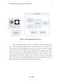
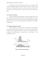
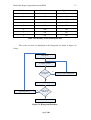
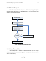
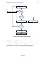
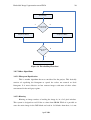
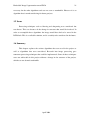
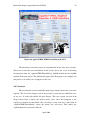
Brian Kinsella
Embedded Image Segmentation on an FPGA
B.E. Electronic & Computer Engineering
Supervisor: Dr. Fearghal Morgan
April 2008
ii
Declaration of Originality
I declare that this thesis is my original work except where stated.
Signed
…………………………
Date
…………….
iii
Acknowledgements
I, Brian Kinsella would like to thank my project supervisor Dr. Fearghal Morgan for
his constant help and advice throughout the year. His enthusiasm towards the project
was a strong driving factor for me, and encouraged me to give my best effort.
I would also like to thank the technical staff, Mr. Myles Meehan and Mr. Martin
Burke for their great help throughout the year when needed.
iv
Abstract
Field Programmable Gate Arrays are very capable devices in the area of
Digital Signal Processing. They are semiconductor devices that contain a number of
logic blocks, which can be programmed to perform anything from basic digital gate
level techniques, to complex image processing algorithms. The use of an FPGA is
advantageous over other methods in a number of ways.
Although usually slower than an Application Specific Integrated Circuit, it
gives the programmer flexibility in the design. With an FPGA the programmer can
make changes to the program as desired, whereas the user must make critical
decisions in the early design stages with an ASIC. As system requirements often
change over time, systems often need to be completely redeveloped in order to meet
demands. The cost associated with reprogramming an FPGA in the later stages of
design is negligible when compared with ASICs, which can’t be reprogrammed.
FPGAs can also be programmed very quickly, greatly reducing the time to market.
This project explores the use of FPGAs in the area of Image Processing. The
user can open a GUI and display an image, which is stored on the PC. The GUI can
then be navigated in order to modify the image by selecting from a number of image
processing functions. The processing algorithms used are selected with the idea of
recognising objects of interest in an image. The end product of this will serve to
highlight the benefits and advantages of including FPGAs in the future of Digital
Signal Processing.
v
Table of Contents
Declaration of Originality ..............................................................................................ii
Acknowledgements...................................................................................................... iii
Abstract .........................................................................................................................iv
Table of Contents...........................................................................................................v
List of Figures ..............................................................................................................vii
List of Tables ............................................................................................................. viii
Chapter 1 – Introduction ................................................................................................1
1.1 Project Background..............................................................................................1
1.2 Aim of Project......................................................................................................1
1.3 Project Specification ............................................................................................4
1.4 Chapter Layout.....................................................................................................4
1.5 Summary ..............................................................................................................5
Chapter 2 – Related Work and Methodology ................................................................6
2.1 Introduction..........................................................................................................6
2.2 AppliedVHDL......................................................................................................6
2.3 AppliedVHDLUSBSimple ..................................................................................7
2.4 Methodology ........................................................................................................7
2.4.1 Hardware.......................................................................................................7
2.4.2 Software ........................................................................................................9
2.4.3 Tools ...........................................................................................................10
2.5 Summary ............................................................................................................11
Chapter 3 – Image Processing......................................................................................12
3.1 Introduction........................................................................................................12
3.2 Processing Algorithms [4] .................................................................................12
3.2.1Grey-Scale Histogram..................................................................................12
3.2.2 Contrast Stretching......................................................................................13
3.2.3 Histogram Equalised Stretch.......................................................................13
3.2.4 Thresholding ...............................................................................................14
vi
3.2.5 Bimodal Distribution ..................................................................................15
3.3 Implementation of Processing Algorithms ........................................................15
3.3.1 Histogram....................................................................................................15
3.3.2 Differential Histogram ................................................................................16
3.3.3 Thresholding ...............................................................................................16
3.4 VHDL Implementation ......................................................................................16
3.4.1 Histogram....................................................................................................16
3.4.2 Differential Histogram ................................................................................18
3.4.3 Calculate Threshold Value..........................................................................18
3.4.4 Thresholding the Image ..............................................................................19
3.4.5 Other Algorithms ........................................................................................20
3.5 Issues..................................................................................................................21
3.6 Summary ............................................................................................................21
Chapter 4 – System Development................................................................................22
4.1 Introduction........................................................................................................22
4.2 Testing................................................................................................................22
4.2.1 Simulations .................................................................................................23
4.2.2 Final Simulation..........................................................................................24
4.3 AppliedVHDLThresholding ..............................................................................25
4.3.1 Design .........................................................................................................25
4.3.2 Analysis.......................................................................................................28
4.3.3 VB Coding ..................................................................................................29
4.3.4 Comparisons with AppliedVHDL ..............................................................30
4.4 appliedVHDLUSBThresholding........................................................................30
4.4.1 Design .........................................................................................................30
4.4.2 Analysis.......................................................................................................32
4.4.3 VB Coding ..................................................................................................33
4.5 Overview............................................................................................................33
Chapter 5 – Conclusions ..............................................................................................33
5.1 Summary ............................................................................................................33
5.2 Future Work .......................................................................................................34
References....................................................................................................................36
Appendix......................................................................................................................37
vii
List of Figures
Figure 1.1 ImageThresholder Overview ........................................................................3
Figure 2.1 Spartan 3 Starter Board [1]...........................................................................8
Figure 2.2 Digilent USB 2.0 Peripheral Communications Module[2] ..........................9
Figure 3.1 Example of an image with its histogram [3] ..............................................12
Figure 3.2 Histogram Equalisation ..............................................................................13
Figure 3.3 Image before and after equalisation ...........................................................14
Figure 3.4 Thresholding Application...........................................................................15
Figure 3.5 Histogram Flowchart ..................................................................................17
Figure 3.6 Differential Graph Flowchart .....................................................................18
Figure 3.7 Threshold Calculation Flowchart ...............................................................19
Figure 3.8 Thresholding Flowchart..............................................................................20
Figure 4.1 Histogram Simulation.................................................................................23
Figure 4.2 Differential Graph of Histogram Simulation..............................................24
Figure 4.3 Final Simulation of appliedVHDLThresholding........................................25
Figure 4.4 AppliedVHDLThreshold with GUI............................................................28
Figure 4.5 Graphed Histogram Output from appliedVHDLThresholding ..................29
Figure 4.6 appliedVHDLUSBThresholding with GUI................................................32
viii
List of Tables
Table 3.1 Boundary levels of histogram bins ..............................................................17
Table 4.1 AppliedVHDL SRAM allocation ................................................................26
Table 4.2 AppliedVHDLThresholding SRAM allocation ...........................................27
Table 4.3 Sample histogram text values ......................................................................29
Embedded Image Segmentation on an FPGA
1
Chapter 1 – Introduction
1.1 Project Background
Digital image processing is the processing and display of images. Emphasis is
placed on the modification of the image. There are three main categories of image
processing: Image enhancement, image restoration, and image classification.
Image enhancement provides more effective display of data for visual
interpretation. It helps a user to view the image and recognise different segments of an
image. An example of this is to edit the shades in an image. This technique is very
useful for assisting with distinction of different objects in an image. Rectification and
restoration of an image is another important aspect of image processing. It deals
largely with image correction, which may be necessary due to the image being
affected by geometric distortion or noise. It can also remove blurring whereby a poor
quality image may be upgraded to one with better quality and distinguishable features.
Image classification is where images are classified based on colours or shapes present
in the image. This can be useful in order for a computer to differentiate between
different types of images.
There are many useful applications of image processing. It is used as remote
sensing for robot guidance, and target recognition. It is also used for industrial
inspection, and in medial technology such as X-Ray enhancement. A very useful
application of digital image processing is to view the various colour intensities present
in an image and split the image into segments based on the results.
1.2 Aim of Project
The main objective of this project was to develop a number of image
processing algorithms for implementation on a Spartan 3 FPGA. This would follow
on from work completed in previous years to develop a Spartan-3 based embedded
system design with accompanying software and will be capable of:
April 2008
Embedded Image Segmentation on an FPGA
2
•
Generating image data
•
Sending the image data to an FPGA (Field Programmable Gate Array) board
via USB 2.0 using a PC
•
Saving the data to the onboard SRAM (Static Random Access Memory) to
allow DSP (Digital Signal Processing) functions to be performed on the image
•
Implementing the required algorithms on the image and storing the results
back in the SRAM
•
Transmitting the resulting data back to the PC to be viewed by the user
A GUI (Graphical User Interface) will be required to coordinate this activity.
The aim is to produce a system that would allow a user to perform complex digital
signal processing on an image. Faster processing speed and lower costs are, of course,
desired for this system. FPGAs allow us to perform this task at higher speed, cost
efficiency and flexibility than creating a custom ASIC for the task would allow.
A similar project was completed simultaneously using Texas Instruments
architecture. The results of both projects were to be compared on completion. Factors
such as cost, efficiency, ease of use, and of course performance would to be
compared.
In order for any person to implement this project it is strongly recommended
that they first complete the appliedVHDL semester 1 project provided by Dr. Fearghal
Morgan and familiarizes themselves with both Shane Agnew’s FYP (Real-Time
Image Warper using Digilent Spartan-3 FPGA) and Antoin O’hAllmhurain’s FYP
(DSP using Xilinx Spartan-3).
Figure
1
below
illustrates
an
overall
picture
of
the
“appliedVHDLThresholding” design and the various components required. This is the
basic data flow involved in the system. The main components are
•
A GUI for controlling the system
•
A UART for transmitting data to and from the system and the host PC
•
IOCSRBlk to control data flow to and from the UART
•
memCtrlr and datCtrlr modules
•
dspBlk, where the core functions are contained
April 2008
Embedded Image Segmentation on an FPGA
3
Figure 1.1 ImageThresholder Overview
The overall function of this system is to produce a fully segmented image
from a noisy image that is input by the user. This image will be separated into two
clearly defined regions. Depending on the image in question, there will be a number
of black and white sections. Black sections correspond to the background and white
sections correspond to the foreground. When trying to locate objects of interest this is
a particularly useful function, especially when dealing with a noisy greyscale image.
This design works on the assumption that the background and foreground will be at
different intensity levels, which will more than likely be the case.
April 2008
Embedded Image Segmentation on an FPGA
4
1.3 Project Specification
In this project a set of image processing algorithms will be performed using a
Spartan-3 FPGA. The first step will involve developing a fully functional image
histogram generator. This will consist of generating a basic image file, storing the
image in onboard SRAM and then processing the image as required. The image will
then be uploaded to the host PC, and the results verified.
After this is completed, the next step will be to load an image and implement
some extra image processing techniques on the image. These techniques will include
a differential graph of the histogram, followed by image segmentation, which splits
the image into two well-defined regions. Finally, the new image is returned the to the
host PC.
Following on from this, the system could stream an image file, via a web cam
for example, convert the image into digital and store in RAM. Also more complicated
techniques could be implemented. These techniques could include be contrast
stretching, blurring or sharpening the image, or a basic DSP filter function could be
captured from System Generator. This function could be translated to VHDL for
implementation in the system.
Results of these algorithms will be compared to the results obtained using
Texas Instruments architecture. The project should serve as a useful comparison
between the two techniques, and explore the effectiveness of an FPGA in the field of
image processing.
1.4 Chapter Layout
The subsequent chapters explore the development of the system. They also
explore previous related projects completed by other students, and talk about
problems and solutions encountered along the way.
Chapter two gives a short insight into these related projects and looks at the
methodology of the system. This includes the hardware, software and tools required
throughout.
April 2008
Embedded Image Segmentation on an FPGA
5
Chapter three is based solely on image processing. It looks into the
background of image processing, and the techniques used as well as some potential
algorithms that could be used. It also looks at some applications of image processing.
Chapter four covers the core design of the system dealing with the
development of the system, and why certain methods were chosen. It looks into how
the image processing techniques were developed and simulated on the FPGA, and
outlines any issues that arose.
Chapter five is where the conclusions of the project are outlined. This is where
accomplishments as well as future work are discussed. The report concludes with a
list of references to sources of information used throughout the year and an appendix.
1.5 Summary
A brief overview of the system and the specifications of the system are
explored here. The main components of the system are discussed. The structure of
both the project and the report were also documented in this chapter.
April 2008
Embedded Image Segmentation on an FPGA
6
Chapter 2 – Related Work and Methodology
2.1 Introduction
This chapter takes a brief look at the previous projects on which this project
was based. There are two main projects of interest involved. One named
“appliedVHDL” that was completed by the 4th year class as part of the module Digital
Design and VHDL, taught by Dr. Fearghal Morgan. The second is a project named
“appliedVHDLUSBSimple” and was completed by Shane Agnew.
There are two sides to the project being developed here. One aims to build the
system using the serial port and parallel ports on the Spartan 3 board as done in
“appliedVHDL”. The second is based on using a USB interface, as is used in
“appliedVHDLUSBSimple”.
The methodology used throughout the project is also analysed here. This
includes a description of the hardware, software and other tools that were used.
2.2 AppliedVHDL
This is the original assignment given to the 4th year class by Dr. Fearghal
Morgan for the Digital Systems Design & VHDL course. The main modules and
functions of the system are as follows.
The UART module passes control signals from the host PC to the IOCSRBlk,
and is responsible for communication with the GUI. A datCtrlr module is used to
bundle and unbundled byte wide data and 32-bit word data respectively as required.
The IOCSRBlk decodes values received from the UART, saving values into the
Control/Status registers and starting up processes as instructed. memCtrlr and
memCtrlrUnit modules are required to read from and write to RAM for both the DSP
and IO modules. A displayCtrlr module is also used to display data as it is being
transferred.
April 2008
Embedded Image Segmentation on an FPGA
7
All of the above modules are also used in this project. These modules remain
unchanged. The main focus of this project is on the dspBlk module. This is where the
functionality of the system is produced. The original appliedVHDL project consisted
of a delta subtraction of two images. One image was subtracted from the other on a
pixel-by-pixel basis.
2.3 AppliedVHDLUSBSimple
This is the project completed by Shane Agnew. This project was based on
appliedVHDL. The main difference in the two projects is that the latter uses a USB
2.0 interface. There are also a number of new DSP functions implemented in the
dspBlk module.
The system uses basically the same modules as appliedVHDL. However there
are also changes in the way the system interacts with RAM. The new DSP functions
in the dspBlk module are image rotation, colour inversion, colour change and image
morphing.
2.4 Methodology
2.4.1 Hardware
There are two main hardware components in use in this project. The FPGA
board itself, and the USB to Peripheral Communications Module
2.4.1.1 Digilent Spartan 3 FPGA Board
This is the main hardware component used in the system. This board satisfies
the need for fast processing at a low cost while providing a powerful, self-contained
development platform for designs. It features a 200K gate Spartan-3, on-board I/O
devices, and 1MB fast asynchronous SRAM. The main components of the board are:
•
200,000 gate Spartan-3 FPGA
•
2Mbit PROM (Programmable Read Only Memory)
•
1MB asynchronous SRAM
April 2008
Embedded Image Segmentation on an FPGA
•
VGA (Video Graphics Adapter)
•
RS232 serial port
•
PS/2 port
•
4 character LCD display, 8 switches, 8 LEDs 4 Buttons
•
50 MHz oscillator clock source
•
FPGA reconfiguration switch
•
JTAG port
•
Three 40-pin expansion connectors
8
Figure 2.1 Spartan 3 Starter Board [1]
2.4.1.2 Digilent USB 2 Peripheral Communications Module
The Digilent PmodUSB2 Module Board (the USB2) is used to create a USB
2.0 connection to the board. It used to exchange data with the PC. A feature of the
USB2 Peripheral Communications Module is that it can also access the JTAG
boundary scan chain. The JTAG scan chain can be used to program all on-board
devices, in this case the FPGA and the PROM. This allows the device to be
programmed much quicker, and reduces the number of cables required between the
PC and the board to just one.
April 2008
Embedded Image Segmentation on an FPGA
9
Figure 2.2 Digilent USB 2.0 Peripheral Communications Module[2]
2.4.2 Software
2.4.2.1 Digilent Adept Suite [5]
The Adept Suite provides a set of software that allows for JTAG configuration
of Xilinx logic devices and data transfer with Xilinx FPGAs via Digilent
communications modules. The Suite contains 4 pieces of software: ExPort (a JTAG
programming application), TransPort (a data transfer application), Ethernet
Administrator (an application that configures the Net1 firmware), and USB
Administrator (an application that configures the USB2 and JTAG-USB firmware).
Adept allows to configure the FPGA device, program the FPGA and to keep track of
configuration files. It can also transfer data to and from the onboard FPGA on your
system board. Read from and write to specify registers. Load a stream of data to a
register or read a stream of data from a register.
2.4.2.2 Xilinx Integrated Software Environment
Xilinx Integrated Software Environment (ISE) is a powerful, flexible
integrated design environment that allows you to design Xilinx FPGA devices from
April 2008
Embedded Image Segmentation on an FPGA
10
start to finish. ISE allows synthesis and implementation tools delivering fast place and
route times as well as high performance.
Project Navigator is the user interface that manages the entire design process
including design entry, simulation, synthesis, implementation, and finally download
the configuration of the FPGA device. Code is created and synthesised. The user can
then view an RTL schematic of the resulting circuit. PACE is responsible for placing
and routing the code for optimisation. IMPACT then generates the programming files
and downloads the code to hardware. These tools together make up Xilinx ISE, which
can be used to design and test complex digital systems.
2.4.2.3 ModelSim: Xilinx Edition
This tool partners Xilinx ISE and is used for the testing of verification of the
user’s code. The user can design a test bench to provide the stimulus to the system
that is expected when performed on the board. ModelSim then simulates the systems
behaviour due to this stimulus and graphs the behaviour of each signal on a timing
diagram. This is an extremely useful tool for error detection, as the user can see how
each signal reacts in any given circumstance relative to the other signals. This greatly
increases the speed at which a system can be designed.
2.4.3 Tools
2.4.3.1 Very High-Speed Integrated Circuit Hardware Description Language
(VHDL)
Hardware Description Languages (HDLs) enable high level program based
descriptions of hardware logic design. VHDL is one such HDL Language. This is the
language used to program the FPGA. Use of stimulus sequences and checkers (e.g.,
VHDL test benches) facilitate the simulation of VHDL models. Synthesis of VHDL
models to a target IC technology supports hardware implementation. VHDL fits well
within a structured design-documentation-test methodology for complex digital
systems.
April 2008
Embedded Image Segmentation on an FPGA
11
2.4.3.2 Universal Serial Bus 2.0
This is a serial bus standard for data transfers between interconnected devices.
USB2.0 works at a speed of 480Mb/s, bi-directional. In this project, the GUI
facilitates the transmission of data by calling C programs, which in turn call C++
functions to initiate and control USB transfers.
2.4.3.3 Microsoft Excel
Microsoft Excel is used in this project as a means to display a graph. Textual
results are written to a text file, and opened in Excel to be viewed as a bar chart.
2.5 Summary
This chapter dealt mainly with the hardware and software components and the
tools used in the system, as well as a brief overview of related projects on which this
project was based.
April 2008
Embedded Image Segmentation on an FPGA
12
Chapter 3 – Image Processing
3.1 Introduction
Fundamental image processing techniques play a very important role in this
project. There are three algorithms used in this project. Initially a histogram is
computed. Then a differential graph of this histogram is calculated. On analysis of the
differential graph, a thresholding value is chosen. The image is then segmented based
on this thresholding value. This chapter discusses the implementation of these
algorithms, as well as some other algorithms that were considered.
3.2 Processing Algorithms [4]
3.2.1Grey-Scale Histogram
The grey-scale histogram of an image represents the distribution of the pixels
in the image over the grey-level scale. It can be visualised as if each pixel is placed in
a bin corresponding to the colour intensity of that pixel. All of the pixels in each bin
are then added up and displayed on a graph. This graph is the histogram of the image.
Figure 3.1 below illustrates the histogram of a sample image. The frequencies of all
the intensity levels can be seen, and the image can be analysed based on this.
Figure 3.1 Example of an image with its histogram [3]
April 2008
Embedded Image Segmentation on an FPGA
13
The histogram is a key tool in image processing. It is one of the most useful
techniques in gathering information about an image. It is especially useful in viewing
the contrast of an image. If the grey-levels are concentrated near a certain level the
image is low contrast. Likewise if they are well spread out, it defines a high contrast
image.
3.2.2 Contrast Stretching
Contrast stretching enables the spacing of some of the output values so that
they are further apart, thereby making them more easily distinguishable. This can be
done manually by choosing the upper and lower bound of the histogram and adjusting
the graph to fit. It can also be done automatically by implementing the histogramequalised stretch.
3.2.3 Histogram Equalised Stretch
This stretch assigns more display values to the frequently occurring portions
of the histogram. In this way, the detail in these areas will be better enhanced relative
to those areas of the original histogram where values occur less frequently. The aim is
to maximise the overall contrast: as shown below, a nearly uniform (i.e. flat)
distribution is produced.
Figure 3.2 Histogram Equalisation
April 2008
Embedded Image Segmentation on an FPGA
14
As can be seen in figure 3.3 below, after an image has been equalised the
features become much more defined and easier to identify for the viewer.
Figure 3.3 Image before and after equalisation
This technique is not implemented in this project. It would be a useful addition
as it makes a clear point for thresholding much more obvious. Instead of selecting a
point out of a mostly grey image, the system can select a value between high
contrasting colours. This means that the system is more likely to select a suitable
threshold value.
3.2.4 Thresholding
A simple segmentation technique that is very useful for scenes with solid
objects resting on a contrasting background. All pixels above a determined (threshold)
grey level are assumed to belong to the object, and all pixels below that level are
assumed to be outside the object. The selection of the threshold level is very
important, as it will affect any measurements of parameters concerning the object (the
exact object boundary is very sensitive to the grey threshold level chosen).
Thresholding is often carried out on images with bimodal distributions. This is
explained below. The best threshold level is normally taken as the lowest point in the
trough between the two peaks (as above) alternatively, the mid-point between the two
peaks may be chosen.
Figure 3.4 below illustrates the application of a thresholding algorithm on a
sample image. It clearly identifies the objects of interest in the image, and removes
any noise present.
April 2008
Embedded Image Segmentation on an FPGA
15
Figure 3.4 Thresholding Application
3.2.5 Bimodal Distribution
These are images with one clear peak for the background, and one clear peak
for the foreground. The fact that an image has bimodal distribution means that it is a
suitable image for segmentation. The system will find the two peaks, and average
them. This average value is more likely to be accurate with a good bimodal image.
Figure 3.1 shows an image with its histogram. This is a good example of bimodal
distribution.
3.3 Implementation of Processing Algorithms
3.3.1 Histogram
There are two main components used in the implementation of a histogram.
These are comparators and counters. This histogram consists of 8 different intensity
levels or ‘bins’. For each bin there is one set of two comparators and a counter. If the
intensity level of the first pixel is, for example, between 0 and 32 then the counter for
the first bin will increment by 1. The pixels are read 1 at a time until the entire image
has been processed. The result of this algorithm is the value that each counter has
reached after processing.
April 2008
Embedded Image Segmentation on an FPGA
16
3.3.2 Differential Histogram
This algorithm uses the results from the original histogram algorithm to help
find the threshold point in the image. The original histogram is scanned. Each value in
the differential histogram is the subtraction of that value in the histogram from the
previous value in the histogram. This gives each peak in the histogram a negative
value in the differential curve.
3.3.3 Thresholding
The threshold value is calculated using the differential histogram. The
negative values of the curve are stored. The highest and lowest intensity values with a
peak are stored. The threshold value is calculated as the average of these points. This
is a fairly basic method of thresholding, but is effective with the majority of images. It
is particularly effective with bimodal images.
3.4 VHDL Implementation
3.4.1 Histogram
The histogram is the first algorithm to be implemented. This is done by first
comparing the pixel intensity to known values, and then incrementing the associated
histogram value. This counter is known as a histogram bin. In this project there are
eight bins used to represent the histogram of an image. Table 3.1 below illustrates the
boundaries of each bin.
April 2008
Embedded Image Segmentation on an FPGA
17
Bin Number
Lower Limit
Upper Limit
1
0
31
2
32
63
3
64
95
4
96
127
5
128
159
6
160
191
7
192
223
8
224
255
Table 3.1 Boundary levels of histogram bins
The results received on simulation of the histogram are shown in figure 3.6
below.
Histogram
Comparison State
Intensity within
boundries
N
Check next boundary level
Y
Increment Associated Counter
Take Next Pixel
N
Image Read
Finished
Y
Finished
Figure 3.5 Histogram Flowchart
April 2008
Embedded Image Segmentation on an FPGA
18
3.4.2 Differential Histogram
The differential graph of the histogram is calculated by looping through the
histogram outputs. Each value in the differential output is set to that histogram value
minus the previous histogram value.
Differential Curve
Differential level 0 =
Histogram level 0
Differential level i =
Histogram level i –
Histogram level i-1
N
Histogram
Read Done
Increment i
Y
Finished
Figure 3.6 Differential Graph Flowchart
3.4.3 Calculate Threshold Value
The threshold value is calculated by initially finding the first peak and the
final peak in the differential graph. Averaging the peaks gives the value that shall be
chosen for thresholding.
April 2008
Embedded Image Segmentation on an FPGA
19
Calculate Threshold Value
Zero
Crossing at
Differential
Value(i)
N
Increment i
Y
Peak 1 = 0?
N
Y
Peak 1 = (i x 32) + 16
N
Peak 2 = (i x 32) + 16
Differential
Read Done?
Y
Threshold =
(Peak 1 + Peak 2) / 2
Finished
Figure 3.7 Threshold Calculation Flowchart
3.4.4 Thresholding the Image
In order to threshold the image, the entire image is read and scanned pixel by
pixel. If the intensity of the scanned pixel is above the threshold value it is set to
black, otherwise it is set to white. The resulting image is the final output.
April 2008
Embedded Image Segmentation on an FPGA
20
Thresholding
Y
N
Pixel Intensity
< Threshold
Set pixel to Black
Set pixel to White
Image Read
Done
N
Y
Finished
Figure 3.8 Thresholding Flowchart
3.4.5 Other Algorithms
3.4.5.1 Histogram Equalisation
This is another algorithm that was considered for the project. This basically
consists of equalising the histogram to spread the values out towards an ideal
histogram. It is most effective on low contrast images with most of their values
concentrated in the mid grey regions.
3.4.5.2 Blurring
Blurring an image consists of reading the image in, in a 3x3 pixel window.
This system is designed to read 32-bits at a time from SRAM. While it is possible to
store the entire image in the DSP block and read in 3x3 blocks from there, it is not
April 2008
Embedded Image Segmentation on an FPGA
21
necessary for the other algorithms and was not seen as worthwhile. However it is an
algorithm that is worth considering for future projects.
3.5 Issues
Processing techniques such as blurring and sharpening were considered but
not chosen. This was because of the change in structure that would be involved. In
order to accomplish these algorithms the image would have had to be stored in the
DSP block. This is a realisable solution, and is certainly to be considered in the future.
3.6 Summary
This chapter explores the various algorithms that were used in the project as
well as algorithms that were considered. Research into image processing gave
numerous processing techniques that could be implemented. Some of these techniques
were not achievable in this project without a change in the structure of the project,
which was not deemed worthwhile
.
April 2008
Embedded Image Segmentation on an FPGA
22
Chapter 4 – System Development
4.1 Introduction
This chapter looks into the development of the system from beginning to end.
It starts by exploring the DSP functionality that would extend the “appliedVHDL”
project.
This involves the programming and simulation of each individual function
used. The simulation of each function is described here. On completion of this, the
functionality was to be transferred into the “appliedVHDL” project. This new project,
entitled “appliedVHDLThresholding”, allows the user to perform segmentation on
greyscale images. After this project was completed the next step was to implement the
design on the “appliedVHDLUSBSimple” system. The resulting project is entitled
“appliedVHDLUSBThresholding”.
Any information regarding the development of the system, as well as any
problems encountered along the way are investigated here.
4.2 Testing
The functions themselves were all implemented in individual projects.
Testbenches were written for each function and these were tested in modelSim to
ensure they reacted well in certain situations. The code could then quite easily be
transferred into the “appliedVHDLThresholding” project.
A testbench was also available to test the entire system. This testbench is the
exact same as the one used in “appliedVHDL”. A file stimDat.txt contains a list of
commands with which the user can write image data to RAM in order to test the
system without the need for a UART. This testbench allowed for quick debugging of
any issues which arose and made implementing the functions much easier.
April 2008
Embedded Image Segmentation on an FPGA
23
4.2.1 Simulations
In order to run the algorithms on the system, the basic algorithms had to be
simulated to prove functionality. This required the creation a number of testbenches.
These testbenches contained stimulus for the important signals in each system. On
simulation each algorithm was proved to perform the required task under the given
stimulus. It was important to complete this task before moving onto the full system, as
any bugs in the algorithms were easily found. Shown in the following figures are the
waveforms simulated using ModelSim.
Figure 4.1 Histogram Simulation
The various intensities that were applied to stimulate the system are shown in
the signal “intensity”. On every rising edge of the clock a corresponding change in the
histogram bin associated with the input intensity can be seen. This is a simple
example with only eight pixels. The histogram is contained in the signal array
“intBinVal”. The final histogram ranges from black to white and the values are 2, 2,
1, 1, 0, 0, and 1. This was the expected result.
April 2008
Embedded Image Segmentation on an FPGA
24
Figure 4.2 Differential Graph of Histogram Simulation
The simulation illustrated above in figure 4.2 was performed with a much
larger stimulus than that of figure 4.1. The differential signal can be seen. Each value
of the differential signal is that value in the histogram minus the previous value in the
histogram.
E.g.
Differential (1)
= Histogram (1) – Histogram (0)
Differential (1)
= 31 – 1
Differential (1)
=0
The final values on observation are all correct.
4.2.2 Final Simulation
Simulation of the actual thresholding was included as part of the final
simulation. This testbench was based on stimulated input from a file as mentioned
previously. All signals were clearly visible on this testbench, which proved very
useful and helped to debug a number of issues that arose. The problems encountered
were based on signals being asserted too early or too late and were all solved
accordingly. The simulation is shown below in figure 4.3 showing only the relevant
April 2008
Embedded Image Segmentation on an FPGA
25
signals including the histogram values, the calculated threshold value and some of the
thresholded pixels that were transmitted to RAM.
Figure 4.3 Final Simulation of appliedVHDLThresholding
As can be seen here, the 32-bit signal datFromRam is split into four
hexadecimal sections. In this example the signal is: 00 00 F9 00. The signal
dspDat2Ram is the thresholded signal. If any section of datFromRam is above the
threshold value 70h, then this pixel is set to FF. Otherwise it is set to 00. The signal
dspDat2Ram is then written to RAM.
4.3 AppliedVHDLThresholding
4.3.1 Design
This project was designed based on the original “appliedVHDL” project. It
implements the algorithms on the Spartan 3 board, which is connected to the PC via
serial and parallel ports. All DSP functionality was implemented in this project. The
only changes made to the “appliedVHDL” project were in the dspBlk. Originally the
dspBlk module was only used for a simple delta subtraction. This involved reading
April 2008
Embedded Image Segmentation on an FPGA
26
two images into RAM, subtracting one from the other, and returning the result to
RAM.
Table 4.1 represents the SRAM that is available on the board. There are four
quadrants available, which can be read from and written to, by the system. Each
quadrant contains 256k addressable memory locations.
In the original
“appliedVHDL” system quadrants 0 and 1 contained the images used for subtraction.
The result was written to quadrant 2.
Quadrant 3
-UnusedQuadrant 2
Contains resulting image
Quadrant 1
Contains Image 1
Quadrant 0
Contains Image 0
Table 4.1 AppliedVHDL SRAM allocation
The “appliedVHDLThresholding” project differs from “appliedVHDL” as it
only requires one image to be input. However, due to the fact that the GUI wasn’t
edited,
it
still
takes
two
images
in.
The
dspBlk
module
of
“appliedVHDLThresholding” only reads image 0 from quadrant 0, so image 1 is
ignored.
The system takes in an image and stores it in RAM quadrant 0. It then
calculates the histogram of the image followed by the differential curve of the
histogram. Both of these textual graphs are sent to RAM quadrant 3 along with the
calculated threshold point. The original image must then be read in again in order to
segment it. After this process the resulting image is stored in RAM. This is illustrated
below in table 4.2.
April 2008
Embedded Image Segmentation on an FPGA
27
Quadrant 3
Stores the Histogram
Quadrant 2
Contains resulting image
Quadrant 1
Contains Image 1(unused)
Quadrant 0
Contains Image 0
Table 4.2 AppliedVHDLThresholding SRAM allocation
This approach is slightly inefficient in that it reads two images when only one
image is necessary. This is because of the way the original GUI was designed. All that
was changed in “appliedVHDLThresholding” was the dspBlk module. The main
problems with this project are that the histogram values are stored in RAM quadrant
3, where they can be viewed as text rather than displayed as a graph. And as
previously stated the second image is loaded and displayed, but serves no purpose.
Problems aside, “appliedVHDLThresholding” shows the functionality of the
system and is useful as a comparison to the USB system to display the differences
between the two approaches.
Figure 4.4 below shows an example image processed in the system. The
original image is a noisy, undefined image. The result is clearly a well defined, noise
free image. This algorithm is not merely a noise removal system. Information is lost
from the image as it doesn’t distinguish between different layers of the image. That is
not the aim of the project. The main aim is to locate objects of interest, and remove
the rest of the irrelevent information.
April 2008
Embedded Image Segmentation on an FPGA
28
Figure 4.4 AppliedVHDLThreshold with GUI
4.3.2 Analysis
It is clear, from figure 4.4 above, to see the advantage of using this system on
an image. However, this GUI does not show any information on the histogram of the
image. Using the read from RAM function, the user can display the text values of the
histogram on the GUI. An address is specified by writing to the CSRs. The histogram
text values of the original image in this case are shown in table 4.3 below.
April 2008
Embedded Image Segmentation on an FPGA
29
Bin No
1
2
3
4
5
6
7
8
Value
40
0
0
0
8
16
0
0
Table 4.3 Sample histogram text values
The number 40 corresponds to 40 pixels of intensity within the range 0 – 31.
There are 8 pixels of intensity ranging from 128 – 159 and 16 pixels ranging from 160
– 191. The boundary levels of each bin can be reviewed in table 3.1 from chapter 3.
This data can easily be viewed as a graphical image. In figure 4.5 below, a
graph of the histogram has been generated using the chart function of Microsoft
Excel.
Frequency of Occurance
Histogram
45
40
35
30
25
20
15
10
5
0
1
2
3
4
5
6
7
8
Bin Value
Figure 4.5 Graphed Histogram Output from appliedVHDLThresholding
4.3.3 VB Coding
The next step in this project would be to change the GUI to suit the project.
The main changes involved in creating this GUI would be to only take one image
from the user, and to display the histogram graph on the GUI as well as the segmented
image.
As this project is moving onto the USB system there was no need to update
the GUI to suit. The original GUI serves the purpose of demonstrating the
April 2008
Embedded Image Segmentation on an FPGA
30
functionality of the system. In future work the GUI could be edited to suit the project
if required.
4.3.4 Comparisons with AppliedVHDL
The main issues with this project were with the dspBlk module and the VB
programming. A couple of fundamental changes were made to the original
“appliedVHDL”. One such change is that the system only operates on one image.
Also the image must be read twice, once to calculate the histogram and again to
segment the image. Another modification is that the system writes histogram values to
RAM at the end of processing rather than every time a new 32-bit value is read from
RAM. Finally there are two resulting objects of interest rather than one, being the
histogram and the segmented image
The design of the “appliedVHDL” project was to read four pixels from RAM
quadrant 0, read four pixels from RAM quadrant 1, subtract them and write the result
to RAM quadrant 2. this task was then repeated until the images were fully processed.
However, the values of the histogram are of no use until the whole image is
processed. Therefore in “appliedVHDLThresholding” the writing is done after the
image is fully read and processed. This histogram is accessable from the GUI for the
user to see. The values can be read from RAM and graphed in an external program as
a text file.
“appliedVHDL”
reads
both
images
prior
to
processing
while
“appliedVHDLThresholding” requires the image to be read once for the histogram,
and then again for the thresholding. This has a major impact on the design of the
dspBlk module. However, there is no way around reading the image twice as the
threshold value is calculated based on the completed histogram.
4.4 appliedVHDLUSBThresholding
4.4.1 Design
This
project
was
designed
based
on
Shane
Agnew’s
project
“appliedVHDLUSBSimple”. The aim of the system is much the same as with
“appliedVHDLThresholding”. However there are some differences. With this project
April 2008
Embedded Image Segmentation on an FPGA
31
a new technique was explored. Rather than calculating a threshold value based on a
differential graph, this project allows input from the user. A histogram is calculated
seperately. The user can observe this graph and select any threshold value. The image
will be segmented based on the selection of this value. There were issues
implementing the histogram in this design. Due to a change in the way the system
operates with RAM, the thresholded image could be transmitted to RAM, but the
histogram values couldn’t. These issues couldn’t be resolved due to time constraints.
This system is more capable than with the previous project. It can handle
larger images than before. Also, because of the USB interface, the program can be
downloaded much quicker. There are also some extra DSP functions available for the
user.
Figure 4.6 below illustrates the GUI used to coordinate the system. The slider
in the top right corner is used to assign a threshold value for the image. The centre of
the bar sets the threshold value to 128, half the maximum intensity of a pixel. The
thresholding function replaces the invert image function from the original project.
This system also allows for writing RAM values directly to a file. With a functional
histogram generator, the user could, as before, open this file in a program such as
Microsoft Excel to view the histogram.
April 2008
Embedded Image Segmentation on an FPGA
32
Figure 4.6 appliedVHDLUSBThresholding with GUI
The functions used in this project are implemented in the same way as before.
There was no need for extra simulations of the system. It was just a case of inserting
the functions from the “appliedVHDLThresholding” dspBlk module into the dspBlk
module of the new project. The differential graph of the histogram is not computed in
this project as it would serve no purpose to the user.
4.4.2 Analysis
The fact that this system can handle much larger images makes this system far
superior. The size of the images used in the previous system was not sufficient to be
of any use. It could only handle 64 pixel images. This new system can deal with
images taken from a camera and process them. Also, since the histogram is not
required to calculate the threshold value, the image is only read once, rather than in
“appliedVHDLThresholding” where the image was read twice. This makes the
segmentation faster and more efficient.
April 2008
Embedded Image Segmentation on an FPGA
33
4.4.3 VB Coding
The GUI of this project was not edited from the “appliedVHDLUSBSimple”
project. In order to run the thresholding algorithm the user must select the invert
image function. This is an aspect of the project which could be undertaken in future
work. The GUI takes in two images, regardless of whether one or two images are
required. Another potential change is to design the GUI such that it would only
require one image to be input if the selected function doesn’t require two images.
4.5 Overview
Both systems are capable of segmenting an image into regions of black and
white. The main difference between the two in terms of functionality is that the user
enters the threshold value in the “appliedVHDLUSBThresholding” project. There are
both advantages and disadvantages to this approach. When the threshold value is
calculated internally, it is quick and effective. With the user operated approach,
although it may take a number of attempts, the final, desired result will always be
reached. It will also be more accurate to the needs of the user as they can rerun the
program with varying threshold levels in order to achieve an accurate result.
As previously mentioned, in terms of the system excluding the DSP functions
the “appliedVHDLUSBThresholding” project is superior. The USB allows for quicker
downloading to the board, and also reduces the amount of cables required to just one.
This along with the fact that much larger images can be coped with suggests that the
“appliedVHDLUSBThresholding”
project
is
favourable
over
“appliedVHDLThresholding”.
Chapter 5 – Conclusions
5.1 Summary
April 2008
Embedded Image Segmentation on an FPGA
34
The underlying area of this project was image processing and segmentation.
Two techniques were investigated. One performed on a standard Spartan 3 board. The
second, implementing a USB 2.0 interface board. The segmentation techniques also
varied over the projects. Advantages and disasdvantages of these systems were
discussed. In the end it was decided that the second system was clearly favourable.
A number of image processing algorithms were looked at before undertaking
this project. The decision of which algorithms to use was based on suitability to the
project, and how useful these algorithms would be to the user. Segmentation of the
image was, of course, always kept in mind. On selection of these algorithms,
simulation was carried out and the algorithms were inserted into the project as DSP
functions.
The first aim of the project was to develop a histogram generator. This was
accomplished, and results were viewed and verified through the GUI. On completion
of this the image was to be segmented. The segmentation was based on the
assumption that the foreground of an image is a different intensity level to the
background. The image was split into regions of black and white based on pixel
intensity. This was accomplished with two different methods. One was completed
internally, the other required user input, where the user could define the exact
intensity at which to segment the image.
After verification and observation it was seen that both methods produced the
desired segmentation results. However, only “appliedVHDLThresholding” produced
the histogram as desired. The fact that “appliedVHDLUSBThresholding” didn’t
produce a histogram doesn’t affect the segmentation, as that aspect depends on user
input. Overall the project turned out to be successful, and produced a fully functional
project, “appliedVHDLUSBThresholding” for use in image segmentation. It was an
enjoyable, challenging project and gives some more insight into the possible role of
FPGAs in the field of image processing.
5.2 Future Work
There are a large number of possibilities that could be used in addition to this
project. There are many image processing algorithms that could be implemented.
Many alternative algorithms would be implementable if the image was to be stored in
April 2008
Embedded Image Segmentation on an FPGA
35
the DSP block after reading from RAM. This would allow user-defined sizes of data
to be read for processing. In particular it would allow for sharpening and blurring of
an image.
Correcting the USB interfaced system to allow for histogram generation and
for writing the values to RAM would be a useful tool for the user. A histogram would
give more insight into the image, and assist the user in selecting a suitable threshold
value.
The GUI used in this project remains unchanged. This is another aspect that
could be improved. It is used here purely for functional demonstration purposes. It
would be possible to extend this, along with the entire project in order to host the
project on the Electronic Engineering website. This would allow for a fully
implementable, downloadable project entitled “appliedVHDLUSBThresholding”.
Hosting the project like this would be more than a useful method of supplying the
project to download. It would be a source of recognition for the university and display
even further the resources available when developing systems using FPGAs.
April 2008
Embedded Image Segmentation on an FPGA
36
References
[1]
Spartan 3 board information
http://www.digilentinc.com/Products/Detail.cfm?Prod=S3BOARD
[2]
USB 2.0 Peripheral Board
http://www.digilentinc.com/Data/Products/USB2/USB2_RM.pdf
[3]
Histogram Information
http://homepages.inf.ed.ac.uk/rbf/HIPR2/histgram.htm
[4]
Dr. Sam Redfern’s notes in Graphics and Image Processing
http://www.it.nuigalway.ie/~sredfern/CT404/10.pdf
[5]
Digilent Adept User Manual
http://www.digilentinc.com/Data/Software/Adept/Adept Users Manual.pdf
Shane Agnew’s FYP “appliedVHDLUSBSimple”
http://ohm.nuigalway.ie/0506/02agnew/fyp_0506/index.htm
Dr. Fearghal Morgan’s project “appliedVHDL”
Completed as part of the final year course
VHDL coding reference
Dr Fearghal Morgan’s notes on Digital Design and VHDL
April 2008
Embedded Image Segmentation on an FPGA
37
Appendix
[1]
A CD containing the ISE project “appliedVHDLThresholding” as well as the
ISE project “appliedVHDLUSBThresholding” along with a copy of this report in PDF
format can be found on the back cover of the report.
April 2008