Download SPV - User Guide Documentation

SPV - User Guide Documentation, Release 2.9
2.7.2 Process
Aggregation occurs automatically. Whenever your probe displays a chart or a table, this is based on already
aggregated data. In order to display this aggregated data, Performance Vision first decides on an aggregation
granularity depending on the length of the time period you requested and how far back into the past it goes.
Aggregation granularity
2 minutes
15 minutes
2 hours
1 day
Storage duration
48 hours
7 days
2 months
1 year
Request length for tables
60 minutes
8 hours
2 days
359 days
Request length for graphs
120 minutes
16 hours
5,25 days
359 days
For example, with graphs, if you want a data granularity of two minutes, you can request a period length up to 120
minutes anywhere during the last two days.
Another example: with tables, if you want a data granularity of two hours, you can request a period length up to
two days anywhere during the last two months.
Note that because the larger aggregate levels summarize more data at once, they take up less disk space, and
can be kept in storage much longer without filling out the hard drive. This strikes a good balance between data
granularity and duration of retention: performance data for the last two days is available with the best granularity,
and long-lasting global trends can be exposed from as far back as one year (albeit with less detail), all from the
same interface.
Aggregated data is computed, in a nutshell, by identifying network conversations where the same server and the
same client talked using the same application, and grouping them together. The metrics for each such group are
summed up in accordance with their mathematical nature (for instance, packet counts are added and response
times are averaged per packet), so only one line of data is retained for each conversations group. This line still
contains a relevant summary of your network and application performance, but it’s storage takes up a lot less disk
space.
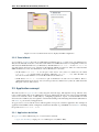
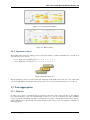
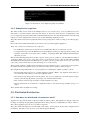
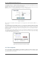
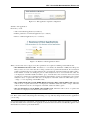
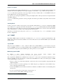
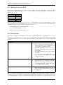
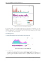
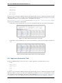
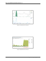
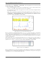
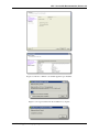
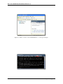
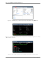
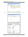
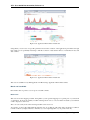
Example: A user checks out a Web page once at 16:38...
Figure 2.11: Flow example at 16:38 to 16:40
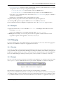
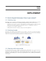
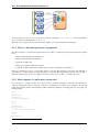
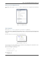
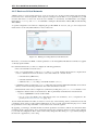
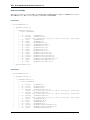
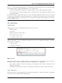
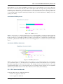
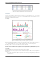
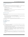
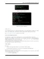
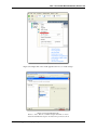
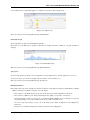
. . . and once at 16:41.
Figure 2.12: Flow example at 16:40 to 16:42
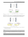
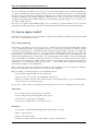
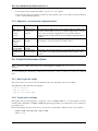
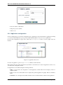
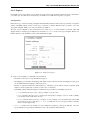
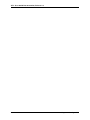
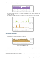
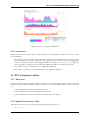
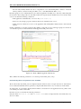
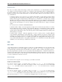
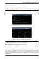
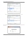
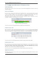
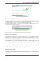
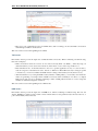
Then here is the aggregated line for both events if you query between 16:38 and 16:42:
Figure 2.13: Flow aggregation from 16:38 to 16:42
Observe that the traffic, and the packet, handshake and transaction counts have been added, and the EURT averaged. For example handshake is now 19 (12 + 7).
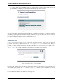
Note: Performance Vision requires a complete set of data for an aggregate level to compute its summary. This is
the reason why captured network events don’t appear right away on your probe: the probe first waits until the end
of the minimal aggregate time of 2 minutes, computes its summary, and only then is the aggregated data for these
last 2 minutes made available in the interface.
12
Chapter 2. Main terms and concepts