1
Analyzing DSC Data
1. Double click on the Microcal Inc. DSC icon to open the RawDSC window.
2. Click the Read Data button and the Import Multiple ASCII window opens.
3. Find the folder with your files in it. Then double click on the sample and
reference filenames to move them to the lower box.
4. Click OK. This puts them both on a graph in the RawDSC window. The active
plot is the one with a box around its line.
5. Click on the Subtract Reference button on the left and a dialog box opens for
choosing the data and reference filenames from drop down lists. Enter the correct
filenames and then click OK. Every point in the reference curve is subtracted
from the corresponding point in the sample curve and the result is plotted out as
filenameDSC_cp. (To view your raw data, see the Viewing Worksheet Data
section below.)
6. Now you need to normalize the data to concentration. This gets you from the
units cal/deg to cal/mole/deg and prepares your data for curve fitting later.
a.
b.
c.
d.
Click on the RawDSC window to make it active.
Click on the Normalize Concentration button. (on the left )
Enter the sample concentration and cell volume and click OK.
This moves the data to a new window called NormDATA.
7. The next thing to do is create a baseline for your data.
a. In the NormDATA window, choose Peak, then Start Baseline Session.
b. Origin plots in red the left and right linear line segments from which to
determine the baseline.
c. If you accept these default line segments, you may proceed to connect
them in one of six ways. (These are listed under Baseline in the tool bar.
See a description of each in Baseline Options below.) Choose one of these
options or opt to draw your own baseline manually. For a single
transition, the Progress Baseline option approximates the total heat change
due to the transition.
d. Click OK in the toolbar to accept this baseline. Origin then asks if you
want to subtract this baseline. Click Yes and the program exits the
baseline session.
8. Now you can fit your data. Double click on the peak to start the fitting routine,
then click on DSC in the toolbar. There are four possible models in the software
and you want to get the best possible fit using the simplest model, so try Model 1
first and see how good the fit looks. (Tm very close to the peak value and the chi-
squared stops changing.) If you think the fit could be better, try a more complex
model and see if that improves things.
The models and parameters involved are:
Model
Model 1:
Model 2:
Model 3:
Model 4:
Parameters
2 State
Non 2 State
2 State w/dCp
Dissoc w/dCp
Tm , H
Tm , H, Hv
Tm , H, Cp , BL0, BL1
Tm , H, Cp , BL0, BL1, n
For a brief description of the four models, see pp. 17-21 of the Origin Tutorial
Guide. For more details about curve fitting, see Lesson 5 in the Guide, starting on
p. 45.
9.
If you want to integrate your data (to get the integration range, temperature
range, area, thermal midpoint, and width of curve in degrees C at half height), see
Lesson 3 (p.29) in the Guide. To set the integration range, you will need to use
the Data Selector tool whose use is described in Lesson 2 (p.23) in the Guide.
Viewing Worksheet Data
If you want to see the numeric values of your raw data, they're in a worksheet associated
with your data file and the worksheet's name will be: filenamedsc_cp. The Y axis data
is Cp (heat capacity).
•
To open the worksheet, have your data loaded into the RawDSC window. From
Data on the toolbar, choose your filename at the bottom of the menu and the Plot
Details dialog box will open.
•
Click on the Worksheet button on the right and the raw data will be displayed
with temperature in the X axis column and heat capacity (Cp) in the Y.
•
To reconfigure the worksheet or extract (move) data to another worksheet, see the
Origin User's Manual, p.70. If you manipulate the data in the worksheet, it will
be altered permanently and your original raw data will be lost.
Baseline Options
There are two ways to adjust the automatically determined linear segments. One is to
refit them and the other is to move them with the cursor. See p. 39 in the Origin Tutorial
Guide for details.
Progress Baseline
reflects the progress of the reaction by checking the fraction of the total area completed at
that temperature – approximates molar heat capacity of the mixture using only slope and
intercept of the linear segments – you can limit what part of the data it integrates (using
the Data Selector tool)
Linear Connect
directly connects the end points of the two segments
Cubic Connect
connects end points of segments but also uses the slope and makes the connection a cubic
polynomial
Step at Peak
linear connect with step directly under the peak
Step at Half Area
linear connect with step at the position of half the integrated area
Move Baseline by Cursor
Choose one of the above baseline creation commands.
Then choose Move Baseline by Cursor.
Get 12 points you can move vertically.
Then set changes with Return.
This gives you a spline connection.
Cursor Draw Baseline (no linear segments determined)
Manually draw your own baseline using commands from the Peak menu.
•
•
•
•
•
Cursor Draw Baseline allows you to place as many points as you wish. They'll be
connected with a straight line.
Set the baseline with the Pointer tool. (p. 43 of the Guide)
Fine-tune with Adjust Baseline. (p. 43)
Change the connect type through Plot Details. (p. 44)
Subtract baseline. (p. 44)
Other Useful Details
Lesson 8 (p. 59) in the Origin Tutorial Guide describes:
•
•
•
•
Chi-squared Minimization
Response Time post-scan adjustments
Line Types for Fit Curves
Inserting an Origin graph into Word
Appendices
All equations used for data analysis are described in detail starting on p. 65 of the Origin
Tutorial Guide.
Updated: 5/23/12