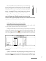
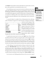
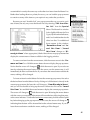
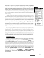
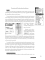
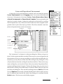
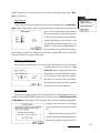
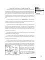
1
AppleCORE
Version 8
User Guide
updated August. 1999
AppleCORE
Version 8
Revised August 1999
User Guide
A logging system for the recording and display
of stratigraphic data
Designed and Programmed
for the Macintosh™ by
Mike Ranger
Limits on Warranty and Liability
The software and the documentation are licensed to the licensee without any
warranty express or implied including, without limitation, any implied warranties
of merchantable quality and fitness for a particular purpose, unless expressly
included in a license agreement. Due to the diversity of conditions under which
the software may be used, no warranty of fitness for a particular purpose is offered
or implied.
Michael J. Ranger shall not be liable for any loss or damage howsoever caused,
including without limitation indirect or consequential loss or damage arising out
of or in connection with the use or performance of the software or the
documentation.
COPYRIGHT
This manual and the software described in it are copyrighted with all rights
reserved. Under copyright laws, neither this manual nor the software may be copied
in whole or in part without the written permission of Michael J. Ranger, except to
make a backup copy. This exception does not allow copies to be made for others,
whether or not sold. Under the law, copying includes translating to another
language. The software may not be altered or disassembled in any way.
©1999, Dr. Michael J. Ranger
808 West Chestermere Drive,
Chestermere, Alberta
CANADA T1X 1B6
tel: 1 403 235-2712
fax: 1 403 235-2723
e-mail: [email protected]
Apple is a trademark of Apple Computer, Inc.
Macintosh is a trademark licensed to Apple Computer, Inc.
Table of Contents
Introduction ....................................................................................................
How this manual is organized ..............................................................
Installing AppleCORE .............................................................................
QuickStart .........................................................................................................
The Windows ..................................................................................................
The Log Header Window .......................................................................
The Box Tally Dialog .........................................................................
The Box Depths Dialog ......................................................................
The Data Entry Window ..........................................................................
The Strip Log Window ............................................................................
Modifying the Column Order and Column Width ........................
The Image Viewer Window ......................................................................
The Menu Descriptions .................................................................................
The File Menu ...........................................................................................
Initiating a New Log ...........................................................................
Opening and Closing an Existing File .............................................
Saving a File to Disk ...........................................................................
Importing ASCII Files ........................................................................
Exporting an ASCII File .....................................................................
Importing X-Y data .............................................................................
Importing Digital Images ...................................................................
Page Setup .............................................................................................
Printing .................................................................................................
Quitting the Program .........................................................................
The Edit Menu ...........................................................................................
Inserting and Deleting Intervals ......................................................
The Special Menu .....................................................................................
Options ..................................................................................................
Editing Lithologies ..............................................................................
Editing Icons .........................................................................................
Pore Types, Hydrocarbon Indicators, Core Disturbance ........
Caution ............................................................................................
Editing the Sample Types ..................................................................
Facies Colours.........................................................................................
Custom Files .........................................................................................
Photo, Sample and Remarks Files ...................................................
AutoSave ..............................................................................................
AutoSave Preferences ........................................................................
The Logging Menu ...................................................................................
Clastic and Carbonate Lithology Menu Items ................................
Interbedded Lithology ..................................................................
Lost Core ..........................................................................................
Box Space .........................................................................................
Recording Lithology with the Ternary Diagram ....................
1
1
2
4
8
9
11
11
13
16
17
19
20
21
21
23
24
25
27
28
29
30
33
34
35
36
37
37
41
44
45
47
48
50
51
54
55
57
58
58
59
60
60
61
Erasing Lithologies ........................................................................
Facies Contacts ...............................................................................
% Clay ..............................................................................................
Logging with Graphic “Icons” ...........................................................
The Ichnofossil Palette .................................................................
Grain Size, Texture .............................................................................
Porosity and Hydrocarbon Indicators ..............................................
Porosity ............................................................................................
Hydrocarbon Indicators ................................................................
Sorting/Roundness ............................................................................
Rock Colour ...........................................................................................
Hard Rock Structures ........................................................................
Post-depositional Features ................................................................
Diagenesis and Fractures .............................................................
Lithification ....................................................................................
Core Disturbance ...........................................................................
Oriented Core ................................................................................
Facies and Depositional Environment ...........................................
Stratigraphy ........................................................................................
Text Entry Menu Items ......................................................................
Working with Depth Markers ..........................................................
Recording Thin Sections ....................................................................
The Drafting Menu ...................................................................................
Specifying the Strip Log Format .......................................................
Scale ..................................................................................................
Litho Column: Profile ...................................................................
Lost Core ..........................................................................................
Contacts ...........................................................................................
Legend ..............................................................................................
Header Options ..............................................................................
Page Margins ..................................................................................
Drafting Partial Intervals .............................................................
Export Options ..............................................................................
Colour ..............................................................................................
Plotting Data Columns .................................................................
Symbol (Icon) Items ......................................................................
XY Plots ............................................................................................
Cumulative Plots ...........................................................................
Porosity ............................................................................................
Remarks ..........................................................................................
Facies/Environment and Stratigraphy ......................................
Modifying the Strip Log Columns ..............................................
Drafting the Strip Log .........................................................................
Saving the Strip Log as a Graphic Image File ................................
Page Breaks ...........................................................................................
Using Format Files ..............................................................................
62
63
63
65
66
68
69
69
69
71
72
73
75
75
75
75
76
77
79
81
83
85
86
86
86
87
89
89
90
90
91
91
91
92
92
93
95
97
98
98
99
99
101
103
105
106
The Search Menu ......................................................................................
Navigating Through the Schematic Data .........................................
The Window Menu ..................................................................................
Recording Hard Rock Data ...........................................................................
The Hard Rock Lithology Palette ............................................................
Hard Rock Description Dialogs ...............................................................
Mineral Component Lists ...................................................................
Mineral Selection Dialog ....................................................................
Mineral Description Dialog ...............................................................
Texture/Fabric Dialog ........................................................................
Secondary Alteration Dialog .............................................................
Alteration Products Dialog ................................................................
Voids description Dialog ....................................................................
Using the Key to Determine Rock Name ........................................
Using the Key to Determine Rock Name ........................................
Recording Hard Rock Thin Section .........................................................
107
107
108
109
109
109
112
113
115
116
117
118
119
120
120
123
INTRODUCTION
AppleCORE is a Macintosh program designed to be used in the lab while examining subsurface core. It can also be configured for logging of outcrop data or
most other kinds of lithologic data. The program allows the direct collection of descriptive geological data in a fast, standardised manner, and translates the data
into a finished strip log that is suitable for publication in reports or academic journals. The data can also be exported in a simple format to be read by other applications such as spreadsheets or for transfer to a proprietary database.
The raw data are saved to, and retrieved from, a floppy disk or hard drive and
may be redrafted and displayed at any time using different display options. The
geologist or technician is therefore relieved of the need to record notes or rough
strip logs that require tedious and time-consuming final drafting into a finished
display log.
The finished strip log can be viewed and interpreted immediately after (or even
during) the logging process. The strip log can be printed out either in high resolution on a Laser printer such as Apple’s LaserWriter or as a continuous strip log in
colour or black and white on a dot matrix printer such as Apple’s ImageWriter, or
on any other compatible printer. The strip log can also be saved as a QuickDraw
“PICT” file, which can be imported into many Macintosh graphics applications,
CAD and desktop publishing programs. This feature allows full editing and enhancement of the drafted strip log to personal taste on a variety of different commercial software.
The Logging menus also act as a “prompt” while logging, which encourages a
thorough and systematic approach to a basically interpretive and deductive endeavour. AppleCORE utilises the standard Macintosh graphic interface of icons
and pull-down menus, and relies almost totally on the mouse for data input. The
keyboard is used only for text entry.
How this Manual is Organized
Those users who are already familiar with the Macintosh can quickly get started
using AppleCORE by reading through the QuickStart notes in the first few pages
of this manual, as well as the detailed descriptions of AppleCORE’s three main
windows that follow. Comprehensive explanations of all of AppleCORE’s functions are organized under the same headings as the program’s menu bar at the
top of the screen. Each item under these headings is then described in the vertical
1
order in which they appear when the menu is pulled down. The pulled down menu
is displayed at the top edge of each page, with the described item inverted. Thus
you can quickly find information on any item in a particular menu by flipping
through the pages of the manual while keeping your eye on the upper edge of the
pages.
The appendix volume contains important information on the internal code numbers that AppleCORE uses for its data. These code numbers are used when the data
are downloaded as an ASCII file. If you require use of the exported ASCII file, its
format is also described in detail in the Appendix.
Installing AppleCORE
There is no copy protection on AppleCORE. To install it on a hard drive, simply drag it from the floppy disk or CD to your hard drive icon. AppleCORE may
be compressed. To decompress, double-click on the hard drive version and follow
the instructions. Keep the original disk as your backup copy.
Make sure AppleCORE is unlocked before using, otherwise any new icons or
lithology patterns that you create will not be saved (you will get a warning). To
check if it is locked, quit AppleCORE, and “select” it by clicking once on its icon.
Then, from the “File” item in the system menu bar, select “Get Info”. The lock
button is in the lower left of this window. You can toggle it on or off by clicking on
it. Make sure it is off.
In the Get Info window you can also assign
AppleCORE’s memory requirements. Select
“Show: Memory”. The default preferred size is
3000K (3 megabytes). This should be adequate
for most work. But if you get a message that
memory is low when running AppleCORE, you
can assign more memory by increasing the preferred size to, for instance, 4000K. You can only
make changes in the Get Info window when
AppleCORE is not running.
Once you are comfortable using the mouse, you will probably want to set the
mouse tracking to the fastest available i.e. a minimum movement of the mouse
results in the maximum movement of the cursor on the screen. Set this in the Mouse
2
control in the Control Panel under the
menu.
If your Macintosh supports colour, the lithology palettes and the core schematic
will be displayed in colour. Colour causes the lithologies to stand out and adds
another dimension to the logging process, making it even more intuitive. Set your
system colours from the Monitors control. (Choose Control Panels from the
menu in the menu bar.) AppleCORE displays colour best with your monitor configured for 8 bit colour or better. To get this, choose “256” colours (or greater) from
the Monitors dialog. If the shale lithologies are displayed as grays instead of
greens on your colour monitor, you probably have your monitor configured for 4
bit colour allowing only 16 different colours. Most colour systems now have enough
VRAM to allow you to display a minimum of 256 colours, allowing AppleCORE
to operate with its full range of default colours.
3
Up and Running Quickly
QuickStart
If you are already familiar with the Macintosh these QuickStart notes will get
you up and running with AppleCORE without having to read through the entire
user manual.
— AppleCORE requires Macintosh System 7 or 8, and requires a PPC processor
— When creating a new log you will have to choose between “Core mode” or
“Outcrop mode”. The main difference between the two is that in Core mode,
you must record the core and box numbers before proceeding. This allows the
program to keep track of the core boxes and their depths automatically as you
record data. In Outcrop mode you can record data stratigraphically up or down
without limit.
— The first window that appears when creating a new log or opening an existing
log is the header window. Before the program will allow you to enter any sedimentological data in Core mode, you must first click on the Box Tally button
and enter the number of boxes for each core. This information may be changed
at a later stage. It is not necessary to enter the Box depths at this stage, however you will not be able to draft the log without the depth information. Once
Box Tally information is entered, most of the menu items become activated.
— Before you start recording sedimentological data (in core mode) you have the
option of showing the core box schematic with one or two columns to mimic
the actual core box. This option is accessed through the Options item under
the Special menu. (The options for more than 2 columns per box are not yet
available)
— Automatic Depth Increments (in the Box Depths dialog) will automatically
increment succeeding or preceding boxes as long as a top and bottom depth
are recorded for the box showing. The incrementation occurs as you click uphole or downhole and as long as both the top and bottom depths of the succeeding or preceding box are both 0.0.
— Bring up the Data Entry Window by choosing any item from the Logging menu.
Record data by dragging the mouse over the desired interval or “double click-
4
ing” in an interval. Double clicking in an empty box schematic fills that box
with the data item. Double clicking or dragging over an interval that already
contains data will substitute the new data for the existing data.
QuickStart
— An effective way to collect data is to first record all the lithologic data as your
basic facies intervals. Then “double click” all the other information into these
intervals.
— The top and bottom of a core column are assumed to be continuous facies intervals with the preceding or succeeding intervals if the lithologies are the same.
If a break is desired at the column boundary, place a facies contact at the boundary by clicking the selected contact near the boundary.
— Place a facies contact by first choosing one from the pop-up menu. Switch on
the Facies Contact button if it is not already on. Then place the contact by
clicking once in the core schematic on or near the facies boundary. You can
only place contacts at the base of a recorded facies interval. To place a boundary within an existing interval, first divide that interval by dragging the mouse
from the desired boundary position to either end of the existing interval. Then
click the contact into the new boundary.
— All of the available palettes are accessed by clicking on the small icons at the
lower left of the lithology menu to bring up pages one to four of the lithology
items. A total of 64 lithologies are available for each of clastics and carbonates,
and these may all be customised from the “Special” menu, or by simply double-clicking on their buttons, which opens the edit dialog window.
— To record interbedded lithologies: choose the primary lithology with “interbedded” turned off. Then click “interbedded” on and select the secondary lithology. The “%” and “bedding thickness” are pop-up menus, and are recorded
along with the interbedded lithology.
— Two palettes of icons are available for each of the Structures, Accessories, Trace
Fossils, and Fossils. Click the double arrow button at the lower left to alternate between the two palettes. However, many more icon items are available
from a “Master List” from which you can load the palettes. Call up the master
list to customise an icon item and alter the working palette by “double clicking” on the icon position in the palette. You can also call up the master list and
customise the icons from the Special menu, but you can only alter your working palette by the double click method.
5
— Many data palettes have an “erase” button. All other data items can be erased
by dragging or clicking with the command key (
) held down.
QuickStart
— If you find that too many icons are cluttering up the schematic column making
it difficult to place new items, you can temporarily hide all icons except those
from the active menu by holding down the option key.
— Pore Types and Hydrocarbon Indicators are selected from “pop-up” menus.
Customise the items and the appearance of the pop-up menu from the Special
menu.
— Move uphole and downhole quickly from the keyboard by using the cursor up
(↑) and cursor down (↓) keys. With the extended keyboard, the page up and
page down keys do the same thing. The home and end keys take you to the
top and the base respectively.
— When recording Facies and Depositional Environments, or Stratigraphy, whatever is in the text edit box with the blinking cursor is the text that is recorded.
The scrolling menus provide a selection of prerecorded items. Load any of these
into the text edit box by clicking on the item. And anything in the text edit box
can be uploaded to the prerecorded list using the appropriate control buttons.
All items on the prerecorded lists of Facies and Depositional Environments can
be colorised to make identification easier on the drafted strip log. To colorise
an item, select it by clicking on it, and then choose “Colorise Selected
Facies” from the Special menu.
— To record text remarks on the log, choose Text from the Logging menu. The
cursor will change to a pencil when moved over the core schematic. Click at
the appropriate depth, and a text editing window will appear. When the window is closed, an icon of a note pad will appear on the core schematic to indicate the presence of the text item. Click on this icon at any time to re-display
the text window. Photo, Sample and Label work in a similar way.
— The strip log may be drafted up at any time as long as depths are recorded for
all intervals. The program will inform you of any discrepancies in the depths
that may prevent the log being drafted. To draft in colour, turn on the color
button in the “Set up Format...” dialog under the Drafting menu. The strip log
format can be saved as a “Format File”, and can then be “Applied” to other
logs, for example to replicate a complex format on a multi-well project.
6
— The strip log must be drafted before you print. The Print command under the
File menu will be dimmed until the log is drafted. To print in color, the log must
be drafted in color, and “color” must be chosen in the Print dialog.
QuickStart
— If the drafted strip log is saved as a PICT file (choose under the Drafting menu),
the graphic image can then be opened by many graphic and drafting programs
such as Canvas or MacDraw Pro for further enhancement.
— IF YOUR SYSTEM CRASHES while AppleCORE is open, you have a good
chance of recovering most of your work if you have left “AutoSave” turned
on (under the Special menu). Restart your computer and look immediately
in the Trash. There should be a folder there entitled “Rescued Items...” which
will contain the last file you worked on. Its title will be “Recovered...” followed
by the name of the file or “Untitled”. The interval between backups can be set
by selecting “AutoSave Preferences” under the “Special” menu. An application may crash by quitting “unexpectedly”, but otherwise still leave the
system running. If this happens while running AppleCORE, you can recover
your file only by restarting the Mac (choose Restart from the Special menu
of the system menu bar). After the restart, check the trash for your file.
7
The Windows
AppleCORE uses four main windows for the collection and display of data:
The Log Header and the Data Entry windows are used for data entry, and the Strip
Log window is used for data display. The Image Viewer Window allows display
of digital images to aid in logging. Each of the windows can be accessed from the
“Window” item in the menu bar.
The Log Header window is used to enter descriptive and configuration data
about the well or stratigraphic section. This is typically information that you would
expect to see on the strip log header, hence the name. In “Core” configuration there
are two buttons in the lower right of this window labelled the Box Tally button
and the Box Depths button, which are used to record the number of cores and
the number of boxes in each core as well as their depths. The Log Header window disappears when not in use.
The Data Entry window is used to graphically record the descriptive data. It
has a number of different “palettes” and therefore it changes its appearance somewhat depending on the type of data that is being recorded. The different data
palettes are selected from the “Logging” item in the menu bar. When you choose
one of the logging palettes, the Data Entry window will be made the frontmost
window if it isn’t already. You can change the position of the Data Entry window on the screen but you cannot alter its size.
The Strip Log window is a scrolling window that displays the drafted strip
log. No data can be entered from the Strip Log window. The Strip Log window
can be resized and its position on the screen may be moved as desired.
The fourth window, the Image Viewer window, is a scrolling window that
displays digital images imported from several different formats. The digital image can be rotated and scaled, and the Image Viewer window can be resized and
its position on the screen may be moved as desired.
8
The Log Header Window
This window opens when a new file is created or when an existing file is opened.
The window contains a number of text entry fields that are used to produce a header
for the strip log, as follows:
-the well name (maximum 255 characters);
-the location in township - range format. Note: when entering the meridian, it
is not necessary to include the letter “w” as in “w4” (west of the 4th meridian),
since this is automatically included on the drafted strip log title. A general area
(“other”: maximum 255 characters) is provided for locations that are not in the
township survey system;
-the present date: the date is filled in automatically with the present date from
the computer’s clock, however this may be edited if required (maximum 50 characters);
-the name of the person logging the data (maximum 255 characters);
- the ground elevation and KB elevation.
-remarks: there is no limit to the amount of text that can be entered as “header
9
remarks”. If you type more than can be displayed, use the vertical scrolling control at the right hand side to scroll through the text entry box. Note that these remarks are (optionally) plotted only in the strip log header, and are not the same as
the depth related remarks you may record while logging core.
Note also that if you choose ODP (Ocean Drilling Program) configuration, the
Log Header window will have a slightly different appearance and terminology.
Also, the Remarks box is not accessible to the user and will be hidden.
As well as the preceding header data, you must also configure the program
for metric or imperial units. The desired choice is made by clicking on the appropriate “radio” button, either feet or meters. This lets AppleCORE know which units
the input depths are measured in. Once you have set this button, there should be
no reason to ever change it for that file. Changing it will NOT do any conversions,
or change the data in any way. When drafting, the strip log can optionally be plotted in either meters or feet, and in that operation AppleCORE will do the appropriate conversion for you. However the units of the original depths need never be
changed. The “original depths” are those entered in the Box Depths dialog described
below.
When logging in “Core” configuration (see the section: “Initiating a New Log”),
information must be recorded that indicates to the program the sequence of cores
and boxes. Before this basic information is provided, most of the menu items will
10
be dimmed, and logging cannot proceed. (In “Outcrop” configuration, this information is meaningless, and logging may proceed immediately.) The Log Header
window includes two buttons that are used to enter the core and box information:
the Box Tally and the Box Depths buttons.
The Box Tally Dialog
The “Box Tally” button
opens a dialog window that
prompts the user to enter the
number of boxes in each core.
Selecting uphole or downhole
Text Entry Box
displays the core numbers in
sequence, and the number of boxes is entered in the text entry area. The text entry
area will accept 0 as the number of boxes, however core data will not be accepted
for any cores with 0 boxes. You will hear a beep if anything other than a numeric
character is entered.
The number of boxes in any core can be altered at any time in the program, but
be aware that reducing the number of boxes will cause the loss of all data from the
deleted boxes. Boxes are added to and deleted from the base of a core so that, for
instance, reducing the number of boxes in a core from 5 to 3 will destroy boxes 5
and 4. (A warning is displayed before you are permitted to delete boxes).
The Box Depths Dialog
The “Box Depths” button
opens another dialog window
that prompts the user to enter
the depth of the top and base for
each box. The unit of measure
Text Entry Boxes
(feet or meters) must be that se-
lected in the Log Header window. Once the top depth and the base depth of the
first box are entered, selecting downhole will display the next box in sequence, and
the top depth is automatically recorded as the base of the previous box. (This depth
may be changed if there is a gap in the core recovery). Depths may increase upwards or downwards, and negative numbers will be accepted. Any depths that
are not entered are recorded as 0.0 This will not prevent the user from recording
11
and saving lithologic data, however the strip log cannot be drafted until all the
depths are entered.
After the depths are entered for each box, there is normally little need for the
user to be further concerned with these depths while logging the core. Entering
the depths accurately is a necessary and important step since the strip log is drafted and scaled based on these data. Any error in these depths will cause anomalies
to appear on the strip log. The depths may be altered and corrected at any time. If
an error is made such that the recorded depths of any boxes overlap, a warning
will be issued when you attempt to draft the strip log.
Switching on “Automatic Depth Increments” can greatly facilitate the
entry of the depths. To use this feature, enter the top and base of any box. The program computes the depth interval for that box. Now as you move sequentially up
or down through the boxes this same interval will be incremented in succeeding
boxes. The depths will not be incremented if any value has already been entered
for either the top or base of a succeeding box.
Note that there is an optional method for recording the depths. Instead of using the Box Depths dialog described here, the depths may also be entered or changed
directly in the “Data Entry” window (see the following section).
12
The Data Entry Window
The Data Entry window can display several different palettes allowing the
collection of many types of data. The data entry palettes are accessible from the
Logging menu in the main menu bar at the top of the screen. The palettes all have
two items in common:
Control Buttons
Text Editing Boxes
an interval schematic
located at the right of
the screen, and a control
box in the upper left of
the screen that contains
the core box or interval
selection controls. The
control box displays the
current core and box,
and its top and bottom
depth. The top and base
Alternate palette buttons
Lithology palette
Scale bar
Core box (Interval)
schematic
depths are displayed in
text editing boxes and
are fully editable. You may enter or change the depths from the Data Entry window as an alternative to using the Box Depths dialog from the Header Window.
The uphole and a downhole buttons allow you to step sequentially through
the recorded data intervals.
You may also use the up arrow ↑ and down arrow ↓ cursor keys on the keyboard to move through the box schematics. If you have an extended keyboard, “page
up” and “page down” will also take you sequentially through the data, and the
“home” key and “end” key will take you to the top and bottom respectively of the
core. The home and end keys duplicate the Go To Top and Go To Base items in
the Search menu.
If you are logging in “Outcrop” mode, the control box will look slightly different. Outcrop mode is a more generic configuration that does not use the core and
box model. Therefore the Box Tally and
Box Depths buttons do not exist (in the
Log Header window), and the control box
does not indicate core and box numbers. You
13
may move up or down with no limits, and depths are recorded only in the top and
base text editing areas of the control box.
The “Automatic Elevation Increments” button appears in the control
box in outcrop mode. When this button is on, AppleCORE computes the thickness
interval for the current schematic. It will then set the top and base of succeeding
schematic intervals by cumulating (or subtracting) the computed value as you move
sequentially up or down through the schematics. Automatic incrementation will
not occur if any value has already been entered for either the top or base of a
succeeding box.
Recording data from core is accomplished by entering information so that the
schematic core box graphically duplicates the actual core. You choose patterns and
symbols (icons) from the palettes by clicking on them with the mouse button. That
item becomes the curSelected item
Cursor depth
Selected item
"clicked" in place
rent
item,
and
you
record it in the core schematic using only the
mouse by clicking the
mouse button or dragging over an interval in
the schematic with the
mouse
button
held
down. As you move the
mouse over an interval
in
the
schematic,
AppleCORE will keep
Scale bar
Alternate palette button
Core box (Interval)
schematic
track of the scaled depth,
updating
it
continu-
ously. This allows you to accurately place the graphic elements. A customisable
scale bar next to the schematic may also be used to place the graphic elements. This
is useful when it is configured with divisions similar to a full scale rule placed next
to the actual core box. Most of the patterns and icons are those in common use and
should be familiar to all sedimentologists. But all graphic items can also be customised if you prefer, and you can create your own if the basic standard set is not
sufficient.
If you find that too many icons are cluttering up the schematic column, mak-
14
ing it difficult to place new items, you can temporarily hide all icons except those
from the active menu by holding down the option key on the keyboard.
As you log the data into the schematic, you are creating a graphic image of the
core. However you are also building up a numeric file of all the data items as you
log them, and it is this data that is saved when you save a file. The graphic image
that appears as the schematic is only the human interface that AppleCORE recreates every time a file is created or opened.
You will come across a several graphic interface elements repeatedly when working with the
palettes. All are standard Macintosh dialog items,
and will be familiar to those experienced with
Radio buttons
(only one at a time is on)
using the Macintosh. There are three kinds of
dialog buttons: Radio buttons and Check Box
buttons allow you to choose options; “Action”
buttons always have a consequence and perform
Check buttons
(option on or off)
a function. Note that you can click Radio and
Check Box buttons anywhere in their titles. You
don’t have to be careful about only targeting the
image of the button itself.
Besides the menus in the menu bar at the top
of the screen, AppleCORE also uses many “pop-
"Action" buttons
up” menus as a convenient way to choose items
or modifiers from a palette. Any text box that has
a “drop shadow” behind it is a pop-up menu. To show the menu, click and hold
the mouse button with the cursor over the menu box. Then move the cursor to the
desired item and release the button. The selected item becomes the current item,
and will be placed in the pop-up menu
box. If you release the button outside the
Popup menu
(box with shadow)
menu, no selection will be made and the
original item will remain the current
item.
Step-by step instructions on how to
Menu "popped up"
use each of the palettes are detailed under
the sections dealing with the Logging Menu, but you should find the graphical
logging process quite intuitive after very little practice.
15
The Strip Log Window
The Strip Log window allows the user to preview the drafted strip log produced from the recorded data. The strip log is drafted according to the format that
is created in the “Setup Format...” dialog selected under the “Drafting” item
in the menu bar. The Strip Log Window is not available under the Window menu
and you cannot print until you have drafted the data. If you change or add data,
the Strip Log window will be out of date, and you must “Redraft” to update it.
You can draft up your data at any time. You don’t have to wait until the full core
description is finished. In fact it is usually a good idea to draft up the log early in
the data collection process to see how it will appear at the desired scale. You may
find you are logging in too much detail for that scale.
The first time the Strip Log window appears, it will fill the screen. It can be
resized by clicking in the
icon in the lower right of the window and dragging
to the desired size while holding down the mouse button. To change the window’s
position on the screen, click anywhere in its title bar and drag it to the desired
position.
16
The vertical and horizontal scroll bars allow you to scroll through
scroll
arrow
the strip log if the screen is not big enough to show the entire image.
Click in the scroll arrows to move a few lines at a time, or click in the
shaded area to move a page at a time. Or you can click on the “thumbwheel” icon and drag it to a new position in the scroll bar. This will
scroll the image to the same relative position in the window.
When you print the log, the printout will look more or less the
thumbwheel
same as the drafted strip log on the computer screen. However, the
resolution of the printer is much higher than the screen, so that the printed image
typically looks much sharper than the screen image.
Modifying the Column Order and Column Widths
The data columns on the strip log may be plotted in any order, and the widths
of some (but not all) of the columns may also be adjusted.
To change the plot order, first draft the strip log. Then hold down the Shift key
and move the cursor into the column caption area at the top of the strip log. The
cursor will change to a hand icon,
and you may then click and drag the col-
umns into any desired order. The strip log will redraft in the new column order
after each drag. You must keep the Shift key depressed as you drag the columns
into position.
To change a column width, hold the Shift key down and move the cursor into
the column caption area at the top of the strip log. The cursor will change to a double
direction arrow
when positioned over a column boundary that can be adjust-
17
ed (otherwise it will appear as the hand icon). Some columns cannot be adjusted.
REMA RKS
Click and drag the column margin to the desired width. A column width is adjust-
ed from its right-hand margin. The strip log will redraft to the new column width
after each drag. You must keep the Shift key depressed as you adjust the widths.
18
The Image Viewer Window
You may display digital images to aid in recording data. The image will appear in a separate window. You may rotate the image clockwise or counterclockwise, and scale it if desired.
You will require the QuickTime extension v.3 or higher in your system folder
in order to view digital images.
AppleCORE supports the following image file formats: PICT, TIFF, GIF, JPEG/
JFIF, BMP, PNG, Targa, QuickTime Image, MacPaint, Photoshop (v. 2.5 and 3.0)
and Silicon Graphics.
19
The Menu Descriptions
To use the AppleCORE program, boot the Macintosh using System version 7
or any later version. To start the program, click twice on the AppleCORE icon, or
select it by clicking once on the icon and choosing Open from the File menu. Several seconds are required while the program sets itself up. During this time, licensing
information will appear and the “busy” wristwatch cursor will be displayed. When
the menus appear at the top of the screen, the program is ready for use. The licensing information window will disappear at the first click of the mouse button.
Menu items are selected by holding the mouse button down while the arrow
cursor is over the desired menu heading. This “pulls down” all the items under
that heading. Release the mouse button over the desired item. Disabled items are
dimmed and cannot be selected because they are inappropriate choices. Note that
most menu items are dimmed immediately on starting the program if configured
for logging core. Once Box Tally information is entered from the header window
or an existing data file is opened, most of the menu items become activated. Many
menu items may also be selected from the keyboard by holding down the command (
) key while hitting another key (i.e. a “hot key”).
The specific keyboard short-cut for each item, if one is availkeyboard shortcut
able, is listed after the item’s title in the pull-down menus.
One item under the
menu contains an AppleCORE item. “About
AppleCORE” contains copyright information and also displays the amount of RAM
memory remaining that is available to AppleCORE. This information can be useful if you have a large file open and are worried about running out of memory.
The “About AppleCORE” notice
also shows the current Custom
file (see the section: “Custom
Files”).
20
The File Menu
Initiating a New Log
To start a completely new file, select “New Log” from the menu. This opens
up a Log Header window (see section: “The Log Header Window”) whose fields
are all blank except for the present date, which is automatically initialized.
When New Log is chosen from the File menu, a dialog box will require that
you to choose a configuration: either Core or Outcrop. The Core option requires
that you enter information through the
”Box Tally” dialog (button in the log
header window) before AppleCORE will
allow you to begin logging data. This information consists of the core numbers
and the box numbers for each core. When
logging, you are then constrained to moving uphole or downhole within the core intervals. This is an advantage when logging core directly in the lab, because AppleCORE can then keep track of which
core box is being logged and display it as an exact scaled schematic. The Box
Depths information is not required before starting to record data, however the
strip log cannot be drafted until all depths are entered.
AppleCORE can also be used for logging of outcrop data. Typically one may
wish to transcribe field notes into AppleCORE format for easy drafting. Instead
of forcing you to enter the data as if it where collected from a series of drill cores,
AppleCORE can be configured to operate in a more “generic” manner by choosing the Outcrop configuration.
Unlike the Core configuration, the Outcrop configuration does not use the
Box Tally or Box Depths buttons. The data entry window may be used immediately and depths are entered directly from the Data Entry window. There is no
top or bottom limit imposed on the sequence of intervals as there is for core data.
You can go up or down the sequence entering data with no restraints. (There is
actually a finite limit on the number of intervals that can be recorded, i.e.: 500,000
up and 500,000 down.) In Outcrop mode the core box schematic is displayed as
a single column, representing the interval given by the top and base elevations.
The interval can represent any length, and need not be a constant interval up and
down the succession. You could, for instance, let each schematic interval repre-
21
sent a single described facies interval in your stratigraphic succession. When the
strip log is drafted, all the intervals will be scaled to the designated log scale.
In Outcrop mode, other cosmetic items such as some menu titles are changed
from core nomenclature to simple stratigraphic references. For instance, the uphole and downhole buttons become simply “up” and “down”. The data entry
palettes may also have a slightly different appearance in outcrop configuration:
The Lost Core item becomes “Covered Interval”, while the “Empty Box Space” item
is removed as irrelevant. Core and box numbers are, of course, not displayed. Instead the space is occupied by the automatic elevation increment check box. If this
is clicked on, elevations are incremented by a constant thickness as described in
the section: “The Log Header Window”.
When transcribing old written core descriptions into an AppleCORE file, some
users prefer entering the data in the generic “Outcrop” mode, especially if core
and box information has not been recorded in the notes. In this case, each interval
schematic can represent a recorded facies interval with appropriate top and base
depths.
If an existing file is opened, its configuration, Core or Outcrop, is the configuration that was chosen when the file was first created.
22
Opening and Closing an Existing File
To open an existing file, select Open Log. A dialog window will appear, which
allows the user to browse through the hierarchy of files on any hard disk or removable disk mounted on the system. Only AppleCORE files will be displayed.
Open the desired file by clicking twice on it or by clicking once to select it and then
choosing the “Open” button. While the file is read into memory the watch cursor
is displayed. The Log Header window will then be displayed with all previously
recorded header information for this file.
You can also open a file by simply double-clicking on its icon from the Macintosh desktop. This will start the AppleCORE program if necessary and immediately load the file. If you select “Open Log” while another log is already open,
the open log will automatically be closed before the new log is opened.
Opening an existing file will configure the arrangement of items on the palettes as they existed when that file was last saved. Furthermore the strip log format and the page setup format will be restored to the configuration that existed
when the file was last saved.
Note that the icon graphic images are not saved in the data files. Only the reference “ASCII” numbers for each variety of data are saved. If the icon images have
been changed in your copy of AppleCORE, the recorded icon items will be displayed with the new images. (See the warning in the section: “Custom Files” concerning customising the icons and lithologies)
To Close a file, choose “Close Log” from the File menu. If the file has had
changes made to it, including changes to the strip log format, a dialog will appear,
reminding you to save the changes.
If you have opened a file created with
an old version of AppleCORE,
changes may have been made to the
file as it was automatically updated, and even if you have not manually made any
changes to the file, a dialog will appear asking if you wish to save changes. If you
choose to save the changes, the file will be saved in the updated format, which
may not then be compatible by the earlier version of the AppleCORE. (In such cases
you may want to save the file as a different name, leaving the original unaltered.
See following pages regarding saving files.)
23
Saving a File to Disk
As you log your core, you are creating a data file in RAM. That data is not permanent until it is saved to disk. When finished recording data, select Save from
the menu to load it to a disk. If this is a new log, you will be asked to provide a
name for the file. If you have simply made changes to an existing log, these changes will immediately be saved.
It advisable to also save your work frequently while logging, especially if unfamiliar with the program or the Macintosh. A power failure or an unexpected
system error could result in the loss of all the data recorded since the last “Save”.
If you open a data file, make changes to it, and then decide that you would like
to keep the original data file intact, select “Save As...” from the menu. A dialog
window will ask you to provide a new name and the altered file will be saved as a
separate document leaving the original file intact.
24
Importing ASCII Files
AppleCORE’s normal data files are stored as binary machine code and are not
easily transferred to other platforms. However, AppleCORE can also read and write
data files in a generic text format known as ASCII code. These ASCII files can be
opened by all word processing and spreadsheet programs, and are therefore readable in plain English. These files can also be easily transferred to DOS /Windows
environments. Using this vehicle, AppleCORE files can be downloaded for transfer to other databases, or for input to statistical packages, for example. Or you may
have existing lithologic data in a specific format that you wish to import into
AppleCORE to draft up. The ASCII file provides the bridge to accomplish this.
The AppleCORE ASCII data file is a very simple format consisting of interval
depths and code numbers representing the various data items. A full description
of the ASCII file format can be found in the Appendix to this manual.
To import an ASCII file choose “Import ASCII File...” from the File menu.
This in effect is the same as choosing “Open Log...” except that the data are stored
in a different format. When the ASCII file is read in, its data are converted to the
regular AppleCORE internal format, with the title “Untitled”. To save the file to
disk as a regular AppleCORE file simply choose Save from the menu, and a dialog will ask you to give the file a name. You should give it a name that is different
from the ASCII file.
The ASCII file may contain some optional data records that provide information about the well that is normally entered in the Header
Window. But it may also contain
records
that
tell
AppleCORE how to configure
itself for this particular data
set. Although there are defaults for most of these items if
they are not found in the ASCII file, a dialog box may appear prompting the user for more information.
AppleCORE will also check the ASCII file for some errors or inconsistencies in
25
the data. If errors are found, a dialog box will appear giving the user the choice of
skipping the problem data and continuing, or cancelling the import altogether. The
dialog will also show the nature of the problem, and approximately
where
it
occurred. Note that although
the ASCII file format is relatively simple and has few restrictions, it is not possible to
anticipate all possible errors
in the data, and some files, if formatted incorrectly, may not read properly or may
simply crash the program! Technical information regarding the ASCII files is given in the Appendix to this manual.
26
Exporting an ASCII file
To create an ASCII file choose “Export as ASCII file...” from the File menu.
This creates a data file in a simple format that can be opened by any word processor and read in plain English. A dialog box will first be displayed asking if you
wish to have box and core numbers included in the file,
and whether you want the depths listed in feet or meters. If you have recorded Depth Markers, you will also
have the option of correcting all the depths to the marker depths. The exported data file consists of a list of interval depths and codes that represent the various data items that have been logged.
The ASCII file can then be used to transfer data to other programs or can be reformatted for uploading to a data base.
See the previous section “Importing ASCII Files” and the Appendix for more
information about the ASCII files. Following is an short example of what an ASCII
file would look like opened with a word processor.
LTH 2406.00 2407.00 1295 999 100 999 999 999
LTH 2407.00 2408.00 1295 999 100 999 999 999
LTH 2420.69 2421.00 999 999 100 999 999 999
LTH 2421.00 2421.17 999 999 100 999 999 999
LTH 2421.17 2421.75 1286 999 100 999 999 392
LTH 2421.75 2422.00 1286 999 100 999 999 999
LTH 2422.00 2423.00 1286 999 100 999 999 999
LTH 2423.00 2424.00 1286 999 100 999 999 999
PHY 2421.28 206
ACC 2421.33 251
ACC 2421.73 251
ACC 2421.80 251
PHY 2421.92 208
PHY 2422.19 202
ACC 2422.31 251
PHY 2422.45 208
PHY 2422.63 216
PHY 2423.40 202
PHY 2423.52 216
ACC 2423.63 251
PHY 2423.79 208
GRS 2421.00 2421.17 6 999
GRS 2421.17 2421.19 1 999
GRS 2421.19 2421.75 1 999
GRS 2421.75 2421.96 2 999
GRS 2421.96 2422.00 3 999
TXT 2421.88 342
Unit 5 probably consists of abundant small-scale coarsening-upward cycles of low angle cross laminated sandstone with truncation surfaces defining sets <50cm thick. Laminae are marked by dark, organic material; possibly finely comminuted plant debris. Burrowing exceedingly rare although unslabbed nature of core makes
determination difficult.
*Note that the word processor has added line returns to the text to fit on the screen.
On the raw ASCII file, line returns are placed only at the end of the records.
27
Importing X-Y Data
AppleCORE can import lists of data for plotting as a line graph in a separate
column on the strip log. Such data should consist of a set of depth values and a
variable to plot. Examples are readings from a Gamma Ray log or perhaps porosity measurements from a core analysis. Eight different sets of data can be imported for a log, and can be plotted in any of four tracks with two curves per track, and
annotated with appropriate scales and titles. The raw data should be in the form
of an ASCII “TEXT” file where data fields are delimited by spaces and/or tabs (commas are not acceptable). Alphabetic characters, blank lines and values of -99999.9
or less are read as null data fields, and will cause a break in the plotted curve. If
there are non-numeric data on any lines at the top of the file, AppleCORE will skip
those lines until it finds the first row of all-numeric values. All Macintosh and
Windows spreadsheets and word processors can save data in ASCII format (TEXT
or .txt format).
The raw data file can consist of any number of data columns and data rows.
When importing the data, a dialog window will list all the data columns in the file
and allow you to choose which to import. Only one column of variables (along with
its depths) can be imported at a time, and the dialog will prompt you to indicate
which data column is the depth and which is the variable.
First (numeric) Data Line
feet
API units
1505.0
39.5
1505.5
42.3
1506.0
63.5
1506.5
87.5
1507.0
108.9
1507.5
131.1
1508.0
154.2
1508.5
154.2
1509.0
156.5
1509.5
179.2
1510.0
183.3
1510.5
185.6
1511.0
185.2
1511.5
160.8
28
Importing Digital Images
AppleCORE can display digital images in a separate window to aid in logging.
The image may be rotated in 90° increments clockwise or counterclockwise, and
scale it if desired.
You will require the QuickTime extension v.3 or higher in your System folder in order to use the digital image viewer.
AppleCORE supports the following image file formats: PICT, TIFF, GIF,
JPEG/JFIF, BMP, PNG, Targa, QuickTime Image, MacPaint, Photoshop (v. 2.5 and
3.0) and Silicon Graphics, as well as Kodak photo CD’s. You could for example,
open another AppleCORE strip log that you had previously saved as a PICT file
in order to refer to it while logging. At present AppleCORE does not save or print
digital images.
29
Page Setup...
Selecting “Page Setup ...” produces a dialog box that is specific to the printer you have chosen. (To choose a printer, select “Chooser” under the
menu).
The dialog box allows you to set up
the page specifications. Shown here
is the standard dialog box for the
Apple LaserWriter. In north America, U.S. Letter size in a vertical orientation is the default option. You
can reduce the image up to 25% of
the original size or enlarge the image up to 400% of the original size on the LaserWriter. Don't forget that if you choose
to reduce or enlarge the image, the scale you selected for your drafted strip log
will be similarly effected. When reducing or enlarging on the Apple LaserWriter
the best results will usually be obtained at increments of 25%.
Page Setup also has another critical function. It tells AppleCORE the size of
the printer page, -information that may be used to format the strip log. If you change
printers, you should select Page Setup from the menu and then redraft the strip
log. Select Page Setup even if you do not wish to make any changes to the page
orientation. Simply open it and then close it again. If the new printer has a different page size, AppleCORE will then prompt you to redraft the strip log. It will not
be necessary to call Page Setup again unless you wish to change page size or
orientation.
As a default, AppleCORE tries to fit the width of the strip log on a single page.
It does this by adjusting the width of the remarks column. However, there are built
in limits. If the remarks column would be excessively wide, only part of the page
width is used. If the column would be too narrow, the image is extended laterally
onto a second page, and will have to be spliced. To avoid splicing in such cases,
try changing the default page orientation from portrait
to landscape
orientation.
You may also adjust the width of many (but not all) of the strip log columns in
order to optimise the space on a printed page. To change a column width, hold
the Shift key down and move the cursor into the column caption area at the top of
30
the strip log. The cursor will change to a double direction arrow
when posi-
tioned over a column boundary that can be adjusted. Click and drag the column
margin to the desired width. A column width is adjusted from its right-hand margin.
If a log printout has part of its graphic truncated and lost at page edges, this is
a sign that AppleCORE is using a page size that is incorrect for that printer. To
cure this, simply open and close the Page Setup dialog. Then redraft the strip
log and try printing again. (This procedure applies to all Macintosh applications.)
The Page Setup dialog may have an “Options” button. Any of the options
may be specified, however
“Precision Bitmap Alignment” will reduce your image
by 4%, thereby changing the
scale that was specified for your
drafted strip log. Also, choosing “Larger Print Area” has
been known to make manual paper feeding difficult, possibly causing a paper jam
alert.
The Page Setup dialog for the dot matrix Apple ImageWriter is shown here.
The preset option in north
America is vertically oriented
U.S. letter size. Normally you
will also want to click on “Tall
Adjusted“ as this will remove
distortion of the image due to the fact that the ImageWriter prints a different resolution vertically than it does horizontally. (This does not affect the vertical scale
of the log.) Selecting “No Gaps Between Pages” will print a continuous strip
log, -an advantage over the LaserWriter which prints pages only. Remember that
selecting 50% reduction will affect the scale ratio that was used to draft the strip
log.
Other types of printers may have Page Setup dialogs that appear different
from those shown here. AppleCORE (and all Macintosh applications) function independently from the printer installed on your system. A piece of software called
the Printer Driver, which is in “Extensions” in your system folder, provides the
31
link to a specific printer. It is the driver that produces the Page Setup dialog.
There are drivers available that provide for very large page sizes up to 48 by 36
inches. This allows output to large printers such a Versatec colour printer, if the
strip log image is saved as a “PostScript” graphic file. To create a PostScript file
see the following section regarding printing.
Any changes you make to the Page Setup options are saved along with your
data file. When you open it again AppleCORE will attempt to use the specifications that were saved with the file, but it can only do this if the printer that is currently chosen is the same type of printer that was chosen when the file was saved.
A different printer will cause the program to select default options.
32
Printing
You cannot print until the strip log has been drafted, and “Print” will be
dimmed in the menu until then. Once the strip log has been drafted, select Print
from the File menu. A print dialog
box will appear that is specific to the
printer you have chosen. A LaserWriter print dialog is shown here. You may
specify the number of copies desired,
and you may choose to print only a
particular range of pages. The preset
options print one copy of the entire
strip log. None of the print dialog options are saved with the file.
To print in colour you must first draft the log in colour. To do this, select colour printing from the “COLOR Options” dialog in the Setup Format item of
the Drafting menu, and redraft the strip log. Do this even if using a black and
white monitor. When you choose “Print” from the File menu, also be sure to
choose colour printing if there is a button to do so in the print dialog window.
The LaserWriter driver converts the Macintosh graphic image to a set of “PostScript” instructions before sending it to the printer. These PostScript instructions
can be intercepted and sent to a disk file rather than to the printer. You can do this
by selecting the “PostScript File” button or setting the “Destination” in the LaserWriter print dialog. The PostScript file can be valuable as a link to print on many
other printers and plotters that are not Macintosh compatible. There are commercially available utility programs (e.g. Freedom of Press) that will convert the PostScript instructions to print on large format printers.
If you encounter problem messages while printing, such as the system not being
able to find the printer, be sure the printer you want to use is the “current” printer
on your system. Do this by selecting “Chooser” under the
menu, and click on
the correct icon for your printer. (All the printer drivers should be easily identified by their icon and title). Also be certain that all cables are tightly connected.
(For additional information about printing, refer also to “Page Setup...” in
the previous section. Possible printing problems are also discussed under the section: “Drafting the Strip Log”)
33
Quitting The Program
When finished using the AppleCORE program, select “Quit”. If your work has
not been saved, a warning dialog will alert you to the fact and give you a chance to
save. Do not simply turn off the Macintosh to quit the program or you will lose all
the data you have entered since the last time you saved!
34
The Edit Menu
The Edit menu contains the standard items Cut, Copy and Paste, which are
used in the standard way for text processing on the Macintosh. For example when
editing Remarks, select a piece of text by dragging the mouse cursor over the it
with the mouse button held down. Or you can double click on a word to quickly
select the entire word. The selected text will invert. Cut and Copy will copy the
selected text into a buffer in RAM storage known as the clipboard, which is invisible to the user. Cut also removes the selected text from the user’s document whereas Copy leaves it intact. Paste copies the text from the clipboard and places it in
the user’s document where the blinking cursor is, or if another piece of text has
been selected, Paste will replace the selection. Whatever is in the clipboard remains there until another Cut or Copy is performed, and may be used over and
over again.
Undo will reverse the last data collection function that was performed and is
used to correct errors. Immediately hitting Undo a second time will “Redo” the
last function.
Cut Box, Copy Box and Paste Box, can be used to move the entire data
from one box schematic to another. This allows you, for instance, to copy the data
from one box into several succeeding
boxes if the same facies continues over
several boxes. Or if you accidentally
start entering data at the wrong interval
depth, you can cut and paste into the
correct schematic boxes. If you try to
“Copy” data that contains Remarks,
Photos, Samples or Depth Markers, you
will get a warning asking you to confirm
the need to copy these items, since they
are not facies data. If you “Cut” the data
from a box, all the data is cut, and you get no warnings. “Pasting” the data into a
box actually replaces any existing data in that box with pasted data. Cut Box, Copy
Box and Paste Box use the standard keyboard equivalents (Hot Keys) of “X”,
“C” and “V” respectively, but with the Shift key held down. This is the significance
of the ∆ symbol next to the keyboard equivalent in the Edit menu.
35
Inserting and Deleting Intervals
When Logging in “Outcrop Mode”, intervals may be inserted above or below
the current interval schematic, or the current interval schematic may be deleted.
These functions are available under the Edit menu, but only in Outcrop mode These
commands do not appear in Core mode. The inserted interval takes its top depth
from the base of the overlying interval, and its base depth from the top of the underlying interval. Thus if the existing intervals were continuous in depth, the new
blank interval will have its top and base set to the same value. Depths will have to
be adjusted accordingly. (It is, of course, not required that each display schematic
represent the same interval thickness). If an interval is deleted, there may be a gap
in depths which should be adjusted, although if the gap remains when the log is
drafted, it will simply appear as a gap on the strip log.
In Core mode, the recording of intervals (cores and boxes) is much more rigorous and you cannot Inset Interval or Delete Interval from the Edit menu.
However the number of boxes in a core may still be adjusted from the Box Tally
item in the Header window.
36
The Special Menu
Options
The Options item in the menu brings up a dialog window that allows you to
configure the program to your requirements or preferences. Several items allow
you to configure the box schematic in the data entry window. Some of these options must be selected before you start logging. A few options are not yet implemented in this version of AppleCORE, and their buttons are permanently dimmed.
If AppleCORE is configured for outcrop data, some of the options are not relevant
and are not displayed.
The Top of Box may be assigned to the upper left or upper right in the core
box schematic. The desired setting must be chosen before starting the data entry.
The ability to assign the lower left or lower right as the top of the box is not yet
implemented in this version and those buttons are dimmed.
The number of columns of core per box may assigned here. The only options
available at present are either one or two columns. The other options: 3, 4, 5 or 6
columns are not yet implemented and their buttons are dimmed. Here again, the
appropriate setting must be chosen before starting to enter data. Note that when
one column is chosen, a “fat” single column is displayed, and allows more room
37
for recording data.
The Logging Menu Options allow you to turn off the display of some items
in the logging window in order to remove clutter caused by unneeded data columns. % Clay is a data input column that appears on the lithology palette windows. Detailed clay % may not normally be required when logging core, except in
special cases such as diagenetic studies. Toggling the “Display % Clay Option”
on and off allows this column to appear only when needed.
The switch “Show Grain Size on Icon Menus” will display the grain size
“histogram” column in all the symbol (icon) palette windows (Physical Structures,
Lithologic Accessories, Fossils, Diagenesis and Fractures, but not Ichnofossils) This
allows more accurate placement of data where facies divisions are dominantly based
on grain size. The grain size display on these palettes is normally switched off to
prevent window clutter. You cannot enter grain size data when it is displayed in
the icon palette windows. Grain size data can only be recorded in the grain size
palette. (Choose “Grain Size”
from the Logging menu.)
Grain Size and Texture can
be displayed together on the
data input window. If the Texture palette is the active palette,
the grain size data is overlaid
on the histogram as a diagonal
line pattern. If Grain Size is the
Active data palette
Inactive data
Overlap
Grain Size and Texture displayed together on the schematic. The gray pattern
is the data from the active palette. The cross hatch pattern
is the inactive data.
NOTE that the patterns reverse when the alternate palette is activated.
active palette, then the Texture
data is displayed in the line pattern. To activate this function,
switch on “Show Texture with Grain Size”
Some users may wish to record whether items selected from the symbol (icon)
palettes are predominant (“major”) in a facies interval. To use this option you must
first activate it by clicking on the ‘Display “Major” Icon’ button. By default
this button is not activated, since its use is somewhat redundant when relative abundance is recorded.
You may wish to set a limit on the number of characters that can be recorded
in a remarks window. To do this, click on the “Limit Remarks Length” but-
38
ton, and set the desired limit in the text entry box. If this switch is on while recording remarks and you exceed the limit, a beep will sound and you will be prevented from entering any more text. Normally you will not want to use this option.
However, it can be useful if, for instance, you use AppleCORE to load an external
data base that has a built-in limit for remarks. In such cases use of this option will
prevent text lines exceeding the limit when you export the data as an ASCII file.
Cursor Depth Display can be toggled on or off by clicking in its box. This
display continuously updates the depth of the cursor over the core schematic as
you enter data. The depths can be displayed in feet or meters regardless of how
the depths were originally recorded. For instance, in this figure the
depths have been recorded in feet,
but the Cursor Depth Display
Cursor Depth Display
has been switched to display the
depths converted to meters. This
switch can be toggled between feet and meters at any time. (Note that feet are displayed as feet and decimals, not feet and inches.) The cursor depth display is normally shown with 2 decimals, but this can be changed to either 1 or 3. The use of
the three decimals option is helpful if the schematic represents an interval that is
relatively thin. In such cases, with only 1 or 2 decimals displayed, the cursor may
have to move over several screen pixels before incrementing a decimal unit. Using 3 decimals will allow more accurate placement of facies boundaries. The depth
display can also be set to show the driller’s depths as recorded in the Box Depths
(Display Total Depth), or can be set to show the distance below the top of each
schematic interval (Display Column Depth). With this option the top of each
schematic column will display as 0.0. This allows you to precisely place features
by simply measuring down from the top of a column of core.
major
divisions
Either British or American spelling can be selected for
all text displayed in AppleCORE (e.g. colour/color, metres/
meters).
minor
ticks
intermediate
ticks
The Box Schematic Scale Bar can be turned on or off,
and customised as desired. Typically one would want to set
the divisions to reflect the box length and the units of measurement used. The scale bar is displayed only to assist the
logger in recording intervals, and has no effect on the data
39
recorded.
If you are using AppleCORE to view or collect data for the ODP (Ocean Drilling Program) click on ODP Configuration. You must restart AppleCORE before
this configuration takes effect. ODP Configuration changes some of the terminology used in AppleCORE to reflect offshore drilling procedures specific to recovery of research-oriented cores. For example all references to core “boxes” are
changed to core “sections”. ODP Configuration also changes the appearance of the
Header Dialog Window. The header remarks are no longer accessible to the user
and are hidden. There is no other functional change to AppleCORE under ODP
Configuration, and the data files are identical whether this switch is turned on or
not.
If you are collecting Hard Rock data, AppleCORE allows you to describe the
lithology in great detail by bringing up a “Hard Rock Description Dialog”. Immediately after you drag over an interval to record a hard rock lithology, the Hard
Rock Description Dialog will open automatically. You may also switch OFF the
automatic display of the Hard Rock Description Dialog. Click the switch with the
caption “Bring up Hard Rock dialogs automatically while logging”. If
you turn this switch off, you can record hard rock intervals without having the
description dialog window flash open every time. When you are ready to do the
detailed rock description, hold down the keyboard CONTROL button while clicking in the lithology interval. This will bring up the Hard Rock Description Dialog
for that interval. (When you hold down the Control button, the screen cursor will
change to an eyedropper
, indicating the data recovery function.)
40
Editing Lithologies
To customise or create a lithology, first click on a lithology button in one of the
lithology palettes. (Each palette can display 16 lithologies and by clicking the “page”
buttons (
) in the lower left of the palette window you can display
an additional 3 palettes of 16 lithologies each.) Then choose “Edit Selected Lithology” from the Special Menu. This will bring up a dialog window that will allow you to create a lithology pattern and to give it a title and background colour
for plotting.
"Fat Bits" window
To edit the pattern, click
Preview window
squares on or off in the 8x8 “fat
bits” window. The preview
Title editing box
window shows the tiled pattern
in actual size. Give the lithology a title in the text editing box.
Revert will erase all your
changes and restore the pattern
and title to what it was when the edit dialog was opened. OK will save your changes
and close the dialog box. Cancel will close the dialog box without saving any of
your changes.
To assign a colour to your lithology, click on the “Choose Background
Colour” button. This
will bring up a standard
Macintosh
chooser
colour
window,
in
which you can select a
colour and brightness.
Simply click on the desired colour from the colour wheel, and move the
scroll bar to select the
brightness. (The colour
chooser window may look and function differently depending on the Mac System
version that you are using.) Click OK if you wish to keep these changes, otherwise
41
click Cancel. This procedure is easier if performed on a colour monitor, of course,
but it can be performed on a monochrome monitor as well.
All of the lithologies may be customised as desired, and there are many empty
spaces in the lithology palettes to create your own lithologies. Not all of the available lithologies can be shown on the logging palettes at one time. Many more items
are available in the background, and are accessible from the “Lithology Master List”.
Any position in a lithology palette can be loaded with any item from the Master
List. In this manner the appearance of the working palettes can be customised as
desired.
To access the Master List, double click on a lithology button from a lithology
palette. The Master List appears in a window that has a scrolling list of lithologies.
Each line in the list displays a lithology caption with its unique ASCII
code number. The lithology pattern
appears in the preview window at
the lower left when an item is selected (by clicking on it). Use the
scroll bar at the right side of the window to scroll through the entire list.
Lines with the caption “untitled”
are blank and can be used to create your own lithology.
To quickly find an item in the list, click on the “Find” button. This will bring
up a dialog window from which you can specify a piece of text to search for. Alternatively you can search for a specific ASCII code. If you then click OK, the Master
List will scroll to the first occurrence of the search term. It will, however, search
only from the currently selected item down to the end of the list. To search the entire
list, first scroll to the top of the list and click on the first item, and then run “Find.”
To edit a lithology, first select the item by clicking on its title in the list. Then
click on the “Edit Selection” button. This will bring up a dialog window that
will allow you to alter or create a lithology in the manner described above. You
entered the Master List by double clicking on an lithology button from a palette in
the logging window, and you can replace the original palette lithology by the one
currently selected in the Master list by clicking on the “Put in Palette” button.
You can create a set of lithology patterns that you wish to use only for special
42
purposes. This set of patterns can be saved in a separate file known as an
AppleCORE “Custom” File. You can then use this file to configure AppleCORE
whenever you wish to use the special purpose patterns, and then return to the
default items after you finish the project. See the following sections on installing
and saving Custom Files for more information. Custom Files are also valuable if
you wish to exchange AppleCORE files with another user who does not have his
copy of AppleCORE configured with the same lithologies and symbols that you
have created. Simply include a copy of your Custom File with the log file, and he
can configure his AppleCORE temporarily with your Custom File to display the
log as you recorded it.
NOTE that the ASCII code is the constant that links the pattern to the recorded
data. When you record information graphically by dragging a pattern over an interval, only the ASCII code is actually recorded. AppleCORE links the code to
whatever the pattern represents in your copy of the program. For this reason you
should not alter the MEANING of a pattern without due consideration for the effects on all other logs that you have recorded. In particular it is not a good idea to
change the meanings of the default set of lithologies that are installed when
AppleCORE is first opened. These items are the most common items used to log
sedimentary rocks, and have been given certain default properties that are used
for producing the profile of the lithologic column on the strip log. You are free to
change the patterns and colours of these items, but don’t, for example, change Shale
(ASCII code 1292) to Sandstone, because that ASCII code has been given a default
“recessive” profile on the strip log. Furthermore, for all previous logs on which
shale has been recorded as ASCII code 1292, those intervals will now show up as
sandstone, because you have changed the meaning of that code. There are many
empty lithology positions in the palettes and you should not have to reuse the
existing items.
43
Editing Icons
All of the symbols (icons) used by AppleCORE to represent data items can be
customised, and you can create new items if required. Not all of the available icon
items can be shown on the logging palettes at one time. Each palette window can
display 48 icons, and by clicking the alternate button («») in the lower left of the
palette window you can display an additional 48 for each of Physical Structures,
Lithologic Accessories, Fossils, Diagenesis and Fractures. (The Ichnofossil palette
has only 30 + 30 icon positions.) However, many more items are available in the
background, and are accessible from the “Master List”. Any position in an icon
palette can be loaded with any item from its Master List. Therefore the appearance of the working palettes can be customised as desired. The icons themselves
are customised or created from the Master List.
To access the Master List, click on “Edit Icon Master List”. A submenu
will appear from which you can select the desired
Master List. You can also access the Master List instantly by double clicking in any icon position on a
palette. This is also the only method by which you can
change the icon appearing in that position on the palette.
The Master List appears in a window that has a scrolling list of icon items. Each
line displays three fields: the icon’s title caption, its unique ASCII code number,
and a “sort code”. The icon itself
appears in the icon preview window at the lower left when an item
is selected (by clicking on it). Use
the scroll bar at the right side of
the window to scroll through the
entire list. Blank lines are empty
items and can be used to create
your own icon items.
Any 6 character text can be used for the sort code, or leave it blank. Some users
use this field for their in-house data base code for cross-reference. If you entered
the Master List by double clicking on an icon palette item from the logging window, you can replace the original item by the one currently selected in the Master
44
list by clicking on the “Put in Palette” button.
To quickly find an item in the list, click on the “Find” button. This will bring
up a dialog window from which you can specify a piece of text to search for. Alternately you can search for a specific
ASCII code, or sort code. If you then
click OK, the Master List will scroll to
the first occurrence of the search term.
It will, however, search only from the
currently selected item down to the end of the list. To search the entire list, first
scroll to the top of the list and click on the first item, and then click “Find.”
To edit an icon, first select the item by clicking on its title in the list. Then click
on the “Edit Selection” button. This will bring up a dialog window that will
allow you to alter or create an icon, its title and its sort code.
To draw the icon, click squares on or off in the 30 x 30 fat bits window. It is
advisable to keep the icon as small as possible, otherwise the core interval schematic can become very cluttered
Preview window
while logging. The icons can be
edited at any time without harm-
"Fat Bits" window
ing the data. (However, see the
note below about changing the
meaning of the icons.) The pre-
Title editing box
view window shows the icon in
actual size. Give the icon a title
Sort Code
editing box
and, if required, a sort code by
typing in the text editing boxes.
Revert will erase all your changes and make the icon and title the
same as it was when the edit dialog was opened. OK will save your changes and
close the dialog box. Cancel will close the dialog box without saving any of your
changes.
Pore Types, Hydrocarbon Indicators and Core Condition
Pore Types, Hydrocarbon Indicators and Core Condition are also recorded as icons. But because there are far fewer possibilities, these items are selected from a pop-up menu rather than from a palette. All of these icon items are
45
customizable in exactly the same way as the other icon items from the Master List.
Rather than loading them to a palette, however, you can load the pop-up menus
to contain as many of the items as you require in any order that you desire.
Because you can’t “double click” on a pop-up menu the way you can in a palette of items, the only way to see the Master List is by selecting “Edit Icon Master List” from the Special
Menu. The Master List window
looks slightly different for Pore
Types, Hydrocarbon Indicators,
and Core Condition than for the
other icon lists. Two additional
boxes appear in the window,
“Remove an Item” and “Insert this Item”. (“Insert
this Item” changes to “Already in Menu” where appropriate.) Both of these boxes are pop-up menus that
display the current menu of items available in the logging window.
To remove an item from the current menu, click the mouse cursor in the “Remove an Item” box. Hold the mouse button down to display the pop-up menu.
Notice that the cursor will change to:
while the menu is open. If you select an
item by releasing the mouse button with the cursor over the menu entry, it will
immediately be removed from the list. If you release the mouse button outside the
menu, nothing will be changed.
To insert an item from the Master list into the current pop-up menu, first select
the desired item from the Master List by clicking on it. If that item is already in the
current pop-up menu, the Insert box will change to “Item Already in Menu”,
and you will not be able to bring up the menu. Otherwise click on the “Insert
this Item” box and hold the mouse button to display the current pop-up menu.
The cursor will change to:
while the menu is open. Releasing the mouse button
with the cursor over an entry in the menu will insert the item following that entry,
as the cursor indicates. To insert the item before a menu entry, hold down the Option
key before bringing up the pop-up menu. In this case, the cursor will change to:
indicating that the item will be inserted before the selected menu entry. If you release the mouse button outside the menu, nothing will be changed.
46
CAUTION
The following important note is similar to that discussed in the previous section on editing the lithologies but is repeated here for emphasis.
NOTE that the ASCII code is the constant that links the icon image to the recorded data. When you record information graphically by dragging over an interval, only the ASCII code is actually recorded. AppleCORE links the code to whatever
the icon represents in your copy of the program. For this reason you should not
alter the MEANING of an icon without due consideration for the effects on all other
logs that you have recorded. In particular it is preferable not to change the meanings of the original set of icons that are installed when AppleCORE is first opened.
These items are the most common items used to log sedimentary rocks, and it will
be easier to exchange files with other users if these are not altered. Feel free to change
the appearance of their icons, however.
If you change an icon to mean something different than it originally did, be
aware that potential problems could arise. For instance if you change “rootlet”
(ASCII code 296) to “vertical trace fossil”, all previous logs on which rootlet has
been recorded as ASCII code 296 will now show up as “vertical trace fossil”, because you have changed the meaning of that code. There are many empty icon
positions in the palettes and you should not have to reuse the existing items.
You could, however, create a set of icons that you want to use only for special
purposes (for instance to log crystalline rocks). This set of icons can be saved as
part of a separate file known as a “Custom” file. You can then load this file to configure AppleCORE whenever you wish to use the special purpose icons, and then
return to the default items after you finish the project. See the following sections
on installing and saving custom files for more information. Custom files are also
valuable if you wish to exchange AppleCORE files with another user who does
not have his copy of AppleCORE configured with the same custom items that you
have. Simply include a copy of your Custom file with the log file, and he can configure his AppleCORE temporarily with your custom file to see the log as you recorded it.
47
Editing the Sample Types
When recording Samples you can specify the sample type from a pop-up menu
in the text editing window. The items in this menu can be specified by the user. To
accomplish this, choose “Edit Sample Types...”. This will bring up a dialog window that allows you to add, remove and alter items in the Sample Type pop-up
menu. To create a new entry in the menu, type the caption in the Edit Box: New
Sample Type. Then enter a three character abbreviation in the Label box. (The
Label is the text that is actually plotted as the sample type on the strip log.) Click
on the “Insert New Type” box and hold the mouse button to display the current pop-up menu. The cursor will change to:
while the menu is open. Releas-
ing the mouse button with the cursor over an entry in the menu will insert the item
following that entry, as the cursor indicates. To insert the item before a menu entry, hold down the Option key before bringing up the pop-up menu. In this case,
the cursor will change to:
indicating that the item will be inserted before the
selected menu entry. If you release the mouse button outside the menu, nothing
will be changed.
Alternatively, you could also choose to load the Edit Box with an item that already exists in the menu if you wish to modify the item. To do this, choose an item
from the menu by clicking on “Copy to Edit Box”, then make your changes in
48
the Edit Box. You may now replace the original item in the menu by clicking on
“Replace Menu Item”, and choosing the menu item to replace. You could also
simply create a new menu item from the Edit Box by selecting “Insert New
Type”.
Note in the dialog window the list of illegal characters that may not be used in
a menu caption. AppleCORE will not allow you to type these characters. (The Mac
system interprets these characters as style flags for menu text.)
To remove an item from the current menu, click the mouse cursor in the “Delete Menu Item” box. Hold the mouse button down to display the pop-up menu.
Notice that the cursor will change to:
while the menu is open. If you select an
item by releasing the mouse button with the cursor over the menu entry, it will
immediately be removed from the list. If you release the mouse button outside the
menu, nothing will be changed.
49
Facies Colours
Facies and depositional environment columns on the drafted strip log can be displayed
with a coloured background. This enhances the
visual interpretation of the strip log by highlighting key units, or by emphasizing important
vertical successions and associations. Depending on the scale of the strip log, some facies intervals may be too thin to allow plotting of the
text. Colour is then useful for identifying the
facies and interpretations assigned to these
units.
Bring up the Facies/Environment data
input palette by selecting it from the Logging
menu. Colours can be assigned to any of the
Facies, Facies Association, Depositional Environment, and Depositional Complex items that
appear on the scrolling lists in the Facies/Environment window. To assign colours,
first be sure that Facies Colours is switched on. Do this by selecting “Show Facies
Colours” from the Special menu. When facies colours is switched on, a check
mark will appear next to the item in the menu. Then the assigned colours, if any,
will appear to the right of any item in the Facies/Environment scrolling list. Select any item from any of the
lists by clicking on it. Then, to assign or change its colour, select “Colorize Facies Item” from the Special menu. This will bring
up the standard Macintosh colour chooser window in which you can select a colour. (See the section: “Editing Lithologies” for an example of the colour chooser
dialog.) A colour monitor is desirable for performing this procedure, but is not
necessary. Repeat this procedure for each Facies/Environment item you wish to
colourize on the scrolling lists.
To plot the strip log using the facies colours, make sure the strip log is setup to
plot in colour as follows: Bring up the “Setup Format...” dialog from the Drafting menu. Click the “COLOUR Options” button, and then choose “Colour Plot”.
50
Custom Files
When AppleCORE saves its data to disk files it only saves a list of numeric codes
that represent the various data items. These codes are referred to throughout this
manual as the ASCII codes. (ASCII is a common standard for representing readable characters from the configuration of bits in a byte.) None of the graphic elements such as icons or lithology patterns are saved in an AppleCORE file. When
AppleCORE opens a file it associates the ASCII codes with the graphic elements,
which are stored as a table of “resources” within the program itself. If you alter an
icon or a lithology, you are making changes to a graphic entry in the resource table, but the ASCII code never changes, and no element of the recorded data changes.
For example, suppose one has recorded intervals of oolitic limestone (ASCII code
1308) and then subsequently changes the meaning of code 1308 to mean “silty
shale”. Then the next time the file is opened everything that was recorded as oolitic limestone will now show up as silty shale. One should therefore not change the
meaning of any of the existing items in a logging window. You can change the appearance of an icon or pattern, and even the way it is referred to in the title, but
not its fundamental meaning. There are plenty of blanks spaces in the palettes to
add new items as required. But again, once created, their meaning should not be
altered.
A difficulty arises when you wish to exchange files with another user who may
have created some custom items that are not installed in your copy of AppleCORE,
or to whose ASCII codes you have assigned different meanings. To accommodate
situations like this a useful feature included in AppleCORE is the facility to save
the configuration of your customised version of AppleCORE as a stand-alone
“Custom” File. This file is the resource table that contains all of the icon graphics
and lithology patterns, and their titles. It also contains the lists of Facies, Facies
Association, Depositional Environment, and Depositional Complex items along
with their colours.
Custom files can be identified by their unique icon.
At any time you can
install a Custom file to re-configure the program with your customised graphics.
There is no limit to the number of Custom files that can be created. The default set
of lithology patterns and icons is the configuration of AppleCORE as originally
shipped, and is included on your original disk as a locked Custom file. It should
remain locked so that it can’t be changed, allowing you to configure your version
51
of AppleCORE back to the original if required.
The currently installed Custom file is always shown in the “About
AppleCORE” dialog under the “apple” ( ) menu.
Custom files have several important uses. You may wish to create a special
version of the lithologies and icons only for working with evaporites, for instance,
or perhaps soils. First you would save your existing configuration as a custom file,
so that you can reload it later. You might perhaps call this file
“NORMAL_CONFIG”. Then create the special items you require using the Edit
Lithology and Edit Icon functions and save them as another Custom file. This file
you might call “EVAP.CONFIG”. When you are finished working with
EVAP.CONFIG, you would reload NORMAL.CONFIG to return AppleCORE to
its regular working configuration. The Custom file EVAP.CONFIG that you created can then be uploaded into the program to customize the logging palettes for
those occasions when you have special requirements. In this way there could be
several Custom files created by different users solely for their unique requirements.
Be aware, however, that to see the graphic data and the strip log as they were recorded, the custom file that was installed when the data was recorded, must be
reinstalled. Because of this, it may be prudent to keep a copy of the relevant custom file with the files that were created using it.
Note however, that AppleCORE contains many empty positions in the palettes,
and it usually is not worth the trouble of creating a custom file for only a few special icon items or lithologies.
If you wish to send data files to a user who does not have your custom configuration, simply create a custom file of your program configuration and include it
on the disk with your data files. The outside user can then load your custom file
into his copy of AppleCORE, open, view and print your files, and then reload his
original configuration.
When a new update of AppleCORE is shipped, it is shipped with the original
default items installed. To quickly transfer your customised configuration from
the old version to the new version, you can load directly from one version of
AppleCORE directly to the other. Other versions of AppleCORE will show up along
with all custom files in the scrolling list of files in the Open File dialog. Simply
choose the file you wish to install and proceed.
52
To load a custom file into your copy of AppleCORE, choose “Install Custom File” from the Special menu. Before loading a custom file, a notice warns
that the existing configuration
should be saved if necessary.
The original icons and lithologies are already saved as a custom file called “Default Items”.
Loading a custom file can take
up to 2 minutes on an older Mac,
or 20 seconds on faster models. If a log file is open, it must be closed before you
can install a custom file. (A dialog box will inform you of this, and prompt you to
close the file).
To save your custom configuration as a Custom file select “Save as Custom File...” from the Special menu.
53
Photo, Sample, and Remarks Files
Logging Photo, Sample and Remarks data allows the recording of comments
in a text window. Selecting either “Create Photo File”, “Create Sample File”
or “Create Remarks File” creates an ASCII text file that contains a table listing the depths of all the photos, samples or remarks along with the comments. These
files make it easy to cross-reference your photos and samples with the core. All
word processing programs can open these files, but note that you cannot open them
by double-clicking on the file icon from the Macintosh desktop. Open the word
processing program first, and then open the file. If it does not initially show up in
the scrolling file list, you probably have to set a button to allow the display of “Text”
or “Text Only” files in the file list. For reading into DOS /Windows systems, you
should name the file as a type: “.txt”.
Before the file is created, a dialog will prompt you to choose between feet or
metres, and whether you wish core and box numbers
in the file. If you have recorded Depth Markers, you will
also have the option of correcting all the depths to the
marker depths. Then another dialog will prompt you
to create a file name. When viewing the files in your
word processor, choose a font whose characters are all the same width (monospaced). Examples are Courier and Monaco. (The lists are actually optimised for
the Monaco font.) For tables of data, these fonts line up columns of characters in
an aesthetic manner. A short example of a Photo File opened with word processor
is shown here.
54
AutoSave
The AutoSave function can save you a lot of time and frustration. It will automatically make a backup copy of your data file while you are using AppleCORE.
This backup takes place at regular intervals when changes are made to your data.
The backup interval can be set as desired.
The backup file is created by AppleCORE when a file is opened, and is invisible to the user. It is automatically deleted when AppleCORE quits normally or when
you close your data file. However if the system crashes, or if you experience an
unexpected power shutdown while AppleCORE is running, the backup file remains
on disk. When you subsequently restart your computer, the System will have placed
the backup file in the trash. When you open the trash (by double clicking on its
icon) it will contain a folder called “Rescued Items...” In that folder will be the AppleCORE file as it existed the last time it was backed up by AutoSave. The title of
the file is “Recovered..” including the time and date of the last backup. Recover
this file by dragging it from the trash, and rename it as desired. Obviously you
don’t want to empty the trash before you do this. An application may crash by
quitting “unexpectedly”, but otherwise still leave the system running. If this happens while running AppleCORE, you must recover the file by restarting the Mac
(Choose Restart from the Special menu of the system menu bar.) After the restart, check the trash for your file.
For the AutoSave function to operate, it must remain turned on. For safety
AutoSave is always on when you open AppleCORE. But it can be turned off by
selecting AutoSave from the Special menu. If there is a check mark next to its
title when you pull down the Special menu, it is on. Selecting it simply toggles it
on or off. The only reason to turn it off is that you may find the unexpected delay
while it automatically saves the backup somewhat annoying. The time required
to do the backup is the same as when you save the file. It depends on the size of
the data and the speed of your computer, but is typically only a few seconds at
most. If you find frequent backup delays annoying, you can set the backup interval to a longer time using the “AutoSave Preferences” dialog described in
the next section. If the disk that contains your System folder is almost full, there
may not be enough space to create the backup, but in that case you need to do some
housekeeping anyway.
55
For safety, you should still periodically save your data manually. And you must
save your data before closing the file (you will be prompted to do so), because the
backup file is deleted when you exit normally.
56
AutoSave Preferences
Selecting “AutoSave Preferences...” from the Special menu brings up
a dialog window that allows you make some
choices regarding the AutoSave function.
The default backup interval is 5 minutes,
but you can set this to anything you wish. Be
aware however that you are making a decision concerning the amount of data you are
prepared to lose should your Macintosh system crash or lose power. Although this does not happen often, it will sooner or
later, and if you have AutoSave turned on, the maximum work you stand to lose
will be that performed since the last AutoSave backup. The only drawback to setting a short backup interval is that you may find annoying the slight periodic delay while AppleCORE saves the data. In most cases this should not be more than
a few seconds.
Every time AutoSave backs up your data it will display a small window on
your screen that simply says “AutoSaving...”. You can turn off the display of
this notice by clicking off the button “Give notice when saving”.
You can also turn AutoSave on or off from this dialog. Turning AutoSave off is
not advisable, however. Read the previous section for more information about
AutoSave.
57
The Logging Menu
Clastic, Carbonate and Hard Rock Lithology Menu Items
The three lithology menu items, Clastic Lithology, Carbonate Lithology and Hard Rock Lithiology record specific lithologic intervals (facies intervals). The carbonate display may also include evaporites. Bring up the lithology
logging windows by selecting them from the Logging menu. You have a choice
of one of 4 palettes of lithologies for each of siliciclastics, carbonates and hard rock.
Click on pages 1 to 4 at the lower left hand corner of the logging window to bring
up each of the palettes. The 12 palettes contain spaces for a total of 192 items, and
you can load these in any configuration you wish from a master list of up to 384
items that resides in the background. See the section on “Editing Lithologies” for
more information on loading the palettes.
To record a lithology interval, first select a lithology by clicking and releasing
the mouse when the cursor is over the desired lithology button. Then move the
cursor over to the core or interval schematic. The cursor will change from an arrow to a cross hairs. Click the mouse button at the top (or bottom) of the interval
and, while holding the button down, move the cursor to the end of the desired
interval and release the button. Repeat the process if the interval continues on to
the other side of the core box or on to another interval, since only one column can
58
be recorded at a time. To fill the entire column interval, click the mouse button
outside the top or bottom of the column and then drag the mouse along the entire
length, releasing the button beyond the other end. You may overprint an existing
lithology interval with a different lithology at any time. If a gap (> 4 pixels thick)
is left unfilled in the column schematic, a similar blank gap will appear on the strip
log. (A very short gap may appear as a single or double line when reduced in scale
on the strip log.)
“Double clicking” in a interval can speed up your data collection. If you double click in any interval or empty column schematic, the selected lithology will fill
the interval and will replace any lithology that had already been recorded for that
interval. Once you have recorded the lithology intervals, you can also double click
all other information into these intervals. A good strategy for logging in general is
to record all your facies intervals using the lithology items and then double click
all other information into these intervals. Double clicking is fast and has the added benefit of keeping your various data boundaries consistent with the facies boundaries.
If you are logging Hard Rock intervals, you can also record a very detailed lithology description. After recording the interval, a “Hard Rock Description Dialog”
window will open and fill the screen. This window is the entry to an hierarchy of
data windows allowing you to record detailed descriptive information about the
lithology. A complete overview of the Hard Rock data collection functions is provided elsewhere in this manual under the section “Recording Hard Rock Data”.
Interbedded Lithology
Selecting an interbedded lithology to log is a two step process. Select the primary lithology by clicking a lithology button with INTERBEDDED turned off. Then
click the INTERBEDDED button on, and select the secondary lithology. Both of the
primary and secondary lithologies can be selected from any of the 8 palettes, siliciclastic or carbonate. (Hard Rock lithologies should not be recorded as interbedded.) Note that on the drafted strip log the primary lithology is always plotted on
the right hand side of the lithology column when the column is plotted with no
profile, and “Bedding Vertical” is turned on (in the “Setup Format...” dialog of the Drafting menu). The
interbedded box will now look
like this example.
59
The interbedded percent may be specified from the pop-up menu that lies under the current % box. To see the pop-up menu, click on the box in which the current % is shown and hold down the mouse button. Select the % by releasing the
mouse button over the item. The selected item now becomes the current %. You
may also select the bedding thickness from a pop-up menu that
displays the current bedding. Now you can log the interval in the
regular way by dragging or double clicking. Both lithologies will
appear in the schematic column, vertically divided in proportion to the interbedded percent selected. The bedding thickness is represented by one, two
or three vertical lines dividing the two lithologies, indicating thick, medium or thin bedding respectively. The core schematic shown here therefore
represents medium-bedded sandstone interbedded with 50% limestone. The
bedding is drafted on the strip log in a similar manner, but only when “Profile” is turned off in the “Set up Format...” dialog of the Drafting menu,
and only if “Bedding Vertical” is also clicked on.
To turn off Interbedded logging, click the INTERBEDDED button off. The primary lithology will become the current selected lithology, and the bedding thickness and percent will become dimmed.
Lost Core
An interval of lost core is logged in the same way as a lithology. It has a specific thickness, is included as part of the top and base depth interval of the core box,
and it shows up on the strip log. Note that a zone that is not logged but left blank
acts as if it were a lost core interval, causing a
gap on the strip log, but will not display the
Box Depths
assigned
proportionally
Cursor depths
exclude Box Space
Lost Core
through its interval.
Box Space
An important and perhaps confusing item
is the “Box Space” interval. (In previous
AppleCORE versions this was referred to as
the “Not Drilled” interval. The term has been
Empty Box
Space
Box Depths
don't apply
changed for clarity.) “Box Space” is used to
indicate part of the box that is not filled with
core, i.e. the interval is merely empty box space
and the core is continuous onto the following
60
piece. This is not an uncommon situation. For instance the core may be cut into 0.5
metre lengths, but stored in boxes that are 0.75 metres long. The recorded interval
depths exclude any interval that is “Box Space”. By using the “Box Space” pattern
the recorded depths will be properly apportioned to the lithology or lost core intervals only, and the schematic can exactly mimic the actual core box. No gap will
appear on the strip log when it is drafted up. If you do not record Box Space but
leave a blank space in the schematic, AppleCORE will assign depths to the interval and a gap will appear on the strip log.
Over a “Box Space” interval the cursor depths will not update, and the depths
will be correctly updated over the remainder of the core box schematic. NOTE
HOWEVER, that the cursor depths can only update properly if the “Box Space”
interval is directly at the top or base of any column interval !! The strip log will
still be drafted correctly however, regardless of where the “Box Space” interval is
placed.
Recording Lithologic Components with the Ternary Diagram
AppleCORE also permits the entry of three lithologic components over an interval. You may use this to record three interbedded lithologies, probably an un-
Component
percent indicator
Drag the indicator dot to set the
relative percent of the components.
Clicking anywhere in the Ternary
Diagram will reset the indicator to
that position
Alternate Palette Button.
Click to return to the
Standard lithology menu
Click to select the lithology for each
end point of the ternary diagram
61
usual situation. But you may also wish to describe the relative percent of components in a lithology. This three component function can be used to help record
cuttings, where an interval is normally described by the occurrence of a number
of lithologies. An alternative use may be to describe carbonate rocks, for example,
when you wish to record relative percents of matrix, cement and allochems (to do
this you would have to create “lithology” patterns for cement and allochems).
Turn on the Ternary Diagram palette by clicking on the alternate palette button at the lower right of the lithology menu. This button will toggle between the
Ternary Diagram palette and the Standard Menu palette. The icon in the button
changes to indicate which palette it will bring up. On the Ternary Diagram palette, click the “Select” buttons to choose
a lithology for each of the end points on the
diagram. You will be presented with a
scrolling menu containing all of the lithologies. They will be listed in order of ASCII code number, but you can find any
item in the list using the Find function and
entering any part of its title.
When you have selected all the lithology components, click in the Ternary Diagram or drag the indicator to choose the relative percent of each component. You
can select in increments of 5%. Record the data on the schematic interval as you
normally would. The three components will be displayed vertically in proportion
to its percent.
At this point in development, AppleCORE will NOT plot the three components
as an interbedded profile on the strip log. The three components can only be displayed when the lithology is plotted with no profile. Turn off the “Profile” button in the “Setup Format...” dialog and turn on the “Bedding Vertical” button.
Erasing Lithologies
To erase a lithology interval, drag over or double click the interval, while holding
down the command key (
). You must be in one of the lithology palette windows.
Remember that to correct an error, you can simply drag over the incorrect interval
with a new lithology pattern.
62
Facies Contacts
A horizontal line will appear at the top and bottom of each lithology interval,
signalling a facies change. A facies contact is always assumed to exist at these breaks,
even if the lithology has not changed. The only exception is that the top and bottom end of each column schematic are not recognized as facies contacts unless the
lithology changes in the succeeding column schematic or if a contact is deliberately clicked in place. Therefore, if a lithology break is mistakenly recorded in an interval that is actually a single lithofacies interval, you can re-log the lithology to
eliminate the break by dragging over the entire interval from top to base.
To log a facies contact, turn on the Facies Contact button. (This will turn
off all other “radio buttons” in the window.) The type of facies contact is selected
from the Facies Contact pop-up menu. To see the pop-up menu, click on the box
in which the current facies contact is listed and hold down the mouse button. Select the contact by releasing the mouse button over the item.
The selected item now becomes the current contact. Place the
contact at the appropriate position in the schematic by clicking the mouse button when the cursor is at or near the base of
a facies. The contact is always associated with the base of a
facies interval. If none is recorded, the default contact on the
drafted strip log will be a simple 1 pt. line. To erase a contact,
click on it while holding down the COMMAND key (
).
%Clay
Percent clay is an optional logging item in the lithology palettes. If its radio
button and pop-up menu are not present in the upper left side of the lithology palette, you must first activate
%Clay
in
the
“Options” dialog (under the Special menu).
Activating %Clay will
also create an extra data
column alongside the
core schematic, in which
a histogram of the recorded data is displayed.
63
(Note that on smaller monitor screens of the Mac Classic and SE, part of the right
side of the histogram data column will be cut off. This does not affect the recording of data in any way.)
To record %Clay data, click on its radio button. You can select the
desired % in increments of 5 from the pop-up menu. To see the pop-up
menu, click on the box in which the current % is shown and hold down
the mouse button. Select the desired % by releasing the mouse button
over the item. The selected item now becomes the current %Clay. Now
you can log the interval in the regular way by dragging or double clicking. For clarity, the selected % is plotted in the histogram column for each
recorded interval. To erase an interval of %Clay, first make sure the %Clay
button is on. Then drag over (or double click) the interval you wish to
erase while holding down the command key (
).
64
Logging with Graphic “Icons”
Most physical and biogenic properties are logged in AppleCORE from palettes
of graphic symbols or “icons”. These include Physical Structures, Lithologic
Accessories, Ichnofossils, Fossils, Diagenesis and Fractures. Diagenesis
and Fractures lie in a submenu under Post-depositional Features. (Pore
Types and Hydrocarbon Indicators also use graphic icons, but their windows
are somewhat different and are discussed in a separate section.)
Each of these groups is displayed in a window from which you have access to
two palettes of items. Toggle between the two palettes by clicking the alternate («»)
button. These two palettes contain spaces for a total of 96 items (60 for ichnofos-
sils), and you can load these in any configuration you wish from a master list of
up to 300 items that resides in the background. See the section on “Editing Icons”
for more information on loading the palettes. As you move the cursor over the
palette, each item’s caption will appear dynamically in the “Legend” space.
To log an item, choose it from the palette by clicking on its icon. The selected
item will invert to white on black, and its title will show up in the “Selected” space.
You can also choose its relative abundance from the “abundance” pop-up menu
at the upper right above the palette. To see the pop-up menu, click on the box in
65
which the current abundance is shown and hold down the mouse button. Select
Pervasive
Abundant
Common
Moderate
Rare
the desired abundance by releasing the mouse button over the item. The selected
item now becomes the current abundance. You can log the item as
spot data by clicking once in the core schematic at the desired depth.
Or you can record the item as an interval by dragging over the desired interval or doubling clicking in a lithology interval. In an interval, the icon is placed between two arrowheads. The line joining
the arrowheads indicates the relative abundance of the item as shown.
If you drag over an interval to record the data, the icon is centered
between the arrowheads. However, if you double click in an interval, the icon is plotted where the cursor was clicked, and not necessarily in the middle of the interval between the arrow heads. This allows you to place the icons to
avoid overlap.
To erase an icon, click on it while holding down the COMMAND key ( ). Once
a symbol is placed in the schematic, you can also move it by dragging it to a new
position while holding down the SHIFT key. If the symbol lies within an arrowhead interval, you can only drag the symbol within the limits of the arrowheads.
Some users may wish to record whether the selected item is the predominant
(“major”) item in a facies interval. Check the “major” button to flag an item as
predominant one before logging it. The “major” button lies immediately above
the abundance pop-up menu. If the button is not present, you must first activate it
in the “Options” dialog (under the Special menu). By default this button is not
activated, since its use is somewhat redundant when relative abundance is recorded.
A “major” item shows up in the schematic and on the strip log with solid black
arrowheads, while the other or “subordinate” items have white arrowheads.
The Ichnofossil Palette
Ichnofossils are recorded
in the same way as other icon
items. However, the palette includes an additional logging
function to record the relative
degree of bioturbation in general. Relative bioturbation is
recorded and displayed as
66
gray scale intensity in a separate column alongside the core schematic. To log relative bioturbation, select one of the radio buttons. This will turn off the currently
selected icon. Then drag over the desired interval or double click in a facies interval. Data is recorded when the cursor is in either the core schematic or the gray
scale column.
67
Grain Size, Texture
The Grain Size - Texture palette is selected from the Logging menu. The
window is toggled between Grain Size (mainly for siliciclastics) and Texture
(for carbonates) by clicking the appropriate box at the bottom of the window. Grain
size is logged using the terminology of the standard Wentworth scale. The recorded data is displayed in separate columns alongside the core schematic.
To record data, select the desired item by clicking its radio button. Move the
cursor to the column schematic and then drag the cursor over the desired interval,
or double click in a facies interval.
The data are recorded schematically as a vertical histogram column. To erase an interval, drag or
double click while holding down
the COMMAND key (
).
For grain size data, you have
the option of designating an
“upper” or “lower” range for all of the grain size classes (except clay). Note that
both of these buttons can be turned off if you do not need the extra degree of accuracy. If the lower range is chosen, only half of an interval is shaded on the schematic. You must designate upper or lower ranges before logging the interval. If
you turn on the upper or lower buttons for a particular size class, your choice
“sticks” with that class item until changed.
Grain Size and Texture can be displayed together on the data input window.
If the texture palette is the active palette, the grain size data is overlaid on the histogram as a diagonal line pattern. If Grain Size is the active palette, then the Texture data is displayed in the line pattern. Turn this option on or off from the
“Options” dialog under the “Special” menu.
The grain size and carbonate texture are used to construct the lithologic profile on the drafted strip log. If no grain size or texture data is recorded for an interval, the profile reverts to a default width. These defaults are built-in for the standard
lithologies on palette 1 (i.e. the lithology palettes installed when AppleCORE is
delivered). It is advisable, therefore, not to change the meaning of these lithology
items. Create new lithologies only in the blank, untitled palette entries.
68
Porosity and Hydrocarbon Indicators
Porosity
Three types of data can be recorded in the porosity window: pore types, visual
(qualitative) porosity, and absolute (numeric %) porosity. Toggle between the three
by clicking their respective radio buttons.
To log visual porosity, choose the desired degree of porosity from the pop-up
menu. Display the pop-up menu by clicking in the box displaying the current selection and holding down the mouse button. Select the desired porosity by releasing the mouse button over the item. The selected item now becomes the current
degree of porosity. Record the item by dragging over the desired interval or double clicking in a lithology interval. Visual porosity is
recorded and displayed as a
gray scale column.
Porosity can also be recorded in quantitative terms.
Activate this by clicking on the
“POROSITY %” radio button.
Choose porosity percent from
the pop-up menu in gradations of 3% or enter any value between 0 and 99% in the
text edit box. Then record the data in the usual way by dragging or double clicking in an interval on the schematic. You can record Porosity % or Visual Porosity
over an interval, but not both.
To record Pore Types, choose the desired type from the pop-up menu. You can
also choose to record a level of abundance by selecting from the abundance popup window. Log the Pore Type by dragging over the desired interval or double
clicking in a lithology interval. Intervals are displayed in the same manner as the
other “icon” data, with the icon plotted between a pair of arrowheads. The line
joining the arrowheads reflects the abundance by its thickness and pattern. (See
the section “Logging with Graphic Icons”.)
Hydrocarbon Indicators
The Hydrocarbon Indicators window is similar to the Porosity window. You
69
can choose to log visual
“Stain” or “Hydrocarbon Indicator” by clicking on their respective
radio buttons. To log stain,
choose the desired degree
of stain from the pop-up
menu, and record it in the
gray scale column. Note
that in this window both
the visual porosity and stain columns are present. Since the amount of stain is often related to the amount of porosity, having both columns displayed allows you
to place possible boundaries accurately, relative to each other.
For a Hydrocarbon Indicator, choose the desired symbol from the pop-up menu,
and you may also choose a level of abundance. Record it by dragging or double
clicking as you would any of the other graphic icons. (See the section “Logging
with Graphic Icons”.)
Note that the pop-up menu of items for both the Pore Types and Hydrocarbon
Indicator is easily and fully customisable. You can change the icons and create new
ones by editing a Master list (under the Options menu). You can choose items
from the Master list for inclusion in the pop-up menu and change their order in
the menu to suit your preferences. For instruction on how to accomplish this, see
the section “Editing Icons”.
70
Sorting/Roundness
Choose Sorting/Roundness from the Logging menu. These items are
logged as gray scale columns alongside the core schematic (but are drafted on the
strip log as line graphs).
To log, select the desired item by clicking on one of the radio buttons from either column. Only one item at a time can be selected, and all other buttons will be
turned off. Then drag over
the desired interval or double click in a facies interval.
Data is recorded when the
cursor is in either the core
schematic or the gray scale
column.
71
Rock Colour
Choosing Rock Colour from the Logging menu allows you to record your
colour observations based primarily on terms standardised by the Geological Society of America. The GSA publishes a rock colour chart to compare your samples
with, and to obtain accurate, standard descriptions. Or you can simply use AppleCORE’s Rock Colour palette for quick, subjective descriptions.
The Rock Colour palette allows you to choose a colour based on three criteria:
intensity, hue and hue modifier. Intensity and modifier are optional. The symbol:
–––––> indicates that no value is selected. Each of the three descriptors is chosen
from a pop-up menu. Click on the box in which the
current value is shown and hold down the mouse
button. Select the desired item from the pop-up
menu by releasing the mouse button over the item.
The selected item now becomes the current value.
You may also record a secondary lithology colour
if, for instance, you are logging an interbedded interval. Turn on Secondary Lithology by clicking its button and then select the colour from the pop-up
menus. Primary and secondary are logged together.
To log colour, drag the cursor over the desired interval or double click in a lithology interval. The data are recorded in a column alongside the core schematic,
and consist of an interval delineated by arrowheads, with the rock colour plotted
as an abbreviation in the middle of
the interval. If a secondary lithology colour is recorded, it is plotted
below the primary colour. The abbreviations should be obvious, but
see the key in the appendix. To
erase intervals, click on the colour
code while depressing the command key (
).
(The GSA Rock Colour Chart is distributed by The Geological Society of America
3300 Penrose Place, P.O. Box 9140, Boulder, Colorado 80301 U.S.A.)
72
Hard Rock Structures
To log Hard Rock Structures, choose the desired item from the pop-up menu.
Display the pop-up menu by clicking in the box displaying the current selection
and holding down the
mouse button. Select the
desired porosity by releasing the mouse button
over the item
The selected item
now becomes the current
item. You can log the
item as spot data by
clicking once in the core
schematic at the desired
depth. Or you can record
the item as an interval by
dragging over the desired interval or doubling-clicking in a lithology interval. In an interval, the icon is placed between two
arrowheads. If you drag over an interval to record the data, the icon is centered
between the arrowheads. However, if you double click in an interval, the icon is
plotted where the cursor was clicked, and not necessarily in the middle of the interval between the arrow heads. This allows you to place the icons to avoid overlap.
When you record a Hard Rock Structure, a dialog window will automatically
open, allowing the user to record additional data about the feature. There are three
classes of hard rock structure: - 1) Faults,
Joints and associated structures; 2) Textural features; and 3) Veins and Dikes.
Each class brings up a somewhat different data dialog window depending on
what is relevant to that structure class.
Once the feature has been recorded, you may re-open the dialog window by
73
clicking on its icon in the schematic.
To erase a hard rock structure, click its icon while holding down the COMMAND key (
). You will receive a warning when you attempt to erase because
there may be considerable data attached to the item. Once a structure icon is placed
in the schematic, you can also move it by dragging it to a new position while holding down the SHIFT key. If the icon lies within an arrowhead interval, you can
only drag the symbol within the limits of the arrowheads.
74
Post-depositional Features
Selecting Post-depositional Features from the Logging menu brings up
a submenu with a choice of four palettes, Diagenesis, Fractures, Lithification and Core Condition.
Diagenesis and Fractures
These are standard palettes of icon items, and their function is described in detail
under the section “Logging with Graphic Icons”. To log an item, click on its icon.
If desired, choose its relative abundance from the “abundance” pop-up menu. Log
the item as spot data by clicking once in the core schematic at the observed depth,
or record the item as an interval by dragging over the observed interval or doubling clicking in a lithology interval. To erase an icon, click on it while holding down
the command key (
).
Lithification
The Lithification palette consists of two items, “Consolidation” and “Fissility”. These items
are logged as gray scale columns
alongside the core schematic. To
log, select the item by clicking on
one of the radio buttons from either
column. Then drag over the observed interval or double click in a
facies interval.
Core Condition
The Core Condition palette
allows you to record the core condition as symbols in a manner similar
to
the
Porosity
and
Hydrocarbon Indicator palettes.
Choose the symbol from the popup menu and drag or double click
on a schematic interval. You can
75
also record the symbol as point data with a single click on the schematic.
Oriented Core
Intervals of oriented core may be flagged
from the Core Condition menu. Select the
icon item, and record it on the core schematic in
the usual manner, either as point data or interval data. The Oriented Core flag can be optionally plotted on the strip log in its own column
76
Facies and Depositional Environment
A hierarchy of facies and interpretive remarks can be recorded by selecting
Facies/Environment from the Logging menu. You can record short descriptions (max. 31 characters) of four items: Facies, Facies Association, Depositional Environment and Depositional Complex. These are plotted on the
strip log in vertical columns. Commonly used terms can be stored in a scrolling
lists for repeated use. Any of the terms stored in the lists can be assigned a background colour to plot in the strip log columns. This allows dramatic visual emphasis of important facies or facies successions.
Scrolling list
Scroll bar
Plot color
List-editing
buttons
Current text
Text editing box
Current Item
The “current text” is whatever is in the text editing box. When you log an interval, it is the current text that is recorded. There are two ways to assign text to be
the current text. First, you can type anything you wish in the text editing box. Alternatively you may choose an item from the scrolling list by clicking on it. This
will place the item from the scrolling list into the text edit box. There are four separate scrolling lists, one for each of Facies, Facies Association, Depositional Environment and Depositional Complex. The list will change when you select one of
these items by clicking on its radio button. To add new items to the list, type your
text in the text editing box. Then use the list-editing buttons to Add the text to the
list or to Replace the currently selected (shaded) item in the list with your new
text. To delete an item from the list, select it by clicking on it, and then click the
Delete button. The lists are saved with the program.
77
You can assign colours to any of the items on the list. The colour is used as a
background for the item when it is plotted on the strip log. To colourize items, first
make sure Facies Colours is switched on. Check the Special menu. If “Show
Facies Colours” is flagged with a check mark, it is on and colour boxes will be
displayed next to the items in the scrolling list. If the check mark is not present,
select “Show Facies Colours” from the menu to turn it on.
To assign a colour, select the item you wish to colourize from the scrolling list.
Then from the Special menu select “Colorize Selected Facies...”. This will
bring up the standard Macintosh colour chooser dialog, from which you can pick
a colour. The chosen colour will be displayed to the left of the text item in the scrolling list.
To record a facies or an environment on your log, make sure the desired item
(Facies, Facies Association, Depositional Environment or Depositional Complex)
is the current item by clicking its radio button. Make sure the desired text is the
current text displayed in the text editing box. Then you can record the text in the
standard way by dragging the cursor over an interval in the core schematic or by
double-clicking in a facies interval. The text will appear rotated on the schematic,
and centered between two arrowheads. To erase intervals, click on the text while
depressing the command key (
).
The interval in the core schematic may not be long enough to plot all the text.
In this case, it will be truncated to fit in the space available. The full text is recorded internally however, and no data is lost. If there is not enough room to plot the
data on the strip log, AppleCORE first tries to split the text at a word break and
plot it on two lines. If there is still not enough room, the text is truncated and 2
dots (..) are placed at the end of the text to indicate the truncation. If the scale you
choose for the strip log is too small, such truncations may be common. In these
situations, coloured text items are useful as a key to the recorded items. Alternatively there is an option in the strip log format (“Setup Format...” under the
Drafting menu) to display all the recorded facies/environment text items (as well
as their assigned colour) as part of the legend. This can help interpret any truncated items.
78
Stratigraphy
A hierarchy of stratigraphic remarks can be recorded by selecting Stratigraphy from the Logging menu. You can record short descriptions (max. 31 characters) of four items, by default: Period, Age, Formation and Group. These
are plotted on the strip log in vertical columns. The Stratigraphy menu window is
similar to the Facies/Environment Window, and operates in a similar manner,
except that colorization of intervals on the strip log is not available. Also, the captions “Period”, “Age”, “Formation” and “Group” may be changed to repreScrolling list
Scroll bar
List-editing
buttons
Current text
Text editing box
Current Item
Edit Captions
sent anything the user may wish. As with the Facies/Environment window, commonly used terms can be stored in a scrolling lists for repeated use.
The “current text” is whatever is in the text editing box. When you log an interval, it is the current text that is recorded. There are two ways to assign text to be
the current text. First, you can type anything you wish in the text editing box. Alternatively you may choose an item from the scrolling list by clicking on it. This
will place the item from the scrolling list into the text edit box. There are four separate scrolling lists, one for each of Period, Age, Formation and Group. The list
will change when you select one of these items by clicking on its radio button. To
add new items to the list, type your text in the text editing box. Then use the Listediting buttons to Add the text to the list or to Replace the currently selected
(shaded) item in the list with your new text. To delete an item from the list, select
79
it by clicking on it, and then click the Delete button. The lists are saved with the
program.
To record a stratigraphic interval on your log, make sure the desired item (Period, Age, Formation or Group) is the current item by clicking its radio button. Make
sure the text you wish to record is that displayed in the text editing box. Then you
can record the text in the standard way by dragging the cursor over an interval in
the core schematic or by double clicking in an interval. The text will appear rotated on the schematic, and centered between two arrowheads. To erase intervals,
click on the text while depressing the command key (
).
The interval in the core schematic may not be long enough to plot all the text.
In this case, it will be truncated to fit in the space available. The full text is recorded internally however, and no data is lost. If there is not enough room to plot the
data on the strip log, AppleCORE first tries to split the text at a word break and
plot it on two lines. If there is still not enough room, the text is truncated and 2
dots (..) are placed at the end of the text to indicate the truncation. If the scale you
choose for the strip log is too small, such truncations may be common.
The captions of the default categories (Period, Age, Formation or Group) may
be changed to whatever the user desires. In fact the user may wish to use this data
window for non-stratigraphic categories such as some specialised type of data.
To change a caption, click on the Category Captions button. This brings up a
window containing four edit boxes in which any of the default categories may
changed as desired. In the example shown here, “Period” and “Age” have been
changed to “Sequence” and “Parasequence” respectively. Revert
to Default will bring back the
original default captions “Period”
and “Age”. The new captions are
saved with the data file and will
also appear as the column headers
on the drafted strip log.
80
Text Entry Menu Items
Written comments and remarks may be added to the stratigraphic description
at any time in the Data Entry window by using one of four text entry items. These
items are accessed by selecting from the four items under the Logging menu:
Remarks, Label, Photo and Sample, and each is associated with an icon in
the menu. Remarks items can be displayed in a remarks column on the strip log.
The Photo and Sample items allow you to record the position at which photos
and samples where taken, as well as to record notes about them. A list of the photo notes or sample notes can be created for later reference (see the section on “Photo Files and Sample Files”). Label is operational, but the text it records is neither
drafted on the strip log nor written to a file, and thus the text is only accessible
from the Data Entry window. It acts as a “post-it note” while logging.
To record a remark, select “Remarks” from the Logging menu. There is no
immediate effect, however you will notice that the cursor now becomes a pencil
when moved over the column
Window "Go Away" Box
schematic. Click the mouse button
when the point of the pencil is at
the depth to which the comment
Editable Remarks
will refer. A new window will apMouse Cursor
pear, into which text can be typed
and edited. To close the text window, click in its “go away” box in
the upper left hand corner or simply select another item from the
menu. Once the text window disappears, a new icon will have appeared in the column schematic at the depth where the pencil cursor was clicked. The icon is that
Cursors
Icons
of a small pencil and note pad. To read or edit the
text at any time, click the cursor on the note pad
Remarks
icon. The text window will appear once again, and
Label
the information may then be edited in any manner.
The other text entry items work in the same man-
Photo
Sample
ner, but each has its own cursor and associated
icon.
81
The Remarks text will appear as comments on the drafted strip log. Remember that the space for remarks on the right hand side of the strip log is variable
depending on the format you set up. Therefore the remarks are wrapped around
to fit the column width. This means that you should avoid trying to format the text
in the text window by adding spaces or tabs etc. Most probably this effort will be
futile because of the text wrapping, and the result will be text that looks very uneven on the drafted log. Line returns are OK, and will cause a skip to a new paragraph. But remember that for Remarks, what you see (on data entry) is not
necessarily what you get (on the strip log).
The “Samples” text window also has a pop-up menu from which you can
record the Sample Type (i.e. thin section, palynology, X-ray analysis etc.). The Sample Types can then be plotted in a separate column on the strip log using a three
character abbreviation. If you
hold down the option key before
clicking on the menu, the sample
code abbreviation will be displayed on the pop-up menu as
well as the full caption. The popup menu is fully customisable.
You can change the items in the
menu and create new ones from
“Edit Sample Types” (under the Options menu). For instruction on how to
accomplish this, see the section “Editing The Sample Types”.
To delete a text entry item, click on the icon while holding down the command
(
) button. A warning will appear before you are permitted to delete a text item.
82
Working with Depth Markers
The core depths (drillers depths) that you record as the Box Depths can be correlated to an alternate depth system. Typically you may wish to correct the driller’s depths to the wireline depths. To record depth corrections,
choose “Depth Marker” from the Logging menu, and click
on some core feature for which you know the wireline depth.
When you place a Depth Marker, a small data window allows you to enter the
wireline depth that correlates to that point. The Depth Marker record now has two
depths, the driller’s depth picked up from the position you clicked on core schematic, and the wireline depth that you entered. You can record as many Depth
Markers as you wish on the core schematic. To change the entered depth on a
Depth Marker, click on its icon
in the core schematic. This will open the depth
window again, and you can change the depth. You can also change the position of
the Depth Marker by dragging its icon while holding down the shift key. To delete a Depth Marker, click on the icon while holding down the command (
) but-
ton. A warning will appear before you are permitted to delete a marker.
How "Depth Markers" Work
Wireline Reference Log
Uncorrected Core
(e.g. Gamma Ray)
Log
Markers
Correlations
Core Corrected
to Reference Log
Place AppleCORE
"Depth Markers"
offset
461
462
463
464
461
462
463.1
463.1
464.6
464.6
expanded
463.1
Original
Reference Log
463
464
464.6
465
offset
465
466
466.8
466.8
466.8
467
compressed
467
468
468.75
466
468.75
468
468.75
469
offset
469
83
Once you have recorded the Depth Markers, you have the option of drafting
the strip log with or without the depth corrections. Turn depth corrections on under
the Scale "Options" of the "Setup Format" dialog under the Drafting menu.
Click on "Apply Depth Marker Corrections". Here you also have the option
to apply the depth corrections to any of the XY data curves. For example, if one of
the curves is the wireline log to which you have correlated the driller's depths, then
obviously you don't want to apply the depth corrections to that curve. However if
one of the curves is porosity measurements from core analysis, then you probably
do want to apply the depth corrections to that curve.
If only one Depth Marker is recorded, the entire core on the strip log will
be bulk shifted by the difference between the Marker (wireline) Depth and the core
(driller’s) depth. If more than one Depth Marker is recorded, the depths will be
corrected proportionally between the two (or more markers) by expanding or condensing the core on the strip log.
84
Recording Thin Sections
In the current version of AppleCORE, Thin Section recording is only implemented for detailed description of Hard Rock lithologies. Thin Sections are recorded
as point data. Select “Thin Section” from the Logging menu. The cursor will
change to:
When you click it into position at the proper depth in the schematic,
a Description Dialog window opens and you may proceed as with the Hard Rock
description. Once the dialog windows are all closed, the presence of a Thin Section description is indicated by the “Microscope” icon.
You may click on the
icon at any time to re-open the Description Dialog window.
The Thin Section Description dialogs are almost identical to the Hard Rock Description dialogs. These allow very detailed lithology descriptions and are described
in a separate section. See the section: “Hard Rock Description Dialogs”
85
The Drafting Menu
Specifying the Strip Log Format
The Set Up Format... item brings up a large dialog window that permits
the selection of numerous options for drafting the strip log. Within this dialog each
of the “Options” buttons also brings up additional windows that provide more
choices for the user to customise the strip log. Dimmed items are not available choices. The strip log configuration is saved when the data are saved, so that the format
will be recreated each time the file is opened and the log drafted. The format may
also be saved as a “Format File” so that you can easily apply the same format, for
instance, to all core strip logs in a multi-well project.
Scale
The log may displayed in feet or meters, and the scale must be specified as a
ratio. Almost anything reasonable can be entered here, but extremely large scales
may cause memory problems. The total length of the strip log is limited to about
11.5 meters (38 ft). If the scale would produce a strip log longer than this, you will
get a warning message. If this happens, you must change to a smaller scale, or draft
the log in shorter intervals.
Click on “Core No’s” and/or “Box No’s” to display the Core and Box inter-
86
vals in a separate column on the strip log.
The scale Options button brings up a dialog window with additional choices. Depths and tick marks can be plotted on the scale bar at any desired interval.
The intervals you enter are in
the same units, feet or meters, that you choose to plot
the strip log. The depth captions may be plotted horizontally or vertically, and
you can choose to annotate
the depths with a datum of
KB (driller’s depths) or the
Top of Core (depth 0.0 at
the top of the core). The KB datum simply uses the depths that are entered for the
Box Depths as the core was logged. Using the Top of Core as the datum in effect
corrects all depths so that the top of the strip log is depth 0.0
If you have recorded Depth Markers (see under the Logging Menu), you can
choose whether to apply the corrections to the strip log or not. If you click on “Apply
Depth Marker Corrections” then you also have the option to apply the depth
corrections to any of the XY data curves. Consider this carefully. For example, if
one of the curves is the wireline gamma ray curve to which you have correlated
the driller’s depths, then obviously you don’t want to apply the depth corrections
to that reference curve. However if one of the curves is porosity measurements from
core analysis, then you probably do want to apply the depth corrections to that
curve.
Litho Column: Profile
The lithology column can be drafted with a profile based on grain size data or
carbonate textures. This more or less resembles a weathering profile where shaly
lithologies are recessive and sandy or carbonate lithologies are resistive. Turn off
Profile to plot the lithology as a simple column. You can produce an accurate
plot of interbedded lithologies by choosing “Bedding Vertical”. This vertically
divides facies intervals in proportion to the relative percents of the two lithologies. With “Bedding Vertical” turned off, the lithologic column takes on a more
realistic (but less accurate) appearance over interbedded intervals. Note that if you
87
have recorded lithologic components using the ternary diagram, you must at
present turn off the Profile and select Bedding Vertical in order to show the
three components.
The Profile Options button brings up a dialog window
with additional choices. You
may choose to display the lithology profile with the profile oriented towards the left or
right. The “Ragged Edge”
adds a random, 1 pixel, irregular edge to the profile, giving
it a more realistic look. Turn it
off if you wish to see a more
accurate rather than a more aesthetic profile. Reference lines can be extended to
the base of the column, if desired. You can also remove the cobble, pebble and granule classes on the grain size profile. And you can use a “reduced set” of carbonate
462
465
466
466
464
Profile with "Ragged Edge"
and no reference lines.
LITHOLOGY
461
462
467
463
METRES
465
463
interbedded lithology
461
v c mf v
cobble
pebble
granule
sand
silt
clay
LITHOLOGY
cobble
pebble
granule
sand
silt
clay
METRES
v c mf v
GRAIN SIZE
METRES
METRES
GRAIN SIZE
467
468
468
469
469
464
Profile with reference lines.
"Ragged Edge" turned off.
No Profile.
No profile.
"Bedding vertical"
88
texture classes. The reduced set includes only mudstone, wackestone, packstone,
grainstone and boundstone. When these classes are turned off, the profile will be
expanded on the strip log, making the profile easier to read.
The Bedding Vertical Options button allows the plot order of the vertical lithology proportions to be specified. ("Profile" must be OFF, and "Bedding
Vertical" must be turned ON.) There are
three options. If the same primary, secondary and tertiary lithologies are specified for successive lithology intervals,
but only the proportions are changed,
they may be plotted so that they always
appear in the same order regardless of their relative proportions, or they may be
plotted so that the proportions increase left or right regardless of the lithologies.
Lost Core
Turning on “Lost Core = X” flags lost core intervals with a crossed out area.
Turning it off leaves a blank interval.
Contacts
The contacts “Options” window allows the user the option of displaying or
hiding the facies contacts. If a facies does not have a contact recorded, the default
is a single point straight line. Turning off “Show Facies Contacts” will make
all the contacts disappear including the default contacts. You can also turn off plotting of the default contacts only, while
leaving the recorded contacts to draft normally by clicking on the “Hide Default
Contact Lines” button.
Gradational contacts are normally
drafted graphically on the lithologic profile such that the actual contact position
is not marked with a symbol. If you click on “Show Gradational Contact Symbol” the contact will be delineated with the symbol:
This is especially useful
when plotting the lithology column with no profile, where there would otherwise
be no indication of the nature of the contact.
89
Legend
If you wish to have a legend plotted on the strip log, click on the Legend button.
The Legend Options button brings up a dialog window allowing you to configure several items in the
legend. You have the
choice of plotting the legend at the top of the log
just below the header information, or at the bottom of the log. You can
plot just the items that
have been used in the
current log, or you can
plot a full legend that includes all non-blank icon items and all non-blank lithologies. Be aware that the full legend can be quite long.
You may not wish to plot the items displayed in gray scale columns since they
are somewhat intuitive. You can also choose to plot in the legend all of the text
recorded as Facies/Environment items. This can help interpret any of these items
that may have been truncated due to lack of space in their column intervals on the
strip log. If you have chosen to display the Facies/Environment intervals with a
background colour (Facies/Env. Options), the colour will also be plotted in the
legend.
You normally will not want to include the item ASCII codes in the legend.
However this option can be useful if you export AppleCORE data as ASCII files.
All of the ASCII codes for the standard icon items and lithologies are listed in
the Appendix to this manual. However if your log includes any customised
items, plotting a legend that includes the ASCII numbers will facilitate your interpretation of the exported ASCII file.
Header Options
The “Header Options” button allows the user to configure the strip log
header as desired. Choose any item by
clicking it on. The header space will expand to accommodate the length of the
90
header remarks. A 2pt. border line will be drawn around the strip log if “Border” is turned on.
Page Margins
Page margins for the strip log printout can be specified from the “Page Margins” button. The margins can be specified in inches or centimetres. Note that margins of “0.0” will default to the maximum
plot size allowable on the selected printer. This always produces some minimum
margin depending on the printer. Note
also that the specified margins may vary
slightly on the printout depending on
how accurately your printer processes paper through its path. If no margins are specified, AppleCORE always places the
strip log at the top left edge of the page.
Drafting a Partial Interval
When drafting and printing, you need not plot the entire file. You can choose
a partial interval to plot from the “Set
Interval” button. Specify the interval in
the edit boxes, and indicate feet or meters.
If you specify a partial interval outside of
the interval covered by the core depths,
the inappropriate interval will be ignored,
and the full core will be drafted.
Export Options
Third party graphics applications that import PICT format images may have
problems with AppleCORE’s rotated text. You may choose to Plot Rotated Text
as Bitmaps (raster images). This will generally solve the problem, although bitmapped text may have a somewhat
lower resolution than regular printed
text.
Rotated text may also appear horizontally displaced when imported into
third party graphics applications. Ex-
91
port Options allows you to correct this by entering a pixel offset for plotting rotated text. Positive offsets move the text to the right, and negative offsets move the
text to the left. One “pixel” is generally 1/72 of an inch.
Colour
To draft the log in colour click on the “Colour Options” button. Select “Colour Plot” or “Black and White Plot”. To print in colour the log must first be
drafted in colour even if you only have a
monochrome monitor.
AppleCORE has options for several
different colour schemes to accommodate
different printers. Most printers can handle all of the colour schemes. However, if
you experience difficulty printing colour
plots, try printing with PICT 2 patterns.
Some Epson printers do not recognise AppleCORE’s default colour commands
unless you have installed the Epson PostScript option. If you experience problems
printing colour with an Epson printer, click on “Epson QuickDraw”. (Most other printers will also accept Epson QuickDraw commands.) If you have trouble opening AppleCORE PICT files with your graphics program, you may also try creating
PICT files using one of the different colour schemes available in this dialog window.
Plotting Data Columns
Display of the various data columns on the strip log is controlled by
clicking their check box buttons ON.
Some of these items also have options
buttons associated with them, which
allow more display choices.
92
Symbol (Icon) Items
Select these items to display them in columns on the
strip log. If an item has been recorded as point data, the
interval data the item’s icon is plotted between arrowheads. Items recorded as “major” items are plotted with solid black
Pervasive
Abundant
Common
Moderate
Rare
item’s icon will be plotted at the appropriate depth. For
arrowheads, and are given priority to the
left of the plot column, otherwise they are plotted with black outlined arrowheads. The thickness of the line joining the arrowheads
will reflect the recorded abundance. A button in the Options dialog allows you to plot only “major” items if desired.
The Options button brings up a dialog that allows you several options for
plotting the icon data either as point data in the lithologic column, or as interval
data in separate columns. You could also choose
v c mf v
cobble
pebble
granule
sand
silt
clay
to plot all items both in separate columns and in
PHYSICAL STRUCTURES
METRES
GRAIN SIZE
the lithology column.
On the strip log AppleCORE attempts to fit
the icons into the space available in the column
without overlap. If two of the same icon would
Point Data
461
Interval Data
overlap vertically in the lithologic column as
point data, only one icon is plotted to avoid unnecessary clutter. For very small scales, excessive
462
overlap may be inevitable. To avoid this you may
wish to plot some of the items in the lithologic
column, and some in the separate “interval” col-
463
umn. When plotted in the lithology column,
Physical Structure icons are plotted on the right
464
side of the interval, Lithologic Accessories are
plotted on the left, and Fossils or Ichnofossils in
the center. When plotted as intervals in the Icon
columns, AppleCORE attempts to space the items horizontally to avoid crowding. However if space runs out, some items may be excluded from the strip log. In
this case the symbol:
will appear at the right side of the column wherever an item
has been excluded.
93
FOSSILS
ICHNOFOSSILS
ACCESSORIES
v c mf v
cobble
pebble
granule
sand
silt
clay
PHYSICAL STRUCTURES
GRAIN SIZE
Effects of the various options to plot symbol (icon) data
Diagenesis and Fracture data cannot be plotted in the lithology column, but
appear only in a separate column as interval data. This is also true for the Hard
Rock Structures and the Oriented Core Flag, as well as the Pore Types and Hydrocarbon Shows. An interval that is not long enough to accommodate the icon between a pair of arrowheads will be recorded as if it were point data, and therefore
the abundance line cannot be displayed unless the log scale is changed.
94
XY Plots
If you have imported numeric data to plot as a graph on the strip log, display
it on the strip log by clicking on the buttons shown here.
You can plot and format any or all of the four tracks (a
track is a column on the strip log) even if you choose not
to graph any of the data sets in a track.
Clicking “Options” will bring up a series of dialogs that allows you to format
the tracks in many different configurations. The Options button brings up a set of
three windows for each
track. Toggle sequentially
through the three by clicking
“Other XY Options”. The
windows contain twin controls, one for each of the two
curves that can be plotted in
the track.
Up to eight sets of data
can be imported into AppleCORE, and any two of the eight sets can be chosen to
plot as a curve in each of the four tracks by selecting from the pop-up menu.
Dimmed items are not available. A “bullet” (•) indicates that the data is already
chosen for plotting in one of the tracks (but can be chosen again if not dimmed).
You can’t plot the same data set twice in the same track (unless you import it twice
as different data sets).
The title is assigned when the data is imported, but you can change the title
here as well by editing the title box. You may wish to completely capitalise the title to match the other captions on the strip log header.
The scale can be assigned, or you can choose to simply use the full range of the
data. Choose Logarithmic Plot if required. This may change the scale range if it is
inappropriate, i.e. negative numbers and 0.0 are not permitted in a logarithmic scale.
A message will appear if an inappropriate scale is present. The scale can be set to
increase towards the left or right. This allows you reverse the curve if desired. The
number of decimals in the scale caption can also be assigned. Use 0 decimals for a
scale of simple whole numbers, but if the data range is small, you may wish to display one or more decimal digits.
95
Click “Other XY Options” to bring up the second of the option dialogs. Plot
Mode allows you to select how the data points are connected on the graph. For
example, for gamma ray
data you will want to simply
connect
the
data
points. However porosity
analyses are typically plotted to represent an interval, and you can choose to
plot such data as a histogram line graph where the
point variable represents
either the middle or the beginning of an interval. Another option is to plot the data
as a bar graph. You may also want to shift the plotted curve up or down to match
the core log. The Bulk Shift button allows you to do this in feet or meters. (To
correct the core depths to a wireline log, use the more flexible Depth Markers under the Logging menu.)
The line style and colour is important if you are plotting several curves. Select
different styles to differentiate the curves. You can also choose to plot the data points
on the curve as a hollow or filled circle.
Click “Other XY Options” to bring up the third of the option dialogs. This
window allows the user to set the width of the track column on the strip log. To
Click and drag this line to alter the
width of the column on the strip log
adjust the track width,
click and drag the right
edge of the plot schematic (in red). The cursor will
change to a double arrow.
The tick marks at the
bottom of the schematic
are the preferred positions
that will ensure the reference lines are equally
spaced (especially on low
Tick marks indicate the "preferred"
position when adjusting the column width
resolution printers). These
ticks
are
recalculated
96
when the number of scale divisions is changed. The number of divisions in the scale
can be set by entering a number in the edit box. Note that this does not refer to the
number of reference lines. The number of reference lines will be one less than the
number of divisions. If the curve is to be plotted on a logarithmic scale, the reference lines will automatically be assigned. The number of log cycles will depend
on the scale range selected. Partial cycles are OK. If the
column width is too narrow, the logarithmic plot will
only use equally spaced reference lines representing, for
example 0.1, 1, 10, 100, 1000 etc.
To apply the same track width to all the other XY columns on the strip log, click
the “Apply Width to all XY Tracks” button.
Cumulative Plots
AppleCORE can also produce cumulative plots.
For example if a set of components sums to 100%,
you may wish to plot them in a single track as a cumulative bar graph that shows the relative proportions of each. Each component must be imported as
a separate data set, and therefore a maximum of eight
components may be plotted in a cumulative plot.
Any of the formats, bar graph or line graph can be
used for a cumulative plot. It is not necessary that
the data sum to 100 or any other value. You should
be careful to ensure that the depths match across each
set of data that is to be cumulated, however
AppleCORE will reconcile any missing values, assigning them as 0. If you choose to display a cumulative plot in one of the four XY tracks, you cannot
plot a second curve in that track.
To draft a cumulative plot on the strip log, first
import each component as an XY data set (See the section “Importing X-Y Data”). Then format the plot as
follows: In the XY Options dialog select "Cumulative Plot", which appears at the bottom of the popup menu of curve data sets. If Cumulative Plot is
97
selected, a button will appear next to
the pop-up menu with the caption
"Setup". Clicking on the Setup button will bring up a dialog window
that allows you to configure the Cumulative plot. This window contains
8 pop-up menus that allow you to select the data components and their order in the plot, as well as 8 pop-up menus that allow you to set the colours that
you wish to use for each component.
When you have configured the cumulative plot as desired, you can further specify other plot features. Clicking "other XY Options" will cycle through additional
windows that will allow you to set the plot style and the track width etc., as described above. For cumulative plots with many data elements you will want to set
a relatively wide track. Also, you must set the scale range yourself. The "Full Data
Range" option is not available for cumulative plots, and will be dimmed out.
Porosity
The porosity “Options” button brings up
a dialog window that allows the user to plot
porosity as a qualitative gray scale column or
as a line graph when numeric data has been
recorded. The line graph may be plotted with
an upper scale range of 15, 30, 45, 60 or 100%.
Select the scale from the pop-up menu.
Remarks
Remarks are plotted in a column by default at the right side of the strip log. By
default this column is variable in width, depending on the width of the page. The
remarks column expands in width to fill the page. However there are built in limits. If the remarks column would be excessively wide, only part of the page width
is used for aesthetic reasons. If the column would be too narrow, the image is extended laterally onto a second page to accommodate a reasonable width, and the
plot will have to be spliced. To avoid splicing in such cases, try changing the default page orientation from portrait to landscape orientation (see the section “Page
Setup...”).
98
If the default width is unsuitable, you can manually adjust the column width
by dragging the right border of the column header on the strip log while holding
down the Shift key. (See “Modifying the Column Order and Column Widths”.)
Clicking the Remarks “Options”
button opens a dialog window that
provides more options for configuring
the Remarks column on the strip log.
You may change the font and point size
from the default 9 pt Helvetica. Note
that a small point size may be difficult
to read on the computer screen, but will
print quite clearly on most printers.
By default all remarks include a ref-
SILT/SILTSTONE
erence line to indicate the exact depth
medium bedding thickness
at which the remark was recorded. This
carbonate nodules from 0.1 to 1 cm diameter
may be turned off in the Remarks Options dialog. However, if there are nu-
SILTY SHALE
reverse graded from silty clay to clayey silt
SILT/SILTSTONE
tabular elongate reduction halos (roots) to 20 cm
tabular and equant reduction halos to 1 x 6 cm
merous long remarks in the log, they
will be plotted displaced downward from their actual recorded depth position, and
could cause confusion when the strip log is displayed without reference lines.
Facies/Environment and Stratigraphy
The Options buttons for these items bring up a dialog that allows you plot
all or some of the four Facies/Environment columns or four Stratigraphy columns.
For the Facies/Environment columns,
you can optionally choose to display
any of the items with its assigned colour as a background fill on the strip
log. Click on the “Colour Coded”
button. Stratigraphy columns cannot
be colour coded.
Modifying the Strip Log Columns
The plot order and width of the data columns in the strip log can easily be
modified once the strip log has been drafted. In the Strip Log window move the
99
cursor into the caption area of a data column and hold down the shift key. The cursor
will become a “hand”
icon. While keeping the shift key depressed, you can
then drag the column to the desired position. The strip log will redraft in the new
column order after each drag. To change a column width, hold the Shift key down
and move the cursor to a column boundary. The cursor will change to a double
direction arrow
if the width can be adjusted. (Not all column widths can be
adjusted.) While keeping the shift key depressed, drag the column margin to the
desired width. A column width is adjusted from its right-hand margin. The strip
log will redraft to the new column width after each drag. (See also the section
“Modifying the Column Order and Column Widths”.)
100
Drafting the Strip Log
To produce a strip log, select “Draft The Strip Log” from the menu. Drafting is a complex process and there will be a delay of several seconds before the
strip log appears on the screen. Drafting time depends on the amount of data you
have collected, the drafting options you have chosen, and of course on the speed
of your computer. AppleCORE checks for ambiguities in the recorded box depths,
such as overlapping depths and missing entries. If a problem is found, drafting
will be aborted and you will be advised of the nature of the problem and where it
occurs.
The graphic image of the strip log is also the biggest user of program memory.
If AppleCORE runs out of memory while creating the image, it will warn you and
abort the drafting. Drafting at a smaller scale, or in black and white, or a restricted
interval will use somewhat less memory, otherwise you will have to shut down
AppleCORE, and assign more memory to it (under “Get Info” in the system File
menu) before you can see the drafted strip log. You can assign as much memory
as you have RAM installed in your computer (more, if virtual memory is turned
on). Running out of memory is rare however, and should not happen unless your
log contains an extremely large amount of data.
There is a limit to the length of the strip log that can be drafted. The length is
restricted to 32,768 screen dots. At a typical 72 screen dots per inch, the result is
that strip logs can only be about 38 feet or 11.5 meters long in printed length. If
you hit this limit, you will receive a message, and drafting will be aborted. The
only solution to this limit is to plot at a smaller scale or make several partial interval plots. If you are just over the limit, removing the Legend and Header items
may reduce the length just enough to fit.
You may also have trouble printing logs on which there are extremely long
lithology intervals without break. This happens on some old PostScript printers
that have limited memory or when using older PostScript (e.g. LaserWriter) printer drivers. A lithology interval is actually a polygon object with many sides. If it is
too complex (because it has too many sides) the memory capacity of the printer or
the printing software can be exceeded. This can happen especially for interbedded intervals, which have a very complex profile. If you receive a “PostScript Error” message or the plot simply doesn’t appear out of the printer, this is your most
101
likely problem. The only solutions to this problem are to plot at a smaller scale, or
to break the interval in two or more by putting in a gradational boundary (which
doesn’t show up on the strip log). You could also try drafting without a profile
(available under the “Setup Format...” dialog window). Or of course, the best
solution is to update your printer and/or your printer driver software.
The drafted strip log is not automatically updated whenever new data is added. If the log has already been drafted and then changes are made to the data or
the drafting format, the strip log will have to be redrafted to incorporate the changes.
Note: It is good practice to SAVE your work before drafting a strip log.
102
Saving the Strip Log as a Graphic Image File
The drafted strip log can be saved as a PICT file. A PICT file is “generic” Macintosh graphic file that can be opened by many other Macintosh graphics applications (such as Canvas® and ClarisDraw®). This allows the user to edit and enhance
the log using the very powerful drawing tools available in these packages. It is possible for instance to combine the strip log with maps or other relevant graphics for
a presentation poster or to import several AppleCORE logs to create a cross-section.
To save the strip log as a PICT file, select “Save as PICT...” from the Drafting menu. A dialog box will ask the user to provide a file name. Note that the PICT
file cannot subsequently be opened by AppleCORE.
To import the PICT file to another graphics application, open the application
first. Then select Open from the File menu. The name of the PICT file should show
up in the scrolling list of files. You may have to specify that it recognize PICT file
formats. You also may be able to simply “drag and drop” the PICT file over the
application’s icon to open it.
Everything in the strip log image is a graphic object that can be manipulated
independently in a graphics program.
If you have trouble opening AppleCORE PICT files with your graphics program, you may also try creating PICT files using one of the different colour schemes
available in this dialog window.
NOTE: It is also possible to save the plot as a PostScript graphic file (For import to Freedom of Press for example). For instructions on how to do this, see the
section: “Printing”. You can also produce TIFF format (and possibly other formats)
files if you have the Canvas® graphics
program. To do this, follow these instructions: From AppleCORE, draft the log,
and then save as a PICT file. Open the
PICT file using Canvas. "Select All" in
Canvas to select every graphic element in
the strip log. Then choose "Group
Specs..." from the Object menu in Can-
103
vas. Choose "Convert to paint Object", and select 8 bit colour Depth and 72
DPI. This converts the image into a single graphic object that is a "bitmapped" image. (You can no longer change individual elements of the image such as fonts and
line widths etc., you can only manipulate individual "dots" in the image, similar
to a Photoshop document). After closing the "Group Specs" dialog window, the
conversion will take place. Then select the resulting single object by clicking on it.
You can now save it as a TIFF image under the "Save As..." menu item. Choose
"TIFF" from the file format menu. Note that the first version of Canvas 5 has numerous bugs when opening PICT files, and will not open AppleCORE PICT files
properly. Use version 5.03 or later.
The shareware program “GraphicConverter” (not associated with the
AppleCORE software) may also be useful for transferring AppleCORE PICT files
into other formats, and has been used successfully for porting the strip log graphic to the Windows platform. GraphicConverter is available at
http://www.lemkesoft.de/us_gcdownload.html
104
Page Breaks
To display the page breaks on the strip log window, select “Show Page
Breaks” from the Drafting menu. Any internal page breaks will be displayed
as red lines. Page break lines are not, of course, printed on the strip log. Displaying page breaks allow you, for example, to preview how many pages you may have
to splice when you print the strip log. To make splicing easier, lines of text in the
Remarks column are shifted so that a horizontal page break never cuts through
the text.
105
Using Format Files
The strip log format may be saved as a “Format” file. The Format can then be
applied to any other log. This makes the “Setup Format” configuration easy to duplicate exactly for a project that includes many logs. Select “Save Format” to
save the current strip log configuration as a new Format file. A dialog window will
ask you to provide a name for the file. The Format file will be
created and has a unique icon. To use a Format file select “Open
Format”. This opens the format file and puts the “Apply ...”
menu item in the Drafting menu. The Format file name will be appended after the
word “Apply”. The “Apply” item will not appear in the Drafting menu until you
open a format file. The open Format then remains available until you open another Format file, or quit the program. When you Apply the format, the strip log will
be redrafted with the new configuration.
106
The Search Menu
Navigating Through the Schematic Data
Using the Search menu you can move quickly through your recorded data
without clicking sequentially uphole or downhole to find a specific depth or box.
To go immediately to the top or base of the log, select “Go To Top” or “Go To
Base” from the menu.
To quickly go to a specific depth or box, select “Go To...” from the menu. This
will bring up a dialog box from which you can search for either a depth or a specific core and box. Choose one or the other by clicking
a radio button and entering either a depth, or core and
box numbers in the appropriate box. Click OK to proceed with the search. If the box is found, the search
window will close and AppleCORE will immediately
display the desired schematic. If the box or depth doesn’t
exist, the search dialog window will remain on the
screen, and you will get the message “Not Found”. Click Cancel to close the dialog.
If you have an extended keyboard, some of the navigation functions can duplicated by certain keys. The “home” key will take you to the top of the log, and
the “end” key will take you to the base. To go uphole one box at a time you can use
either the “page up” key or the up arrow key (↑). To go downhole one box at a
time, use “page down” or the down arrow key (↓).
107
The Window Menu
Moving Between Windows
The AppleCORE interface consists of four main windows, the Log Header
Window, the Data Entry Window, the Strip Log Window, and the Image
Viewer Window. (These are described in detail in the section: “The Windows”.)
To bring up the desired window, choose from the Window menu. The Strip
Log window cannot be displayed until a log is drafted, and its menu entry will be
dimmed until then. Similarly, “Image Viewer” is dimmed until an image is opened.
The Log Header window is only displayed on opening, or when specifically chosen from the Window menu, otherwise it is closed and hidden from view when
any other window is frontmost. You can move between windows by simply clicking the mouse button when the cursor is inside a window. Choosing any item from
the Logging menu will immediately bring up the Data Entry window.
The Data Entry, Strip Log and Image Viewer windows can be moved around
the screen by dragging their title bars. If you have a large screen it is sometimes
useful to have them showing together. The Strip Log and Image Viewer windows
can be resized by dragging its resize icon, located in the small box in the lower right
of window. The Data Entry window cannot be resized, and is designed to fit on
any Macintosh screen.
108
Recording Hard Rock Data
The Hard Rock Lithology Palette
There are four palettes of 16 items each for Hard Rock and a similar number
for Soft Rock. However AppleCORE maintains a much larger data base of lithol-
Lithology "Palette"
Click to switch between
four palettes of hard rock lithologies.
Double click on an item's button
to load a different item to the
palette position.
ogies in the background from which the lithology palettes may be configured by
the user.
To load the palettes from the data base, double click on the button of a palette
item. This will bring up a scrolling list of all the Lithologies in the data base, and
you may configure the palettes as desired for a particular project. (See the section
“Editing Lithologies”.) This procedure also allows you to edit the pattern and caption of all of the lithologies, however you should NOT change the captions of any
of the pre-existing hard rock lithologies. Such changes may adversely affect the
lithology lookup KEY functions which are “hardwired” into AppleCORE. Untitled positions in the data base may be used for additional rock types, but these
will not be recognised by the KEY function. You may wish to check your administration’s policy on creating new rock types.
NOTE: don’t use INTERBEDDED Hard Rock lithologies. This function is for
109
soft rock use only.
NOTE also that you may configure any of the palettes with any rock type. For
example, you may load Hard Rock Lithologies in the “Soft Rock” palettes. This
will not affect the operation of AppleCORE, and allows you more palette choices
for a project with complex lithologies.
AppleCORE can be “configured” for recording Hard Rock data. You can turn
the hard rock configuration on or off from the “Options” dialog under the “Special” menu. In addition, when you start a new log, a configuration dialog will appear allowing you to choose Hard Rock configuration for that log. The configuration
is preserved when you save the file. Hard Rock configuration only changes some
of the menu captions to reflect the hard rock context, but does not change the program operation. It is therefore purely optional.
110
Hard Rock Description Dialogs
To record a Hard Rock Lithology interval, select a lithology from the palette
menu in a manner similar to soft rock logging and drag over an interval on the
schematic. After recording the interval, a dialog window will open and fill the
screen. This allows you to record detailed descriptive information about the lith-
Free-form editable Lithology name
Non-editable Lithology name determined
by running the KEY
ology. The first window you will see is the Hard Rock Description Dialog, which
is the entry to an hierarchy of data entry windows. For instance, in the Hard Rock
Description Dialog you can record the mineralogy of the rock. Adding a mineral
will bring up a dialog that allows you to select the mineral name and proportion.
Then, by double-clicking on the mineral name recorded in the list, you can bring
up another dialog window that allows you to record detailed information about
that mineral. This dialog in turn may allow you to select a set of overgrowth or
inclusion minerals associated with the primary mineral. Every window that appears is a “modal” window. This means that you must deal with that window’s
dialog and then close it before proceeding. The user therefore proceeds up a hier-
111
archy of data description dialogs that can be followed intuitively.
Data is recorded using the standard user interface of buttons, pop-up menus
and selecting from lists. AppleCORE also uses “Notepad” buttons, which when
clicked, bring up the various diaNOTEPAD buttons open data description
dialogs. They change appearance once
data has been collected for an item.
No data collected for this item
log windows for recording data.
If data has been recorded in a dialog, its notepad button will appear as if it has text on it,
Item has data
otherwise it appears blank. This
aids the user by visually indicat-
ing where data has been collected, and where data may be missing.
Immediately after you drag over an interval to record a hard rock lithology,
the Hard Rock Description Dialog will open automatically. After you close this
dialog window, you can re-open it at any time by holding down the Control button while clicking in the lithology interval. When you hold down the Control button, the screen cursor will be displayed as an eyedropper
, indicating the data
recovery function.
You may also switch off the “automatic” display of the Hard Rock Description
Dialog. This switch is in the “Options” item under the “Special” menu, with the
caption “Bring up Hard Rock dialogs automatically while logging”. If
you turn this switch off, you can record hard rock intervals without having the
description dialog window flash open every time. When you are ready to do the
detailed rock description, use the Control-Click function to bring up the Hard Rock
Description Dialog windows.
Mineral Component Lists
AppleCORE uses Mineral Component Lists in
several different dialogs to enable the user to compile and describe the various mineral components
of a lithology. The mineral list may or may not include relative percent depending on the context.
Click “Add Mineral” to add a new mineral to the list. This will immediately
bring up the “Mineral Selection Dialog”.
To remove a mineral from the list, click on it while holding down the Com-
112
mand button ( ). You will be warned before you can remove a mineral, since there
may be considerable data associated with it. To change the name and/or proportion of the mineral (but retain all of its associated descriptive data), select it from
the list and then click on the Notepad button, or simply double click on the mineral name in the list. This brings up the “Mineral Description Dialog”, which allows
you to make a detailed description of each mineral. The Notepad may appear blank
or with text
depending on whether descriptive data has been collected
for the selected mineral.
Mineral Selection Dialog
When you click “Add Mineral” in a Mineral Component List, the Mineral Selection Dialog window will immediately open. There are several options for selecting a mineral from the data base:
1) You may type a mineral name in the edit box. However if the mineral name
is not in the data base list, it will be rejected. In that case AppleCORE may suggest
an alternate mineral, (e.g. “Cinopyroxene” instead of “Augite”).
Mineral proportion edit box
Mineral name
edit box
Mineral
popup menus
by rock type
Full mineral
scrolling list
Context dependent
additional mineral information
113
2) You may select the mineral from one of the pop-up menus organised by rock
type. The menu items may have submenus nested several deep.
3) You may simply select the mineral from the scrolling list. The list contains
all of the minerals in the data base in alphabetical order. Choose a mineral by clicking
on its name.
The fastest method of selecting a common
rock-forming mineral is probably to choose
from the Igneous Minerals pop-up menu.
This menu is simple, but intuitively nested with
submenus to allow a quick selection of the most
commonly-occurring minerals. For more uncommon minerals that may not exist in any of
the pop-up menus, you may search the scrolling list, which is more time-consuming, or simply type the name in the edit box to see if it is
accepted when you exit the dialog. If the name
is not in the data base (or if you have entered a
typo), you will receive a warning, and possibly
an alternate suggestion.
Enter the mineral proportion from the pop-up menu or by typing in the edit
box. Depending on the context, you may also enter the range. AppleCORE will
not allow the total mineral proportion
to exceed 100%. You may select “tr”
if there is only a trace of the mineral.
Minerals with a trace proportion are
not summed in the total. You may
only enter integer percents; -decimals
are not accepted.
The Mineral Selection Dialog may also contain extra fields to enter additional
information about a mineral. These dialog items will vary depending on the context, and if present are always at the bottom of the dialog window. If the item is a
Notepad button, clicking on it will bring up a secondary data dialog requesting
additional information.
114
Mineral Description Dialog
To access the Mineral Description Dialog, select
a mineral from the Mineral Component List and then
click on the Notepad button, or simply double click
on the mineral name. The Notepad will appear blank
if there is no existing data for the selected mineral.
The Mineral Description Dialog may appear somewhat different depending
on whether the lithology is igneous, metamorphic, altered, or sulfide/oxide. Shown
here is the Mineral Description Dialog for igneous lithology.
This button will return to the Mineral
Selection Dialog and allow you to change
the mineral name.
Component
Mineral Lists
The proportion and range may be changed directly in the box at the upper left,
and you may change the name of the mineral by clicking the “Change Mineral
Name” button, which will bring up the Mineral Selection Dialog as described previously. Adding minerals to any of the overgrowth, intergrowth, or inclusion lists
will also bring up the Mineral Selection Dialog.
115
Texture/Fabric Dialog
The Texture/Fabric dialog varies depending on the rock type, as well as whether
the rock is classified as Fragmental or Non-Fragmental, and whether the rock is
classified as fine-grained or not. To access the Texture/Fabric dialog, you must first
specify the crystallinity of the rock (if igneous), otherwise you will receive a warning. Also specify Fragmental or Non-fragmental
form the pop-up menu. Then click on the Notepad
button. The Notepad will appear to have text
if texture/fabric data has been
collected for the lithology otherwise it will appear blank
. Shown here is the
Non-Fragmental, Fine-Grained, Igneous Texture dialog.
116
Secondary Alteration Dialog
Igneous and metamorphic lithologies may have Secondary Alteration. From
the main Hard Rock Description dialog, select the Alteration Intensity from the
pop-up menu, and then click on the Notepad button. This will initiate the Secondary Alteration Dialog path records secondary minerals, secondary texture and
alteration products.
If the primary rock type has been recorded as “Altered”, the Secondary Alteration path is redundant, and its button will not appear. All of the descriptive data
will be recorded from the primary description path. In this case, when the primary rock type is clicked as “Altered”, the Notepad
button will appear next to the “Altered” button allowing the user access the “Alteration Products”
dialog.
117
Alteration Products Dialog
The Alteration Products Dialog allows you to record observations on the significant mineral products of alteration from olivine, plagioclase, clinopyroxene and
orthopyroxene. In the edit boxes, fill in the estimated percents of the listed product minerals, or indicate any “other” mineral percent. AppleCORE will sum the
totals automatically for each parent mineral, as well as the overall total alteration.
Totals will automatically update based on user input
118
Voids Description Dialog
From the main Hard Rock Description Dialog there is a field that allows the
description of voids in the lithology. A pop-up menu lists the common void types.
Selecting “Other” brings up a text edit box allowing a short free-form description.
Click on the Notepad to bring up the detailed Voids Description Dialog. You may
record voids abundance, size and shape, as well as any secondary minerals that
may be filling the voids.
119
Using the Key to Determine Rock Name
When you have completed recording all the minerals and their proportions for
a lithology interval, as well as the crystallinity and texture, AppleCORE can determine the rock name if you run the KEY. The rock name is assigned from a predetermined list in the data base.
Running the KEY will bring up a dialog window showing the rock name
AppleCORE has determined. In some cases, AppleCORE may require some additional user input to apply the
correct modifier to the rock
name. This will appear in a box
with the caption "User Input Required". The KEY only determines rock names for igneous
rocks. For other rock types, the
user will be prompted to manually select the rock name from a
pop-up menu.
Depending on the Crystallinity and Fabric, an “Alternate”
button may appear in the dialog.
This will determine both the microcrystalline as well as the
phaneritic rock name. For example, the user may wish to record a fine-grained phaneritic (<1mm) rhyolite as a granite.
AppleCORE attempts to intercept some
potential inconsistencies in the recorded
data before determining the rock name. For
instance if the mineral proportions sum to
less than 100%, you will receive a warning
message.
If you disagree with the automated KEY determination or if there is insufficient information to determine the rock name, you may override it by simply se-
120
lecting from the scrolling list of all the rock names in the data base. Since there are
over 330 rock names in the data base, the Search button will help you find a specific rock name in the list. Clicking the Search button will display an edit box in which
you may type a term to search for.
If the rock name in the data base is not specific or descriptive enough, the user
Free-form editable Lithology name
Non-editable Lithology name determined
by running the KEY
may also record an optional, free-form "Logger Descriptive Name" on returning
to the Hard Rock Description Dialog. The lithology pattern on the strip log and
the code that is assigned when the data is stored are determined by the “Data Base
Name”, but the Logger Descriptive Name allows the flexibility to assign a more
detailed rock name, or to use some more specialized terminology if desired.
If the Data Base Name determined from the automated Key is different from
that originally used to record the lithology interval, the original graphic lithology
pattern will be changed on the interval schematic to that of the Data Base Name.
In this regard, the user need not initially commit to a rock name when recording a lithology interval. If the rock type is initially uncertain or if you simply wish
121
to allow AppleCORE to determine the rock name, record the interval as "Undetermined". This provides an the entry point to the lithology description dialogs, and
AppleCORE's automated Key will suggest the rock type
based on the descriptive information provided by the user. On
running
the
Key,
AppleCORE will automatically assign the
correct rock pattern
and name to the interThe litholgy interval may initially be recorded as "Undetermined". AppleCORE's automated
rock name determination key will suggest the rock type based on descriptive information
provided by the user.
val. AppleCORE will
also do this if the user
initially selects a specific rock type from the palette but then subsequently provides
a description that would classify it as a different rock type. Therefore it is not a
critical decision what rock type the user initially chooses from the palette;
AppleCORE will correct it if necessary. (Of course, as described earlier in this section, the user can always override the Key by manually selecting from the lithology list in the Key dialog.)
122
Recording Hard Rock Thin Sections
Recording data for Thin Sections is very similar to the Hard Rock description
function. It has exactly the same hierarchy of data description dialogs. The main
difference is the entry to the main Description Dialog. Thin Sections are recorded
as point data. Select “Thin Section” from the “Logging” menu. The cursor then
becomes a cross hairs
when moved over the column schematic. When you click
it into position at the proper depth in the schematic, the Description Dialog window opens and you may proceed as with the Hard Rock description. Once the dialog
windows are all closed, the presence of a Thin Section description is indicated by
the “Microscope” icon.
You may click on the icon at any time to re-open the
Description Dialog window.
The Thin Section Description dialogs are
almost identical to the Hard Rock Description dialogs. The only exception is that the
top level Description Dialog window does
contain several extra items, such as Microscopic Structures and fields to record Point
Count data and a Sample ID.
123