Download HOW KIPLING WORKS - the Kansas Geological Survey

HOW KIPLING WORKS
Introduction
Kipling.xla is an add-in for Excel 97 and Excel 2000 that can be used for
classification and prediction purposes for both discrete and continuous data. The discrete
and continuous modes of operation correspond to nonparametric discriminant analysis
and nonparametric regression.
The model structure also allows both discrete and
continuous modes to be run simultaneously.
The key operational feature that gives Kipling its power is the way that it
partitions multivariate space rather than the execution of complex algorithms or
computations. The original inspiration for Kipling.xla was the CMAC (Cerebellar Model
Arithmetic Computer), originally designed by Albus (1975) for robotic systems and still
widely used today.
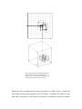
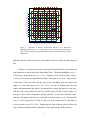
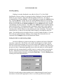
The CMAC design subdivides variable space into a shingled
framework of overlapping blocks whose incremental offsets describes a finer mesh of
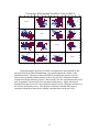
cells. The basic idea is shown in the simplified diagrams for two- and three variablespace in Figure 1, but is easily extended to higher dimensions. Relatively complex
patterns can be stored in this architecture, which results in large savings of computer
memory as compared with a conventional gridded cell division. The contents of the
blocks can be rapidly modified to collectively generate complex associations at much
greater speeds than their equivalent computation through mathematical equations. This
property is important for practical real-time performance in robot applications with
control of elaborate articulated movements.
The implementation of the CMAC design by the robotics community predated the
introduction of neural networks for artificial intelligence applications and has some
design features in common. According to Burgin (1992), a CMAC is most closely
comparable to a feed-forward neural network that is trained by back-propagation, but
almost always outperforms the neural network. So, CMACs can be easily adapted to
function as data analysis tools beyond their original purpose as robot controllers. While
1
Y
X
Z
Y
X
Figure 1: Basic structure of KIPLING/CMAC data storage
architecture with two inputs (above) and three inputs
(below). In each case, responses located within a grid cell
are coded as the overlap of a unique set of blocks.
Kipling.xla does not implement the iterative operation of a CMAC device, it retains the
data storage architecture design that is the core feature. In addition, the ability to store
data either as frequencies of occurrence or properties of continuous or discrete variables
2
allows Kipling to function both as a discrete classifier and a continuous predictor. As
will be discussed in the next section, the overall approach has strong similarities with
ASH (average shifted histogram) procedures. Finally, Kipling was developed at the
Kansas Geological Survey primarily for log analysis applications.
However, the
methodology is highly generalized, so that Kipling can be applied to almost any kind of
data.
From CMAC to ASH
Kipling can be used for either nonparametric regression or nonparametric
discriminant analysis, developing a model for the prediction of either a continuous
variable (such as permeability) or a categorical variable (such as facies) based on a set of
underlying predictor variables (a set of well logs, for example). It can also be run in both
modes simultaneously, developing different regression-type relationships for data from
different categories.
The definition of a nonparametric estimator is open to some debate. In fact, the
term “nonparametric” is a bit of a misnomer, since most nonparametric models are in fact
characterized by a very large number of parameters (data counts in each bin of a
histogram, for example). In contrast, most parametric models are characterized by a
small number of parameters (e.g., the mean and variance of a normal distribution). The
primary practical distinction between parametric and nonparametric estimators is that the
former are generally global, depending on the entire data set at hand, whereas
nonparametric estimators are generally localized in some fashion. Scott (1992) writes,
“If
fˆ (x )
is a nonparametric estimator, the influence of a point should vanish
asymptotically if x − xi > ε for any ε > 0 , while the influence of distant points does not
vansih for a parametric estimator.” A nonparametric estimator provides smoothed or
summary descriptions of the behavior a function in a large number of local
neighborhoods in the space of the independent variables, x, rather than a single global
summary over the entire space.
3
Kipling was originally developed in terms of the Cerebellar Model Arithmetic
Computer (CMAC) algorithm described by Albus (1981). The critical feature of the
CMAC is its means of discretizing the variable space, which results in both memory
savings and in the algorithm's ability to generalize from a set of training data without
reducing the data distribution to a simplified parametric representation. Although Albus
(1981) presents the CMAC discretization scheme using neurobiological terminology, it
really amounts to nothing more than dividing each input (predictor) variable axis into a
set of bins and then determining the location of each data point in terms of its bin number
along each axis. The interesting feature of the CMAC scheme is that more than one such
binning of the variable space is used. Each alternative binning ("layer") employs the
same bin widths, but the bin origin is offset by a fixed amount from one layer to the next.
If l layers are used, then the offset along each axis is 1/l times the bin width along that
axis. The d-dimensional bins in each layer overlap with those in other layers, forming a
set of smaller d-dimensional cells, each defined by a unique combination of bins from the
l different layers. Essentially, the learning phase of CMAC amounts to adjusting the
values (averages of a dependent variable or data counts) associated with each larger bin,
while the prediction phase employs the values associated with each smaller cell, derived
from averaging the contributions of the l different bins defining that cell. This procedure
allows a prediction at the scale of the smaller cells that retains the generalization
(smoothing) associated with the scale of the larger bins.
The CMAC's discretization of variable space is exactly equivalent to the averaged
shifted histogram proposed by Scott (1992). In fact, Scott's algorithm is somewhat more
general, in that the bin offsets from one layer to the next are not constrained to 1/l times
the bin width, but may take on any value. However, the 1/l offset results in a convenient
simplification and does not greatly reduce the effectiveness of the algorithm.
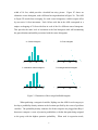
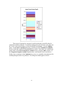
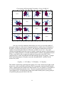
The
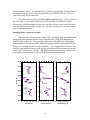
concept of the averaged shifted histogram (ASH) is illustrated in Figure 2. The data
consist of 307 values of the thickness, in feet, of the Morrison formation in northwestern
Kansas. The histogram in Figure 2A uses a bin width of 50 feet, providing a fairly coarse
but stable representation of the data distribution. The histogram in Figure 2B uses a bin
4
width of 10 feet, which provides a detailed but noisy picture. Figure 2C shows an
alternative coarse histogram, with a different bin origin than that in Figure 2A. The ASH
in Figure 2D results from averaging five such coarse histograms, with bin origins offset
by successive 10-foot increments. Each 10-foot wide bin in the ASH corresponds to a
unique overlapping of 50-foot wide bins in each of the five different coarse histograms.
This provides the same level of resolution as the fine histogram while still maintaining
the generalization and stability associated with the coarse histograms.
A. Coarse histogram
0
100
200
B. Fine histogram
300
0
C. Alternative coarse histogram
0
100
200
100
200
300
D. Averaged shifted histogram
300
0
100
200
300
Figure 2. Illustration of the averaged shifted histogram
When predicting a categorical variable, Kipling uses the ASH for each category to
develop a probability density estimate at the location specified by the vector of predictor
variables. The probability density estimates for all the categories are plugged into Bayes'
theorem to compute a vector of posterior probabilities, with the data point being assigned
to the group with the highest posterior probability. When used in regression mode,
5
Kipling also stores the averages of the dependent variable in each bin and bases its
prediction on these bin-wise averages.
This varies only slightly from the CMAC
algorithm, which uses an iterative procedure to adjust the dependent variable values
associated with each bin, attempting to reduce the sum of absolute deviations between
observed and predicted values.
Discretization details
The discretization scheme employed in Kipling is most easily illustrated in one
and two dimensions, although the same scheme applies without modification to higher
dimensions. Figure 3 illustrates the Kipling discretization scheme in one dimension. In
this case, it is desired to represent the behavior of a function over a range of x values
(2,2,1)
(5,4,4)
from –13 to 13, with a fundamental resolution of 2 units at the fine scale of discretization.
combined
1
2
3
4
5
layer 3
1
layer 2
2
1
layer 1
-15
2
-10
4
3
3
-5
4
0
x
5
5
5
10
15
Figure 3. One-dimensional illustration of Kipling discretization scheme.
6
In this case, we have chosen to use three layers of coarse bins, requiring a width of 6
units for each bin. The bin origin for each successive layer is offset from the origin of the
previous layer by 2 units. As shown in Figure 3, each 2-unit interval at the fine scale of
resolution is associated with a unique combination of bins from each of the three layers.
Throughout the following discussion, the coarse-scale intervals will be referred to as
“bins” and the fine-scale intervals will be referred to as “cells”, simply as a convenient
means of distinguishing the two. The terminology is arbitrary. The locations of the cell
centers will be referred to as grid nodes or just nodes. The grid nodes are represented by
the circles in Figure 3, while the plusses mark the cell boundaries.
It is clear from figure 3 that the discretization scheme could be specified in either
of two ways. The user could specify the bin width, wb, and the number of layers, l. This
would result in a bin origin offset of wb/l from one layer to the next, thus determining the
cell width, wc = wb/l. Alternatively, the user could specify the cell width and the number
of layers, resulting in a bin width of wb = l*wc. The latter approach is employed in
Kipling, since it is more convenient in higher dimensions for the user to enter the
specifications of a grid of cells, with a minimum and maximum grid node location and a
cell width (grid increment) being given for each axis. The bin width along each axis is
then given by the number of layers times the cell width along that axis.
The Kipling training process consists of identifying the set of bins containing each
training data point, incrementing the data count for each of those bins, and, for
regression-type applications, updating the bin-wise averages of the dependent variable
according to the dependent variable value associated with the data point. In prediction
phase, each prediction data point is similarly located in terms of a corresponding set of
bins. The predicted density estimate for that location is computed by combining the data
counts for all the bins, while the predicted dependent variable is computed from
combining the bin-wise averages. All data points associated with the same set of bins
(that is, falling within the same cell) are essentially indistinguishable and will be
associated with the same predicted values.
7
Determining the set of bins associated with a given data point, x, is accomplished
by first determining the index of the cell containing x and then mapping that cell index to
the appropriate set of bin indices. The cell index is given by
i = int (( x − x min + 0.5dx ) dx ) + 1
where xmin is the location of the first grid node (cell center) and dx is the cell width (wc
above). For the example shown in Figure 3, with xmin = -12 and dx = 2, every point in the
range 7 ≤ x < 9 will be mapped to a cell index of i = 11 (or, in other words, to node 11, at
x = 8). If there are l layers of bins, then the cell index is mapped to the bin index, k, in
layer j, using:
ì int (i l ) + 1 if
k=í
îint (i l ) + 2 if
j ≥ mod(i, l )
j < mod(i, l )
where mod(i,l) represents the integer remainder from the division of i by l. Since
int(11/3) = 3 and mod(11,3) = 2, cell 11 in Figure 3 corresponds to bin 5 in layer 1, bin 4
in layer 2, and bin 4 in layer 3, or to the unique combination (5,4,4), as shown. In d
dimensions, this formula is applied along each axis to locate the set of d-dimensional bins
containing the data vector x.
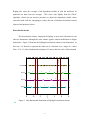
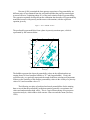
Figure 4 illustrates the Kipling discretization scheme in two dimensions. In this
example we have added a second variable, y, to the one-dimensional example above and
have discretized y into grid nodes ranging in value from 15 to 75 with an increment of 5,
retaining the same discretization (-12 to 12 by 2) for the x variable. This yields the same
number of grid nodes (13) in each direction, which is convenient for illustration but is in
no way required by the software. Employing three layers of bins, as before, yields bin
widths of 6 units in the x direction and 15 units in the y direction. In general, the
variables employed in an analysis may be incommensurate, so that grid increments and
bin widths would vary significantly from one axis to the next. However, the number of
8
75
70
65
60
55
y
50
45
40
35
30
25
20
15
-12-10 -8 -6 -4 -2 0 2 4 6 8 10 12
x
Figure 4. Illustration of Kipling discretization scheme in two dimensions.
Highlighted grid node at (x,y) = (8,45) maps to bin (5,3) in the first layer (solid lines),
bin (4,3) in the second layer (long-dashed lines), and bin (4,3)in the third layer (shortdashed lines).
grid nodes per bin (which is the same as the number of layers) will be the same along all
axes.
In Figure 4, the first layer of bins is represented using solid lines, the second with
long-dashed lines, and the third with short-dashed lines. The node highlighted, at (x,y) =
(8,45) maps to node indices of (ix,iy) = (11,7). Along the x axis, this node maps to bins 5,
4, and 4, just as in the one-dimensional example. Along the y axis, node 7 maps to bin 3
in each layer. Thus, the node, and any point in the surrounding grid cell, maps to the
unique set of bin index pairs [(5,3), (4,3), (4,3)]. In fact, the Kipling code does not
employ multidimensional bin indices, but instead uses a single bin index for each layer,
with the index cycling fastest over the first variable, then over the second variable, etc.
In Figure 4 this would correspond to starting with bin 1 in the lower left-hand corner,
with bins 1 through 5 in the first row, 6 through 10 in the second row, etc. Thus the node
at (x,y) = (8,45) maps to bin 15 in the first layer, 14 in the second, and 14 in the third, or
to the bin index vector (15,14,14). Employing the single indexing scheme allows the
code to function without alteration regardless of the dimensionality of the problem.
9
In higher dimensions, the use of a set of overlapping large bins results in
considerable savings in required storage space relative to using the fine grid directly. The
number of grid nodes in Figure 4 is 132 = 169. The number of bins, however, is 75 (25
bins per layer). If there are l layers and c nodes along a given axis, then the number of
bins along that axis is given by
ì int ((c − 1) l ) + 1 if
m=í
îint ((c − 1) l ) + 2 if
mod(c − 1, l ) = 0
mod(c − 1, l ) ≠ 0
The first case occurs when the number of nodes minus one is evenly divisible by the
number of layers.
Otherwise, we must add one “extra” bin along the axis to
accommodate the remaining nodes.
For example, for a 5-dimensional problem
employing 20 grid nodes along each axis, the total number of grid nodes is 205 =
3,200,000. Using 7 layers of bins results in 4 bins per layer along each axis, or 45 = 1024
bins per layer, for a total of 7168 bins. The use of the overlapping bins also results in the
algorithm’s ability to generalize from sparse data, since the influence of each data point is
spread out over the region encompassed by all the bins in which it falls. In fact, the
process of building an ASH can be viewed as a primitive kernel estimation process, with
the kernel function appearing as a stepped isosceles triangle (in one dimension),
representing the number of bins overlapping a data point as a function of distance from
the grid cell containing the data point. Scott (1992) provides a detailed discussion of the
connections between ASH estimators and those based on continuous kernel functions.
This generalization process is very important for higher-dimensional problems.
As the number of dimensions increases, it becomes increasingly likely that any given
region of variable space will be empty, even for fairly uniformly distributed data (Scott,
1992). Thus it is important to spread the influence of each data point over a fairly large
region of variable space during the training phase of Kipling in order to avoid having a
large number of data points falling in “empty space” during the prediction phase. The
relative emptiness of high-dimensional space also results in a great reduction in the
10
amount of information that needs to be retained from the training phase, since the vast
majority of bins will in fact be empty. Only the layer number, bin index, data count, and
(optionally) average response variable for each non-empty bin need be retained for each
category employed in the analysis. This collection of information is rather loosely
referred to as a “histogram” in the Kipling code. In most applications the number of nonempty bins will be a small fraction of the total number of bins.
Predicting a continuous variable
For regression-type applications, the training phase of Kipling consists of
computing the average value of the dependent variable over each bin. The data count for
each bin is also retained.
The result of the training process consists of a single
“histogram” containing the layer number, bin index, data count, and average dependent
variable for each non-empty bin. During the prediction phase, each prediction data point
is first located in the proper grid cell in the predictor variable space and that cell is
mapped to the appropriate set of bins. The predicted response variable for the data point
is computed as the average of the bin-wise averages for the non-empty bins. If all of the
bins associated with a prediction point are empty, then no response value will be
computed for that point. The associated density estimate (derived from the data count, as
discussed below) will be zero, indicating that an appropriate value for the response
variable is in fact unknown, due to lack of training data in this region of space.
Predicting a categorical variable
If the user supplies a categorical response variable during the training phase, then
a different histogram is returned for each of the different categories. (The categorical
variable should consist of a set of integers ranging from 1 to the number of categories.
Values outside this range are considered unknown and the corresponding data points are
ignored during training.)
The data counts for each category in each layer of bins
constitutes an alternative coarse histogram for that category. The data count for category
i in bin k can be converted into a probability density estimate for that category using
11
f i ,k =
ni , k
ni v b
where ni,k is the number of data in category i in bin k, ni is the total number of data in
category i, and vb is the bin volume (the product of the bin widths along all axes). During
the prediction phase, each prediction data point is first mapped to the appropriate grid cell
and then the probability density estimate for that cell is obtained by averaging the density
estimates for the set of bins (one from each layer) constituting that cell. These cell-wise
density estimates for category i define a probability density function, f i (x ) , which varies
over the space of predictor variables, x.
If there are g different categories or groups, each occurring with “prior”
probability qi, Bayes’ theorem gives the posterior probability of occurrence of group i
given the observed vector, x, as
p(i | x ) =
qi f i (x )
g
å q j f j (x )
j =1
The prior probabilities represent the investigator’s estimate of the overall prevalence of
each group, in the absence of information on the predictor variables. The posterior
probability reflects the probability that an observation has arisen from group i
conditioned on the fact that a particular vector x has been observed. If the density
estimate for one group in the neighborhood of x is much higher than that for another
group, then it is more likely that the observation has arisen from the first group,
regardless of the prior probabilities. The predicted category for each data point is that
associated with the highest posterior probability.
12
Kipling gives the user three options for specifying the prior probabilities, qi. The
first two are those offered by most standard statistical packages, representing either equal
priors for all groups:
q i = 1 g , i = 1, K , g
or prior probabilities proportional to the number of data in each category in the training
data set:
q i = ni n
where n is the total number of training data. The third option for computing prior
probabilities is unique to Kipling and yields values for qi that actually vary over the
predictor space. In this case the value of qi associated with each grid cell is determined
by the number of non-empty bins for category i at that point. If hi of the bins associated
with a grid cell contain data points from category i, then qi is given by
qi =
hi
g
åhj
j =1
For example, assume that there are two categories and that five layers of bins are being
employed. If three of the bins associated with a cell contain data points from the first
group and four of the bins contain data points from the second group, then the prior
probabilities for the two groups at that cell would be by 3/7 and 4/7 respectively. These
“adaptive” prior probabilities vary over the space of predictor variables, unlike the
traditional global prior probabilities, but are less sensitive to the local details of the data
distribution than the density estimates, f i (x ) . The density estimates depend on the data
counts in each bin while the adaptive priors depend only on the presence or absence of
data.
13
Simultaneous prediction of continuous and categorical variables
Kipling allows the user to specify both a continuous response variable and a
categorical response variable. During the training phase a “histogram” is developed for
each category, just as in the case in which a categorical variable alone is being employed.
In addition, bin-wise averages of the response variable are also computed, with only the
response variable values for data points from group i contributing to the averages for that
group. During the prediction phase, Kipling produces the set of posterior probabilities
for each prediction data point along with the predicted response variable for each
category, derived from the bin-wise averages for that category. Kipling also returns the
predicted response for the most likely class at each data point and a probability weighted
predicted response given by
g
γˆ w = å pi γˆi
j =1
where pi is the posterior probability for group i and γˆi is the predicted response for group
i.
Incorporating transition probabilities
In many geological applications, the sequence of categories may be meaningful.
For example, the categorical variable may represent facies, in which case one would
expect to see transitions between facies representing physically adjacent depositional
environments more often than transitions between more widely separated environments.
The relative number of transitions between each possible pair of categories can be used to
compute a transition probability matrix, such as that employed in Markov analysis of
facies sequences (Doveton, 1994).
Kipling contains code to compute a transition
probability matrix from an observed sequence of categorical values.
For such
applications Kipling considers the first element in the vector of categorical values to be
14
the “top” and the last element to be the “bottom”. Transitions are counted from the
bottom up, which is appropriate for applications to facies sequences but may be less
appropriate for other applications. The number of transitions from one category to
another are stored in a tally matrix in which the i,jth element, ni,j, represents the number of
times category j occurs above category i.
This matrix is turned into a transition
probability matrix (TPM) by dividing each row by its sum, representing the total number
of transitions upward from category i. That is, based on the observed sequence of
categories, the probability of a transition to category j from category i is given by
ni , j
t i, j =
g
å ni , m
m =1
In a typical application in well log analysis, the data are sampled at regular intervals such
as 1 foot or ½ foot. In this case, long sequences of values may fall in the same category
(facies), implying that the TPM will have values close to 1 on the diagonal and much
smaller values off the diagonal. That is, the next interval up will almost always be in the
same category as the current interval. In many applications, such as Markov chain
analysis, such a TPM would not be used directly, but would instead be modified to reflect
the actual number of transitions from one category to a different category (Doveton,
1994). However, the raw transition probabilities shown above are quite appropriate for
Kipling, which employs the TPM to modify the posterior probabilities of group
membership computed from predictor variables (e.g., logs). The large diagonal elements
in the TPM serve to smooth the sequence of predicted categories, endowing the predicted
sequence with transition frequencies similar to those in the training data set.
The TPM can be used to modify a sequence of membership probability vectors in
the following fashion: If p i0 represents the probability of membership in group i for the
bottom-most interval (interval 0) based on the observed predictor variables, as described
above, then the probability of occurrence of group j for the next interval up (interval 1),
based solely on the transition probabilities, is
15
u 1j =
g
å t k , j p k0
k =1
(Actually, the u values would have to be divided by their sum to be legitimate
probabilities, but they are not employed directly, anyway.)
These transition-based
probabilities are combined with the original probabilities of group membership for
interval 1 to create the modified membership probabilities for interval 1:
w1i
=
u 1i p1i
å u1j p1j
j
The modified probabilities for interval 2 are computed in the same fashion, employing
the modified set of probabilities for interval 1. In general, the modified probabilities for
interval m are given by
wim =
pim å t k ,i wkm−1
å
j
k
m
pj
å t k , j wkm−1
k
with wk0 = p k0 .
16
References
Albus, J.S., 1975, A new approach to manipulator control: The Cerebellar Model
Articulation Controller (CMAC): Transactions of the ASME, September, p. 220-227.
Albus, J. S., 1981, Brains, Behavior, and Robotics, BYTE Publications, Inc.,
Peterborough, N. H., 352 pp.
Burgin, G., 1992, Using cerebellar arithmetic computers: AI Expert, June, p. 32-41.
Doveton, J. H., 1994, Geologic Log Analysis Using Computer Methods, AAPG
Computer Applications in Geology, No. 2, AAPG, Tulsa, OK, 169 pp.
Scott, D. W., 1992, Multivariate Density Estimation:
Visualization, John Wiley & Sons, Inc., New York, 317 pp.
17
Theory, Practice, and
18
RUNNING KIPLING
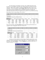
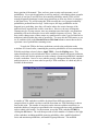
Installing Kipling
Kipling is currently distributed as an add-in for Excel 97 or Excel 2000.
Installing the software consists of copying the add-in, Kipling.xla, from the distribution
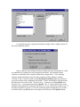
diskette to your computer’s hard drive and then loading it into Excel. The latter is
accomplished by selecting Add-Ins… from the Tools menu to launch the Add-Ins dialog
box. Click the Browse… button and use the resulting Browse dialog box to locate the
add-in file (Kipling.xla). Double-click on the file name or select the name and click OK.
Kipling will be added to the Add-Ins available list on the Add-Ins dialog box, with the
corresponding check box checked. Click OK on the Add-Ins dialog box and the Kipling
add-in will be loaded. The Kipling toolbar (containing a single menu) will be added to
the set of toolbars at the top of the Excel window. You may later unload the add-in by
returning to the Add-Ins dialog box and unchecking the entry for Kipling. The entry will
remain in the list, so that you can reload the add-in simply by checking the check box
again. (You should not move the add-in file once you have loaded the add-in. If you do,
Excel will get confused and start whining.) The example files discussed below are
contained in the Examples folder on the distribution diskette.
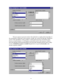
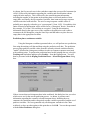
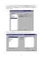
Setting the label row and starting column
In order for Kipling to operate on the data in a worksheet, the layout of that data
must obey certain rules. Specifically, each variable should appear in a single column
while the variable measurements for a given observation should appear in a single row.
The code assumes that variable labels appear in a certain row, with data values starting in
the next row down. Information appearing in rows above the label row will be ignored.
Similarly, the code assumes that the variables begin in a certain column, not necessarily
the first. Information to the left of this column is ignored. You may specify both the
label row and the starting column by selecting Set Label Row… from the Kipling menu,
resulting in the following dialog box:
The label row and starting column numbers may be changed using the arrow boxes to
increment or decrement the appropriate values, or you may type the desired number
19
directly into the edit box. The default values for label row and starting column (4 and 4)
are approriate for use with worksheets generated by the PfEFFER software. However,
other values may also be employed.
The information specified in the Set working range dialog box, above, is used by
the code when it is generating dialog boxes for the selection of variables to analyze.
Occasionally, problems might arise that will cause the software to lose track of the label
row and starting column values. In this case, you will be prompted to reset these values
prior to running an analysis.
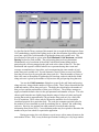
Learning phase, continuous variable
The prediction of a continuous variable will be illustrated using core permeability
and logging measurements from the Lower Permian Chase group in the Hugoton gas
field in southwest Kansas. This represents a regression-style application, with logging
measurements of the porosity and the uranium component of the spectral gamma ray log
being used to explain or predict core permeabilities. The training phase will employ logs
and core permeabilities from one well, and then prediction will be performed in a nearby
well in which only logs are available. The depth variation of the porosity, uranium, and
permeability over the section of interest in the training well are as follows:
2700
2725
2750
Depth (ft)
2775
2800
2825
2850
2875
2900
0
5
10
15
20
Porosity (%)
25
0
1
2
3
4
5
Uranium (ppm)
20
6
0.01 0.10 1.00 10.00
Permeability (md)
Doveton (1994) examined the least squares regressions of log-permeability on
different pairs of logs obtained from the well and found that the porosity-uranium pair
was most effective, explaining about 41% of the total variation in the log-permeability.
The regression equation developed from the calibration data describes a log-permeability
trend that increases with porosity and decreases with uranium, with the regression
equation given by
log K = −0.13 + 0.09 Φ − 0.22 U
The predicted log-permeabilities form a plane in porosity-uranium space, which is
represented by the contours below:
0.1
m
d
6
5
d
1m
3
10
md
Uranium
4
2
1
0
0
4
8
12
Porosity (%)
16
20
The bubbles represent the observed permeability values in the calibration data set,
ranging from 0.014 md (smallest bubble) to 32.7 md (largest bubble). Clearly the
regression only very generally represents the trends in the data, missing such important
features as the clustering of the smallest permeability values in the vicinity of a porosity
value of 4% and a uranium value of 2.
The following two plots of predicted and actual permeabilities for the training
data set reveal that the permeability prediction equation generally overestimates low
values and underestimates high values. This is a typical shortcoming of least-squares
regression analysis, which tends to shift extreme values towards the mean (Doveton,
1994).
21
1.00
0.10
0.01
0.01
0.10
1.00
10.00
Observed Permeability (md)
2875
Observed
Predicted
2900
2925
Depth (ft)
Predicted Permeability (md)
10.00
2950
2975
3000
3025
0.01 0.10 1.00 10.00
Permeability (md)
22
We will attempt to use Kipling to develop a more faithful description of the
dependence of permeability on porosity and uranium than that provided by the linear
regression. Data for this example are contained in Chase.xls, which consists of two
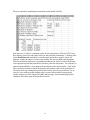
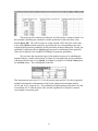
worksheets. The first worksheet, labeled Training well, contains the depth, porosity,
matrix apparent density and photoelectric absorption, the thorium, uranium, and
potassium components of the spectral gamma ray log, and the core permeability and logpermeability values for the training well, as follows:
The second worksheet, labeled Prediction well, contains the log measurements over
roughly the same stratigraphic interval in a nearby well:
As shown, the first variable on both worksheets (Depth) appears in the second
column (B) and the variable labels appear in the fifth row. To prepare Kipling to read
these data, select Set Label Row… from the Kipling menu, and set the label row to 5
and start column to 2, as follows:
23
Having told Kipling that the variable labels reside in row 5 and the first variable is in
column 2, we are ready to proceed with the learning phase, using the training data set.
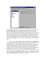
With the Training well worksheet selected, choose Learn… from the Kipling
menu. You will then be presented with the Kipling Training Phase – Select Variables
dialog box:
The list of variables in the worksheet is displayed in the list box in the upper left. The
Add button may be used to transfer any of these variables to the Selected Predictor
Variables list box. Variables in this list box will be the independent variables in the
analysis, those used to explain or predict the chosen continuous and/or categorical
response variables. For this example, we want to transfer the variables Phi (%) and U
(ppm) to the Selected Predictor Variables list box. You can accomplish this by
highlighting each variable in turn (with a single click on the entry in the Variables in
worksheet list box) and clicking the Add button or by selecting both variables (by
clicking on the first and then ctrl-clicking on the second) and then clicking the Add
button. (Contiguous selections may be made by dragging over the desired variables or
clicking on the first variable and then shift-clicking on the last.) After transferring these
variables, the dialog box should appear as follows:
24
The least-squares regression analysis described above employed the logarithm of
the permeability (LogPerm) as the response variable, due to the fact that this variable has
a more linear dependence on the predictor variables than does the permeability itself.
However, in this analysis we will employ permeability itself as the response variable,
since the Kipling prediction methodology can represent nonlinear behavior more readily.
Use the Continuous response variable dropdown list to specify Perm (md) as the
desired response variable:
25
The kind of analysis performed (continuous or categorical) will depend on which kind of
response variable is selected. Selecting both a continuous and a categorical response
variable will result in a simultaneous analysis, with a different regression-type
relationship between the continuous response variable and the predictor variables being
developed for each different value of the selected categorical variable. In this case we
have no categorical variable to employ and so will continue with only a continuous
response variable specified.
The Comment text box allows you to enter a comment that will be recorded in
the first cell of the “histogram” worksheet that will be the product of the training phase.
In this case, you could enter a comment like “Training for prediction of Perm (md)”:
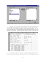
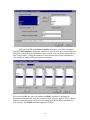
After clicking OK on the Select Variables dialog box, you will be presented with
the Kipling Training Phase – Grid Parameters dialog box:
26
As described in the Theory portion of this manual, the averaged shifted histogram (Scott,
1992) methodology employed in Kipling involves the discretization of predictor variable
space into a grid with a certain number of grid nodes along each variable axis. The
specifications of this grid are given in the Grid Minimum, Grid Maximum, and Grid
Spacing list box for each variable. The grid spacing along each axis determines
fundamental level of resolution of the model, with all data points falling inside a
particular grid cell being mapped to the grid node at the center of that cell. The data
distribution and response variable behavior are represented using data counts and
averages accumulated over larger bins, each encompassing the same number of grid
nodes along each variable axis. Several alternative layers of bins are used, each offset
from the previous layer by one grid node along each axis. Thus the number of layers of
bins is the same as the number of grid nodes per bin along each axis and the bin width
along each axis is given by the number of layers times the grid spacing along that axis.
You use the Grid Parameters dialog box to specify the grid limits and spacing
along each axis, along with the number of layers of bins. These values determine the bin
width and number of bins along each axis. The dialog box also displays the number of
bins per layer and the total number of bins (over all layers). The software attempts to
supply reasonable default values for the grid parameters and number of layers. The code
chooses grid limits that are slightly larger than the range of observed values and a grid
spacing that results in approximately 100 grid nodes along each axis, for a fairly fine
level of resolution. These values may be adjusted to match the level of resolution
considered practical for a particular study. The code also computes an initial value for
the number of layers intended to result in something like an “optimal” bin width along
each axis. However, the optimal bin width estimate is based on rather sketchy
information from Scott (1992). Crossvalidation studies may be required to determine the
number of layers best suited for a particular application.
During processing, the code allocates several arrays with as many elements as the
total number of bins. Thus, it may be that specifications resulting in a very large number
27
of bins will exceed the memory capacity of the computer, requiring you to change
specifications to reduce the number of bins. However, only the values for the non-empty
bins will be written to the histogram worksheet. As described in the theory portion of the
manual, as the number of variables increases, so does the proportion of empty bins, with
almost all of variable space being empty for higher-dimensional problems. Thus, as long
as your computer has enough memory to handle the temporary allocation of a few large
arrays, there is no reason to be timid about specifying a discretization resulting in a very
large number of bins. It is quite likely that information for only a small proportion of the
bins (the non-empty ones) will be written to the histogram worksheet.
For this example we will basically “clean up” the grid limits and increments
supplied by the code, leaving the number of layers at the initial value of 10. First we will
change the grid specifications for the porosity. Highlight the row of values associated
with Phi (%) by clicking ONCE on any entry in that row in the set of list boxes. Then
click the Edit… button to reveal the Edit Grid Parameters dialog box:
Edit the entries in the text boxes to specify a grid of porosity values ranging from 0 to
20% in increments of 0.2%, as shown above. Note that the range of observed values is
shown on the dialog box to provide some guidance in selecting appropriate grid limits. In
the same fashion, change the specifications for uranium so that the grid runs from 0 to 6
ppm in increments of 0.06 ppm. With 10 layers of bins, this results in bin widths of 2%
along the porosity axis and 0.6 ppm along the uranium axis, with 11X11 =121 bins per
layer, for a total of 1210 bins, as shown below:
28
After setting the desired grid parameters, click the OK button. The code will then
process the training data, writing the relevant results to a “histogram” worksheet. Each
histogram worksheet is given a name like Hist01 or Hist02, with the number
corresponding to the order in which it was created. You should not alter either the name
or the contents of a histogram worksheet. If you do, the code implementing the
prediction phase will not be able to locate or employ the histogram information.
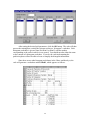
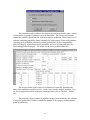
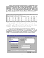
Since there are no other histogram worksheets in the Chase workbook yet, the
code will generate a worksheet entitled Hist01, which appears as follows:
29
As shown, the first several rows in the worksheet contain the user-specified comment (in
cell A1) followed by information regarding the variables and discretization scheme
employed in the analysis. This is followed by the actual histogram information,
including the number of data points in the training data set, the total number of nonempty bins, and, finally, the layer number, bin index, data count and average response
variable associated with each bin. The set of average response variable values is
probably more properly referred to as a “regressogram” (Scott, 1992). Nevertheless, this
entire collection of information will be referred to as a “histogram” herein. Note that in
this example, 541 of the 1210 total bins are occupied. Using the discretization
information listed in the upper rows of the worksheet, the prediction code is able to
reconstruct the full histogram, using the listed layer and bin indices to place the nonempty bins in the appropriate locations.
Prediction phase, continuous variable
Using the histogram worksheet generated above, we will perform two predictions,
first using the training well data and then using the prediction well data. The prediction
process plugs predictor variable values from the currently selected worksheet into the
“model” described in a histogram worksheet in order to compute responses associated
with each data point. To perform the prediction based on the training data set, select the
Training well worksheet and then select Predict… from the Kipling menu. You will
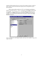
then be presented with the Kipling Prediction Phase – Select Histogram Sheet dialog
box:
If there is more than one histogram sheet in the workbook, this dialog box lets you select
which one to use for the current prediction process. As shown, it presents some
information regarding the currently selected histogram sheet, including the user
comment, the continuous and/or categorical response variable represented, and the set of
predictor variables. We have generated only one histogram worksheet in the Chase
workbook, so have no other option at this point but to click OK. You are then presented
with the Select Predictors dialog box:
30
This dialog box is asking you to specify which of the variables in the current worksheet
(in the Available Logs list box) correspond with the predictor variables used in the
production of the histogram worksheet (represented by the names on the buttons).
Because we are using the same worksheet that we used in the training process, we happen
to have variables whose names (Phi (%) and U (ppm)) correspond exactly with those
used in the training process. However, it is quite possible that variable names will differ
between worksheets, leading to the need for this dialog box. In this case, first select
(with a single click) Phi (%) in the list box and then click the Phi%>> button to transfer
that variable to the Chosen text box. Then do the same for U (ppm) and click the OK
button.
You will then be presented with the Select Variables to Copy to Output dialog
box, shown on the next page. This dialog box allows you to choose a set of variables that
you would like to have copied from the current worksheet to the new worksheet
containing prediction results. For example, in log analysis applications it will usually be
helpful to copy the depth column to the new worksheet, to allow plotting of predicted
results versus depth. Also, if you have observed values of the predicted variable
available you may also want to copy these to the new sheet, for ease of comparison with
the predicted values. In this case we will copy both the depth and the observed
permeability values to the new worksheet. Transfer the desired variables by selecting the
appropriate entries in the Variables in worksheet list box and clicking Add>> to transfer
them to the Selected Variables to Copy list box. After transferring Depth (ft) and Perm
(md) to the right-hand list box, as shown below, click OK.
31
The software now proceeds to compute the predicted permeabilities based on the
values of the predictor variables in the current worksheet, writing the results to a new
worksheet. The new worksheet will be given a generic name such as Sheet5. You are
free to change this name to a more meaningful one by double-clicking on the sheet’s tab
and typing in a new name. The prediction results worksheet we just created looks like:
The initial lines of information essentially describe the genesis of the prediction
results contained in the worksheet. These lines are followed by the prediction results
themselves, with the variables copied from the prediction data set occupying the first few
32
columns. For continuous-variable prediction, the columns containing copied variables
are followed by two columns, one labeled Density and the other labeled Predicted var,
where var is replaced by the actual name of the variable being predicted, as specified in
the histogram worksheet. The Density column contains the probability density estimate
associated with each prediction data point, based on the distribution of the predictor
variables in the training data set (that used to produce the histogram). The Predicted var
column contains the estimated response variable associated with each prediction data
point, based on the bin-wise average response values contained in the histogram
worksheet. If the probability density estimate for a given point is zero, meaning that the
prediction data point falls in a region of space containing no training data, then the
corresponding cell in the Predicted var column will be empty, due to the lack of
information from which to compute a response variable value. When a categorical
variable is included in the analysis, additional columns will appear on the worksheet.
These will be described in the section on categorical variable prediction.
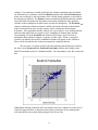
We can create a crossplot of observed and predicted permeabitilies by selecting
the values in the Perm (md) and Predicted Perm (md) columns and clicking on the
Chart Wizard button on Excel’s Standard toolbar. On a logarithmic scale, the results look
like:
Although the Kipling predictions still overestimate some low conductivity values, this is
clearly an improvement over the linear least-squares predictions for the training data,
with considerably more points falling along the one-to-one line.
33
We will next use the “model” represented in the Hist01 worksheet to compute
permeability in the prediction well. Switch to the Prediction well worksheet and then
select Predict… from the Kipling menu. Once again select Phi (%) and U (ppm) as the
predictor variables
and then select Depth (ft) as the variable to copy to the output worksheet:
34
The new worksheet containing the prediction results should look like:
Note that rows 13 and 14, containing results for the predictions at 2700 and 2700.5 feet,
have density values of 0 and empty values for the predicted permeability. Checking back
on the Prediction well worksheet reveals that these points have negative values for
uranium, outside the range of values in the training data and encoded in the histogram.
Thus the prediction results quite reasonably demonstrate the model’s lack of knowledge
of an appropriate predicted permeability for these particular data points. The sequence of
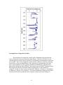
predicted permeabilities versus depth in the prediction well is shown below. Gaps in the
curve represent locations at which the porosity and uranium values in the training well
fall too far from any training data point for the model to provide any prediction. As an
exercise, you could repeat the training using a coarser discretization (increasing the
number of layers to create larger bin widths and/or using a coarser underlying grid) to
attempt to fill in these gaps in the prediction results.
35
Learning Phase, Categorical Variable
The prediction of a categorical variable will be illustrated using logs from the
Lower Cretaceous in two wells in north central Kansas. The first well, Jones #1, was
cored through the section of interest and facies assignments based on analysis of this core
are available. These facies designations will be used to calibrate a model for predicting
facies from six logs, including thorium (TH), uranium (U), and potassium (K) values
from a spectral gamma ray log, apparent grain density (RHOMAA), apparent matrix
photoelectric absorption factor (UMAA), and neutron porosity (PHIN). Kipling requires
that categorical values be specified as integers ranging from 1 to the number of
categories. In this case the six facies are encoded 1 (Marine), 2 (Paralic), 3 (Floodplain),
4 (Channel), 5 (Splay), and 6 (Paleosol). The model obtained from training on the Jones
well data will be used to predict the facies sequence in the second well, Kenyon #1.
36
The data from the Jones well is contained in the Jones.xls workbook. This
happens to be a PfEFFER workbook, with the first variable (Depth) in column four and
variable labels appearing in row 4. Thus, Kipling’s default values of 4 and 4 for the label
row and starting column are appropriate in this case. Select Set Label Row… from the
Kipling menu to verify or set these values, as needed.
The relevant data in Jones.xls appear in columns Q through X of the Lower
Cretaceous worksheet:
The sequence of core-assigned facies values versus depth appear as follows:
37
The process of training for categorical variable prediction is much like that for
continuous variable prediction. To start the training process for the Jones well, make sure
the Lower Cretaceous worksheet is selected and then select Learn… from the Kipling
menu. On the Select Variables dialog box, scroll down in the Variables in worksheet
list box so that the variables TH through PHIN are visible. Select these six variables and
transfer them to the Selected Predictor Variables list box using the Add>> button. In
the Categorical response variable dropdown box, scroll down to facies and select it.
Finally, enter a comment in the Comment box to serve as a reminder concerning how the
resulting histogram sheet was produced. The dialog box should appear as below:
38
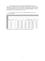
After you click OK on the Select Variables dialog box, you will be presented
with the Grid Parameters dialog box. In this case we will use a much coarser grid than
that given by the default grid parameter values, with 24 to 28 grid nodes along each axis
and 7 layers of bins. Change the number of layers and edit the grid specifications for
each variable so that the dialog box appears as follows:
After you click OK, the code will produce the Hist01 worksheet, containing the
histogram information (bin-wise data counts) for each of the six separate facies. During
prediction, these bin counts will be used to compute probability density estimates for
each category. The Hist01 worksheet appears as follows:
39
Prediction Phase, Categorical Variable:
Before attempting to predict facies in the Kenyon #1 well, we will first apply the
above facies information to the Jones well data, in order to compare predicted facies to
the facies assignments from core. To do this, switch back to the Lower Cretaceous
worksheet and select Predict… from the Kipling menu. Click OK on the Select
Histogram Sheet dialog box, since Hist01 is the only histogram sheet available. Use the
Select Predictors dialog box to establish the correspondence between predictor variables
on the current worksheet and those used to produce the histogram:
40
and then specify that Depth and facies should be transferred from the current worksheet
to the prediction results worksheet:
You are then presented with the Prior Probability Option dialog box. This
allows you to select between the three options for computation of the prior probabilities
to be employed in computing the probabilities of group membership, as described in the
theory portion of the manual. In this case, select the Adaptive option, which computes
prior probabilities based on the number of non-empty bins per category in the vicinity of
each data point:
41
The prediction results worksheet for categorical prediction includes quite a variety
of information, in groups of columns across the worksheet. The first several columns
contain the variables copied from the worksheet used for prediction. Then comes a set of
columns containing probability density estimates for each category, followed by columns
containing prior probability estimates, posterior probabilities of group membership,
predicted category, maximum posterior probability, and a set of group indicators also
representing predicted category. The results for the Jones prediction look like:
The category labels used in each set of columns are created by appending the
name of the categorical variable (“facies”, in this case) with the category numbers. You
are free to replace these labels with more meaningful ones (such as “Marine”, “Paralic”,
etc.).
The predicted category column is populated using a formula linked to the columns
of posterior probabilities, so that it contains the number of the category with the highest
posterior probability:
42
The Max. Probability column simply contains the corresponding maximum probability
value, giving some measure of the degree of certainty in the categorical prediction. An
alternative representation of the predicted category is contained in the Group Indicators
columns, which are also populated using formula links to the columns of posterior
probabilities:
The group indicators are included on the worksheet for the ease of plotting
predicted categories using the Kipling routine for plotting probabilities, which we will
now employ to examine our results. We will first plot the sequence of posterior
probabilities of group membership versus depth. Before we do so, however, edit column
labels for the posterior probabilities so that they contain the actual facies names:
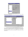
Now select Plot Probabilities… from the Kipling menu to bring up the
Probability or Indicator Plot dialog box:
43
Type a meaningful plot title into the Plot Title edit box and then use the two range
selection boxes to specify the cells containing depth values and those containing the
probability values to be plotted. You can either type the range addresses directly into the
edit boxes or click on the small box at the right end of each edit box to minimize the
dialog box, allowing you to select the appropriate range:
Include the column labels in your selection, as shown. Use the depth values in column A
as the Depth or Time Axis Values and also select Vertically oriented bar chart under
the Plot Format options:
44
After you click OK, Kipling will add the following chart to the worksheet:
45
This plot represents probabilities of membership in all six facies versus depth, based on
the observed log values and the probability density information encoded in the histogram
worksheet. A plot of predicted facies versus depth can be obtained by once again
selecting Plot Probabilities… from the Kipling menu and then selecting the columns of
group indicator values rather than the posterior probabilities. The resulting plot is shown
below, along with the original facies from the core study:
Although there is good overall agreement between observed and predicted facies in this
case, the predicted sequence is quite erratic, with many short segments of facies
interrupting general sequence. This shortcoming can be remedied by incorporating
transition probability information into the predicted probabilities of group membership,
as described later.
In order to use the histogram developed from the Jones well data to predict the
sequence of facies in the Kenyon well, we must first copy the histogram worksheet from
Jones.xls to Kenyon.xls. First open Kenyon.xls, then switch back to Jones.xls, select the
Hist01 worksheet, an then select Move or Copy Sheet… from the Edit menu. On the
Move or Copy dialog box, check the Create a Copy check box and specify that you
want to copy Hist01 to the end of the Kenyon.xls workbook:
46
After copying the worksheet, Excel will automatically switch focus to the new copy of
Hist01 in Kenyon.xls. At this point, switch to the Lower Cretaceous worksheet (in
Kenyon.xls). This worksheet contains values for depth and the six logs in columns Q
through W, but contains no facies values. With the Lower Cretaceous worksheet
selected, choose Predict… from the Kipling menu and repeat the same sequence of
operations used for prediction of facies in the Jones well, except for the copying of the
facies variable, which does not exist on this worksheet. The prediction results worksheet
will look much the same as that in the Jones workbook and plots of posterior probabilities
of facies membership and predicted facies can be produced in the same fashion:
47
These results are even more erratic than those for the Jones well. In the following section
we will attempt to create more reasonable sequences of predicted facies by incorporating
transition probability information computed from the observed sequence in the Jones
well.
Incorporating Transition Probabilities
We will compute a transition probability matrix from the observed sequence of
facies in the Jones well. To do so, select the Lower Cretaceous worksheet in Jones.xls
and then select Compute TPM… from the Kipling menu. On the resulting dialog box
select facies as the categorical variable and then click OK:
The code will then generate a transition probability matrix worksheet named TPM01:
You should not alter the layout of this worksheet. However, you are free to alter the
entries in the transition probability matrix itself. The value contained in row i and
column j of this matrix is the proportion of transitions from category i to category j
relative to the total number of transitions upward from category i, as described in the
48
theory portion of the manual. Thus, each row sums to unity and represents a set of
probabilities. For a typical application in well log analysis, with samples taken at regular
intervals of one foot or one-half foot, the transition probability matrix (TPM) will be
strongly diagonally dominant, because most transitions are from one facies (or category)
to the same facies. We will be using this TPM to modify the set of group membership
probabilities predicted based on logs. In this respect, the large probabilities on the
diagonal are a good thing, since they will tend to reduce the erratic character of the
predicted facies sequence that we have seen above. However, the zero off-diagonal
elements may be of some concern, since any transition associated with a zero transition
probability will not be allowed to occur in the modified sequence of facies. Thus, you
may wish to change some of these entries to a small positive value if you feel that such a
transition is indeed within the realm of possibility. You may edit the TPM entries as you
see fit, and then click on the Rescale Rows to Unit Sum button to ensure that each row
represents a set of probabilities summing to one.
To apply the TPM to the Jones predictions, switch to the prediction results
worksheet we created earlier, containing the posterior probabilities of facies membership.
With this worksheet selected, choose Apply TPM… from the Kipling menu. This
option should only be selected when the active worksheet contains categorical prediction
results, as the code for this option acts on the columns of posterior probabilities contained
in such a worksheet. Just as we were asked to specify a histogram sheet for the original
prediction process, we are now asked to specify a TPM worksheet, of which only one is
available at the moment:
A number of TPM worksheets could be developed from different sequences of
categorical data, in which case there would be more than one TPM worksheet to choose
from at this point. The number of categories on the chosen worksheet would have to
match the number of categories represented in the current prediction results worksheet in
order to obtain valid results. For the moment, accept the TPM worksheet TPM01 by
clicking the OK button. The code then proceeds to add a number of columns to the right
of the worksheet, including modified posterior probability values, modified predicted
facies and maximum probabilities, and modified group indicators. The modified
49
posterior probabilities are computed by combining the original posterior probabilities
(computed from the logs) with the transition probabilities, as described in the theory
portion of the manual. The remaining modified values (group membership, etc.) follow
from the modified posterior probabilities. The modified probabilities and group
indicators can be plotted just as the original values were. The modified sequence of
facies for the Jones well is considerably less erratic and looks much more like the
sequence of assigned facies from core:
In order to apply the TPM to the facies predictions for the Kenyon well, copy the TPM01
worksheet from Jones.xls to Kenyon.xls, just as you did with Hist01, select the prediction
results worksheet in Kenyon.xls, and apply the TPM matrix just as you did for the Jones
well. Plotting the modified probabilities and predicted facies for the Kenyon well reveals
a predicted sequence that is still somewhat erratic, but less so than the predicted sequence
based on the log values alone:
50
Combined Continuous and Categorical Prediction
When both continuous and categorical response variables are specified during the
learning phase, Kipling will generate a histogram worksheet appropriate for combined
categorical and continuous prediction, a process that involves aspects of both
discriminant analysis and regression analysis. Combined prediction will be illustrated
using core logging and grayscale data obtained from two Baltic Sea sediment cores. Both
cores come from the Baltic’s Central Gotland Basin and were obtained during a 1997
cruise of the Research Vessel Petr Kottsov funded under the Baltic Sea System Studies
(BASYS) Subproject 7 (Harff and Winterhalter, 1997). In the Central Gotland Basin, the
upper 4 meters, approximately, of seafloor sediment represents sedimentation since the
opening of the current connection between the Baltic and North Seas about 8000 years
ago. The sediments in this interval alternate between predominately laminated intervals
and more homogeneous intervals. The laminated intervals are taken to represent periods
of prolonged anoxia in the Baltic bottom waters, during which time no benthic fauna
were available to disturb sediment layering. The more homogeneous intervals probably
represent periods during which enhanced exchange between the Baltic and North Seas
provided more oxygenated water to the Baltic Sea floor, allowing populations of benthic
fauna to develop (Harff and Winterhalter, 1997).
51
The two cores employed in this example were obtained with a gravity corer with a
120 mm inner diameter and were taken to the lab at the Baltic Sea Research Institute for
examination. A multisensor core logger (MSCL) was used to measure the p-wave
velocity, wet bulk density, and magnetic susceptibility of the core sediments at 1-cm
intervals and an imaging scanner measured the red, green, and blue components of the
sediment color, at a sampling rate of 12 pixels per millimeter (Endler, 1998). The three
color components are highly correlated and most of the color information is contained in
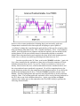
the gray level, which is roughly the average of the three components. The MSCL data for
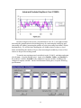
the upper portion of core 211660-5, together with the gray level values smoothed to 1-cm
intervals, are shown below:
MSCL and Grayscale Data, Core 211660-5
Velocity (m/s)
Density (g/cc)
Susceptibility (cgs)
Gray level
0
B6
B5
Depth (cm)
100
B4
200
B3
300
B2
B1
400
1400.00 1420.00 1.00
1.12
1.24
12.00
24.00
80.00
140.00
Core 211660-5 (hereafter abbreviated to 60-5) appears to represent an undisturbed record
of sedimentation for at least the past 8000 years and has been taken as the “master core”
in further analyses. The depth zones labeled B1 through B6 in the figure above were
developed on the basis of depth-constrained cluster analysis (Bohling et al., 1998; Gill et
al., 1993) of the MSCL data together with visual examination and detailed geological
description of the data (Harff et al., 1999a, 1999b). The odd-numbered zones (B1, B3,
B5) roughly correspond with laminated intervals, representing anoxic conditions, while
the even-numbered zones correspond with more homogeneous intervals. The bottom of
the B1 interval (at 378 cm in core 60-5) represents the boundary between Ancylus Lake
and Litorina Sea sediments, a transition corresponding to the opening of the connection
between the Baltic and North Seas.
52
In earlier work, the intervals identified in core 60-5 (the B zones shown above)
were extended into nearby cores in the Gotland Basin by means of correlating the
detrended velocity and density values (Harff et al., 1999a, 1999b; Olea, 1994),
identifying zonal boundaries based on the similarity of the velocity and density curves to
the velocity/density “signature” of the boundary locations in core 60-5. The MSCL and
grayscale data for core 211650-5 (hereafter 50-5), together with the resulting B zone
intervals, look like:
MSCL and Grayscale Data, Core 211650-5
Velocity (m/s)
Density (g/cc)
Susceptibility (cgs)
Gray level
0
B5
100
Depth (cm)
B4
200
B3
B2
B1
300
1400.0 1420.0
1.2
1.4
0.0
10.0
20.0
100.0
200.0
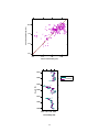
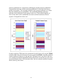
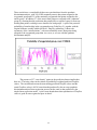
An interesting question to pursue is whether the data values within the identified zones
actually support the segmentation developed from correlating the velocity and density
curves. The crossplots of detrended grayscale and MSCL data for core 60-5 (below)
show the correspondence between the visible and geophysical properties of the core
sediments in this master core, with anoxic/laminated intervals (circles) and
oxygenated/non-laminated intervals (pluses) being reasonably well separated in both
MSCL and grayscale space. It is also apparent that the grayscale values show different
trends with respect to the geophysical variables in the two different kinds of intervals.
53
Crossplots
of
Detrended
Variables, Core
211660-5
-20
-10
0
10
20
-10
-4
2
8
14
60
30
0
GrayRes
-30
-60
20
10
VelRes
0
-10
-20
0.10
0.05
-0.00
DenRes
-0.05
-0.10
14
8
SuscRes
2
-4
-10
-60
-30
0
30
60
-0.10
-0.05
-0.00
0.05
0.10
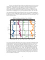
Demonstrating the presence of similar correspondences between MSCL and
grayscale data in the other Gotland Basin cores would support the validity of the
correlation results. The plots of detrended MSCL and grayscale data for core 50-5
(below) show generally similar patterns as those for core 60-5, although with more
overlap between the data from “anoxic” intervals (B1, B3, B5, represented with circles)
and “oxygenated” intervals (B2, B4, represented with pluses). Again, the interval
boundary locations in core 50-5 were transferred from core 60-5 through correlation of
the velocity and density curves. The question of interest is whether the property
variations within these intervals are actually consistent between the two cores.
54
Crossplots
of Detrended
Variables, Core
211650-5
-10
0
10
20
-10
0
10
40
GrayRes
-10
-60
20
10
VelRes
0
-10
0.05
-0.00
DenRes
-0.05
-0.10
10
SuscRes
0
-10
-60
-10
40
-0.10
-0.05
-0.00
0.05
One way to test for consistency between the two cores is to develop models of
grayscale variation or of the anoxic/oxygenated indicator variable (Oxy) as functions of
the MSCL variables in the master core (60-5) and determine whether these models are
capable of reproducing the behavior of the same variables in core 50-5. One could
consider investigating at least three types of models: regression analysis of the detrended
grayscale variable (GrayRes) versus the detrended MSCL variables, discriminant analysis
of Oxy versus MSCL data, or regression analysis of grayscale versus MSCL data
employing Oxy to allow for different trends and intercepts for the two groups. A simple
linear regression analysis of GrayRes versus the detrended MSCL variables for the
master core yields:
GrayRes = -1.34*VelRes + 79.5*DenRes – 2.1*SuscRes
This model is statistically significant and explains 35% of the variation in GrayRes in the
master core, with a correlation coefficient of 0.59 between the actual and fitted GrayRes
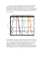
values. Applying the same model to the data from the 50-5 core produces a correlation of
0.44 between actual and predicted values. The plot of predicted and actual GrayRes
versus depth in 50-5 reveals that this simple linear model actually does a pretty good job
of reproducing the grayscale data in this core:
55
Actual and Predicted Grayscale Residual, Core 211650-5
Linear Model
Actual
40
Grayscale Residual
Predicted
20
0
-20
-40
0
50
100
150
200
250
300
Depth (cm)
In terms of the categorical prediction problem, a quadratic discriminant analysis
of the master core data reveals the reasonably good separation of oxygenated and anoxic
intervals in MSCL variable space. Plugging the detrended MSCL data values back into
the resulting discriminant rule produces the following allocation table:
Actual
Anoxic
Oxygenated
Assigned
Oxygenated
49
177
Overall Error Rate
Anoxic
133
20
Error Rate
26.9%
10.2%
18.5%
Applying the same discriminant rule to the detrended MSCL data from core 50-5
results in the following comparison to the “actual” anoxic/oxygenated intervals derived
from the correlation of the velocity and density logs:
Actual
Anoxic
Oxygenated
Assigned
Oxygenated
72
134
Overall Error Rate
Anoxic
104
3
Error Rate
40.9%
2.2%
21.5%
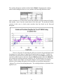
The above allocation results can be represented versus depth in 50-5 by plotting the
probability of membership in the oxygenated group computed from the discriminant rule
56
together with the indicator variable representing the original assignment. The asymmetry
of the allocation results is clear both in the allocation table above and in the plot below:
The discriminant rule assigns almost every data point in the nominally oxygenated
intervals (B2 and B4) to the oxygenated group (probability of membership in oxygenated
group > 0.5) but assigns only 59% of the data points in the nominally anoxic intervals
(B1, B3, B5) to the anoxic group (probability of membership in oxygenated group < 0.5).
This means that many of the observations in zones B1, B3, and B5 in core 50-5 have
detrended MSCL values more like those of the oxygenated (even-numbered) zones in
core 60-5 than the anoxic zones in core 60-5.
Probability of Membership in Oxygenated Group
Probability of Membership in Oxygenated Group in Core 211650-5
Original
1.0
assignment
0.9
Probability
from qda
0.8
0.7
0.6
0.5
0.4
0.3
0.2
0.1
0.0
B5
0
B4
50
100
B3
150
200
B2
250
B1
300
Depth (cm)
A known categorical variable can easily be incorporated as a predictor in a
regression analysis by encoding the n different categories in terms of n-1 indicator values
(with the first category, for example, being represented by zero values for all the indicator
variables and each remaining category represented by a value of 1 for the corresponding
indicator and zero for all others). A linear regression analysis of the grayscale residual
values versus the MSCL residual values in core 60-5, allowing different intercept and
slope estimates for the two different types of intervals, yields the best-fit equation:
GrayRes = (-13.1 + 17.5*Oxy) + (-0.499-0.418*Oxy)*VelRes +
(-21.3+87.7*Oxy)*DenRes + (-0.175-5.850*Oxy)*SuscRes
57
where Oxy = 0 for anoxic intervals and Oxy = 1 for oxygenated intervals. This model
explains 56% of the overall variation in grayscale residual values in core 60-5.
In order to apply this model to prediction of grayscale values in another core, one
would have to supply the indicator value (Oxy) for each location in that core. In the
absence of knowledge of this indicator variable, one could employ discriminant analysis
to predict the probability of membership in the oxygenated group, using the resulting
classification in the above regression equation. One could either use the predicted class
as an indicator variable or, alternatively, employ the probability of membership in the
oxygenated group in place of Oxy in the above equation, resulting in a probabilityweighted mixture of the regression equations for the two classes. We will take the latter
approach for predicting GrayRes in core 50-5, using the probabilities of membership in
the oxygenated group computed from the quadratic discriminant rule in place of Oxy.
Doing so produces a predicted GrayRes whose correlation with the actual GrayRes is
only 0.38, a somewhat worse result than that obtained from the regression model without
Oxy. Compared to the simple linear prediction (without Oxy), the probability-weighted
prediction of GrayRes does a noticeably poorer job of matching the depth variation of the
actual GrayRes in the lower portions of core 50-5:
Actual and Predicted Grayscale Residual, Core 211650-5
Probability-weighted prediction using Oxy
Actual
40
Grayscale Residual
Predicted
20
0
-20
-40
0
50
100
150
Depth (cm)
58
200
250
300
Kipling’s combined categorical/continuous prediction is analogous to the two-step
process of discrminant analysis and regression analysis described above, with the binwise averages of the response variable for training data from each group providing the
nonparametric regression model for that group and the bin-wise data counts for each
group serving as the basis for the nonparametric discriminant analysis. The process will
be illustrated using the data from cores 60-5 and 50-5, contained in the workbook
Baltic.xls. The 211660-5 worksheet contains the data for the master core, as follows:
Because Kipling requires that categorical variables be coded in terms of positive integers,
with 0 representing “unknown”, the Oxy indicator variable in the worksheet is set to 1 for
anoxic intervals and 2 for oxygenated intervals, rather than the more natural 0 and 1
employed above. The worksheet contains both the original variables (Density, Velocity,
Susceptibility, and Gray) and the detrended versions thereof (DenRes, VelRes, SuscRes,
and GrayRes). We will employ the detrended variables in the following.
Prior to training on the master core data, set the label row to 3 and the first
variable column to 1 using the Set Label Row... option on the Kipling menu. Then, with
the 211660-5 worksheet selected, choose Learn… from the Kipling menu. In the Select
Variables dialog box, choose DenRes, VelRes, and SuscRes as the predictor variables,
GrayRes as the continuous response variable, and Oxy as the categorical response
variable:
59
In the Grid Parameters dialog box, change the grid parameters from the default values
to the following more rational values, expanding the grid limits a fair amount from the
default in order to accommodate the range of values in both the master core and in core
50-5, on which we will be predicting:
After you click OK, Kipling will generate the following histogram sheet:
Comparing the contents of this histogram sheet to those for continuous or categorical
prediction alone, it is clear that the combined training process involves nothing more
60
sophisticated than storing the bin-wise averages of the continuous response variable by
group, together with the count information employed for the computation of groupspecific densities.
Before trying to predict results in core 50-5, we will perform a resubstitution
analysis of the data in core 60-5. To do so, switch back to the 211660-5 worksheet and
select Predict… from the Kipling menu. In the Select Histogram Sheet dialog box,
click OK to accept Hist01 as the appropriate histogram worksheet (it is the only one
available so far). Then make the obvious choices of predictor variables in the Select
Predictors dialog box:
In the next dialog box, select Depth, GrayRes, and Oxy as the variables to copy to the
output worksheet:
61
As we did for the pure categorical prediction example, choose adaptive priors for
the prior probability option:
Out to column S, the resulting worksheet contains the same information as would
be contained in a worksheet for pure categorical prediction. The contents of these
columns are explained in the categorical prediction example above. The remaining
columns contain information relevant to the prediction of the continuous variable.
Columns U and V, in this example, contain Predicted GrayRes by Oxy, the predicted
grayscale residual values computed from DenRes, VelRes, and SuscRes using the model
developed for each value of Oxy. Those for Oxy = 1 (anoxic) are labeled fpred1 and
those for Oxy = 2 (oxygenated) are labeled fpred2. The “f” in these labels refers to the
standard representation of a continuous function of a vector of predictor variables, f(x). If
the density estimate for group i is zero and a particular point, meaning there are no data
on which to base a prediction, there is an empty cell in that row of the fpredi column:
62
The group-specific continuous predictions are followed by a column (column X in
this example) containing the continuous variable prediction for the most likely class,
labeled fpred_mlk. The value in each row of this column will be the same as the value
in one of the fpredi columns to the left, specifically the one corresponding to the class
with the highest posterior probability for this particular prediction data point. Finally, the
probability-weighted prediction (fpred_wgt) represents a combination of the predicted
values for each group, each weighted according to its posterior probability.
We can assess the categorical aspect of the prediction process by tabulating the
original indicator variable values (Oxy, in column C of the prediction results worksheet)
with the predicted value of Oxy (kpred, in column N), using Excel’s Pivot Table option
(on the Data menu). The resulting table looks like:
This represents an error rate of 11.5% for the anoxic group and 4.6% for the oxygenated,
notably better than the resubstitution results for the quadractic discriminant analysis
(26.9% and 10.2%, respectively). The probability-weighted predicted GrayRes value has
a correlation of 0.87 with the actual value and the reproduction of GrayRes variation
versus depth is extremely good:
63
However, the accurate reproduction of training data is not necessarily good news.
Nonparametric methods such as that employed in Kipling are quite capable of
“overfitting” training data, reproducing the particularities of the specific examples rather
than generalizing from them (Scott, 1992; Venables and Ripley, 1999). Crossvalidation
studies, involving prediction on a dataset with known responses, but not included in the
training dataset, are the most reliable means for determining whether a reasonable
balance between generalization and complexity has been struck in the learning process.
In this case we can test our model by predicting on the data from core 50-5.
In order to predict on the 50-5 data, switch to the 211650-5 worksheet. Again, the
Oxy values contained in this worksheet are those derived from the extension of B zone
boundary locations from core 60-5 to core 50-5 based on correlation of velocity and
density values between the cores, with the odd-numbered zones considered anoxic and
the even-numbered zones considered oxygenated. We will be comparing these to the
group allocations produced by the nonparametric discriminant analysis, as we did for the
quadratic discriminant analysis above. With the 211650-5 worksheet selected, select
Learn… from the Kipling menu and repeat the steps described above for the prediction
using 60-5 data. The resulting prediction worksheet will be exactly like that produced for
the 60-5 data except for the numbers themselves. Again, copy the Oxy and kpred
columns to the empty space to the right and use the PivotTable facility to generate the
following allocation table:
64
These results have a considerably higher error rate that those from the quadratic
discriminant analysis, with 30% of the nominally anoxic data points assigned to the
oxygenated group and 23% of the nominally oxygenated data points assigned to the
anoxic group. In addition, 27 of the anoxic data points are assigned to the “unknown”
group (0), meaning that the prediction data points fall in a region of space far from any
training data points, resulting in zero densities for both groups. A plot of the posterior
probability of membership in the oxygenated group, Prob(Oxy=2), together with the
original indicator variable (shifted to the 0-1 range by subtracting 1) shows the
asymmetry of the “misallocations”, with more nominally anoxic data points being
assigned to the oxygenated group than vice-versa, as we saw with the quadratic
discriminant analysis:
The presence of 27 “zero-density” points in the prediction dataset implies that
there are 27 missing values in the column of probability-weighted predicted GrayRes
values. The correlation between the non-missing predicted GrayRes values and the
actual GrayRes values is 0.438, better than that produced by the two-step quadratic
discriminant analysis/linear regression process but the same as that produced by the
simple linear regression model. A plot versus depth shows that reproduction of GrayRes
values is good in some regions but poor in others:
65
In order to improve the accuracy of predictions in core 50-5, one might consider
increasing the generalization in the training process by coarsening the underlying grid
(increasing cell widths), increasing the number of layers (increasing bin widths), or both
simultaneously. We will do both, doubling the cell widths relative to those we used
before and doubling the number of layers, thus increasing bin widths by a factor of four
relative to the previous training round.
To start the new training round, switch back to the 211660-5 worksheet and again
select Learn… from the Kipling menu. Again select DenRes, VelRes, and SuscRes as
the predictor variables, GrayRes as the continuous response variable, and Oxy as the
categorical response variable. On the Grid Parameters dialog box, set up the following
specifications:
66
The resulting histogram worksheet will be labeled Hist02. Reapplying the resulting
model to the training data from core 60-5 produces the following allocation results
and a correlation of 0.70 between the actual and probability-weighted predicted GrayRes,
both notably “worse” than the results based on the finer grid. The predicted GrayRes
variation in this case is clearly much smoother than that based on the finer-grid
histogram:
However, the point of coarsening the grid was to increase the generalization in the
learning process, in the hopes of improving our predictions for core 50-5. To find out
whether these predictions have indeed improved, switch to the 211650-5 worksheet and
repeat the prediction process, this time using the Hist02 worksheet rather than Hist01. If
you examine the resulting prediction worksheet, you will find that there are now no zerodensity estimates in the output, meaning that using the coarser grid has extended the
influence of the training data points to the extent that every prediction data point is
“informed” by at least one training data point. The resulting tabulation of predicted class
against Oxy is:
67
This represents an error rate of 5.8% for the oxygenated class (Oxy=2), a considerable
improvement relative to the fine-grid results (23%) but not as good as that for the
quadratic discriminant analysis (2.2%), and an error rate of 34.7% for the anoxic group,
an improvement over the results for the quadratic discriminant analysis (40.9%).
Considering that the prediction process using the fine-grid model allocated a number of
nominally anoxic data points to the “unknown” class, these results represent a substantial
improvement. The coarse-grid model produces a much smoother depth variation of the
posterior probability of membership in the oxygenated class, as shown below. However,
the asymmetry of misallocations is still quite apparent:
The probability-weighted prediction of GrayRes in this case shows a correlation of 0.46
with the actual GrayRes, a slight improvement relative to that based on the simple linear
model (0.44). The plot of actual and predicted GrayRes in this case is as follows:
68
This particular example has demonstrated that Kipling-based predictions do not
always offer an improvement over those provided by classical statistical methods. Of
course, no modeling method can ever be expected to be superior to all others.
Nevertheless, the example has demonstrated the mechanism for combined categorical and
continuous prediction in Kipling. Considering that both the classical statistical methods
and Kipling have produced similar patterns of misallocations and similar patterns of
discrepancies between actual and predicted GrayRes versus depth, the example has also
demonstrated that there appears to be an inherent difference between the properties of
nominally anoxic zones in the master core (60-5) and those in core 50-5, with the MSCL
properties of anoxic zones in core 50-5 often more closely resembling those of the
oxygenated zones in core 60-5. Thus, it is clear that the process of extending the B zone
boundaries from the master core to nearby cores through correlation of the velocity and
density curves in no way guarantees consistency of the properties within those zones
from one core to the next.
References
Doveton, J. H., 1994, Geologic Log Analysis Using Computer Methods, AAPG
Computer Applications in Geology, No. 2, AAPG, Tulsa, OK, 169 pp.
Endler, R., 1998, Multisensor core logs of GOBEX gravity cores, in Emeis, K., and U.
Struck (editors), Gotland Basin Experiment (GOBEX) Status Report on Investigations
concerning Benthic Processes, Sediment Formation, and Accumulation (Marine Science
Report No. 34), Baltic Sea Research Institute, Warnemünde, Germany.
Harff, J., G. C. Bohling, R. Endler, J. C. Davis, R. A. Olea, and W. Schwarzacher, 1999,
Holocene sediments from the Baltic Sea basins as indicators for the paleoenvironment, in
Proceedings of the Fifth Annual Conference of the IAMG, August 6-11, 1999,
Trondheim, Norway, p. 195-200.
Harff, J., G. C. Bohling, R. Endler, J. C. Davis, and R. A. Olea, 1999, Gliederung
holozäner Ostseesedimente nach physikalischen Eigenschaften, Petermanns
Geographische Mitteilungen, vol. 143, p. 50-55.
Harff, J., and B. Winterhalter (editors), 1997, Cruise Report: R/V Petr Kottsov, July 22Aug. 01, 1997, Baltic Sea Research Institute, Warnemünde, Germany.
Olea, R. A., 1994, Expert systems for automated correlation and interpretation of wireline
logs, Mathematical Geology, vol. 26, no. 8, p. 879-897.
Scott, D. W., 1992, Multivariate Density Estimation: Theory, Practice, and
Visualization, John Wiley & Sons, Inc., New York, 317 pp.
Venables, W. N., and B. D. Ripley, 1999, Modern Applied Statistics with S-PLUS, Third
Edition, Springer-Verlag, New York, 501 pp.
69