1
Software for computing unstable
manifolds in delay differential equations
Kirk Green, Bernd Krauskopf, Dirk Roose
Report TW 377, December 2003
Katholieke Universiteit Leuven
Department of Computer Science
Celestijnenlaan 200A – B-3001 Heverlee (Belgium)
Software for computing unstable
manifolds in delay differential equations
Kirk Green, Bernd Krauskopf∗ , Dirk Roose
Report TW 377, December 2003
Department of Computer Science, K.U.Leuven
Abstract
This report demonstrates how to compute 1D unstable manifolds in delay differential
equations (DDEs) with discrete, fixed delays. Specifically, using the Matlab continuation
package DDE-BIFTOOL to compute the necessary starting data, we first show how to compute unstable manifolds of saddle steady states using time integration. Secondly, we use a
recently developed algorithm to compute the unstable manifold of a saddle periodic orbit in
a DDE. As illustration we consider two DDE models describing semiconductor lasers subject
to phase-conjugate feedback and conventional optical feedback.
∗ Department
of Engineering Mathematics, University of Bristol, UK
1
Introduction
This report is a user manual for computing unstable manifolds in systems of delay differential equations
(DDEs) with constant delays. One can compute 1D unstable manifolds of saddle steady states and
saddle periodic orbits with one unstable Floquet multiplier using the techniques developed by Krauskopf
and Green; described in detail in Ref. [7]. Before attempting a manifold computation, the user should
be familiar with the continuation package DDE-BIFTOOL [1] which is used to compute the necessary
starting data. Specifically, we use DDE-BIFTOOL to compute saddle steady states and saddle periodic
orbits together with their one-dimensional unstable eigenfunctions [4]. The 1D unstable manifold of a
steady state can then be found by time integration. However, this is not the case for a saddle periodic
orbit and, hence, the need to employ more sophisticated techniques.
The algorithm for computing 1D unstable manifolds of saddle periodic orbits is generalised from one
for finite dimensional maps [8]. Using the idea of a Poincaré map, we grow the unstable manifold of a
saddle periodic point of this map, corresponding to a saddle periodic orbit of the DDE [7]. Note that
the unstable manifold of a periodic orbit of a DDE is a two-dimensional object in an infinite-dimensional
phase space, whose intersection with the Poincaré plane (its trace) is a one-dimensional curve. Due to
projection from the infinite-dimensional phase space, this trace may have self-intersections. The algorithm
computes the manifold as a sequence of points where the distance between successive points is governed
by the curvature of the trace; see Section 3 and Ref. [7]. We remark that any method for computing
unstable manifolds of finite-dimensional maps can be generalised to the setting of DDEs. However, with
methods such as fundamental domain iteration the distribution of points may be poor [7]. Our approach
has the advantage that by adapting the point distribution according to the curvature of the trace, the
amount of points computed are minimised while an accurate representation of the manifold is obtained.
This report is organised as follows. In Section 2 we define the first example system, that of a semiconductor laser with phase-conjugate feedback (PCF) and demonstrate how to compute 1D unstable
manifolds of saddle steady states. In Section 3 we demonstrate how to compute 1D unstable manifolds of
saddle periodic orbits in the PCF laser. In Section 4 we consider a special case of computing 1D unstable
manifolds in a system with rotational symmetry; namely in a semiconductor laser with conventional
optical feedback (COF). A list of the files needed for this demonstration are given in Appendix A.
If you use the algorithm presented here in a publication please give credit with a note, such as,
“Figure 1 was produced using the techniques described in Refs. [4, 7]”; that is, refer specifically to
Ref. [4] and Ref. [7] of the reference list.
Installation
The gzipped tar file ManDde.tgz can be downloaded from http://www.cs.kuleuven.ac.be/cwis/research/
twr/research/public-software.shtml and unpacked using the command
tar -xvzf ManDde.tgz
A directory ManDde will be created, containing the C++ subroutines for a manifold computation, and in
which the algorithm can be compiled using the command make.
2
Unstable manifolds of steady states in the PCF laser
As the first illustrative example we will consider the following system describing the PCF laser [2, 3]
1
1
dE(t)
=
E(t) + κE ∗ (t − τ )
−iαGN (N (t) − Nsol ) + G(t) −
dt
2
τp
(1)
dN (t)
dt
=
I
N (t)
−
− G(t) |E(t)|2
q
τe
1
for the evolution of the complex electric field E(t) = Ex (t) + iEy (t) and the population inversion N (t).
Nonlinear gain is included as G(t) = GN (N (t) − N0 )(1 − P (t)), where P (t) = |E(t)|2 is the intensity of
the electric field. In what follows we rescale time by the value of the delay τ and obtain order 1 values
of E and N , by rescaling E(t) by 1.0 × 10² and N (t) by 1.0 × 10⁸ . Note that this does not change the
dynamics.
As it requires the storage of large amounts of data, the algorithm for the computation of global 1D
unstable manifolds has been written in C++ [7]. To set up the PCF system in C++, we first edit the file
SystemPar.dat containing the system parameters; that is, the dimension of the system, the size of the
delay interval τ and the number of subintervals used in the integration scheme
3
1.0
2500
dimension
tau
subintervals
Secondly, the right hand side of equation (1) must be coded into RHS.cc as follows
#include "ClassDefinitions.h"
#include "GlobalVariables.h"
#include "Prototypes.h"
#include <cmath>
#include <vector>
void Datapt::RHS(Datapt first, Datapt last)
{
// Phase-conjugate feedback laser
// parameter 0:kt, 1:epsilon, 2:N0, 3:GN, 4:taup, 5:alpha, 6:taue, 7:I, 8:q
double Escale = 1.0e+2;
double Nscale = 1.0e+8;
double tauscale = (2.0 / 3.0) * 1.0e-9;
double kappa = parameter[0] / (tau * tauscale);
double power = (last.state[0] * Escale) * (last.state[0] * Escale)
+ (last.state[1] * Escale) * (last.state[1] * Escale);
double nonlingain = 1.0 - parameter[1] * power;
double Nsol = parameter[2] + 1.0 / (parameter[3] * parameter[4]);
double lingain = parameter[3] * ((last.state[2] * Nscale) - parameter[2]);
double lingainsol = parameter[3] * ((last.state[2] * Nscale) - Nsol);
double stimemission = lingain * nonlingain;
state[0] = tauscale / Escale
* (0.5 * (+parameter[5] * lingainsol) * (last.state[1] * Escale)
+ 0.5 * (stimemission - 1.0 / parameter[4]) * (last.state[0] * Escale)
+ kappa * (first.state[0] * Escale));
state[1] = tauscale / Escale
* (0.5 * (-parameter[5] * lingainsol) * (last.state[0] * Escale)
+ 0.5 * (stimemission - 1.0 / parameter[4]) * (last.state[1] * Escale)
- kappa * (first.state[1] * Escale));
state[2] = tauscale / Nscale
* (parameter[7] / parameter[8] - (last.state[2] * Nscale) / parameter[6]
- stimemission * power);
}
The struct last contains the state variable at the present time and the struct first contains the state
variable at the delay time τ in the past. The parameters are represented by the vector parameter, with
the values given in the file Parameters.dat.
2
0.6 3.57e-8 1.64e8 1190.0 1.4e-12 3.0 2.0e-9 65.1e-3 1.6e-19
Copies of SystemPar.dat, RHS.cc and Parameters.dat for the PCF laser can be found in the subdirectory pcfdemo. (After editing the file RHS.cc it is necessary to recompile using the command make.)
Before computing the starting data needed for a manifold computation, we first need to define the
PCF laser system for use inside DDE-BIFTOOL with the following files (again given in pcfdemo)
sys init.m
sys rhs.m
sys deri.m
sys tau.m
The user must edit the file sys init.m in order to add the DDE-BIFTOOL routines to their Matlab
file space, for example, ours reads
function [name,dim]=sys_init()
name=’phase-conjugate feedback’;
dim=3;
path(path,’/home/kirk/ddebiftool’);
path(path,’/home/kirk/ManDde’);
return;
2.1
Computing the manifold
In order to compute a 1D unstable manifold of a steady state we first need starting data in the direction
of the unstable eigenvector, along the linear unstable manifold of the steady state. This starting data is
computed using DDE-BIFTOOL. Therefore, start Matlab in the subdirectory pcfdemo. We will assume
that we have computed a branch of steady state solutions from which we have extracted a saddle steady
state, namely kt0p6stst.mat. A bifurcation analysis involving this steady state can be found in Ref. [2].
DDE-BIFTOOL does not automatically provide the unstable eigenvector of this solution but we can
compute it as follows (see also stst script.m)
>> sys_init
ans =
Phase-conjugate feedback laser
>> load kt0p6stst.mat;
>> lbda=kt0p6stst.stability.l1(1);
>> A0=sys_deri(kt0p6stst.x,kt0p6stst.parameter,0,[],[]);
>> A1=sys_deri(kt0p6stst.x,kt0p6stst.parameter,1,[],[]);
>> tau=kt0p6stst.parameter(13);
>> Delta=A0+A1*exp(-lbda*tau);
>> [v,e]=eig(Delta);
>> v=v(:,1)
v =
7.073726928039000e-01
7.068010414291569e-01
-7.494085002089528e-03
3
7.67
N
7.65
7.63
−1.5
1.5
0
0
1.5
−1.5
Ey
E
x
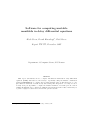
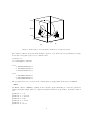
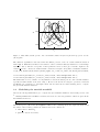
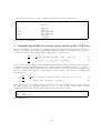
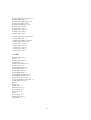
Figure 1: Both branches of the 1D unstable manifold of a saddle steady state.
Two initial conditions along the linear unstable eigenvector are then found by perturbing the saddle
steady state along this eigenvector by a distance dlta
>> dlta=0.01;
>> ic1=kt0p6stst.x+dlta*v
>> ic2=kt0p6stst.x-dlta*v
ic1 =
1.416441138941241e+00
-1.195381568105654e+00
7.647305114818007e+00
ic2 =
1.402293685085163e+00
-1.209517588934237e+00
7.647454996518048e+00
The program can now be executed at the command line by typing (while in the directory ManDde)
./GMRUN
(in Matlab, unix(’./GMRUN’)) resulting in the following output (including as a check the parameter
values) and required input; where we compute the unstable manifold corresponding to the initial condition
ic2
parameter
parameter
parameter
parameter
parameter
parameter
parameter
0:
1:
2:
3:
4:
5:
6:
0.6
3.57e-08
1.64e+08
1190
1.4e-12
3
2e-09
4
parameter 7: 0.0651
parameter 8: 1.6e-19
1. Unstable manifold of a fixed point.
2. Unstable manifold of a saddle periodic orbit.
Select option from menu:
1
Calculating a phase portrait
Please enter a file name:
pcfdemo/data/PCFic2.dat
Enter transient time (in tau):
0
Enter calculation time (in tau):
300
How many points to skip in output (in tau/n intervals):
50
Please give initial value for state 0:
1.402293685085163e+00
Please give initial value for state 1:
-1.209517588934237e+00
Please give initial value for state 2:
7.647454996518048e+00
After similarly computing the unstable manifold corresponding to the other initial condition ic1 we plot
the results (see Fig. 1 and stst plots.m)
>> load PCFic1.dat;
>> load PCFic2.dat;
>>
>>
>>
>>
>>
3
figure(1),clf,hold on, box on,axis square,view([50 15])
plot3(PCFic1(:,1),PCFic1(:,2),PCFic1(:,3),’r-’)
plot3(PCFic1(1,1),PCFic1(1,2),PCFic1(1,3),’r.’)
plot3(PCFic2(:,1),PCFic2(:,2),PCFic2(:,3),’b-’)
plot3(PCFic2(1,1),PCFic2(1,2),PCFic2(1,3),’b.’)
Unstable manifolds of saddle periodic orbits in the PCF laser
We now demonstrate how to compute 1D unstable manifolds of a saddle periodic orbit with one unstable
Floquet multiplier of the DDE describing the PCF laser; introduced in Section 2. To compute a 1D
unstable manifold of a saddle periodic orbit we first need, as starting data, initial conditions of length τ
along the saddle periodic orbit and along the unstable eigenfunctions on either side of the orbit [4]. The
manifold is then computed as a sequence of points of length τ with headpoints in a suitable section Σ
transverse to the flow. The distance between computed points is governed by four accuracy parameters,
αmin , αmax , (∆α)min and (∆α)max , where α denotes the approximate angle between three consecutive
points and ∆ is the distance between two successive points on the manifold. To reduce the number of
bisection steps in a calculation a small parameter ε is specified. To identify and adjust for tangencies to
the flow with Σ, during a computation, the integration time between consecutive points on the manifold
is tracked. We allow a given difference in the integration time between two such points. A computation
stops when convergence to a fixed point is detected, an end tangency is detected or when a prescribed
arclength of the manifold is reached; see Ref. [7] for full details.
5
7.66
0.8
N
ℑ(µ)
7.62
7.58
0
−0.8
−2
0
E
2
−1
0
1
2
ℜ(µ)
x
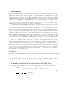
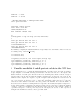
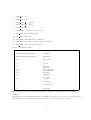
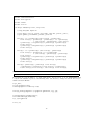
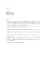
Figure 2: Left: Saddle periodic orbit A shown in projection onto the (Ex , N )-plane. The plane of intersection
Σ ≡ {(E, N ) | N = 7.62} is indicated by a dashed line, the end of the periodic profile is indicated by the large
dot. Right: Stability information.
3.1
Computing the starting data
We will assume that we have computed a branch of periodic orbits from which we have extracted a
saddle periodic orbit with a single unstable Floquet multiplier, namely kt2p500psol.mat. This file can
be found in the subdirectory pcfdemo in which we start Matlab. A bifurcation analysis involving this
saddle periodic orbit can be found in Ref. [3]. We first initialise the system and load this orbit into
Matlab. We call this orbit A; it is shown along with its stability information in Fig 2; see psol script.m
and psol plots.m.
>> sys_init;
>> load kt2p500psol.mat;
>> A=kt2p500psol;
>>
>>
>>
>>
>>
>>
>>
figure(2),clf
subplot(1,2,1),box on,hold on,axis square
plot(A.profile(1,:),A.profile(3,:),’k-’,’LineWidth’,1)
plot(A.profile(1,end),A.profile(3,end),’k.’,’MarkerSize’,15)
plot([-3.5 3.5],[7.62 7.62],’k--’,’LineWidth’,1)
subplot(1,2,2),box on,hold on,axis square
p_splot(A)
Now that we have the saddle periodic orbit A we use Matlab to compute the starting data. For this we
need to define some parameters:
1. The state variable as first defined in sys rhs.m; this defines the plane of intersection Σ
>> sec_coord = 3;
2. The value of Σ; see Fig. 2 (left)
>> sec_value = 7.62;
6
3. The size of the delay τ
>> tau = 1.0;
4. The number of subintervals in a delay interval
>> nn = 2500;
5. The perturbation δ applied to the eigenfunction
>> pert = 0.02;
6. A real value fm in the complex plane for which we want to compute the eigenfunction associated
with the Floquet multiplier with modulus greater than fm; see Fig. 2 (right)
>> fm = 1.7;
7. As the orbit intersects Σ a number of times, in our case 20 times, the intersection point for which
we want to compute the unstable manifold
>> intsn = 19;
The next step is to phase-shift the periodic orbit A so that the end point of its profile lies in the plane
Σ at the appropriate intersection point. This is done using the function find spo.m and the following
user-defined DDE-BIFTOOL extra condition sys cond.m. We denote the shifted orbit by C.
function [resi,condi]=sys_cond(point)
% xx: A B NN
% par: kt delta epsilon NO GN taup alpha taue II q Escale Nscale tauscale tau
if point.kind==’psol’
% fix endpoint at NN = 7.62
resi(1)=point.profile(3,end)-7.62;
condi(1)=p_axpy(0,point,[]);
condi(1).profile(3,end)=1;
else
error(’SYS_COND: point is not psol’);
end;
return;
>> method=df_mthod(’psol’);
>> [B,C,A0] = find_spo(A,sec_coord,sec_value,tau,nn,intsn,method);
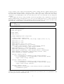
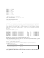
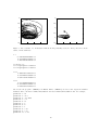
From the periodic orbit C we extract the initial condition of length τ with headpoint in the section Σ
using the function convert data.m. The resulting initial condition D1, shown in Fig. 3, is written to the
given file, in this case data/spokt2p5int19.dat.
>> D1 = convert_data(C,sec_coord,sec_value,tau,nn,’data/spokt2p5int19.dat’);
>>
>>
>>
>>
>>
figure(3);clf,hold on,box on,axis square
plot(C.profile(1,:),C.profile(3,:),’k-’,’LineWidth’,1)
plot([-3.5 3.5],[7.62 7.62],’k-’,’LineWidth’,1)
plot(D1(1,:),D1(3,:),’k-’,’LineWidth’,4)
plot(D1(1,end),D1(3,end),’k.’,’MarkerSize’,24)
7
7.66
N
7.62
7.58
−2
0
Ex
2
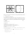
Figure 3: Phase shifted saddle periodic orbit C and initial condition D1 (in bold) shown in projection onto the
(Ex , N )-plane.
The unstable eigenfunction associated with the shifted periodic orbit C is obtained with the function
find eigd.m. This function finds both branches of the local linear unstable manifold of C and manipulates the data so that the end points of their profiles lie in Σ; see Ref. [4] for details. Again we use
convert data.m to extract two further initial conditions of length τ along this local unstable manifold.
>> [E,F,G1,G2,G2a,H1,H2,newvec]=find_eigd(C,sec_coord,sec_value,tau,nn,fm,pert,method);
>> I1=convert_data(H1,sec_coord,sec_value,tau,nn,’data/e1kt2p5int19.dat’);
>> I2=convert_data(H2,sec_coord,sec_value,tau,nn,’data/e2kt2p5int19.dat’);
The small value of δ is too small to see any difference between the saddle periodic orbit C and the unstable
eigendirections H1 and H2 on the scale of Fig. 3. However, the user is encouraged to plot these orbits and
use Matlab’s zoom function to investigate them. We now have the necessary starting data to compute
the global 1D unstable manifold.
3.2
Globalising the unstable manifold
We now use the algorithm in Ref. [7] to compute the global unstable manifold of the saddle periodic orbit
C.
With SystemPar.dat and RHS.cc defined as in Section 2, the new parameter values are given in the
file Parameters.dat as
2.5 3.57e-8 1.64e8 1190.0 1.4e-12 3.0 2.0e-9 65.1e-3 1.6e-19
The next step is to edit the file GrowingManifoldData.dat containing input and output information and
the values of the accuracy parameters outlined in Section 3. These are
1. first delta - initial ∆k
2. epsilon - bisection tolerance
8
3. alpha max - αmax
4. alpha min - αmin
5. delta alpha max - (∆α)max
6. delta alpha min - (∆α)min
7. delta min - ∆min
8. convergence - convergence to fixed point
9. sec coord - state in which Σ lies
10. sec value - value of Σ
11. arclength - maximum length of manifold
12. intersections - number of intersections of C with Σ
13. time fudge - integration time tolerance
see Ref. [7] for further details.
pcfdemo/data/spokt2p5int19.dat
InputFile1
pcfdemo/data/e1kt2p5int19.dat
InputFile2
pcfdemo/data/man1kt2p5int19.dat
OutputFile1
5.0e-4
first_delta
0.2
epsilon
0.3
0.2
1.0e-3
1.0e-4
1.0e-2
1.0e-4
alpha_max
alpha_min
delta_alpha_max
delta_alpha_min
delta_min
convergence
2
7.62
sec_coord
sec_value
5.5
arclength
20
intersections
0.3
time_fudge
The program can now be executed by typing at the command line (while in the directory ManDde)
./GMRUN
Alternatively, execute in Matlab using unix(’./GMRUN’). As a check, we output to screen the values of
the parameters, the file in which the manifold data will be written and the section value
9
parameter
parameter
parameter
parameter
parameter
parameter
parameter
parameter
parameter
0:
1:
2:
3:
4:
5:
6:
7:
8:
2.5
3.57e-08
1.64e+08
1190
1.4e-12
3
2e-09
0.0651
1.6e-19
1. Unstable manifold of a fixed point.
2. Unstable manifold of a saddle periodic orbit.
Select option from menu:
2
pcfdemo/data/man1kt2p5int19.dat
Section value: 7.62
Check correct branches are being computed:
Continue? ’y or n’
y
To check that one is computing the correct branch of the manifold, ten iterations of the local Poincaré
map are performed. The data is stored in the file pcfdemo/data/man1kt2p5int19.dat. This can be
plotted, the result giving an indication as to whether or not you want the manifold computation to
continue. Typing y, the output file will be overwritten with the data computed using the algorithm.
Typing n, the program will exit. Assuming we wish to continue, the option of displaying screen output
will be made
Display screen output? ’y or n’
y
+8.7394633e-01 +2.6296566e+00
+8.5604148e-01 +2.6326061e+00
+8.5260698e-01 +2.6333790e+00
+8.5208801e-01 +2.6334573e+00
+8.5109899e-01 +2.6336061e+00
+8.4930729e-01 +2.6338749e+00
+8.4542921e-01 +2.6344525e+00
+7.6200000e+00
+7.6200000e+00
+7.6200000e+00
+7.6200000e+00
+7.6200000e+00
+7.6200000e+00
+7.6200000e+00
FP
ED
IOPP
Algm
Algm
Algm
Algm
+1
+2
+3
+4
+5
+6
+7
+1.8146162e-02
+1.8146162e-02
+1.8646162e-02
+1.9646162e-02
+2.1646162e-02
+2.5646162e-02
+3.3646162e-02
giving the value of the intersection of the manifold with Σ (also written to
pcfdemo/data/man1kt2p5int19.dat), the number of points computed along the manifold and the arclength.
The algorithm exits after 75 points have been calculated, with an arclength of 1.818, after convergence
to a fixed point is detected with the message
Attractor reached through convergence!
To compute the other, longer branch of the manifold we change the input and output files in
GrowingManifoldData.dat to
pcfdemo/data/spokt2p5int19.dat
InputFile1
pcfdemo/data/e2kt2p5int19.dat
InputFile2
pcfdemo/data/man2kt2p5int19.dat
OutputFile1
and run ./GMRUN again. This time the program breaks after an arclength of 5.5 has been reached with
the message
10
Ey
2.9
2.6
2.3
−1
0
1
2
Ex
Figure 4: Both branches of the 1D unstable manifold of the saddle fixed point (+).
Prescribed arclength reached!
Exit? ’y or n’
If y is selected the program will exit. If n is selected the following message is displayed and the maximum
arclength can be increased to, for example, 6.0
n
Increase the arclength to:
6
We now use Matlab to plot the computed manifold
>>
>>
>>
>>
>>
>>
>>
>>
>>
>>
>>
figure(4),clf,hold on,box on,axis square
load data/man1kt2p5int19.dat
plot(man1kt2p5int19(:,1),man1kt2p5int19(:,2),’k-’,’LineWidth’,1)
plot(man1kt2p5int19(:,1),man1kt2p5int19(:,2),’b.’,’MarkerSize’,6)
plot(man1kt2p5int19(1,1),man1kt2p5int19(1,2),’k+’,’MarkerSize’,15,’LineWidth’,2)
plot(man1kt2p5int19(end,1),man1kt2p5int19(end,2),’kx’,’MarkerSize’,15,’LineWidth’,2)
load data/man2kt2p5int19.dat
plot(man2kt2p5int19(:,1),man2kt2p5int19(:,2),’k-’,’LineWidth’,1)
plot(man2kt2p5int19(:,1),man2kt2p5int19(:,2),’r.’,’MarkerSize’,6)
plot(man2kt2p5int19(1,1),man2kt2p5int19(1,2),’k+’,’MarkerSize’,15,’LineWidth’,2)
plot(man2kt2p5int19(end,1),man2kt2p5int19(end,2),’kx’,’MarkerSize’,15,’LineWidth’,2)
11
To check the accuracy [7] of these computations change the accuracy parameters to
1.0e-4
first_delta
0.2
epsilon
0.3
0.2
5.0e-4
5.0e-5
5.0e-3
5.0e-5
alpha_max
alpha_min
delta_alpha_max
delta_alpha_min
delta_min
convergence
and recompute the manifolds.
4
Unstable manifolds of external-cavity modes in the COF laser
We now demonstrate a special case of computing 1D unstable manifolds in systems with rotational S 1 symmetry [9]. Namely, the Lang-Kobayashi (LK) equations describing a semiconductor laser subject to
conventional optical feedback (COF). These equations can be written as [6]
dE
dt
dN
dt
=
1
GM0 (1 + iα) (N (t) − NN ) E(t) + κE(t − τ ) exp [−iCp ]
2
=
J0 − γ0 N (t) − [ΓM0 + GN0 (N (t) − NN )] |E(t)|
2
(2)
(3)
for the evolution of the complex electric field E(t) and the inversion N (t) [6]. Equations (2) and (3) have
S 1 -symmetry under the transformation (E, N ) → (cE, N ) where the symmetry group S 1 = {c ∈ C | |c| =
1}. When computing unstable manifolds of the LK-equations, we exploit their rotational symmetry and
write the complex electric field in a rotating frame of reference E(t) = A(t) exp(ibt) [5] resulting in the
following system
dA
dt
dN
dt
=
1
GM0 (1 + iα) (N (t) − NN ) A(t) − ibA(t) + κA(t − τ ) exp [−i(Cp + bτ )]
2
=
J0 − γ0 N (t) − [ΓM0 + GN0 (N (t) − NN )] |A(t)| .
2
(4)
(5)
In this way, periodic solutions (known as external cavity modes of the COF laser) appear as steady states.
We will compute an unstable manifold of one of these saddle steady states; namely
cofdemo/cp31p5stst.mat. First we must define the system in C++ as follows
3
0.22
2500
dimension
tau
subintervals
with right-hand side
12
#include "ClassDefinitions.h"
#include "GlobalVariables.h"
#include "Prototypes.h"
#include <cmath>
#include <vector>
void Datapt::RHS(Datapt first, Datapt last)
{
// Lang-Kobayashi Equations
// par0:kappa, par1:Cp, par2:bb, par3:alpha, par4:GM0, par5:N0, par6:J0,
// par7:gamma0, par8:GammaM0, par9:GN0, par10:tau
state[0] = 0.5 * parameter[4] *(last.state[2] - parameter[5])
* last.state[0] + (parameter[2] - parameter[3] * 0.5 * parameter[4]
* (last.state[2] - parameter[5])) * last.state[1]
+ parameter[0] * cos(parameter[1] + parameter[2] * parameter[10])
* first.state[0]
+ parameter[0] * sin(parameter[1] + parameter[2] * parameter[10])
* first.state[1];
state[1] = 0.5 * parameter[4] * (last.state[2] - parameter[5])
* last.state[1] + (parameter[3] * 0.5 * parameter[4]
* (last.state[2] - parameter[5]) - parameter[2])
* last.state[0]
+ parameter[0] * cos(parameter[1] + parameter[2] * parameter[10])
* first.state[1]
- parameter[0] * sin(parameter[1] + parameter[2] * parameter[10])
* first.state[0];
state[2] = parameter[6] - parameter[7] * last.state[2]
- (parameter[8] + parameter[9] * (last.state[2] - parameter[5]))
* (last.state[0] * last.state[0] + last.state[1] * last.state[1]);
}
and parameters
25.0 31.5 -51.85278770791984 3.5 50.0 5.0 8.0 1.0 0.55 0.05 0.22
After writing the new file RHS.cc, recompile using make. As in Section 2, we use DDE-BIFTOOL
to compute the unstable eigenvector and starting data. We therefore, change the current directory to
cofdemo and start Matlab.
>> sys_init;
>> load cp31p5stst.mat;
>> lbda=cp31p5stst.stability.l1(1)
>> A0=sys_deri(cp31p5stst.x,cp31p5stst.parameter,0,[],[]);
>> A1=sys_deri(cp31p5stst.x,cp31p5stst.parameter,1,[],[]);
>> tau=cp31p5stst.parameter(11);
>> Delta=A0+A1*exp(-lbda*tau);
>> [v,e]=eig(Delta)
>> v=v(:,3)
13
6
6
5.5
5.5
5
5
4.5
4.5
4
4
3.5
0
2
4
6
3.5
8
0
2
4
6
8
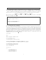
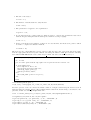
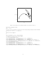
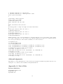
Figure 5: Two branches of a 1D unstable manifold showing bistability between a fixed point and a chaotic
attractor in the COF laser.
v =
-5.546346744963866e-01
8.230244811552463e-01
1.225197178637979e-01
>> dlta=0.01;
>> ic1=cp31p5stst.x+dlta*v
>> ic2=cp31p5stst.x-dlta*v
ic1 =
2.488933150761937e+00
8.230244811552464e-03
4.679107519514766e+00
ic2 =
2.500025844251865e+00
-8.230244811552464e-03
4.676657125157490e+00
We execute the program ./GMRUN (or in Matlab unix(’./GMRUN’)) as before and output the unstable
manifold data to the files cofdemo/data/COFic1.dat and cofdemo/data/COFic2.dat. For example,
parameter
parameter
parameter
parameter
parameter
parameter
parameter
parameter
parameter
parameter
parameter
0: 25
1: 31.5
2: -51.8528
3: 3.5
4: 50
5: 5
6: 8
7: 1
8: 0.55
9: 0.05
10: 0.22
14
1. Unstable manifold of a fixed point.
2. Unstable manifold of a saddle periodic orbit.
Select option from menu:
1
Calculating a phase portrait
Please enter a file name:
cofdemo/data/COFic1.dat
Enter transient time (in tau):
0
Enter calculation time (in tau):
50
How many points to skip in output (in tau/n intervals):
5
Please give initial value for state 0:
2.488933150761937e+00
Please give initial value for state 1:
8.230244811552464e-03
Please give initial value for state 2:
4.679107519514766e+00
Taking advantage of the rotational symmetry of the LK-equations, we plot the intensity |A(t)| against
N ; see Fig. 5 and Refs. [6, 9]. One branch of the unstable manifold is clearly seen to spiral down and
into a fixed point while the other branch accumulates on a chaotic attractor.
>>
>>
>>
>>
>>
>>
>>
>>
>>
>>
>>
>>
>>
figure(5);clf
load data/COFic1.dat
load data/COFic2.dat
A(:,1)=sqrt(COFic1(:,1).*COFic1(:,1)+COFic1(:,2).*COFic1(:,2));
B(:,1)=sqrt(COFic2(:,1).*COFic2(:,1)+COFic2(:,2).*COFic2(:,2));
subplot(1,2,1),box on,hold on,axis square
plot(A(:,1),COFic1(:,3),’b-’)
plot(A(1,1),COFic1(1,3),’kx’,’MarkerSize’,12,’LineWidth’,2)
axis([0 8 3.5 6])
subplot(1,2,2),box on,hold on,axis square
plot(B(:,1),COFic2(:,3),’r-’)
plot(B(1,1),COFic2(1,3),’kx’,’MarkerSize’,12,’LineWidth’,2)
axis([0 8 3.5 6])
Acknowledgements
My thanks go to Bernd Krauskopf for collaboration in developing the manifold algorithm, Jan Sieber for
testing the code, and Pieter De Ceuninck for helpful discussions.
Appendix A: List of files
System definitions
GrowingManifoldData.dat
Parameters.dat
SystemPar.dat
15
pcfdemo/Parameters_PCF.dat
pcfdemo/RHS_PCF.cc
pcfdemo/SystemPar_PCF.dat
pcfdemo/kt0p6stst.mat
pcfdemo/kt2p480psol.mat
pcfdemo/sys_cond.m
pcfdemo/sys_deri.m
pcfdemo/sys_init.m
pcfdemo/sys_rhs.m
pcfdemo/sys_tau.m
cofdemo/Parameters_COF.dat
cofdemo/RHS_COF.cc
cofdemo/SystemPar_COF.dat
cofdemo/cp31p5stst.mat
cofdemo/sys_cond.m
cofdemo/sys_deri.m
cofdemo/sys_init.m
cofdemo/sys_rhs.m
cofdemo/sys_tau.m
C++ files
AdamsIntegrator.cc
Bisect.cc
ClassDefinitions.h
CopyCDList.cc
CreateListFromFile.cc
FindInterval.cc
FindingCandidate.cc
GlobalVariables.cc
GlobalVariables.h
GrowingManifold.cc
GrowingManifoldData.cc
GrowingManifoldHeader.cc
InterpolateToSection.cc
IterationOfPoincarePoint.cc
ListManipulation.cc
Main.cc
Makefile
Parameters.cc
PhasePortrait.cc
PoincareStep.cc
Prototypes.h
RHS.cc
SectionCheck.cc
SuperPoincare.cc
SystemPar.cc
16
Matlab files
convert_data.m
find_eigd.m
find_spo.m
pcfdemo/psol_plots.m
pcfdemo/psol_script.m
pcfdemo/stst_plots.m
pcfdemo/stst_script.m
cofdemo/stst_plots.m
cofdemo/stst_script.m
References
[1] K. Engelborghs, T. Luzyanina, and G. Samaey. DDE-BIFTOOL v2.00: a Matlab package for bifurcation analysis of delay differential equations. Technical Report TW-330, Department of Computer
Science, K. U. Leuven, Belgium, 2001. http://www.cs.kuleuven.ac.be/~koen/delay/ddebiftool.shtml.
[2] K. Green and B. Krauskopf. Global bifurcations at the locking boundaries of a semiconductor laser
with phase-conjugate feedback. Phys. Rev. E, 66(016220), 2002.
[3] K. Green, B. Krauskopf, and K. Engelborghs. Bistability and torus break-up in a semiconductor laser
with phase-conjugate feedback. Phys. D, 173:114–129, 2002.
[4] K. Green, B. Krauskopf, and K. Engelborghs. One-dimensional unstable eigenfunction and manifold
computations in delay differential equations. J. Comput. Phys., 2004, to appear.
[5] B. Haegeman, K. Engelborghs, D. Roose, D. Pieroux, and T. Erneux. Stability and rupture of
bifurcation bridges in semiconductor lasers subject to optical feedback. Phys. Rev. E, 66(046216),
2002.
[6] T. Heil, I. Fischer, W. Elsäßer, B. Krauskopf, K. Green, and A. Gavrielides. Delay dynamics of
semiconductor lasers with short external cavities: Bifurcation scenarios and mechanisms. Phys. Rev.
E, 67(066214), 2003.
[7] B. Krauskopf and K. Green. Computing unstable manifolds of periodic orbits in delay differential
equations. J. Comput. Phys., 186:230–249, 2003.
[8] B. Krauskopf and H. M. Osinga. Growing 1d and quasi-2d unstable manifolds of maps. J. Comput.
Phys., 146:404, 1998.
[9] B. Krauskopf, G. H. M. Van Tartwijk, and G. R. Gray. Symmetry properties of lasers subject to
optical feedback. Opt. Commun., 177:347–353, 2000.
17