Download Field Survey of Wireless ISM-band Channel Properties for

Field Survey of Wireless ISM-band Channel
Properties for Substation Applications
Alireza Shapoury, Student Member IEEE, and Mladen Kezunovic, Fellow IEEE
Abstract- During this field survey, we measured and
recorded a few quality parameters of wireless
communication in a substation switchyard. A
microprocessor-based measurement system was used for
data collection and analysis. We investigated long-term
noise variation in this specific environment. Based on our
measurement and post-processing analysis we conclude
that the so-called Classic/Bayesian assumption of existing
noise distributions appear not to be a suitable all-round
model for analysis. Variations in bandwidth occupancy
patterns of other wireless devices sharing the same
frequency and many other factors necessitate updated
measurements and post processing. We noticed dominant
underlying structure in noise profiles, which calls for a
comprehensive time series analysis. Given the stationarity
of the data set and the Wold’s theorem, An Auto
Regressive Moving Average (ARMA) model can be found
for the data set with similar behaviors.
Keywords- Communication systems, Power transmission
electromagnetic interference, Substation measurements, Time
Series, Wireless LAN.
I. INTRODUCTION
commercial application of wireless communications
VAST
has required comprehensive theoretical and practical
studies in this area. Except for limited applications like
satellite communication, the channels are identified to be
interference-limited due to the multiplicity of wireless devices
in the corresponding spectrum.
The magnitude and the effect of ambient noise juxtaposed
to interferences differ from a place/time to another. Several
measurements have been comprehensively conducted since 35
years ago in this regard [1],[2]. On-going technological
changes, channel utilizations, atmospheric impacts and other
parameters necessitates frequent and updated field
measurement and comprehensive analysis campaign. This
analysis might suggest considerable changes to the man-made
noise model, which is presently used in a radio link design.
Proximity, power settings, number of the wireless devices
in the network and even choosing modulation and coding
format closely depend on the magnitude of noise and
interference impacts. For instance if the channel is identified
as an interference- limited channel, increasing the power
This work was sponsored by Power Systems Engineering Research Center
(PSERC), National Science Foundation Industry/University Collaborative
Research Center.
A. Shapoury and M. Kezunovic are with the Department of Electrical
Engineering, Texas A&M University, College Station, TX 77843-3128,
Email:{shapoury, kezunov}@ee.tamu.edu.
setting would not improve the link quality, while power
setting is a crucial factor in noise-limited channels [3] (If we
double the transmission power level from all wireless devices,
they will cause twice as high interference level, leaving us
with the same Signal-to-Interference ratio, and thus the same
bit-error probability.)
In here we narrow down our analysis to substation noise
impacts on 900MHz ISM frequency bands. (ISM stands for
the Industry, Scientific, and Medical [4]).
A measurement setup has been formed to enable longperiod test runs in different substation yards to inspect the
long-time impact of substation noise on the wireless channels.
The variations of the noise profile in the substation have been
closely observed and discussed in this survey.
II. MEASUREMENT SETUP
The proposed setup consisted of two radio transceivers.
Fig. 1 shows typical dispositions of the transceivers. Two
processing units (Fig. 2) were deployed and programmed to
emulate the continuous data communication to the virtual
circuit breaker and to handle the logging and background
processing.
The in-yard radio was installed 1.2m above the ground
level and electrically attached/grounded to the metallic
structures of the circuit breaker. Since the wireless
communication analysis is aimed at monitoring operation of
circuit breakers, we considered free-body metering [5]
inappropriate in this case. Our measurement setup was subject
to calibration error. We ignored this offset error, as the general
methodology adopted is invariant to this offset error and the
background noise may induce offset in different locations.
The survey duration of our measurement run was about 14
days in 345 KV yard to include weather cycle extremes and
probable diurnal and weekly patterns. The noise calculations
were done as a moving average of 256 readings during each
frequency hop spread over 902 to 928MHz frequency
spectrum (Each reading is about a 20 ms and the sample
interval is approximately 5 seconds.) If multiple samples are
taken at the same frequency in the time period, the most recent
sample is most significant with a weight of 256 and a value
that had been sampled 255 samples back will have a weight of
one. The average noise was calculated and recorded each oneminute using the above procedure. Hence there are more than
20,000 observations per our dataset.
The processing unit also handled the data logging. Sensors
recorded the body-temperatures of the instruments. This
enabled us to check any probable correlation of the ambient
temperature and our readings.
Fig. 2. Master radio data device and the diagnostic
computer
Many of the radio engineers adopted the Bayesian
approach, as there already exist some underlying assumptions
about the radio propagation and noise profiles in the literature.
The validity of the scientific conclusions becomes intrinsically
linked to the validity of these underlying assumptions. In
practice since some of the assumptions are unknown or
untested for specific applications, the validity of the scientific
conclusions becomes suspect.
In the next part, we probe our measurement results. We
will see that there is no appropriate distributional modeling to
this problem. Hence we base our analysis in the rest of the
survey on exploratory approach. This method also requires
fewer encumbering assumptions.
Fig. 1. Equipment disposition
(a) Master transceiver, which is attached to the control room, is
connected to the logging device (b) and (c) Slave radios, connected
to the metallic body of the circuit breaker
The instruments have negligible or no correlation to the
temperature deviation within the nominal range [6].
II. METHODOLOGY
There are basically three popular data analysis approaches
that we can adopt here: Classical, Bayesian and Exploratory
Data Analysis. The difference among these approaches which
all yield to engineering conclusions is the sequence and focus
of the intermediate steps.
For the Classical approach a model is first defined and the
analysis is based on this model. For a Bayesian analysis, dataindependent distribution is imposed on the parameters of the
selected model according to the engineering knowledge of the
analyst. Then the observed data and the a-priori knowledge
about the distribution on the parameters are incorporated to
construct interval estimates of the model parameters or even to
validate the collected data. Finally, in the exploratory data
analysis approach, the analyst focuses on finding the best-fit
model to the collected data by discovering the behavioral
patterns of the gathered data.
IV.NOISE ANALYSIS
In wireless system designs, the probability that the noise
exceeds a threshold level is crucial. In general, a model is
defined by experience and theoretical conjecture for noise and
its distribution identifies the above-mentioned probability.
Then the maximum difference between the empirical and the
hypothetical cumulative distributions are measured by some
test statistics. This test is called “test of goodness of fit”.
In the Classical and Bayesian methodology as mentioned
before an a-priori (distributional) model is defined before the
analysis. In our case, nonetheless, it is basically hard to
identify a hypothetical distribution in the first place, which
copes with the empirical data. A suggested noise distribution
of a typical substation is discussed in [2]. The suggested
statistics depends upon the value of certain parameters in the
noise distribution. The multiplicity of the parameters involved
in this model and the complexity of extracting them using
long test runs while maintaining small time resolution, make it
practically intricate to define an all-round appropriate
hypothetical noise distribution for a substation.
From the measurement point of view, hypothesis testing is
readily performed if the observations are normally distributed.
(Based on the central limit theorem, the observations are
therefore assumed as normally distributed.)
Usually the assumption of normal distribution of the
observation for the parameter estimation is checked by these
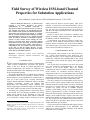
V. STATISTICAL CONFIDENCE
OF THE RESULTS
IEEE recommendation for site survey suggests using
Kolmogorov-Smirnov method to calculate the statistical
confidence of the measurement [8]. This approach works only
when the Cumulative Distribution Function (CDF) is
reasonably continuous.
In practical measurement, we do not always have the
luxury of having both a high-resolution measuring device and
a large dynamic range, which is required for impulsive noise
measurement. If we decrease the dynamic range to have a
better resolution then we miss the impulses that may occur.
This trade-off is the source of our discontinuities in
Cumulative Distribution Function. The other way to work
around the problem is to use Moving Average (MA) technique
to make a practically continuous cumulative distribution.
Fortunately, our measurement setup allows long duration
survey and consequently large size for our data set (more than
14000 data samples per each data set). With such data
redundancy we might expect to achieve observation values in
the vicinity of the average values of the actual data.
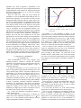
Fig. 3 shows the Cumulative Distribution Function of
345KV substation yard.
For large sample sizes N (bigger than 35 samples), the
critical value of the distribution is defined as dα ( N ) / N in
which dα ( N ) is the maximum absolute difference between
sample and population cumulative distribution.
1
Cumulative Distribution Function (CDF)
hypothesis tests. Such an approach is problematic, if the
estimates of the parameters are used to compute the theoretical
normal distribution. If the estimates are falsified by the model
deviations, then this already can be a reason for deviation
from a normal distribution.
There are other tests, which get along without the
assumption of a special distribution with which the test of a
general linear hypothesis is not possible. In these tests the
sampling distribution depends neither on explicit form of nor
the value of certain parameters in distribution model. These
test are called non-parametric or distribution free tests in the
sense that the critical values do not depend on the specific
distribution being tested. By means of goodness-of-fit tests
such as chi-squared test and Kolmogorov-Smirnov test,
empirical or assumed univariate distributions can be compared
with theoretical or hypothetical univariate distributions, for
instance the univariate normal distribution. KolmogorovSmirnov (K-S) test has been considered to be the most
appropriate tool for our scenario among other non-parametric
tests [7]. This is the method, which has been suggested by
IEEE [8]. Statisticians however prefer to use the modified K-S
test; the Anderson-Darling [9] (A-D) test. A-D improves the
K-S test by granting more weight to the tail of the distribution
in the fit model than to its midrange, which allows a more
sensitive test especially to fat tail distributions. The A-D test
has the disadvantage that the critical values should be
calculated for each distribution; however, this drawback is less
intense since the tables of critical values are readily available
and are usually applied with statistical software programs [9].
0.9
Γ = 16.84 (The slope at X i=X m )
0.8
0.7
0.6
0.5
0.4
0.3
0.2
0.1
0
8
9
10
11
12
13
14
15
16
17
× 10 8
Observed Result
Fig. 3. Cumulative Distribution Function (CDF) of the
measured data
For instance if a %90 confidence is desired, i.e. the
significant level ( α ) of 0.10, the maximum absolute deviation
between the sample cumulative distribution and the population
cumulative distribution will be at least dα ( N ) / N . In other
words, we can say that the calculated median X m is expected
to lie within ± dα ( N ) /(Γ N ) of the true population median
with %90 confidence. In the same vein, we can any take other
values of X i and run the same calculation for that point.
This is a measure of the confidence in our data and the
results are independent from the form of the distribution
function which characterizes the observe data [7].
Table I gives the calculated confidence percentage of our
survey according to this method. The small value of the
deviation from the actual median is due to the large sample
size in our case (more than 14,000 samples). Hence according
to this analysis we can be almost sure about the confidence of
our results.
Table I Expected Deviation With Respect To The Confidence
Levels For 900MHz Measurement
Confidence Level
Expected Deviation
from the median
%80
%90
%99
5.37
6.12
8.18
× 10
−4
× 10
−4
× 10
−4
The only drawback of this method is the difficulties in the
calculation of the slope of the Cumulative Distribution
Function at the data point of interest. This is usually
implemented graphically rather than analytically.
In the next part we will show that unfortunately there are
some fundamental problems that make this analysis
questionable. We still keep this part as an effort to follow
IEEE recommendations on the site survey.
Let’s now probe our data to see if the results basically
suggest the use of distributional measures discussed above.
One of the basic assumptions in determining whether a
process is stochastic or deterministic is randomness. If the
process is stochastic, each data value may be viewed as a
sample mean of a probability distribution of the underlying
population at each point in time. If the assumptions of
randomness, fixed distribution, and constant scale and location
are satisfying then we can model a univariate process as:
ωi = χ + εi ,
where ω i is the observed variable, χ is the underlying
data-generating process or the source data, and ε i is an error
term.
If the randomness assumption of a process is violated, then
we shall typically use a different model such as time series.
We can then identify the stochastic and deterministic
components in the process.
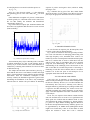
Fig. 4 shows the run sequence plot. It indicates that the data
do not have any significant shifts in location or scale over time
(hence stationary).
sequence of positive and negative values, which are mildly
decaying to zero.
Fig. 6 indicates the lag plot of the data, which further
shows the presence of a few outliers in our data set. The above
plots reject an appropriate distribution model for our dataset.
-8
2.4
x 10
2.2
2
Noise Voltage (Uncalibrated)
1.8
1.6
Fig. 6. Lag Plot
1.4
VI. GRAPH INTERPRETATIONS
1.2
1
0.8
0.6
0
0.2
0.4
0.6
0.8
1
1.2
1.4
1.6
Samples
1.8
2
4
x 10
Fig. 4. Run Noise Sequence Plot of Voltage
Autocorrelation plots [10] are commonly used as a measure
to indicate randomness in a data set (the formula, which is
used in [10], is in autocovariance sense). This randomness is
examined by evaluating autocorrelations for observed values
at different time lags.
The sample autocorrelation (autocovariance) plot (Fig. 5)
shows that the time series is not random, but rather has a high
degree of autocorrelation between adjacent and near-adjacent
observations. Since the randomness assumption is thus
seriously violated, the distribution approach is ignored since
determining the distribution of the data is only meaningful
when the data are random. The plot exhibits an alternating
Fig. 5. Sample Autocorrelation Plot
As seen from the run sequence plot, the data points, taken
over time, seem to have an internal structure.
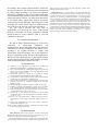
Fig. 7 shows recorded noise values for typical days of these
two weeks. The data have an underlying pattern along with
some high frequency noise, meanwhile there seems to be
neither any obvious seasonal pattern in the data nor data points
that are so extreme that we need to delete them from the
analysis. These types of non-random data can be modeled
using time series methodology. We first have to obtain an
understanding of the underlying forces and structure of the
data set and then fit a model and proceed to forecasting or
monitoring or both. We observe that the data set is an almost
trend-free set. In the next parts we will attempt to fit an
appropriate model based on the data structure.
VII. UNIVARIATE TIME SERIES
Time series may be stationary or non-stationary. Many
statistical analysis techniques are based on the assumption that
the data are stationary. However, we can often transform the
non-stationary time series into a stationary series either by
taking the natural log, differencing or by taking residuals from
a regression and then stabilizing the variance across time.
Although seasonality also violates stationarity, we can usually
apply a seasonal adjustment and render it amenable to time
series analysis.
In our case, run sequence shows almost constant location
and scale and there does not seem to be a significant trend.
Sharp peaks also indicate that the ARMA model is more
successful than the window estimation (e.g. Parzen window)
[11], hence we adopt ARMA modeling approach. Based on
the Wold’s decomposition theorem any stationary process can
be approximated by an ARMA model (although this model
might not be found easily). Once we fit the model we shall
inspect the residual to ensure that it has a Gaussian
than one, may be appropriate for these data. The partial
autocorrelation plot should be examined to determine the
order.
The partial autocorrelation plot (Fig. 8) suggests that an
AR(8) model might be appropriate (since the amplitude
becomes negligible at 8th lag). Hence our initial attempt is to
fit an AR(8) model. Model validation rejects this model since
the resulting residuals fail to have a random Gaussian
distribution. On the other hand the presence of peaks and
trough in the run sequence plot suggest ARMA models as
another potential fit. We adopt this more generalized model
here from now on.
(a)
Fig. 8. Partial Autocorrelation Plot
(b)
(c)
Fig. 7. Recorded Noise Values For Typical Days of These Two
Weeks
distribution. This would justify the goodness of our fit.
Box and Jenkins [10] introduced a systematic approach and
developed an algorithmic methodology for identifying and
estimating ARMA models. We shall also deploy this
systematic approach to model our dataset. Then the next step
is to determine the order of the autoregressive and moving
average terms in the Box-Jenkins model. After fitting the
model, we should validate the time series model. The primary
tool for validating the model is residual analysis.
VIII. MODEL IDENTIFICATION
The autocorrelation plot (Fig. 5) shows a mixture of
exponentially decaying and damped sinusoidal components.
This indicates that an autoregressive model, with order greater
First, we use Akaike’s Information Criterion to find a full
AR model [11]. We use readymade statistical software for this
purpose. An AR(27) model will fit our data best.
Second, we use stepwise ARMA method to look for subset
AR and obtain the alpha coefficient.
It suggest a AR(21) model with AIC=-4744.27 to be a
better fit than full AR model. Third, we use stepwise ARMA
method to look for a subset ARMA model we achieve p=36
q=24 (i.e. the orders of our ARMA model) having an
AIC = -4812.06 , which is less than full AR model. Now we
need to estimate our model’s parameters and find the
residuals. We use the Marquardt algorithm to calculate the
MLE for the parameters of our model [11]. We get: -1.0174,
0.6803, -0.3740, 0.0726, -0.0306, -0.0377, -0.3446, -0.9222,
and 0.3474. These are our α1 , α 2 , α 3 , α17 , α 29 , α 36 , β 3 ,
β 21 , and β 24 .
IX- MODEL VERIFICATIONS
Now we have to check the residuals of our model, if these
residuals are white noise, then the chosen model is judged to
be a proper fit. Using Q-test we got p-value of 0.07361. Hence
we don’t have significant evidence rejecting the hypothesis
that the residuals are white noise. Hence ARMA (36,24) is our
final model. If we fail to receive a residue of Gaussian noise,
we shall redo the procedure afresh to achieve better ARMA
model.
X. CONCLUSION
The characteristics of the dataset that we gathered from the
substation site survey, indicates that the classical distributional
analysis is not an appropriate approach for prediction. The
measured data has a strong non-random component with long-
time memory and a stationary internal structure, which calls
for time series analysis. This structured can be modeled with
an ARMA model according to the Wold’s decomposition
theorem[12]. Although the order of the ARMA model might
become ultimately high, prediction can be easily calculated by
off-the-shelf statistic software. The observation and analysis
of the measured data suggest (time sensitive) site-specific
wireless design for this application. Considering this a-priori
knowledge, the wireless system analyst can optimize the best
time of the day/week for on-site wireless network analysis.
The next research direction will focus first on
understanding and identifying the causes of the internal
structures in the dataset and on the comparison of different
measured dataset in several substation yards to verify the
conformity of the results.
XI. ACKNOWLEDGEMENTS
We wish to thank CenterPoint Energy Co. for its active
cooperation
in
measurement
installations
and
implementations. We also thankfully acknowledge the active
contribution of FreeWave Technologies and Alvarion Ltd in
providing us the required provisions to conduct some
measurements using their products. We are also indebted to
Professor Longnecker and Mr. Weimin of the Department of
Statistics at Texas A&M University for their helpful guidance
on processing recorded field data, which furnished us with the
ability and the momentum to complete this work.
XII. REFERENCES
[1]
Achatz, R.J., et al, “Man-Made Noise in the 136 to 138-MHz VHF
Meteorological Satellite Band”, NTIA Report 98-355, 10998.
[2] Riley, N.G. and Docherty, K. “Modeling and measurement of man-made
radio noise in the VHF-UHF Band,” Proc. Of the Ninth Internat. Conf.
On Ant. Prop., vol. 2. Pp. 313-316.
[3] Simon, M.K., Omura J. K., Scholtz R. A., Levitt B. K., “Spread
Spectrum Communications Handbook”, McGraw-Hill, 2002.
[4] 47 CFR, PART 15 -Radio Frequency Devices, Federal Communications
Commission (FCC), last updated on August 20, 2002.
[5] IEEE standard procedures for the measurement of radio noise from
overhead power lines and substations, ANSI/IEEE Std 430-1986.
February 28, 1986
[6] Multipoint Diagnostic Program User Manual, FreeWave Technologies
[7] MASSEY, Jr, FRANK J. The Kolmogorov-Smirnov Test for Goodness
of Fit. American Statistical Association Journal, Mar 1951, pp 68–78.
[8] IEEE recommended practice for an electromagnetic site survey (10 kHz
to 10 GHz) IEEE Std 473-1985, 18 June 1985.
[9] Stephens, M. A. EDF Statistics for Goodness of Fit and Some
Comparisons, Journal of the American Statistical Association, Vol. 69,
pp. 730-737, 1974.
[10] Box, G. E. P., G. M. Jenkins and G. C. Reinsel; Time Series Analysis,
Forecasting and Control. 3rd ed. Prentice Hall, Englewood Clifs, N.J.,
1994.
[11] Newton, H.J., TIMESLAB, A Time Series Analysis Laboratory,
Wadsworth & Brooks/Cole, 1988
[12] H. O. Wold, A Study in the Analysis of Stationary Time Series, Alquist
and Wiksell, Uppsala, Sweden, 1938.
XII. BIOGRAPHIES
Alireza Shapoury (S’00) received his B.E and M.E. degrees from
Beheshti University and the University of Science and Technology in Iran, in
1994 and 1997 respectively, all in electronic engineering.
He worked at Beheshti University as a lecturer from 1997 through 1999.
Since June 2000, he has been with Texas A&M University pursuing his Ph.D.
degree. His main research interests are radio propagation, wireless testing
techniques and autonomous systems.
Mladen Kezunovic (S’77, M’80, SM’85, F’99) received his Dipl. Ing.
Degree from the University of Sarajevo, the M.S. and Ph.D. degrees from the
University of Kansas, all in electrical engineering, in 1974, 1977 and 1980,
respectively. Dr. Kezunovic’s industrial experience is with Westinghouse
Electric Corporation in the USA, and the Energoinvest Company in Sarajevo.
He also worked at the University of Sarajevo. He was a Visiting Associate
Professor at Washington State University in 1986-1987. He has been with
Texas A&M University since 1987 where he is the Eugene E. Webb Professor
and Director of Electric Power and Power Electronics Institute. His main
research interests are digital simulators and simulation methods for equipment
evaluation and testing as well as application of intelligent methods to control,
protection and power quality monitoring. Dr. Kezunovic is a registered
professional engineer in Texas, and a Fellow of IEEE.