Download PAPPU-THESIS

DESIGN AND ANALYSIS OF WIND ENERGY SYSTEMS IN POWER
APPLICATIONS
by
Santosh Pappu, B.E
A Thesis
In
ELECTRICAL ENGINEERING
Submitted to the Graduate Faculty
of Texas Tech University in
Partial Fulfillment of
the Requirements for
the Degree of
MASTER OF SCIENCES
IN
ELECTRICAL ENGINEERING
Approved
Dr. Stephen B Bayne
Chair of Committee
Dr. Michael Giesselmann
Peggy Gordon Miller
Dean of the Graduate School
August, 2012
Copyright 2010, Santosh Pappu
Texas Tech University, Santosh Pappu, August 2012
ACKNOWLEDGMENTS
I am grateful to Dr. Stephen Bayne for taking me as a graduate student early in
my Masters. He has been a guide in every senses. His thoughts and insights to
Electrical Engineering have only broadened my horizon in Electrical Engineering. His
ideas and guidance have been instrumental in publishing three IEEE conference papers
during my time here. His belief in my abilities and constant encouragement has made
me work harder to achieve my goals.
I would like to thank Dr. Michael Giesselmann for accepting to be the co-chair
on my committee for my thesis defense.
I thank Mr. Jerry Lopez for being a great mentor. He has been an inspiration
throughout my Masters. His work ethics and commitment has been a great influence
on me. Interacting with him has only made me a better person.
I thank my friends Chaitanya S.K, Purvi Patni and Sanjar Hussain for
encouraging me throughout my Masters. I thank Mr. Sandeep Nimmagadda for
helping me with my research and internship.
I thank Srividya for being my pillar of strength throughout my Masters.
Without her it wouldn’t have been possible to survive the day to day hardships of life
in USA.
Lastly I would like to thank my parents and Almighty from the bottom of my
heart for giving me the opportunity to study in the United States. Without their
blessings none of this would have been possible.
ii
Texas Tech University, Santosh Pappu, August 2012
TABLE OF CONTENTS
ACKNOWLEDGMENTS ............................................................................................ ii
ABSTRACT .............................................................................................................. v
LIST OF TABLES .................................................................................................... vi
LIST OF FIGURES .................................................................................................. vii
CHAPTER
I. INTRODUCTION .................................................................................................... 1
1.1 Introduction to Wind Energy ........................................................................ 1
1.1.1 Wind Turbines ................................................................................................... 1
1.1.2 Generators ........................................................................................................ 2
1.2 Wind Energy Technologies ........................................................................... 3
1.3 Introduction to Comparison of Wind Turbines with Different Power Ratings
............................................................................................................................. 4
1.4 Introduction to Hub Concept......................................................................... 4
1.5 Introduction to Power Quality....................................................................... 4
1.6 MATLAB ...................................................................................................... 5
II. THEORETICAL BACKGROUND ........................................................................... 6
2.1 Energy Conversion ....................................................................................... 6
2.2 Generators Used in the Wind Industry .......................................................... 7
2.2.1 Singly Fed Induction Generator ........................................................................ 7
2.2.2 Doubly Fed Induction Generator ....................................................................... 8
2.2.3 Synchronous Generator .................................................................................. 10
2.2.4 Permanent Magnet Generator ........................................................................ 11
2.3 Wind Turbine Technologies........................................................................ 12
2.3.1 Type 1 ............................................................................................................. 12
2.3.2 Type 2 ............................................................................................................. 13
2.3.3 Type 3 ............................................................................................................. 14
2.3.3 Type 4 ............................................................................................................. 15
2.4 STATCOM.................................................................................................. 16
iii
Texas Tech University, Santosh Pappu, August 2012
III. EVALUATION OF HUB CONCEPT FOR WIND TURBINES ................................ 20
3.1 Designation of Hubs.................................................................................... 21
3.2 Technical Analysis for Designation of Hubs .............................................. 21
IV. MODEL DEVELOPMENT PROCEDURE ............................................................ 23
4.1 Wind Profile ................................................................................................ 23
4.2 Induction Generator Model in MATLAB ................................................... 25
4.3 Doubly Fed Induction Generator Model in MATLAB ............................... 27
4.4 STATCOM.................................................................................................. 29
4.5 Topology of Wind Farms For Comparison of Wind Farms........................ 31
4.6 Topology of Wind Farms for Hub Concept ................................................ 32
V. POWER QUALITY ANALYSIS USING PHASOR MEASUREMENT UNIT .............. 34
5.1 Power Quality Issues ................................................................................... 34
5.2 SEL 421 ...................................................................................................... 37
5.3 Synchrophasor Vector Processor-SEL 3378 .............................................. 38
5.4 SVP Configurator ....................................................................................... 39
5.5 SEL SynchroWave Archiver ..................................................................... 41
5.6 SEL SynchroWave Console ....................................................................... 41
5.7 Point of Connection of PMU ..................................................................... 43
5.8 Baseline of Parameters of Power Flowing into the Facility ....................... 43
5.9 Description of Code for Power Quality Analysis ...................................... 44
VI. RESULTS FOR COMPARITIVE STUDY OF WIND TURBINES ............................ 47
6.1 Wind Speeds ranging from 3-6m/s ............................................................. 47
6.2 Wind Speeds ranging from 9-12m/s ........................................................... 49
6.3 Wind Speeds ranging from 21-24m/s ......................................................... 52
6.4 Equal Power Lost ........................................................................................ 54
6.5 Equal Number of Turbines Lost to Faults ................................................... 56
VII. RESULTS FOR EVALUATION OF HUB CONCEPT ........................................... 59
7.1 Rated Conditions ......................................................................................... 59
7.2 Fault on One Wind Turbine in Wind Farm ................................................. 60
7.3 Fault on Wind Farm A ................................................................................ 63
VIII. RESULTS FOR POWER QUALITY ANALYSIS USING A PMU........................ 65
IX. CONCLUSION .................................................................................................. 68
X. FUTURE WORK................................................................................................. 71
REFERENCES ......................................................................................................... 72
PUBLICATIONS ...................................................................................................... 74
iv
Texas Tech University, Santosh Pappu, August 2012
ABSTRACT
Advance Research was conducted in Wind Energy. It was divided into various
categories of wind energy. The areas of research are comparison between mid size and
large size wind turbines, power quality analysis and the evaluation of hub concept for
wind turbines. The characteristics of two wind farms of the same power capacity
having two different size generators were compared. The research compared the
performance of mid-size turbines to large turbines. The systems were modeled in
MATLAB-Simulink. A 9MW wind farm consisting of eighteen Fixed Speed Induction
Generators (FSIG) with STATCOM at the terminals of the wind farm was compared
to a 9MW wind farm consisting of six Doubly Fed Induction Generators (DFIG. An
analysis on total power available for transmission, reactive power consumption at
different wind speeds (cut in, rated, cut off), power loss due to loss of turbines was
done.
The next part of the research involved transient response of three wind farms
interconnected to the grid at the same point designated as Hub, rated 9MW each was
modeled and simulated. Each wind farm consists of six Doubly Fed Induction
generator turbines rated at 1.5MW each, interfaced with power electronics on the rotor
side. The model was modeled in MATLAB-Simulink. Analysis on voltage stability of
wind farms due to faults on the neighboring wind farm was done.
A novel approach to record and analyze the power coming from the utility was
devised. A Phasor Measurement Unit (PMU) was set up located at a Semiconductor
Foundry Fabrication Facility (sensitive load) for analysis of the Power Quality of the
Facility. A code was developed for filtering the data collected from the PMU in
MATLAB. A GUI developed in MATLAB analyzed the data from the PMU and
highlights aberrations in the values of Voltages and Frequency from the Power Quality
limits for sensitive loads. A unique method for analysis of Power Quality before the
installation of a wind turbine directly feeding the Facility so as to set a standard after
the wind turbine is installed.
v
Texas Tech University, Santosh Pappu, August 2012
LIST OF TABLES
4.1
Parameters of Induction Generator. ............................................................. 34
4.2
Parameters of DFIG ..................................................................................... 36
5.1
Common Power Quality Issues .................................................................... 42
vi
Texas Tech University, Santosh Pappu, August 2012
LIST OF FIGURES
1.1
Offshore Wind Turbine. ................................................................................. 8
1.2
Generator of a Wind Turbine. ...................................................................... 10
2.1
Squirrel Cage Induction Generator Connected to grid. ................................ 15
2.2
Doubly Fed Induction Generator Connected to grid. ................................... 16
2.3
Schematic of Syncrhonous Generator . ........................................................ 17
2.4
Permanent Magent Generator Connected to grid. ........................................ 18
2.5
Fixed Speed Wind Turbine Generator Connected to grid. ........................... 19
2.6
Type 2 Wind Turbine Connected to grid. .................................................... 21
2.7
Type 3 Wind Turbine. .................................................................................. 22
2.8
Type 4 Wind Turbine. .................................................................................. 22
2.9
STATCOM connected to a transmission line. ............................................. 23
2.10
Equivalent Circuit of STATCOM. ............................................................... 24
2.11
Waveforms of Current and Voltage. ............................................................ 25
4.1
Various Wind Speeds used in Simulation. ................................................... 31
4.2
Model of Induction Generator in MATLAB Simulink. ............................... 32
4.3
Feedback loop for Pitch Angle Control. ...................................................... 33
4.4
Model of the DFIG in MATLAB. ................................................................ 35
4.5
Schematic of STATCOM............................................................................. 37
4.6
Topology of Wind Turbines connected in a Wind Farm. ............................ 39
4.7
Schematic of wind farms for Hub Concept. ................................................. 40
5.1
Schematic of SEL 421 connected using CT’s and PT’s. ............................. 45
5.2
System Configuration of SEL 3378. ............................................................ 46
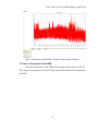
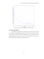
5.3
Plot from Synchrowave Console of Current in Phase C. ............................. 49
5.4
Line diagram showing point of connection of PMU. ................................... 50
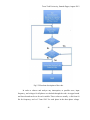
5.5
Flowchart description of the code. ............................................................... 52
5.6
GUI developed in MATLAB. ...................................................................... 53
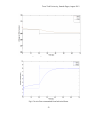
6.1
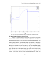
Reactive Power consumption for both wind farms for
wind speeds ranging from 3-6m/s. ............................................................... 55
6.2
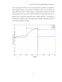
Active Power transmission for wind speeds ranging from
3-6m/s........................................................................................................... 56
vii
Texas Tech University, Santosh Pappu, August 2012
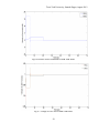
6.3
Reactive Power consumption for both wind farms. ..................................... 57
6.4
Voltage at 25kV bus for both wind farms. ................................................... 58
6.5
Active power transmitted from both wind farms ......................................... 58
6.6
Reactive Power consumed for both wind farms. ......................................... 60
6.7
Voltage at 25 kV for both wind farms. ........................................................ 60
6.8
Active Power generated for wind speeds from 21-24m/s. ........................... 61
6.9
Reactive Power consumption for a three phase fault for
01.sec............................................................................................................ 62
6.10
Active Power Transmitted when 1.5MW is lost in both
wind farms. ................................................................................................... 63
6.11
Active Power transmitted to the grid from both wind
farms ............................................................................................................. 64
6.12
Electrical Torque of both generators when a three phase to
ground fault occurs. ...................................................................................... 65
7.1
Active Power at point of interconnection..................................................... 67
7.2
Voltage at terminals of wind turbine with three phase to
ground fault. ................................................................................................. 68
7.3
Voltage at terminals of wind farm B. ........................................................... 69
7.4
Electrical Torque of wind turbine in wind farm B. ...................................... 70
7.5
Terminal Voltage of Wind Farm A. ............................................................. 71
8.1
GUI display when there is an excursion in the parameters. ......................... 72
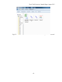
8.2
Folder where the erroneous files are saved. ................................................. 73
8.3
Sub folder where the waveforms and excel sheet
containing the data are saved ....................................................................... 74
viii
Texas Tech University, Santosh Pappu, August 2012
CHAPTER 1
INTRODUCTION
1.1 Introduction to Wind Energy
Wind energy is gaining increasing importance throughout the world. This fast
development of wind energy technology and of the market has large implications for a
number of people and institutions, electrical engineers at universities. For wind turbine
manufacturers, and for developers of wind energy projects, who also need that
understanding in order to be able to develop feasible, modern and cost-effective wind
energy projects [1].
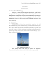
1.1.1 Wind Turbines
A wind turbine is a device that converts kinetic energy from the wind
into mechanical energy. If the mechanical energy is used to produce electricity, the
device may be called a wind generator. Wind turbines are designed to exploit the wind
energy that exists at a location. Aerodynamic modeling is used to determine the
optimum tower height, control systems, number of blades and blade shape [2]. Fig 1.1
shows an offshore wind turbine.
Fig.1.1 Offshore Wind Turbine [2]
Wind turbines convert wind energy to electricity for distribution.
Conventional horizontal axis turbines can be divided into three components [2]:
1
Texas Tech University, Santosh Pappu, August 2012

The rotor component, which is approximately 20% of the wind turbine cost,
includes the blades for converting wind energy to low speed rotational energy.

The generator component, which is approximately 34% of the wind turbine
cost, includes the electrical generator, the control electronics, and most likely
a gearbox
(e.g. planetary
gearbox, adjustable-speed
drive or continuously
variable transmission) component for converting the low speed incoming
rotation to high speed rotation suitable for generating electricity.

The structural support component, which is approximately 15% of the wind
turbine cost, includes the tower and rotor yaw mechanism [2].
Small wind turbines may be used for a variety of applications including on- or
off-grid residences, telecom towers, offshore platforms, rural schools and clinics,
remote monitoring and other purposes that require energy where there is no electric
grid, or where the grid is unstable.
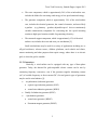
1.1.2 Generators
Basically, a wind turbine can be equipped with any type of three-phase
generator. Today, the demand for grid-compatible electric current can be met by
connecting frequency converters, even if the generator supplies alternating current
(AC) of variable frequency or direct current (DC). Several generic types of generators
may be used in wind turbines [1]:

. Asynchronous (induction) generator:

squirrel cage induction generator (SCIG)

wound rotor induction generator (WRIG)

Doubly-fed induction generator (DFIG)

. Synchronous generator:

wound rotor generator (WRSG)

Permanent magnet generator (PMSG)
2
Texas Tech University, Santosh Pappu, August 2012
Fig.1.2 Generator of a Wind Turbine [3]
Fig 1.2 shows the stator and rotor of a generator of a turbine. The rotor of the
wind turbine is connected to the rotor of the generator via a shaft or gear box. The
rotation of the blades of the wind turbine causes rotation of the rotor which in turn
rotates the rotor of the generator. This mechanical energy is converted to electrical
energy which is supplied to the grid.
1.2 Wind Energy Technologies
Wind Turbine technologies can be classified according to type of speed control
and power control. Currently four different types of technologies exist. They vary in
terms of generators used and additional equipment used for speed and power control.
The four types are

Type 1: Induction Generator directly connected to the grid from the stator. This
is also known as fixed speed generator since the frequency of the stator is same
as the grid frequency.

Type 2: Variable speed turbine connected to the grid directly. The speed can be
varied by varying the rotor resistance.

Type 3: These are Doubly Fed Induction Generators which are variable speed.
The rotor is connected to the grid via power electronics. This makes both the
stator and rotor feed power to the grid.

Type 4: These types of generators are connected to the grid via the power
electronics. The stator of the generator is connected to the power electronics
which in turn is connected to the grid. These are variable speed wind turbines
[1].
3
Texas Tech University, Santosh Pappu, August 2012
In this research, we have considered two types of generators. Those are type 1 and
type 3 wind turbines.
1.3 Introduction to Comparison of Wind Turbines with Different Power
Ratings
In this research, two wind farms consisting of 9MW each are compared. The
two wind farms differ in the turbine being used. One wind farm has eighteen singly
fed induction generators each rated at 500 kW and the other wind farm consists of six
doubly fed induction generators each rated at 1.5 MW. The two wind farms have been
simulated for various wind speeds and transient stability. The performances of both
the wind farms have been analyzed for the above said conditions and parameters such
as voltage, active power and reactive power have been monitored.
1.4 Introduction to Hub Concept
Currently the interconnection of multiple wind farms on the same
transmission line is being debated by some of the Regional Transmission
Organizations (RTO) such as Southwest Power Pool (SPP). The point of
interconnection is being designated as the Hub.
The Generation Interconnection
process in the tariff allows each Generation Interconnection Customer to identify a
transmission line or station on the transmission system to interconnect with. It was
recommended that multiple generators connect at one point on a line rather than at
multiple points because it is more efficient, reliable and cost effective [4].
Research was conducted to analyze the impact of transients on wind farms
simulated modeled around the Hub concept. A description about the Hub concept has
been included in Chapter 3. The wind farms were simulated for faults at various
locations and active power, reactive power and voltage at the bus were monitored for
their respective cases.
1.5 Introduction to Power Quality
Power Quality is the set of limits of electrical properties that allows electrical
systems to function in their intended manner without significant loss of performance
or life. The term is used to describe electric power that drives an electrical load and the
4
Texas Tech University, Santosh Pappu, August 2012
load's ability to function properly with that electric power. Without the proper power,
an electrical device (or load) may malfunction, fail prematurely or not operate at all.
There are many ways in which electric power can be of poor quality and many more
causes of such poor quality power. While "power quality" is a convenient term for
many, it is the quality of the voltage rather than power or electric current that is
actually described by the term.
Today wind-generating system is connected into the power system to meet the
consumer’s demand. The addition of wind power into the electric grid affect’s the
power quality. Due to the increase awareness of power quality particularly in highly
sensitive industry like continuous process industry, complex machine part producing
industry and security related industry where standardization and evaluation of
performance is an important aspect [5].
1.6 MATLAB
Though different software were used for this research, primarily the modeling
for the wind turbines for comparative study and evaluation of hub concept were done
in MATLAB. The modes were built and simulated in MATLAB Simulink and Sim
Power Systems.
For archiving the data being recorded from the Phasor Measurement Unit
(PMU), Synchrowave Archiver was used. SVP configurator was used to initialize the
PMU. Synchrowave Console was used to capture the instantaneous values of voltage,
current and frequency as a plot with respect to time.
5
Texas Tech University, Santosh Pappu, August 2012
CHAPTER 2
THEORETICAL BACKGROUND
There are four different types of generators used in the wind industry out of
which two have been used in this research. A brief description about all the four types
of generators and the technologies they are associated is also discussed. The theory
behind the conversion of energy from mechanical to electrical is also discussed to give
a better understanding.
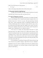
2.1 Energy Conversion
The aerodynamic blades on the rotor convert the kinetic energy of the wind
into mechanical energy, effectively providing the torque Tr on the rotor:
(2.1)
Where
angular speed of rotor and power is Pr and is given by the following
relation:
(2.2)
ρ is the air density, R the wing radius and v the effective wind speed.
is the
efficiency coefficient which is a function of the blade pitch angle θ and the tip speed
ratio ʎ. In the context of this project, ʎ is the ratio between the blade tip speed and the
wind speed.
λ=
Where
(2.3)
is the speed at the tip of the blade. However the inverse ratio is also
commonly met in the literature. The performance coefficients cp for wind turbines are
obtained through numerical calculations and look-up tables.
Assuming the generator is lossless, the total power is transferred from the rotor of the
wind turbine to the generator. Hence rotor power would be equal to electrical power
generated.
(2.4)
6
Texas Tech University, Santosh Pappu, August 2012
where
is the electrical power of the generator.
(2.5)
where
is the torque of the generator and
is the generator speed.
2.2 Generators Used in the Wind Industry
Presently in the Wind Industry four different types of generators are being for
power generation. All the four types have been discussed below.
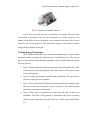
2.2.1 Singly Fed Induction Generator
The most common generator used in wind turbines is the induction generator.
It has several advantages, such as robustness and mechanical simplicity and, as it is
produced in large series, it also has a low price. The major disadvantage is that the
stator needs a reactive magnetizing current. The asynchronous generator does not
contain permanent magnets and is not separately excited. Therefore, it has to receive
its exciting current from another source and consumes reactive power. The reactive
power may be supplied by the grid or by a power electronic system. The generator’s
magnetic field is established only if it is connected to the grid.
In the case of AC excitation, the created magnetic field rotates at a speed
determined jointly by the number of poles in the winding and the frequency of the
current, the synchronous speed. Thus, if the rotor rotates at a speed that exceeds the
synchronous speed, an electric field is induced between the rotor and the rotating
stator field by a relative motion (slip), which causes a current in the rotor windings.
The interaction of the associated magnetic field of the rotor with the stator field results
in the torque acting on the rotor.
So far, the Squirrel Cage Induction Generator (SCIG) has been the prevalent
choice because of its mechanical simplicity, high efficiency and low maintenance
requirements. The SCIG is directly coupled to grid. Hence this is normally used in
Fixed Speed configuration as the generator frequency and grid frequency should
match for synchronism [1].
7
Texas Tech University, Santosh Pappu, August 2012
Fig 2.1 Squirrel cage Induction Generator connected to the grid on the stator and wind
turbine on the rotor [6].
Fig.2.1 shows the schematic of the singly fed induction generator. The rotor of
the generator is connected to the rotor of the turbine. The stator is directly coupled to
the grid.
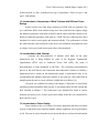
2.2.2 Doubly Fed Induction Generator
The Doubly Fed Induction Generator (DFIG) comes under the category of
Wound Rotor Induction Generators (WRIG). In the case of a WRIG, the electrical
characteristics of the rotor can be controlled from the outside, and thereby a rotor
voltage can be impressed. The windings of the wound rotor can be externally
connected through slip rings and brushes or by means of power electronic equipment,
which may or may not require slip rings and brushes. By using power electronics, the
power can be extracted or impressed to the rotor circuit and the generator can be
magnetized from either the stator circuit or the rotor circuit. It is thus also possible to
recover slip energy from the rotor circuit and feed it into the output of the stator. The
disadvantage of the WRIG is that it is more expensive than the SCIG and not as robust
as the SCIG.
8
Texas Tech University, Santosh Pappu, August 2012
The DFIG consists of a WRIG with the stator windings directly connected to
the constant-frequency three-phase grid and with the rotor windings mounted to a
bidirectional back-to-back IGBT voltage source converter. The term ‘doubly fed’
refers to the fact that the voltage on the stator is applied from the grid and the voltage
on the rotor is induced by the power converter. This system allows a variable-speed
operation over a large, but restricted, range. The converter compensates the difference
between the mechanical and electrical frequency by injecting a rotor current with a
variable frequency. Both during normal operation and faults the behavior of the
generator is thus governed by the power converter and its controllers. The power
converter consists of two converters, the rotor-side converter and grid-side converter,
which are controlled independently of each other [1].
Fig.2.2 Rotor of the DFIG connected through the power electronics to the grid and the
stator is connected directly to the grid [7].
Fig.2.2 shows the schematic of a DFIG. The rotor of the generator is connected
to the grid through the power electronics. The stator of the generator is connected
directly to the grid. This implies that the stator needs to operate at grid frequency and
the rotor can operate at variable frequency due to the power electronics interface.
9
Texas Tech University, Santosh Pappu, August 2012
2.2.3 Synchronous Generator
The synchronous generator is much more expensive and mechanically more
complicated than an induction generator of a similar size. However, it has one clear
advantage compared with the induction generator, namely, that it does not need a
reactive magnetizing current.
The magnetic field in the synchronous generator can be created by using
permanent magnets or with a conventional field winding. If the synchronous generator
has a suitable number of poles, it can be used for direct-drive applications without any
gearbox.
As a synchronous machine, it is probably most suited for full power control as
it is connected to the grid through a power electronic converter. The converter has two
primary goals: (1) to act as an energy buffer for the power fluctuations caused by an
inherently gusting wind energy and for the transients coming from the net side, and (2)
to control the magnetization and to avoid problems by remaining synchronous with the
grid frequency. Applying such a generator allows a variable-speed operation of wind
turbines [1].
Fig.2.3 Schematic of Synchronous Generator [8].
10
Texas Tech University, Santosh Pappu, August 2012
Fig.2.3 shows the schematic of the synchronous generator. The stator is
connected to the grid through the power electronics. The rotor is energized by DC
excitation. The rotor is connected to a rectifier for DC excitation.
The stator windings of WRSGs are connected directly to the grid and hence the
rotational speed is strictly fixed by the frequency of the supply grid. The rotor winding
is excited with direct current using slip rings and brushes or with a brushless exciter
with a rotating rectifier. Unlike the induction generator, the synchronous generator
does not need any further reactive power compensation system. The rotor winding,
through which direct current flows, generates the exciter field, which rotates with
synchronous speed. The speed of the synchronous generator is determined by the
frequency of the rotating field and by the number of pole pairs of the rotor.
2.2.4 Permanent Magnet Generator
In the permanent magnet (PM) machine, the efficiency is higher than in the
induction machine, as the excitation is provided without any energy supply. However,
the materials used for producing permanent magnets are expensive, and they are
difficult to work during manufacturing. Additionally, the use of PM excitation requires
the use of a full scale power converter in order to adjust the voltage and frequency of
generation to the voltage and the frequency of transmission, respectively. This is an
added expense [1].
Fig.2.4 Permanent Magnet Generator connected to the grid.
11
Texas Tech University, Santosh Pappu, August 2012
Fig.2.4 shows the synchronous generator connected to the grid through the
power electronics. However, the benefit is that power can be generated at any speed so
as to fit the current conditions. The stator of PMSGs is wound, and the rotor is
provided with a permanent magnet pole system and may have salient poles or may be
cylindrical. Salient poles are more common in slow-speed machines and may be the
most useful version for an application for wind generators. Typical low-speed
synchronous machines are of the salient-pole type and the type with many poles.
2.3 Wind Turbine Technologies
The electrical connection of wind turbines to the grid differs with the generator
type used. Currently four different technologies are prevalent for the four different
types of the generators discussed in the previous section. The four types will be
discussed in this section.
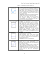
2.3.1 Type 1
This configuration denotes the fixed-speed wind turbine with an asynchronous
squirrel cage induction generator (SCIG) directly connected to the grid via a
transformer. Since the SCIG always draws reactive power from the grid, this
configuration uses a capacitor bank for reactive power compensation. A smoother grid
connection is achieved by using a soft-starter [1].
Fig.2.5 Fixed Speed Wind Turbine Generator connected directly to a grid.
12
Texas Tech University, Santosh Pappu, August 2012
Fig.2.5 shows the schematic of a type 1 technology wind turbine. The
generator is directly connected to the grid. For the purpose of synchronization the
generator is forced to run at a frequency of 60Hz. The capacitor bank is provided for
reactive power compensation.
Regardless of the power control principle in a fixed-speed wind turbine, the
wind fluctuations are converted into mechanical fluctuations and consequently into
electrical power fluctuations. In the case of a weak grid, these can yield voltage
fluctuations at the point of connection. Because of these voltage fluctuations, the
fixed-speed wind turbine draws varying amounts of reactive power from the utility
grid (unless there is a capacitor bank), which increases both the voltage fluctuations
and the line losses. Thus the main drawbacks of this concept are that it does not
support any speed control, it requires a stiff grid and its mechanical construction must
be able to tolerate high mechanical stress.
Type 1 wind turbines also consist of active pitch control type and stall control
type. Stall-controlled wind turbines cannot carry out assisted startups, which imply
that the power of the turbine cannot be controlled during the connection sequence.
They are popular because of its low price and simplicity.
The main advantages of active pitch control wind turbines are that it facilitates
power controllability, controlled startup and emergency stopping. Its major drawback
is that, at high wind speeds, even small variations in wind speed result in large
variations in output power. The pitch mechanism is not fast enough to avoid such
power fluctuations. By pitching the blade, slow variations in the wind can be
compensated, but this is not possible in the case of gusts.
2.3.2 Type 2
This configuration corresponds to the limited variable speed wind turbine with
variable generator rotor resistance. It uses a wound rotor induction generator (WRIG).
The generator is directly connected to the grid. A capacitor bank performs the reactive
13
Texas Tech University, Santosh Pappu, August 2012
power compensation. A smoother grid connection is achieved by using a soft-starter
[1].
Fig. 2.6 Type 2 Wind turbine directly connected to the grid.
Fig.2.6 shows the schematic of a type 2 wind turbine. It has variable additional
rotor resistance, which can be changed by an optically controlled converter mounted
on the rotor shaft. Thus, the total rotor resistance is controllable. This optical coupling
eliminates the need for costly slip rings that need brushes and maintenance. The rotor
resistance can be changed and thus controls the slip. This way, the power output in the
system is controlled. The range of the dynamic speed control depends on the size of
the variable rotor resistance. Typically, the speed range is 0–10%above synchronous
speed. The energy coming from the external power conversion unit is dumped as heat
loss.
2.3.3 Type 3
This configuration, known as the doubly fed induction generator (DFIG)
concept, corresponds to the limited variable speed wind turbine with a wound rotor
induction generator (WRIG) and partial scale frequency converter (rated at
approximately 30% of nominal generator power) on the rotor circuit . The partial scale
frequency converter performs the reactive power compensation and the smoother grid
connection. Typically, the speed range comprises 40% to 30 % of synchronous speed
14
Texas Tech University, Santosh Pappu, August 2012
[1]. The smaller frequency converter makes this concept attractive from an economical
point of view. Its main drawbacks are the use of slip rings and protection in the case of
grid faults.
Fig.2.7 Type 3 Wind Turbine.
Fig.2.7 shows the schematic of a type 3 wind turbine. The stator is directly
connected to the grid. The rotor is connected via the power electronics. This enables
the rotor to operate at variable speed. This also minimizes the voltage oscillations due
to mechanical oscillations on the rotor. The power electronics are rated for 30% of the
nominal power. This reduces the cost of power electronics.
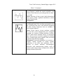
2.3.4 Type 4
This configuration corresponds to the full variable speed wind turbine, with the
generator connected to the grid through a full-scale frequency converter. The
frequency converter performs the reactive power compensation and the smoother grid
connection. The generator can be excited electrically or by a permanent magnet
permanent magnet synchronous generator [1].
Fig.2.8 Type 4 Wind Turbine.
15
Texas Tech University, Santosh Pappu, August 2012
Fig.2.8 shows the schematic of a type 4 wind turbine. The stator is isolated
from the grid in this configuration. The stator is connected to the grid through the
power electronics. Since the nominal power of the generator is transferred through the
power electronics, the switches need to be rated for full rating. This would increase the
cost of the power electronics, thereby increasing the total cost of the whole setup. The
power electronics enables the generator to run at variable frequency.
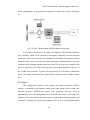
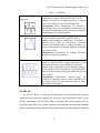
2.4 STATCOM
A STATCOM is a device connected in derivation, composed of a coupling
transformer that serves of as a link between the electrical power systems (EPS) and the
voltage synchronous controller (VSC). The VSC generates the voltage wave
comparing it to the one of the electric system to realize the exchange of reactive
power. The control system of the STATCOM adjusts at each moment the inverse
voltage so that the current injected in the network is in cuadrature to the network
voltage, in these conditions P=0 and Q=0.
In its most general way, the STATCOM can be modeled as a regulated voltage
source Vi connected to a voltage bar Vs through a transformer [9].
Fig.2.9 STATCOM connected to a transmission line [9].
16
Texas Tech University, Santosh Pappu, August 2012
The STATic COMpensator (STATCOM) uses a VSC interfaced in shunt to a
transmission line. In most cases the DC voltage support for the VSC will be provided
by the DC capacitor of relatively small energy storage capability - hence, in steady
state operation, active power exchanged with the line has to be maintained at zero, as
shown symbolically in Fig.2.9.
With the active power constraint imposed, the control of the STATCOM is
reduced to one degree of freedom, which is used to control the amount of reactive
power exchanged with the line. Accordingly, a STATCOM is operated as a functional
equivalent of a static VAR compensator; it provides faster control than an SVC and
improved control range [9].
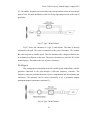
Fig.2.10 Equivalent Circuit of STATCOM [9].
17
Texas Tech University, Santosh Pappu, August 2012
Fig.2.10 shows the equivalent circuit of a STATCOM system. The GTO
converter with a dc voltage source and the power system are illustrated as variable ac
voltages in this figure. These two voltages are connected by a reactance representing
the transformer leakage inductance.
Using the classical equations that describe the active and reactive power flow
in a line in terms of Vi and Vs, the transformer impedance (which can be assumed as
ideal) and the angle difference between both bars, we can defined P and Q.
The angle between the Vs and Vi in the system is d. When the STATCOM
operates with d=0 we can see how the active power to the system device becomes zero
while the reactive power will mainly depend on the voltage module. This operation
condition means that the current that goes through the transformer must have a +/-90º
phase difference to Vs. In other words, if Vi is bigger than Vs, the reactive will be sent
to the STATCOM of the system (capacitive operation), originating a current flow in
this direction. In the contrary case, the reactive will be absorbed from the system
through the STATCOM (inductive operation) and the current will flow in the opposite
direction. Finally if the modules of Vs and Vi are equal, there won´t be nor current nor
reactive flow in the system.
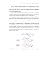
Fig.2.11 Waveforms of Current and Voltage for lagging and leading power factor [9].
18
Texas Tech University, Santosh Pappu, August 2012
Thus, we can say that in a stationary state Q only depends on the module
difference between Vs and Vi voltages. The amount of the reactive power is
proportional to the voltage difference between Vs and Vi.
There can be a little active power exchange between the STATCOM and the
EPS. The exchange between the inverter and the AC system can be controlled
adjusting the output voltage angle from the inverter to the voltage angle of the AC
system. This means that the inverter cannot provide active power to the AC system
form the DC accumulated energy if the output voltage of the inverter goes before the
voltage of the AC system. On the other hand, the inverter can absorb the active power
of the AC system if its voltage is delayed in respect to the AC system voltage.
19
Texas Tech University, Santosh Pappu, August 2012
CHAPTER 3
EVALUATION OF HUB CONCEPT FOR WIND TURBINES
Research was conducted for analysis of Hub Concept by building models of
wind farms in MATLAB based on the Hub Concept .The Southwest Power Pool (SPP)
is currently dealing with the Hub Concept. The committee responsible for the
allocation, designation of Hubs is the Area Generation Task Force. The Area
Generation Connection Task Force (AGCTF) is responsible for developing and
recommending policy to guide SPP Staff to determine the optimum method of
interconnecting generation given the complex situations generally prevalent [10].
The Hub Concept was initiated as Generation Developers are requesting
multiple interconnections on the same transmission line in close proximity to each
other. In addition to adding costs, having multiple interconnection substations in the
same geographical area can create many issues some of which are electrical, reliability
and aesthetics [10].
The Generation Interconnection process in the Tariff allows each Generation
Interconnection Customer (GIC) to identify a transmission line or station on the
transmission system to interconnect with. When a GIC elects to interconnect with a
transmission line, a new station must be built. GICs request that these new stations be
located at a point on the transmission line which minimizes the distance to their
generator. In addition, the inability of a subsequent generator developer to obtain
right-of-way across land that is already leased to an earlier developer may inhibit the
ability of the subsequent GIC to gain access to a transmission line or specific
substation. This leads the GIC to request an exclusive interconnection station at a
location which minimizes the length of the generator lead it needs to build utilizing the
right-of-way it can obtain. For solitary interconnection requests this is not an issue.
But in those areas where SPP has seen high concentration of interconnection requests
there can be many GIC’s requesting interconnection in the same geographical area,
each expecting its own new interconnection station [10].
20
Texas Tech University, Santosh Pappu, August 2012
3.1. Designation of Hubs
The AGCTF designates a specific new substation (Hub) in an area where
multiple generators are located as a single interconnection point. Hubs will only be
designated at 300kV or above. The establishment of a new Hub may be proposed by
SPP either through the Integrated Transmission Planning (ITP) process or the
Generation Interconnection process once two or more generators are proposing to
interconnect to the same transmission line in close proximity to each other. An
existing substation may be designated as a Hub for any new generation
interconnection requests in that vicinity. The designation of a Hub will result in more
certainty of the location of such generation collection substations.
The decision to propose the designation of a hub will be based on two different
analyses. The technical analysis will be based on a review of the transmission system
by SPP and the appropriate Transmission Owner and subsequent study to review
switching transients and whether switching transients are a concern. If the technical
studies determine that the addition of a new substation does not result in switching
transients that need to be controlled, then the second analysis based on economics will
be used. Here only the technical aspect of allocation of Hubs will be discussed.
3.2. Technical Analysis for Designation of Hubs
The AGCTF recommends that multiple generators connect at one point on a
line rather than at multiple points because it is more efficient, reliable, and cost
effective. Extremely long (over 75 miles) transmission lines that are tapped by
multiple generation interconnection substations may require the addition of line
reactors at each substation where the transmission line terminates. Line reactors are
required to limit transient switching voltages to a level that will not cause damage to
line switching equipment (circuit breakers) [10].
Destructive transients can be generated during normal switching operations,
thus requiring fixed line reactors to control these switching transients to a safe level.
Identifying the circumstances when these switching transients could occur requires
complex analysis, and the situation does not occur for all lines. For lines where
21
Texas Tech University, Santosh Pappu, August 2012
destructive switching surges are expected to occur, a transient analysis is necessary to
be performed to determine, among other things, the hub spacing; taking into
consideration the equipment needed to control switching surges, the increased cost of
the stations, and the effect fixed line reactors will have on line loadability [10].
Normally line reactors are installed on transmission lines to maintain voltages
on long lines during light loading conditions. When the line reactors are installed for
this reason they can be remotely disconnected from the transmission system during
times of heavy flows. If a reactor cannot be disconnected during times of heavy
loading, it can cause voltage depression and ultimately decrease safe line loading
capability [10].
In addition, each time a fixed shunt reactor is added to a line, the impedance of
the line increases. If enough fixed shunt reactors are added to a line, the increased
impedance can also reduce the amount of power that can flow down the line, thereby
reducing the amount of capacity available on the line for the normal movement of
power.
It is evident that interconnecting multiple generators at different points along a
single transmission line segment may degrade the reliability of the transmission
system [10].
22
Texas Tech University, Santosh Pappu, August 2012
CHAPTER 4
MODEL DEVELOPMENT PROCEDURE
In this chapter two wind farm topologies will be presented: a singly-fed
generator and a doubly fed induction generator along with the wind profiles for which
they have been simulated. The fixed speed wind farm has been compared to the DFIG
wind farm in various aspects. The development of wind farm transient models
provides an interesting insight into the performance of the topologies for disturbances
and fault conditions.
The model used for Evaluation of Hub Concept has also been discussed. First
the models for the comparison of wind farms with different configurations are
discussed and then models of the evaluation of Hub Concept are discussed.
4.1 Wind Profile
In this section the wind profile used in the model is discussed. For determining
the effect of wind generation on the electrical characteristics, it is only necessary to
translate the input wind speed into a mechanical torque, which is then applied to the
blades of the generator [11].
(4.1)
where
is the characteristic curve which depends on the generator,
the air density, R is the radius of the blades,
and
is the wind speed,
is
is the blade angle,
is the tip speed ratio, i.e. the ratio of the speed at the tip of the blades to the
speed of the wind, otherwise:
(4.2)
The wind farms have been simulated for three different wind profiles to
analyze the active power transmitted from the wind farm to the grid and reactive
power consumed for those wind profiles. The three wind profiles are at cut in wind
speed, at rated wind speed (where the turbines output maximum power) and at cut off
wind speed (where the turbines trip due to over speed condition). A PI controller has
23
Texas Tech University, Santosh Pappu, August 2012
been used to implement pitch angle control to limit the pitch angle of the blades of the
turbine. During high wind speeds, an over speed condition of the generators initiates a
trip
which
isolates
the
generator
from
the
rest
of
the
system.
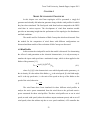
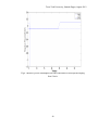
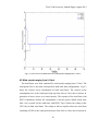
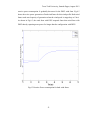
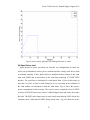
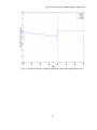
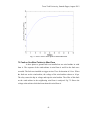
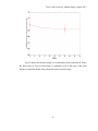
Fig.4.1 Various Wind Speeds used in the simulation for comparison of wind farms
with different configurations.
Fig.4.1 shows the graph depicting the wind speeds with respect to time. The
models were simulated for the three wind speeds. The three wind speeds are 3-6m/s,
9-12 m/s, 21-24 m/s. The wind speeds step up from the minimum value to the
maximum value at time 20sec. The two wind farms have been simulated for cut in,
rated and cut off wind speeds to compare the performance in aspects of

Reactive power consumed for different wind profiles.

Power transmitted to the grid taking transmission losses into account.

Steady state and dynamic performance of both the wind farm configurations
with equal number of turbines lost.

Steady state and dynamic performance of both the wind farm configurations
with equal power lost.
24
Texas Tech University, Santosh Pappu, August 2012
The simulation time considered is 50 seconds. The step change in wind speed is
considered to observe the response of the wind turbine to step changes in wind
speed.
4.2 Induction Generator Model in MATLAB
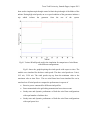
In MATLAB, the Induction Generator is represented using a wind torque
model, applied to the shaft of the Induction generator as shown in Fig.4.2. It also
contains a pitch angle control block which controls the pitch angle of the blades in
case of high wind speeds to limit the output power to the power rating of the machine.
The machine is initiated to a negative 1% slip to make it run in super synchronous
mode to generate power thereby not considering the sub-transients in the simulation.
Fig.4.2 Model of Induction Generator in MATLAB simulink [11].
25
Texas Tech University, Santosh Pappu, August 2012
Fig.4.2 shows the model of the induction generator in MATLAB Simulink.
The model is readily available in MATLAB. The model consists of a squirrel cage
induction generator connected to a circuit breaker on the stator. The model also
consists of a wind turbine model. The rotor of the turbine is connected to the rotor of
the generator. Wind speed is the input to the turbine. A feedback loop is designed for
the implementation of pitch angle control which is given as another input to the wind
turbine. Fig. 4.3 shows the feedback control used for pitch angle control.
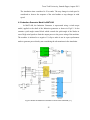
Fig.4.3 Feedback loop for Pitch Angle control [12].
In Fig.4.3, the nominal power is compared to the actual power from the
generator and given to the PI controller. The angle β is fed to the controls of the
turbine for pitch angle control. This pitch angle helps in the control of active power of
the wind turbine during high speeds. The mechanical torque
of the wind turbine
drives the rotor of the generator and is transferred as electrical torque
.
The circuit breaker connected to the stator of the generators receives trip
signals from a relay. The breaker trips the generator when the conditions such as over
voltage, over current over speed occur to shield the remaining power system from
damage. The relay sends a trip signal to the circuit breaker when it detects any of the
conditions mentioned before. Since the induction generator is modeled as a constant
26
Texas Tech University, Santosh Pappu, August 2012
current source a resistance is placed in parallel. The active power and reactive power
from the generator are measured from the voltage and current values measured using
the measurement blocks. The parameters used for the induction generator is shown
below in Table 4.1.
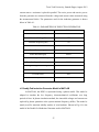
Table 4.1: PARAMETERS OF INDUCTION GENERATOR
Parameters
Values
Nominal Power(kW)
500kW
Nominal Voltage(V)
575
Nominal Frequency(Hz)
60
Nominal Power factor
0.9
Stator Resistance(pu)
0.0065
Rotor Resistance(pu)
0.0093
Stator Leakage inductance(pu)
0.0894
Rotor Leakage inductance(pu)
0.1106
Magnetizing Inductance(pu)
3.887
Inertia constant
5.04
Friction factor
0.01
Pole pairs
3
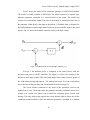
4.3 Doubly Fed Induction Generator Model in MATLAB
In MATLAB, the DFIG is represented using a phasor model. This model is
adapted to simulate the low frequency electromechanical oscillations over long
periods of time. In phasor simulation method, the sinusoidal voltages and currents are
replaced by phasor quantities at the system nominal frequency (60Hz). This model is
mostly used for transient stability studies of wind turbines. Shown in Fig.4.4 is the
model of the Double Fed Induction Generator used in MATLAB.
27
Texas Tech University, Santosh Pappu, August 2012
Fig.4.4 Model of the DFIG in MATLAB Simulink [11].
Fig.4.4 shows the inbuilt model of the DFIG in MATLAB Simulink. The
model as mentioned before is a phasor model. The generator is modeled as a constant
current source hence a resistor is placed in parallel to the generator. The parameters
used for the DFIG is listed below in Table 4.2.
28
Texas Tech University, Santosh Pappu, August 2012
Table 4.2: PARAMETERS OF DFIG
Parameter
Value
Nominal Power(MW)
1.5
Nominal Voltage(V)
575
Nominal Power Factor
0.9
Stator Resistance(pu)
0.0071
Stator Leakage Inductance(pu)
0.171
Rotor Resistance(pu)
0.005
Rotor Leakage Inductance(pu)
0.156
Magnetizing Inductance(pu)
2.9
Inertia Constant
5.0
Friction Factor
0.001
Pole Pairs
3
4.4 STATCOM
A static synchronous compensator (STATCOM), also known as a "static
synchronous condenser" ("STATCON"), is a regulating device used on alternating
current electricity transmission networks. It is based on a power electronics voltagesource converter and can act as either a source or sink of reactive AC power to an
electricity network. If connected to a source of power it can also provide active AC
power. It is a member of the FACTS family of devices.
Usually a STATCOM is installed to support electricity networks that have a
poor power factor and often poor voltage regulation. There are however, other uses,
the most common use is for voltage stability. A STATCOM is a voltage source
converter (VSC)-based device, with the voltage source behind a reactor. The voltage
source is created from a DC capacitor and therefore a STATCOM has very little active
power capability. However, its active power capability can be increased if a suitable
29
Texas Tech University, Santosh Pappu, August 2012
energy storage device is connected across the DC capacitor. The reactive power at the
terminals of the STATCOM depends on the amplitude of the voltage source. For
example, if the terminal voltage of the VSC is higher than the AC voltage at the point
of connection, the STATCOM generates reactive current; on the other hand, when the
amplitude of the voltage source is lower than the AC voltage, it absorbs reactive
power. The response time of a STATCOM is shorter than that of an SVC, mainly due
to the fast switching times provided by the IGBTs of the voltage source converter. The
STATCOM also provides better reactive power support at low AC voltages than an
SVC, since the reactive power from a STATCOM decreases linearly with the AC
voltage (as the current can be maintained at the rated value even down to low AC
voltage).
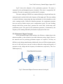
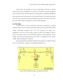
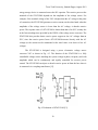
The STATCOM is designed using a power electronics voltage source
converter VSC as shown in Fig. 4.5. The function of the STATCOM is a fully
controllable voltage source matching the system voltage in phase, frequency and with
amplitude which can be continuously and rapidly controlled for reactive power
control. The STATCOM can inject or absorb reactive power to/from the bus where it
is connected via a coupling transformer [13].
Fig.4.5 Schematic of STATCOM [13].
30
Texas Tech University, Santosh Pappu, August 2012
The control system can be designed to maintain the magnitude of the bus
voltage constant by controlling the magnitude and phase shift of the VSC output
voltage. With the VSC voltage and the bus voltage, the output of the VSC can be
expressed as [10]:
(4.3)
(4.4)
Where P and Q are the active and reactive power of the STATCOM
respectively.
and
are the bus voltage and VSC voltage respectively. X is the
reactance of the coupling transformer and
voltages
and
is the phase difference between the
. If the AC voltage generated by the VSC is higher (lower) than the
system voltage , the STATCOM generates (absorbs) reactive power [8]. The
STATCOM is rated for 9.5MVA. It is operated in voltage regulation mode. The
voltage reference Vref is set at 1.0(pu). The STATCOM was set for a droop reactance
of 0.003(pu). The STATCOM provides reactive power for the wind farm as no fixed
capacitor banks are used for this configuration.
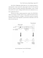
4.5 Topology of Wind Farms for Comparison of Wind Farms
The wind turbines are connected to produce 9MW of real power excluding
losses. The above mentioned models were used in MATLAB. Fig 4.6 shows the
topology of the wind turbines in the wind farm.
implemented for both the configurations.
31
The same topology has been
Texas Tech University, Santosh Pappu, August 2012
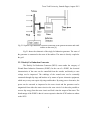
Fig 4.6 Topology of the wind turbines connected in a wind farm.
In Fig.4.6, the wind turbines are labeled from 1 to 18. Each turbine is
connected to a step up transformer which steps up the voltage to 25 kV from 575V.
This transformer is generally known as the padamount transformer and is fixed in the
hub of the turbine. The high side of the padamount transformer is connected to a cable
which extends up to roughly 1km. All the cables from the turbines route to the
substation which steps up the voltage to 120 kV and connect it via a transmission line
to the grid. The STATCOM is placed at the terminals of the wind farm to provide
reactive power support.
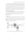
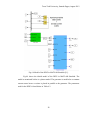
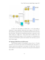
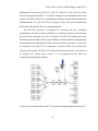
4.6 Topology of Wind Farms for HUB concept
Each wind farm comprises of the topology as shown in Fig. 4.6. The three
wind farms tap in from the same point on the transmission line. This point is a
collector system for the wind farms or also known as the Hub. Fig.4.7 shows the
model simulated. The wind farms are connected at the same point on the transmission
line at 345kV.
32
Texas Tech University, Santosh Pappu, August 2012
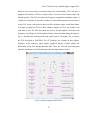
Fig.4.7 Schematic of wind farms for HUB concept.
Fig.4.7 shows the schematic of the interconnection of wind farms for Hub
concept. The three wind farms here share a common point of interconnection to the
grid. This common point of interconnection is termed as the Hub. A STATCOM is
connected to the wind farms for reactive power and voltage support during transient
conditions. The STATCOM can be disconnected from the wind farm by connecting
the STATCOM to a logic one. The wind farm is connected to a 25km transmission
line at 34.5kV. The voltage is then stepped up to 345kV and connected to a
transmission line of length 25km. At this point the three wind farms are interconnected
to form a Hub. This is then connected to the grid which is at 345kV.
33
Texas Tech University, Santosh Pappu, August 2012
CHAPTER 5
POWER QUALITY ANALYSIS USING PHASOR MEASUREMENT UNIT
This chapter focuses on research conducted on Power Quality Analysis at a
Semiconductor Fabrication Facility using a Phasor Measurement Unit (PMU). The
PMU used in this research is the SEL 421. The data collected using the PMU at the
facility was transmitted to the lab in Texas Tech via Ethernet. The data received was
processed by the SEL 3378 which is a data processor.
The purpose of this research was to analyze the quality of power coming into
the facility. The facility intends to install a wind turbine which will supply power to
the facility. Since the facility has sensitive equipment, any excursion in voltage,
frequency will cause damage to equipments in the facility. This could result in
millions of dollars loss. Recording the data of voltage, current and frequency coming
into the facility in the absence of a wind turbine can set standards of power quality
once the turbine is installed for power delivery to the facility.
The following sections describe the SEL 421, 3378 and the methodology
associated with data recording and associated software.
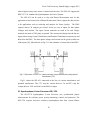
5.1 Power Quality Issues
Power Quality (PQ) related issues are of most concern nowadays. The
widespread use of electronic equipment, such as information technology equipment,
power electronics such as adjustable speed drives (ASD), programmable logic
controllers (PLC), energy-efficient lighting, led to a complete change of electric loads
nature. These loads are simultaneously the major causers and the major victims of
power quality problems. Due to their non-linearity, all these loads cause disturbances
in the voltage waveform [14].
Although many efforts have been taken by utilities, some consumers require a
level of PQ higher than the level provided by modern electric networks. This implies
that some measures must be taken in order to achieve higher levels of Power Quality.
The most common type of power quality issues are listed in the table below.
34
Texas Tech University, Santosh Pappu, August 2012
Table 5.1. Common Power Quality Issues [15]
Voltage sag (or dip)
Very short interruptions
Long interruptions
Voltage spike
Description: A decrease of the normal voltage level
between 10 and 90% of the nominal rms voltage at the
power frequency, for durations of 0,5 cycle to 1 minute.
Causes: Faults on the transmission or distribution
network (most of the times on parallel feeders). Faults in
consumer’s installation. Connection of heavy loads and
start-up of large motors.
Consequences: Malfunction of information technology
equipment, namely microprocessor-based control
Systems (PCs, PLCs, ASDs, etc) that may lead to a
process stoppage. Tripping of contactors and
electromechanical relays. Disconnection and loss of
efficiency in electric rotating machines.
Description: Total interruption of electrical supply for
duration from few milliseconds to one or two seconds.
Causes: Mainly due to the opening and automatic
reclosure of protection devices to decommission a faulty
section of the network. The main fault causes are
insulation failure, lightning and insulator flashover.
Consequences: Tripping of protection devices, loss of
information and malfunction of data processing
equipment. Stoppage of sensitive equipment, such as
ASDs, PCs, PLCs, if they’re not prepared to deal with
this situation.
Description: Total interruption of electrical supply for
duration greater than 1 to 2 seconds.
Causes: Equipment failure in the power system
network, storms and objects (trees, cars, etc) striking
lines or poles, fire, human error, bad coordination or
failure of protection devices.
Consequences: Stoppage of all equipment.
Description: Very fast variation of the voltage value for
durations from a several microseconds to few
milliseconds. These variations may reach thousands of
volts, even in low voltage.
Causes: Lightning, switching of lines or power factor
correction capacitors, disconnection of heavy loads.
Consequences: Destruction of components (particularly
electronic components) and of insulation materials, data
processing errors or data loss, electromagnetic
interference.
35
Texas Tech University, Santosh Pappu, August 2012
Table 5.1 Continued
Voltage swell
Description: Momentary increase of the voltage, at the
power frequency, outside the normal tolerances, with
duration of more than one cycle and typically less than a
few seconds.
Causes: Start/stop of heavy loads, badly dimensioned
power sources, badly regulated transformers (mainly
during off-peak hours).
Consequences:
Harmonic distortion
Description: Voltage or current waveforms assume
non-sinusoidal shape. The waveform corresponds to the
sum of different sine-waves with different magnitude
and phase, having frequencies that are multiples of
power-system frequency.
Causes: Classic sources: electric machines working
above the knee of the magnetization curve (magnetic
saturation), arc furnaces, welding machines, rectifiers,
and DC brush motors. Modern sources: all non-linear
loads, such as power electronics equipment including
ASDs, switched mode power supplies, data processing
equipment, high efficiency lighting.
Consequences: Increased probability in occurrence of
resonance, neutral overload in 3-phase systems,
overheating of all cables and equipment, loss of
efficiency in electric machines, electromagnetic
interference with communication systems, errors in
measures when using average reading meters, nuisance
tripping of thermal protections.
36
Texas Tech University, Santosh Pappu, August 2012
Table 5.1 Continued
Voltage
fluctuation
Description: Oscillation of voltage value, amplitude
modulated by a signal with frequency of 0 to 30 Hz.
Causes: Arc furnaces, frequent start/stop of electric
motors (for instance elevators), oscillating loads.
Consequences: Most consequences are common to
undervoltages. The most perceptible consequence is the
flickering of lighting and screens, giving the impression
of unsteadiness of visual perception.
Noise
Description: Superimposing of high frequency signals
on the waveform of the power-system frequency.
Causes: Electromagnetic interferences provoked by
Hertzian waves such as microwaves, television
diffusion, and radiation due to welding machines, arc
furnaces, and electronic equipment. Improper grounding
may also be a cause.
Consequences: Disturbances on sensitive electronic
equipment, usually not destructive.
Voltage Unbalance
Description: A voltage variation in a three-phase
system in which the three voltage magnitudes or the
phaseangle differences between them are not equal.
Causes: Large single-phase loads (induction furnaces,
traction loads), incorrect distribution of all single-phase
loads by the three phases of the system (this may be also
due to a fault).
Consequences: Unbalanced systems imply the
existence of a negative sequence that is harmful to all
three phase loads. The most affected loads are threephase induction machines.
5.2 SEL 421
The SEL-421 Relay is a high-speed transmission line protection relay featuring
single-pole and three-pole tripping and reclosing with synchronism check, circuit
breaker monitoring, circuit breaker failure protection, and series-compensated line
protection logic. The relay features extensive metering and data recording including
high-resolution data capture and reporting. Synchrophasor measurements are available
37
Texas Tech University, Santosh Pappu, August 2012
when a high-accuracy time source is connected to the relay. The SEL-421 supports the
IEEE C37.118, Standard for Synchrophasors for Power Systems.
The SEL-421 can be used as a relay and Phasor Measurement unit. In this
application it has been used as a Phasor Measurement Unit to capture the data and use
it for applications such as archiving and analysis for Power Quality. The PMU
captures data at 30 samples per second. It has two sets of inputs for three phase
Voltages and currents. The input Current terminals are rated at 5A and Voltage
terminals are rated at 120V phase to ground. The current and voltage from the line are
stepped down using Current Transformers and Potential Transformers respectively and
then fed to the PMU. The three phase voltages and currents can be given to either one
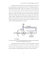
of the inputs [16]. Shown below in Fig.5.1 is the schematic of connection of the PMU.
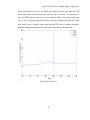
Fig.5.1 Schematic of SEL-421 connected using current transformers and potential
transformers [16].
Fig.5.1 shows the SEL-421 connected to the line via current transformers and
potential transformers. The CT’s step the current down to 5A and PT’s step the
voltage down to 120V and feed it to the PMU as inputs.
5.3 Synchrophasor Vector Processor-SEL 3378
The SEL-3378 Synchrophasor Vector Processor uses synchronized phasor
measurements for real-time power system monitoring, control, and protection. The
SEL-3378 acquires and time correlates synchrophasor data from various Phasor
38
Texas Tech University, Santosh Pappu, August 2012
Measurement Units such as SEL-351, SEL-421, SEL-451 relays, and from other
devices that support the IEEE C37.118-2005, Standard for Synchrophasors for Power
Systems. The SEL-3378 receives synchrophasor messages through serial and Ethernet
communications [17]. The SEL-3378 was setup in Texas Tech and communication
between the PMU and the Processor through Ethernet.
The SEL-3378 provides a mechanism for collecting and time correlating
synchrophasor data from as many as 20PMUs at a maximum data rate of 60 messages
per second with a message size of up to 354 bytes. The SEL-3378 includes the Power
Calculation Function Block, Phase Angle Difference Function Block, Modal Analysis
Function Block and Substation and State Topology Processor Function. A GPS clock
is connected to the SEL-3378 to synchronize it with the PMUs for real-time data
collection and analysis. The SEL-3378 allows the data from the PMU to be archived
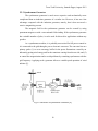
for analysis [16]. Shown below in Fig 5.2 is an application of the SEL-3378
communicating through the Ethernet.
Fig.5.2 System Configuration of SEL-3378 communicating through the Ethernet [17].
39
Texas Tech University, Santosh Pappu, August 2012
The connection to the computer can be through serial port or Ethernet. Here the
PMUs and other Phasor Data Concentrators send data to the SEL-3378 through
Ethernet. The SEL-3378 processes the data from the PMUs and sends it to the
computer for applications such as archiving and real-time data plots.
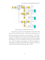
5.4 SVP Configurator
The SVP Configurator allows you to build projects based on your required
applications. The Run Time System (RTS) turns the SEL-3378 into an IEC 61131-3
programmable logic controller (PLC). The programming languages that the SVP
Configurator offers conform to the requirements of IEC 61131-3, an international
standard for programming languages of PLCs [17]. The code for initialization of the
processor was written in the SVP Congfigurator. The SVP Configurator supports all
the languages that the IEC 61131-3 standard describes. These languages can be
characterized as textual and graphical languages.
The SVP Configurator code involves creating project files for Time Alignment
Client Server (TCS) that provides time-aligned IEEE C37. 118-2005, Standard for
Synchrophasors for Power Systems, synchrophasor messages to internal and external
clients and provides an interface for transmitting control commands. The Configurator
also involves providing an interface for accessing PMCU data for user applications,
Power Calculation which calculates real and reactive power based on user assigned
phasors, Phase angle Difference Monitor, Modal Analysis and Substation and
Topology Processor. For this project involving Power Quality Analysis, the Time
Alignment Client Server, Power Calculation and Phasor Measurement and control
Unit Input interfaces were used.
The code in the Time Alignment Client Server includes the IDCODE for the
PMU, type of connection, status, and transport scheme, IP address of the Processer,
PMU and the computer where the data archived would be stored. Each PMU has a
unique IDCODE provided by the manufacturer. The connection between the Processor
and PMU can be serial communication or as in this case Ethernet. The data ports and
40
Texas Tech University, Santosh Pappu, August 2012
command ports of the Processor are given different port numbers to avoid conflict.
The Processor allows four different transportation schemes for data which can be
UDP, UDP_T, UDP_F and TCP. The Message rate of the PMU was set at 30 samples
per second. When the PMU is stationed in a different network than that of the
Processor, it is necessary to make sure that the subnet and the gateway of the devices
entered are correct. The subnet mask and the gateway are important parameters when
both the equipments are not on the same device [17].
The Power Calculation block calculates the real and reactive power based on
user-selected voltage and current phasors. PWRC outputs the instantaneous values of
the real power (kW) and reactive power (kVAR) with their corresponding timestamps.
The equations below show the implementation of the function block [17].
P= (RE_V*RE_I+IM_V*IM_I)/1000
Q= (IM_V*RE_I-RE_V*IM_I)/1000
(5.1)
(5.2)
The Real Power P is in kW and Reactive Power Q is in kVAR. In the above
equations IM stands for imaginary and RE stands for real.
5.5 SEL SynchroWave Archiver
The SEL-5076 SynchroWave Archiver Software provides continuous or triggered
storage of power system data. Data can be archived over a wide geographic area by
using the accurate time stamps. The archiver was set up to record the data from the
PMU connected at the Facility. The archiver receives data from the Processor which in
turn receives data from the PMU. The archiver plots the values of the voltages,
currents of the inputs along with frequency, delta frequency, real and reactive power in
each individual phase and also the total three phase power. It samples data at the rate
of 30 samples per second.
The data archived is stored in the form of CSV or
Comtrade [18]. The Main Menu of the archiver consists of a GUI for means to add or
remove PMUs, to modify the archiver configuration and communication. A new
source or PMU can be added by clicking on New Source and by adding the IDCODE
of the corresponding PMU. The data to be archived can be chosen to be stored in a
41
Texas Tech University, Santosh Pappu, August 2012
specific location as specified by the user. The communication for the PMU should be
setup by mentioning the IP address of the PMU and scheme of transportation of data.
The data recording will start once Activate Archiver is selected. The data will be
stored in the selected folder. The archiver will record the data points of the parameters
selected. Since only one input was connected each on the current and voltage
terminals, the number of parameters that were recorded was seventeen which included
frequency and delta frequency. Continuous data storage mode was used for this
project to collect large data for analysis of Power Quality.
5.6 SEL SyncrhoWave Console
The SynchroWave Console is wide area visualization software for synchrophasors
that offers flexibility for operators and engineers to view multiple displays in multiple
dockable windows and customize the visualizations to optimize the ability to monitor
the power system. The Console displays a graphical interpretation of real time data. It
can plot magnitudes of phase voltages and currents, phase angles of the three phases,
frequency and delta frequency. To connect the Console to the PMU concerned, the
communication parameters such as IP address and transportation scheme need to set
up. Here the IP address refers to the IP address of the Processor as the PMU sends data
to the Processors which in turn process the data from the PMU [18].
Once the communication parameters are set up, the Console can connect to the
Processor and the real time data can be seen on the screen of the console. The data by
default is recorded for duration of five minutes. This duration can be changed to a
maximum of twenty four hours. Shown in Fig.5.3 is a plot of Current in Phase C. This
data has been recorded for duration of one hour. The data is being recorded from the
PMU located at the Semiconductor Foundry Fabrication Facility. The plot included
some interruption which was due to loss of communication between the Processor and
PMU.
42
Texas Tech University, Santosh Pappu, August 2012
Fig.5.3 Plot from the SynchroWave Console of the Current in Phase C.
5.7 Point of Connection of the PMU
The point of connection of the PMU in the Facility is shown below in Fig. 5.4.
The voltage was stepped down to 120V using a potential transformer and connected to
the PMU.
43
Texas Tech University, Santosh Pappu, August 2012
Fig. 5.4 A part of the line diagram which shows the point of connection of the PMU.
5.8 Baseline of Parameters of Power Flowing into the Facility
It is important to establish a baseline for the values of the parameters such as
voltage and frequency coming into the Facility from the utility. Establishing and
knowing this baseline for the power quality is imperative when deciding which form
of green energy to choose, or which manufacture to negotiate with. When
understanding this, the wind turbine manufactures that are providing and installing the
turbines have to guarantee a power quality that will match the current utility power.
Shown in Table.5.1, are the variations of the parameters of the data that was recorded
from the PMU at the Facility.
TABLE 5.1
VARIATION OF PARAMETERS OF THE DATA RECORDED
Parameters
Nominal Voltage
Variation (max)
Voltage ( Va, Vb, Vc)
120 V
0.6V
44
Texas Tech University, Santosh Pappu, August 2012
Frequency
60Hz
0.2Hz
The voltage on all three phases varied a maximum of 0.6V from the nominal
value. The frequency varied a maximum of 0.2Hz from its nominal voltage.
5.9 Description of Code for Power Quality Analysis
The data that the PMU samples and saves it’s information on are: all three
voltage and current phases, with their respective real and imaginary parts, power
factor, frequency, the change in frequency, and the real, imaginary, and magnitude
parts of the power. The PMU saves millions of data points into thousands of excel
files. For this data mining to be useful, a program needs to be implemented to
systematically analyze this raw information, and present it in a clear, concise, and
accurate format for a person to comprehend.
The PMU samples the data 30 times per second, or 1800 times per minute.
This data is saved in the form of excel files in a specific directory. Each excel file
contains the information for two minutes of wind turbine function. Due to issues such
as transients, it is necessary to check the data coming from PMU to see whether they
meet the standard criteria or not. Any sudden spike or inconsistency can seriously
damage electronic devices. In order to do this, a MATLAB program was developed.
This MATLAB program checks the input frequency, and three-phase voltage. It takes
an average of two seconds for the code to process one excel file containing two
minutes of data. Fig. 4.5 describes the working of the code in the form of a flowchart.
45
Texas Tech University, Santosh Pappu, August 2012
Fig.5.5 Flowchart description of the code.
In order to observe and analyze any interruption, or possible error, input
frequency, and voltages for all phases are checked through the code. An upper bound
and lower bound can be set for each variable. These values are usually 3 Hz from 60
Hz for frequency, and 5 V from 120V for each phase in the three-phase voltage.


46
Texas Tech University, Santosh Pappu, August 2012
However users can set their own desired values for each boundary. The Code uses a
graphical user interface (GUI) to set these values. User can set the desired values, and
start the analysis. The GUI also shows the frequency, magnitudes, and phase angles of
voltages for each phase in real time. Number of errors and disruptions are also shown
on the GUI. As the code processes the excel files, the phase angles for all three phases
of voltage is graphed on GUI, to show whether voltages are 120 out of phase with
each other or not. The GUI also shows the lowest, and the highest values that each
frequency, and voltages in all three phases that have been recorded during the analysis.
Fig. 4.5 describes the working of the code in the form of a flowchart. Fig. 4.6 shows
the GUI developed in MATLAB. The GUI displays the voltages in three phases,
frequency, delta frequency, phase angles, graphical display of phase angles and
information of the files having abnormal data. The code will start processing data
when the start button is clicked and stops when the stop button is clicked.
Fig.5.6 GUI developed in MATLAB.
47
Texas Tech University, Santosh Pappu, August 2012
CHAPTER 6
RESULTS FOR COMPARATIVE STUDY OF WIND TURBINES
The analysis was carried out on MATLAB-Simulink simulation environment.
Both the configurations were simulated for the same length of time to make the
analysis comparable. The same base values were used for both the configurations. The
configurations were simulated for various wind conditions and fault conditions to
check parameters like reactive power consumption, voltage stability, and active power
transmission. The various conditions for both wind farms are simulated and
demonstrated below. The voltage values are displayed in pu system and reactive
power and active power are displayed in MW and MVAR respectively. The
measurements are recorded at the terminals of the wind farm and at the 25kV bus for
both the wind farms.
6.1 Wind Speeds ranging from 3-6m/s
Both the configurations have been simulated for wind speeds ranging from 3-6m/s
as shown in Fig. 4.1. The step change causes a change in reactive power and active
power. Fig.6.1 shows the reactive power consumed for both the topologies. The wind
farm consisting of DFIG consumes reactive power from 40sec. This is because the
DFIG transmits power at low wind speeds. As the wind speed steps up to 6m/s, the
DFIG starts generating active power and hence consuming reactive power, while the
wind farm consisting of FSIG does not consume any reactive power as it does not
generate any active power at low wind speeds. The voltage on the 25kV bus is stable
for both the configurations as consumption of reactive power consumption is very less
for low wind speeds. Fig.6.2 shows the active power transmission to the grid of both
wind farms for this particular wind profile. The first few seconds show the initial
transients on both the configurations. The wind farm consisting of FSIG does not
generate any power for both the wind speeds. The wind farm consisting of DFIG starts
generating active power as the wind speed steps at 20sec.
48
Texas Tech University, Santosh Pappu, August 2012
Fig.6.1 Reactive power consumption for both wind farms for wind speeds ranging
from 3-6m/s.
49
Texas Tech University, Santosh Pappu, August 2012
Fig 6.2 Active Power transmission for wind speeds ranging from 3-6m/s.
6.2 Wind speeds ranging from 9-12m/s
The wind farms were then simulated for wind speeds ranging from 9-12m/s. The
wind speed 12m/s is the rated wind speed for both wind farm configurations. Fig 6.3
shows the reactive power consumption of both wind farms. The reactive power
consumption rises as the wind speed steps up from 9m/s to 12m/s due to increase in
generation of active power up to rated capacity. The response of the wind farm with
FSIG is immediate whereas the consumption of reactive power attains steady state
after a few seconds for the wind farm with DFIG. Fig.6.4 shows the voltage at the
25kV bus for both wind farms. The voltage at the bus rapidly reduces for wind farm
consisting of FSIG as the wind speed increases from 9m/s to 12m/s due to increase in
50
Texas Tech University, Santosh Pappu, August 2012
reactive power consumption. It gradually decreases for the DFIG wind farm. Fig.6.5
shows the active power generation of both wind farms for this wind profile. Both wind
farms reach rated capacity of generation when the wind speed is stepped up to 12m/s.
As shown in Fig.6.5, the wind farm with FSIG responds faster than wind farm with
DFIG thereby capturing more power for longer than the configuration with DFIG.
Fig.6.3 Reactive Power consumption for both wind farms.
51
Texas Tech University, Santosh Pappu, August 2012
Fig.6.4 Voltage at 25kV bus for both wind farms.
Fig.6.5 Active Power transmitted from both wind farms.
52
Texas Tech University, Santosh Pappu, August 2012
6.3 Wind Speeds ranging from 21-24m/s
The wind farms were then simulated for wind speeds ranging from 21-24m/s
nearing cutoff wind speed. Fig.6.6 shows the reactive power consumed for both wind
farms. The initial few seconds are the startup transients as the turbine starts rotating
for a wind speed of 21m/s. The wind farm with FSIG trips after 5sec due to over speed
and does not consume any reactive power after that. The DFIG trips due to over speed
when the wind speed is stepped up to 24m/s and consumes reactive power until then.
Fig.6.7 shows the voltage at the 25kV bus. Due to the initial wind speed of 21m/s,
transients are present due to high reactive power consumption at that wind speed and
settles once the turbine is tripped due to over speed in FSIG wind farm. The voltage
dips down to a certain value due to consumption of reactive power. Once the turbine
trips due to over speed, the voltage level increases to 1pu. Fig.6.8 shows active power
generated from the two wind farms. The DFIG generates active power till the wind
speed reaches 24m/s. The relay trips the generator due to over speed condition. The
wind farm consisting of FSIG does not generate any power for both wind speeds. The
first few seconds display the initial transients of the wind farm experienced at startup
due to the high wind speed.
53
Texas Tech University, Santosh Pappu, August 2012
Fig.6.6 Reactive Power consumed for both wind farms.
Fig.6.7 Voltage at 25kV bus for both wind farms.
54
Texas Tech University, Santosh Pappu, August 2012
Fig.6.8 Active Power generated for wind speeds from 21-24m/s
6.4 Equal Power Lost
Equal amount of power was taken out from the two configurations to check the
active power transmitted, reactive power consumed and the voltage at the bus at point
of common coupling. A three phase fault was installed on three turbines in the wind
farm with 500kW and on one turbine in the wind farm consisting of 1.5MW DFIG
turbines. The wind farm is simulated for wind speeds from 9-12m/s which steps up
from 9m/s to 12m/s at 20sec.A fault lasting for 0.1sec occurring on the terminals of
the wind turbine was simulated on both the wind farms. Fig.5.9 shows the reactive
power consumption for this scenario. The reactive power consumed is less for DFIG
as shown. The DFIG takes more reactive VARs during the fault and settles down after
the fault. The DFIG takes longer time to reach steady state than the FSIG which also
consumes more VARs than the DFIG during steady state. Fig.6.10 shows the active
55
Texas Tech University, Santosh Pappu, August 2012
power transmitted to the grid. The DFIG takes power from the grid when the fault
occurs and returns to generating mode once the fault is cleared. For speeds up to
9m/s, the DFIG generates more active power than the FSIG. As the wind speed steps
up to 12m/s, the power generated increases on both configurations. But the DFIG
takes longer time to achieve steady state than the FSIG due to machine dynamics.
Both the configurations generate the same power once they reach steady state.
Fig.6.9 Reactive power consumption when a three phase to ground fault occurs at
40sec to last for 0.1sec.
56
Texas Tech University, Santosh Pappu, August 2012
Fig.6.10 Active Power transmitted when 1.5MW is lost in both wind farms.
6.5 Equal Number of turbines Lost to Faults
Situations in which three phase to ground faults were installed on the terminals
of equal number of turbines on both the wind farm configurations. Three phases to
ground faults were installed on two wind turbines in each configuration. In the wind
farm consisting of the DFIG, two additional turbines were tripped due to faults on two
other turbines. The reason for this trip was AC under voltage. The voltages on both the
turbines were less than 0.75pu for more than 5sec. The fault on both the turbines
caused high transient currents due to which the DC voltage increased beyond 1900V
which caused the relay to trip both the turbines. The reactive power consumed by the
DFIG is less than that consumed by the FSIG. The difference being in the order of
1MVAR. Fig.6.11 shows the active power transmitted in both cases. For the wind
57
Texas Tech University, Santosh Pappu, August 2012
farm consisting of the DFIG, the active power generated is 2.5MW as four turbines are
totally tripped. Whereas in the wind farm consisting of FSIG, only two turbines are
lost to faults and a total of 7.2MW real power is transmitted to the grid. This way the
FSIG generates more active power than the DFIG due to three phase faults on two
turbines. Fig.6.12 shows the Electrical Torque of DFIG and FSIG. A three phase to
ground fault is installed at 40sec. The torque increases gradually and then settles down
at zero after the fault has occurred.
Fig.6.11 Active Power transmitted to the grid from both the wind farms.
58
Texas Tech University, Santosh Pappu, August 2012
Fig.6.12 Electrical Torque of both the generators when a three phase fault occurs.
59
Texas Tech University, Santosh Pappu, August 2012
CHAPTER 7
RESULTS FOR EVALUATION OF HUB CONCEPT
The simulation was carried out in MATLAB-Simulink simulation
environment. The simulation time was 50secs. The model was simulated for a constant
wind speed of 12m/s to attain steady state fast. The model has been simulated for
various transient conditions. The voltage and torque values are recorded in pu system.
The active power and reactive power values are recorded in MW and MVAR
respectively. The measurements are recorded at the 34.5kV bus for the wind farms and
345kV bus at the point of interconnection. This section demonstrates the working of
the model for rated conditions and for faults at various locations.
7.1 Rated Conditions
The wind farms are simulated for rated conditions. A wind speed of 12m/s
is given as input to the wind turbines in all three wind farms. The active power,
voltage and reactive power at the point of interconnection are recorded. The active
power at this point is the total power generated from all three wind farms including
transmission losses. The wind turbines are set to generate 0.95pu of the mechanical
power at this wind speed. Fig.7.1 shows the active power recorded at the 345kV bus.
This power is the total power generated by all the three wind farms. The output
reaches steady state after certain time. The time taken is due to start up transients. The
power recorded at the point of interconnection is about 25MW. The three wind farms
are rated for 27MW.
60
Texas Tech University, Santosh Pappu, August 2012
Fig.7.1 Active Power at the point of Interconnection
7.2 Fault on One Wind Turbine in Wind Farm
A three phase to ground fault was installed on one wind turbine in wind
farm A. The response of the wind turbines in wind farm A and B to the fault were
recorded. The fault was installed to trigger at time 35sec for duration of 0.1sec. When
the fault acts on the wind turbine, the voltage of the wind turbine reduces to 0.1pu.
The relay senses the dip in voltage and trips the wind turbine. The effect of this fault
on the wind turbine in the neighboring wind farm is analyzed. Fig.7.2 Shows the
voltage at the turbine which has been shorted in wind farm A.
61
Texas Tech University, Santosh Pappu, August 2012
Fig.7.2 Voltage at the terminals of the wind turbine with three phase to ground fault
Fig.7.3 shows that the fault on wind turbine in wind farm A has an effect on
the wind farm B. This is due to the fact that during the fault, the wind turbine in wind
farm A absorbs excessive reactive power from the grid to support the voltage.
This causes a dip in the voltage of wind farm B due to absorption of reactive
power by the turbine subject to fault in wind farm A.
62
Texas Tech University, Santosh Pappu, August 2012
Fig.7.3 Voltage at terminals of wind farm B.
Fig.7.4 shows the electrical torque of a wind turbine in the wind farm B. When
the fault occurs at 35sec in Wind Farm A, pulsations occur in the rotor of the wind
turbine in wind farm B and cause pulsations in the electrical torque.
63
Texas Tech University, Santosh Pappu, August 2012
Fig.7.4 Electrical Torque of wind turbine in wind farm B.
7.3 Fault on Wind Farm A
A three phase to ground fault was installed on the terminals of the wind farm
A. The response of the neighboring wind farms to the fault was analyzed. The voltage
at the terminals of the wind farm B was analyzed for impact of the fault on the
neighboring wind farm. Fig.7.5 shows the voltage at wind farm A. At 35sec, a three
phase to ground fault is installed. The fault lasts for 0.1sec.
64
Texas Tech University, Santosh Pappu, August 2012
Fig.7.5 Terminal Voltage of Wind farm A.
Fig.7.5 shows the voltage at the terminals of the wind farm B. At 35sec, the
voltage reduces by 0.2pu for about 0.1 sec. This implies that a fault on the wind farm
A causes an impact on the voltage and reactive power of wind B and C. This is due the
excessive reactive power drawn from the grid by wind farm A to support the voltage
dip. This excessive consumption of reactive power from the grid causes dip in the
reactive power consumed by wind farm B and causes a reduction in the voltage.
65
Texas Tech University, Santosh Pappu, August 2012
CHAPTER 8
RESULTS FOR POWER QUALITY ANALYSIS USING A PMU
The data recorded from the PMU set up at the semiconductor facility was
archived. A code developed in MATLAB reads the excel files from the specific
directory that was set by the user, and PMU is saving the data into. Frequency and
three-phase Voltage are compared to the boundaries set by the user. In case of sudden
jump (if the magnitude of any phase in the input 3-phase voltage, or the frequency is
out of range), code will consider the error, and alert the user. Code will plot three
graphs to provide enough information for analyzing the error. Fig.8.1 displays the GUI
when a excursion is found in the values of the excel sheet given as input. It shows the
frequency, delta frequency and voltage in all three phases which contain data which is
not within the limits.
Fig.8.1 GUI display when there is an excursion in the parameters.
66
Texas Tech University, Santosh Pappu, August 2012
This information contains the plots of three phases of voltage, frequency, and
delta frequency vs. time. All these graphs are plotted for the range of two minutes
before the incident, and two minutes after it (three excel files on average). These
graphs will be saved to respective sub-folders. Each sub-folder is named after the
number of error, and is under the folder, which determines the type of error that has
occurred. For example, if the voltage in phase A goes out of range for the first time, a
sub-folder with the name of 1 is created under the folder with the name of
“VoltagePhaseAError”. Fig.8.2 shows the folder where the excel sheets which contain
any excursion in data are saved.
Fig.8.2 Folder where the erroneous files are saved.
Each sub-folder also includes the excel file that contains the error. All these
folders are saved in the directory determined by the user. Code will continue analyzing
the data for all the excel files. Fig.8.3 shows the subfolder containing the waveforms
of the parameters and the excel sheet containing data.
67
Texas Tech University, Santosh Pappu, August 2012
Fig.8.3 Sub folder where the waveforms and excel sheet containing the data are saved.
68
Texas Tech University, Santosh Pappu, August 2012
CHAPTER 9
CONCLUSION
The transient models of FSIG and DFIG were developed and simulated in
MATLAB- Simulink. It is becoming increasingly important to decide which topology
of wind farm should be implemented when starting a wind farm. This model is
simulated for all wind conditions to demonstrate the response of the two topologies to
all wind conditions and fault conditions and show the reactive power consumed,
voltage stability at the point of common coupling and active power transmitted to the
grid during all wind conditions. At cut in, rated and cut off wind speeds the DFIG is
superior than FSIG in the terms of active power transmitted, voltage stability. The
reactive power consumed also is less than the FSIG. The performance of both the
topologies is same when equal amount of power was taken out due to faults. Hence all
the above factors should be considered while deciding which topology of wind farms
would be used for generation of wind energy.
The Hub concept was discussed and modeled on the same lines in MATLABSimulink. A transient analysis was conducted on the wind farm in different scenarios.
It was concluded that the installations of faults in one wind turbine caused an impact
on the neighboring wind farms. This is due to excessive reactive power consumption
from the grid for voltage support.
The installation of FACTS devices such as
STATCOM reduces the impact of the fault on neighboring wind farms.
A unique method for analyzing Power Quality was developed in MATLAB. A
set of limits was established for parameters such as voltage and frequency for data
analysis of Power Quality. The power coming from the utility had no aberrations from
the normal as expected. The data analyzed before the installation of the wind turbine at
the Facility forms an important basis for analysis after the installation of the wind
turbine. After the installation of the turbine, continuous data monitoring would be
taking place with the help of the PMU. The PMUs should be placed at various critical
locations for monitoring of Power Quality from the Wind Turbine. The data collected
69
Texas Tech University, Santosh Pappu, August 2012
would be analyzed using the code developed. This would help maintain good Power
Quality at the Facility.
70
Texas Tech University, Santosh Pappu, August 2012
CHAPTER 10
FUTURE WORK
The models built for comparison of wind farms for different ratings and
evaluation of hub concept will be validated by simulating the models in software such
as PSSE/ PSLF. The code built for evaluating power quality will be made to evaluate
more data like THD, voltage sags, dips, swells. The PMU will be installed once the
wind turbine at XFAB has been installed and data will be recorded and evaluated.
71
Texas Tech University, Santosh Pappu, August 2012
REFERENCES
[1] Thomas Ackerman, “Wind Power in Power Systems,” Royal Institute of
Technology, Stockholm, Sweden.
[2] http://en.wikipedia.org/wiki/Wind_turbine
[3] http://planet-energy.org/sustainable_energy/Blog_17_page.html
[4] AGCTF 9/1/11 Meeting Materials.
[5] http://en.wikipedia.org/wiki/Power_quality
[6] “Mathworks documentation”. Available: http://www.mathworks.com.
[7] http://www.ncl.ac.uk/eee/research/project/974
[8] http://www.almohandes.org/vb/showthread.php?t=47664
[9] http://www.donsion.org/calidad/cc8/c8-11.pdf
[10] AGCTF 9/6/11 Whitepaper,
[11] Kenneth E. Okedu, “Transient Analysis of DFIG and IG during Grid Fault”, in
The Pacific Journal of Science and Technology.
[12] “MATLAB/Simulink Documentation”. Available: http://www.mathworks.com.
[13] V.Ramakrishnan and S. K. Srivatsa. “Pitch Control of Wind Turbine Generator
by using New Mechanism”.
[14] Omar Noureldeen, “Low Voltage Ride through Strategies for SCIG Wind
Turbines Interconnected Grid”, in International Journal of Electrical & Computer
Sciences IJECS-IJENS Vol: 11 No: 02.
[15] A.de Almeida, L. Moreira, J.Delgado, “Power Quality Problems and New
Solutions”.
[16] “Power Quality Problems and New Solutions “ A. de Almeida, L. Moreira. J.
Delgado
[17] SEL-421 Relay Protection and Automation System Instruction Manual,
Schweitzer Engineering Laboratories, INC.
[18] SEL-3378 Synchrophasor Vector Processor Instruction Manual, Schweitzer
Engineering Laboratories, INC.
[19] SEL-5078 SynchroWave console User Manual, Schweitzer Engineering
Laboratories, INC.
72
Texas Tech University, Santosh Pappu, August 2012
[20] SEL-5076 SynchroWave Archiver User Manual, Schweitzer Engineering
Laboratories, INC.
73
Texas Tech University, Santosh Pappu, August 2012
PUBLICATIONS
1. Santosh Pappu and Stephen Bayne, “Evaluation of Hub Concept for Wind
Turbines”, IEEE Power and Energy Conference at Illinois 2012.
2. Santosh R Pappu, Arash Rahnama, Mathew Tovar, Stephen Bayne, Boby Little,
Sid Friend and Marcus Borhani, “ Power Quality Analysis at a Sensitive Load using a
Phasor Measurement Unit”, IEEE Green Technologies Conference 2012.
3. Santosh Pappu, Sandeep Nimmagadda and Stephen Bayne, “Analysis and
Comparison between two wind farms consisting of 500kW midsize turbines and
1.5MW turbines.”, IEEE Power Electronics and Machines in Wind Applications –
PEMWA 2012 (accepted-to be presented on July 17th, 2012).
74