Download Visualization of Tool overlapping Dependencies in a Traceability

Visualization of Tool overlapping
Dependencies in a Traceability
Framework
Leon Bornemann
Institut für Informatik
Freie Universität Berlin
A thesis submitted for the degree of
Bachelor of Science
Acknowledgements
First of all I would like to thank Prof. Dr. Ina Schieferdecker for
supervising this thesis and thus enabling me to write my bachelor thesis about the fascinating topic of traceability. Furthermore I would
like to thank Jürgen Großmann and Michael Berger from the Fraunhofer FOKUS institute for their continous support during this thesis.
My exceptional gratitude goes to my friends Carsten Flöth and KaiFabius Pribyl for proofreading this thesis. Lastly I would like to thank
my parents for their everlasting encouragement and support in every
phase of my life.
Abstract
In the developing process of a technical system a large number of artifacts is created. In order to manage the dependencies between different artifacts created by different tools, the tool overlapping traceability framework RiskTest has been developed. RiskTest administers the
artifacts and their dependencies as a graph. While it is already possible to connect different artifacts via RiskTest, the resulting graph
needs to be visualized properly to allow the user to easily identify
traces throughout the whole project. The visualization needs to provide an efficient way for the user to gain insight into a complex graph
structure. In this bachelor thesis the necessary requirements for such a
visualization are analyzed, different approaches for dealing with graph
visualization are evaluated, different frameworks and tools are closer
looked upon, their usefulness for these particular requirements is assessed and finally a fitting visualization is implemented and added to
the RiskTest traceability framework.
Contents
Contents
iii
List of Figures
vi
1 Introduction
1
2 State of the Art: Traceability Tools and Graph Drawing Algorithms
2.1 Traceability . . . . . . . . . . . . . . . . . . . . . . . . . . . . . .
2.1.1 Traceability in General . . . . . . . . . . . . . . . . . . . .
2.1.2 Traceability in Different Domains . . . . . . . . . . . . . .
2.2 Graph Drawing . . . . . . . . . . . . . . . . . . . . . . . . . . . .
2.2.1 Layout Evaluation . . . . . . . . . . . . . . . . . . . . . .
2.2.1.1 Edge Crossings . . . . . . . . . . . . . . . . . . .
2.2.1.2 Edge Bends . . . . . . . . . . . . . . . . . . . . .
2.2.1.3 Local Symmetry . . . . . . . . . . . . . . . . . .
2.2.1.4 Edge length . . . . . . . . . . . . . . . . . . . . .
2.2.1.5 Vertex Distribution . . . . . . . . . . . . . . . . .
2.2.2 Graph Drawing Algorithms . . . . . . . . . . . . . . . . .
2.2.2.1 Planar Graph Drawing Algorithms . . . . . . . .
2.2.2.2 Symmetric Graph Drawing Algorithms . . . . . .
2.2.2.3 Hierarchical Graph Drawing Algorithms . . . . .
2.2.2.4 Tree Drawing Algorithms . . . . . . . . . . . . .
2.2.2.5 Spine and Radial Graph Drawing Algorithms . .
2.2.2.6 Circular Graph Drawing Algorithms . . . . . . .
iii
4
4
4
5
6
6
6
7
7
7
8
8
9
9
10
10
10
10
CONTENTS
2.2.2.7
2.2.2.8
2.2.2.9
Simultaneous Graph Drawing Algorithms . . . .
Force-Directed Graph Drawing Algorithms . . . .
Three-Dimensional Graph Drawing Algorithms .
3 Analysis
3.1 The RiskTest Traceability Framework . .
3.1.1 Current State of RiskTest . . . .
3.1.2 Software Architecture of RiskTest
3.2 Requirements Collection . . . . . . . . .
3.2.1 Data and Appearance . . . . . .
3.2.2 Interaction . . . . . . . . . . . . .
3.2.3 Hierarchies . . . . . . . . . . . .
3.2.4 Filtering . . . . . . . . . . . . . .
3.2.5 Summary . . . . . . . . . . . . .
3.3 Graph Drawing Tools and Frameworks .
3.3.1 Tool: yEd Graph Editor . . . . .
3.3.2 Framework: yFiles . . . . . . . .
3.3.3 Framework: JUNG . . . . . . . .
3.3.4 Framework: OGDF . . . . . . . .
3.3.5 Overall Comparison and Decision
3.4 Graph Drawing Algorithms . . . . . . .
11
11
11
.
.
.
.
.
.
.
.
.
.
.
.
.
.
.
.
12
12
12
15
16
17
19
20
23
24
25
25
25
26
27
28
30
4 Design
4.1 Design of the Visualization . . . . . . . . . . . . . . . . . . . . . .
4.2 Design of the Software Architecture . . . . . . . . . . . . . . . . .
34
34
35
5 Implementation
5.1 Resulting User Interface . . . . . . . . . . . . . . .
5.2 Packages . . . . . . . . . . . . . . . . . . . . . . . .
5.3 Usage of the JUNG Framework . . . . . . . . . . .
5.4 Important Classes and Interactions Between Them
5.4.1 Realization of the MVP Pattern . . . . . . .
5.4.2 Bridge to the RiskTest Plugin . . . . . . . .
5.4.3 Visualization of the Views . . . . . . . . . .
38
38
41
42
43
43
44
44
iv
.
.
.
.
.
.
.
.
.
.
.
.
.
.
.
.
.
.
.
.
.
.
.
.
.
.
.
.
.
.
.
.
.
.
.
.
.
.
.
.
.
.
.
.
.
.
.
.
.
.
.
.
.
.
.
.
.
.
.
.
.
.
.
.
.
.
.
.
.
.
.
.
.
.
.
.
.
.
.
.
.
.
.
.
.
.
.
.
.
.
.
.
.
.
.
.
.
.
.
.
.
.
.
.
.
.
.
.
.
.
.
.
.
.
.
.
.
.
.
.
.
.
.
.
.
.
.
.
.
.
.
.
.
.
.
.
.
.
.
.
.
.
.
.
.
.
.
.
.
.
.
.
.
.
.
.
.
.
.
.
.
.
.
.
.
.
.
.
.
.
.
.
.
.
.
.
.
.
.
.
.
.
.
.
.
.
.
.
.
.
.
.
.
.
.
.
.
.
.
.
.
.
.
.
.
.
.
.
.
.
.
.
.
.
.
.
.
.
.
.
.
.
.
.
.
.
.
.
.
.
.
.
.
.
.
.
.
.
.
.
.
.
.
.
.
.
.
.
.
.
.
.
.
.
.
.
.
.
.
.
.
.
.
.
CONTENTS
5.5
Graph
5.5.1
5.5.2
5.5.3
Layout Algorithms . . . . . . . . .
Fruchtermann-Reingold Algorithm
Sugiyama Method . . . . . . . . . .
Circle Layout . . . . . . . . . . . .
.
.
.
.
.
.
.
.
.
.
.
.
.
.
.
.
.
.
.
.
.
.
.
.
.
.
.
.
.
.
.
.
.
.
.
.
.
.
.
.
.
.
.
.
.
.
.
.
.
.
.
.
44
46
49
55
6 Validation
56
7 Conclusion and Prospects
7.1 Conclusion . . . . . . . . . . . . . . . . . . . . . . . . . . . . . . .
7.2 Prospects . . . . . . . . . . . . . . . . . . . . . . . . . . . . . . .
65
65
66
References
68
v
List of Figures
3.1
3.2
3.3
3.4
3.5
3.6
3.7
. . . .
. . . .
. . . .
. . . .
. . . .
. . . .
edges
. . . .
. . . .
13
14
15
16
21
23
3.8
Usage of RiskTest, taken from: [GBV13] . . . . . . . . . .
RiskTest user interface . . . . . . . . . . . . . . . . . . . .
Editing semantic links by using the RiskTest context menu
Class diagram of org.yakindu.crema.model.tracing . . . . .
Hierarchy among the domains . . . . . . . . . . . . . . . .
Filtered graph with ProR’s trace points hidden . . . . . . .
Filtered graph with ProR’s trace points hidden and virtual
added . . . . . . . . . . . . . . . . . . . . . . . . . . . . .
Main user interface of the yEd Graph Editor . . . . . . . .
4.1
4.2
4.3
Basic design of the RiskTest-GraphUI (RTGUI) . . . . . . . . . .
Basic design of the trace point browser . . . . . . . . . . . . . . .
Software architecture with regard to the exchange of information .
35
36
37
5.1
5.2
5.3
5.4
5.5
RTGUI implementation . . . . . . . . . . . . . . . . . . . . . . .
Implementation of the trace point browser . . . . . . . . . . . . .
Classdiagram showing the implementation of the views . . . . . .
Layout created by the Fruchtermann-Reingold algorithm . . . . .
(a) shows a non-proper layering, that is made proper by the introduction of dummy vertices in (b) . . . . . . . . . . . . . . . . . .
Layout created by the Sugiyama method after slight user modifications . . . . . . . . . . . . . . . . . . . . . . . . . . . . . . . . .
Layout created by the circular layout algorithm provided by the
JUNG framework . . . . . . . . . . . . . . . . . . . . . . . . . . .
39
40
45
47
5.6
5.7
vi
24
26
51
54
55
LIST OF FIGURES
6.1
6.2
RTGUI is initially opened . . . . . . . . . . . . . . . . . . . . . .
The trace point browser reveals all trace points in the example
trace project . . . . . . . . . . . . . . . . . . . . . . . . . . . . . .
6.3 The whole trace project is visualized as a graph . . . . . . . . . .
6.4 Switch to the Fruchtermann-Reingold layout . . . . . . . . . . . .
6.5 Neighborhood of the central trace point . . . . . . . . . . . . . . .
6.6 Manually improved hierarchical Layout . . . . . . . . . . . . . . .
6.7 Example modification of the trace project . . . . . . . . . . . . .
6.8 TraceExplorer reflects the changes made via RTGUI . . . . . . . .
6.9 New layouts to find out how many test cases can be traced to the
security risk . . . . . . . . . . . . . . . . . . . . . . . . . . . . . .
6.10 Final layout, including the neighborhood view of the security risk
vii
57
58
58
59
60
61
61
62
62
64
Chapter 1
Introduction
Modern software development of almost any scale is accompanied by a number
of processes that help organize and order the work that has to be done to build
a reliable, fitting and robust software solution to a real-life problem. These processes can differ quite substantially but what almost all of them share is that the
production of the software is accompanied by the production of several different
artifacts. An artifact can be almost anything from a full scale requirements catalogue to a use-case diagram illustrating one of the software’s user interfaces to
a single result of a unit-test.
These artifacts are essential for both programmers and customers to understand
the requirements of the software and its current state. Typically, there are a
number of specialized tools involved to create those artifacts. It is clear that the
artifacts have semantic links between them. For example in order to analyze and
visualize security risks, a developer may have used tool A to create diagrams.
A common solution after identifying security risks is to employ test patterns in
order to cover those. These test patterns however are probably not administered
by the same tool, so another tool (tool B) needs to be employed. After choosing
test patterns it is only logical to write test cases according to the pattern. This
however can be automated by some tools, which would mean that once again
another tool (tool C) needs to be employed.
While the usage of many different tools may not seem to be a problem at the
first glimpse, there is quite a substantial drawback. The drawback is that it can
become quite difficult to maintain the semantic links between artifacts created
1
by different tools. Nonetheless maintaining these semantic links is crucial. A
simple example: In order to answer the question whether a security risk has been
successfully addressed, it is necessary to look at the associated test patterns from
tool B, find the test cases that were created from this pattern by tool C and only
then, by looking at the successful or unsuccessful test case results, is it possible
to determine if the security risk(visualized by a diagram created with tool A) has
been addressed or whether some work still remains to be done. Without a thorough management of these semantic links questions like the one above become
almost impossible to answer.
For the purpose of maintaining semantic links, the Fraunhofer FOKUS institute
developed the RiskTest traceability framework [GBV13]. It was developed for
risk-based tests and test managements but could be used in a different context
as well. RiskTest supports the usage of different tools and allows the user to
create semantic links (traces) between artifacts created by these tools. In order
to maintain these semantic links it is essential that the underlying data structure
that administers the traces is visualized properly, so that incorrect linkings can
be spotted and corrected and missing links can be added. The underlying data
structure is of course a network of artifacts, hence a graph.
The aim of this bachelor thesis is to create a fitting visualization for traceability
data. In this context it is necessary to collect and analyze requirements of such
a visualization. It was already mentioned that the actual data structure to visualize is a graph, thus this bachelor thesis also deals with the visualization of
graphs and automatic graph layout algorithms. For the task of implementing a
visualization the usefulness of different tools and frameworks that provide graph
algorithmic functionality is assessed. The most fitting of these is decided on.
Finally the resulting concept for visualizing traceability data is implemented and
integrated into the RiskTest traceability framework.
Chapter 2 explains the state of the art in both traceability as well as graph visualization. It covers the existing approaches to traceability, deals with the abstract
task of graph drawing, determines the desirable properties of a graph layout and
lists different approaches to automatic layouts algorithms. Chapter 3 deeply analyzes the task of creating a visualization for traceability data in RiskTest. For
this purpose a closer look on RiskTest is taken, requirements for a visualization of
2
traceability data are collected, categorized and illustrated. The software architecture of RiskTest is analyzed, graph drawing tools and frameworks are introduced
and fitting graph layout algorithms are decided on. Chapter 4 shows the design
of the visualization and chapter 5 explains its implementation. Subsequently
chapter 6 validates that the implementation satisfies the requirements that were
collected in chapter 3 and it demonstrates the usage of the visualization at an
example project. Finally chapter 7 concludes the thesis.
3
Chapter 2
State of the Art: Traceability
Tools and Graph Drawing
Algorithms
This chapter covers the State of the Art in both traceability as well as graph
drawing. The basic knowledge that is introduced here, especially concerning
graph drawing, is needed in the later chapters.
2.1
Traceability
First a short introduction to the topic of traceability is given, followed by an
overview over the different domains in which traceability has already been dealt
with.
2.1.1
Traceability in General
Traceability management can be best defined as the management of relationships
between different artifacts. These relationships (also called traces) are semantic
links that imply that two or more artifacts belong together in some sort of way.
For example a test pattern could be linked to a security risk, therefore implying
that the test pattern is used to cover the security risk. [GBV13]
4
2.1.2
Traceability in Different Domains
The first context in which traceability became relevant was requirements engineering. Traceability tools like Reqtify [Req] or Rhapsody gateway [Rha10] were
created. The overall goal of these tools was to display that the system fulfilled
the requirements. For that purpose these tools administer semantic links between
requirements and source code.
Another application domain of traceability is the development of safety critical
systems in which traces are administered between safety requirements, software
requirements and the source code. [KS]
In the domain of secure software applications in which security is a main aspect
of the requirements, traceability tools are rarer which led to the necessity of developing RiskTest. Apart from RiskTest there is the JESSIE project, a tool for
security assurance [BJY]. JESSIE allows the creation of traces but its focus is
on the aspect of handling the trace model and run-time verification in contrast
to good usability when dealing with the actual traces [GBV13]. An additional
motivation for the creation of RiskTest was that other traceability tools are often
separate and need to import the data from the other tools used during the development process. This may lead to a high effort at the end of the development.
When all artifacts are created they need to be imported into the traceability tool
in which the tracing can be handled. Another disadvantage of a separate tool is
that its visualization of the artifacts will most likely differ from the visualization
used by the original tools.
RiskTest aims to correct that by integrating different tools and their native user
interfaces. That way RiskTest allows continuous updates to the traces while the
development is still in progress [GBV13]. A closer look on the current state of
RiskTest is taken in the beginning of chapter 3.
It was already mentioned that traceability data can be considered to be a graph.
Since the goal is to create a visualization of dependencies (traces), graph visualization is the main task. Therefore the next section is about graph drawing
and graph layout algorithms and deals with the visualization of abstract graphs.
While it is useful to keep traceability with its artifacts and traces in the back of
one’s head when looking at different approaches to graph visualization, the next
5
section is nonetheless deliberately kept abstract in order to give an overview.
2.2
Graph Drawing
Graph drawing is the field of study that deals with the visualization of graphs.
A visualization of a graph can be best described as a graph layout. Graph layout
is an intuitive term so a formal definition is not necessary in this thesis. Nevertheless a short description is given to clarify what is meant by this term in this
thesis specifically. Details may differ from other sources.
Graph Layout A graph layout is a mapping that assigns each vertex of a graph
a point in a coordinate system. Usually the Cartesian coordinate system
is used but this does not necessarily have to be the case. Furthermore a
graph layout maps each edge to a line in the same coordinate system. This
line can have any shape as long as it connects the two vertices incident to
the edge.
In short a layout is a formal description of how to draw the graph.
2.2.1
Layout Evaluation
Before considering algorithms for automatic graph layouts it should be clarified
what the desirable properties of a layout are. The overall aim is of course to
enable the beholder to correctly identify relations between vertices, provide an
overview over the whole graph and avoid confusing or misleading the viewer. This
intuitive goal is described by Purchase, Cohen and James in their study about the
validation of graph drawing aesthetics (see [PCJ95a]). Their study was published
in [Bra95].
2.2.1.1
Edge Crossings
In the study mentioned above Purchase, Cohen and James (see [PCJ95a]) have
found clear evidence for the intuitive assumption that the higher the number of
6
edge crossings in a graph drawing, the harder it is to understand the structure of
the graph. Thus the number of edge crossings in a graph layout should be kept
as small as possible.
2.2.1.2
Edge Bends
In the same study that found evidence for the harmful influence of edge crossings
Purchase, Cohen and James have found out that a high number of edge bends
decreases the understandability of a graph (see [PCJ95a]). Thus, similar to the
number of edge crossings, the number of edge bends in a layout should be kept
as small as possible.
2.2.1.3
Local Symmetry
Purchase, Cohen and James also tested the impact of local symmetry on the
readability of the graph and expected that the more symmetrical a graph drawing,
the higher the understandability of the graph. While this intuitively seems to be
a good hypothesis they did not find significant evidence for it. They still believe
that symmetry may improve the readability of a graph, and suspect that their
study failed to confirm this due to a ceiling effect:
”[...] ,but the symmetry hypothesis is inconclusive. We believe that
this is due to a ’ceiling effect’. The length of time for the subjects to
answer the questions (45 seconds for dense, 30 seconds for sparse),
was too generous: most of the subjects managed to get all the questions
right for the symmetrical graphs (even those which had a low measure
of symmetry). ” [PCJ95b]
So the positive influence of local symmetry on readability remains unclear, but
it is probably correct to at least assume that symmetry does not hinder the
readability of a graph.
2.2.1.4
Edge length
The Sugiayma method, a popular algorithm for the visualization of hierarchies,
claims that long edges hinder readability and that therefore edge length should be
7
kept as small as possible (see [HN07]). While this is certainly true for extremely
long edges there is of course a lower bound for this, since vertices should not
overlap and possible labels need to stay readable.
2.2.1.5
Vertex Distribution
The Sugiayma method claims that vertices should be distributed uniformly to
ensure order (see [HN07] ). This is somewhat contrary to the approach of some
other graph drawing algorithms. In force-directed algorithms for example, clusters of vertices that are positioned very close to each other may emerge. These
clusters may have the advantage of grouping (structural) similar vertices. This
goes to show that while both approaches to automatic layouts are valid, they put
their focus on different aspects, and rate the uniformity of vertex distribution
differently. It remains unclear whether uniform vertex distribution is superior
due to order and overview, or whether clusters are preferable.
2.2.2
Graph Drawing Algorithms
In his book about graph drawing and graph visualization Roberto Tamassia gathers a number of authors that contribute different chapters (see [Tam07]). Most
of these deal with automatic graph layout algorithms of all sorts. Many of the
different algorithms require a specific type of graph, for example an acyclic or a
planar graph, which leads to different categories of graph drawing algorithms. It
is important to note that even if a graph does not fulfill all requirements for an
algorithm, the graph can be temporarily modified in order for the algorithm to
work, and after an automatic layout has been generated the created layout can be
changed back in order to restore the original graph. This approach is suggested
by the Sugiyama framework, an algorithm of the hierarchical drawing algorithms
category (see [HN07]). Depending on the amount of changes that had to be made,
the resulting layout may of course be far from optimal since the graph did not
satisfy important properties the algorithm relied on in order to create the layout.
The next sections give a very brief overview over the different categories of graph
layout algorithms and their most important characteristics. Specific algorithms
of some of these categories are explained in detail in section 5.5. Unless it is
8
said otherwise the algorithms produce layouts for a two-dimensional Cartesian
coordinate system.
2.2.2.1
Planar Graph Drawing Algorithms
Planar graph drawing algorithms focus on planar graphs (graphs that can be
drawn without edge crossings). If a graph is planar it is desirable to find a planar
drawing since it was already established that edge crossings hinder readability
(2.2.1.1). Given a graph, most planar drawing algorithms either return a planar
layout or the information that the graph is not planar. In the latter case it is
still possible to reduce edge crossings. However, minimizing edge crossings of
a non-planar graph drawing is proven to be NP-hard, so heuristics need to be
employed [BCG+ 07].
There are a large number of specialized drawing algorithms for planar graphs such
as orthogonal and polyline drawing algorithms, rectangular drawing algorithms
and many more.
For planarity testing algorithms see [Pat07]. Crossing minimization algorithms
are presented in [BCG+ 07]. Planar straight line drawing algorithms are dealt
with in [Vis07] and for planar orthogonal and polyline drawing algorithms see
[DG07]. Rectangular graph drawing algorithms (of planar graphs) are discussed
in [NR07].
2.2.2.2
Symmetric Graph Drawing Algorithms
Symmetric graph drawing algorithms focus on the symmetry aspect of the layout
evaluation criteria. They try to maximize symmetry in a graph layout. Given a
graph G = (V, E) symmetry can be formally expressed by functions δ : V → V
that preserve adjacency (automorphisms). However not all automorphisms of a
graph can be transformed into one symmetrical drawing. This means that it is
the aim of symmetric graph drawing algorithms to find the automorphisms that
can be transformed into a graph drawing with maximum symmetry. In their
chapter about symmetric graph drawing Eades and Hong explain that the most
precise specifications of the symmetric graph drawing problem are NP-complete,
9
so once again heuristics have to be found. An exception is the problem of finding
a symmetrical layout for a planar graph, which can be done in linear time. [EH07]
2.2.2.3
Hierarchical Graph Drawing Algorithms
Hierarchical graph drawing algorithms specifically deal with hierarchies which are
typically modeled as directed, acyclic graphs. A common approach to specify the
hierarchy is to partition the vertices of the input graph into distinct sets, the so
called layers. Healy and Nikolov describe the Sugiyama framework as the most
popular method for drawing hierarchies. This thesis deals with this algorithm
again in section 5.5.2. [HN07]
2.2.2.4
Tree Drawing Algorithms
Tree drawing algorithms focus on drawing undirected, acyclic graphs. Trees are
commonly drawn as hierarchies but other layouts are possible which distinguishes
this category from the hierarchical drawing algorithms. [Rus07]
2.2.2.5
Spine and Radial Graph Drawing Algorithms
Spine and radial graph drawing algorithms partition the vertices of a graph into
distinct sets which are called layers, very much like hierarchical drawing algorithms. One main difference is that spine and radial drawings allow cyclic graphs.
Furthermore, layers are allowed to be drawn as any type of curve. In practice
they are almost always drawn as either straight lines or circles. [GDL07]
2.2.2.6
Circular Graph Drawing Algorithms
Circular graph drawing algorithms partition the vertices of a graph into clusters.
The vertices of each cluster are then distributed on the circumference of a circle
and edges between vertices are drawn as straight lines or as an arc if the vertices
are neighbors on the circle. Both single circular drawings (all vertices are placed
on the same circle line) and multi circular drawings are possible. The input graph
is not restricted in any way which means that circular drawing algorithms can be
applied to any type of graph. [ST07]
10
2.2.2.7
Simultaneous Graph Drawing Algorithms
Simultaneous graph drawing algorithms, also called simultaneous graph embedding algorithms, do not aim to draw one single graph but an entire set of graphs
that have a (partly) common vertex set. These algorithms have to find a good
tradeoff between readability of the individual graphs and global overview, which
are both desirable, but often contradictory. The chapter in Tamassia’s book by
Blaesius specifies on simultaneous embedding of planar graphs. [BKI07]
2.2.2.8
Force-Directed Graph Drawing Algorithms
Force-directed graph drawing algorithms achieve their layouts by modeling the
graph as a physical system in which there are repulsive forces between all vertices,
but also attractive forces between vertices that are connected by an edge. A 3dimensional, physical example of this could be a space with zero gravity in which
the vertices are spheres, that are all equally, negatively charged, and if there
is an edge between two vertices, the corresponding spheres are connected by a
spring. For this reason force directed layout algorithms are also known as spring
embedders. Force directed drawing algorithms are extremely flexible and can
be applied to any graph. They can also create 2-dimensional drawings as well
as 3-dimensional drawings. This thesis provides a detailed look on a specific
force-directed algorithm in section 5.5.1. [Kob07]
2.2.2.9
Three-Dimensional Graph Drawing Algorithms
Three dimensional graph drawing algorithms create layouts for the three dimensional Cartesian coordinate system. Compared to two-dimensional graph drawing algorithms and layouts there has been little research in the area of threedimensional graph drawing algorithms.
This category can be roughly subdivided into polyline-grid drawing algorithms,
orthogonal grid drawing algorithms and non-grid drawing algorithms. Each of
these subcategories has a different approach to vertex distribution. One of the
main advantages of three-dimensional drawing algorithms is that all graphs can
be drawn without edge-crossings. This however comes at the cost of Volume,
since in order to remove crossings the size needs to be increased. [VW07]
11
Chapter 3
Analysis
This chapter analyzes the task of creating a visualization for the dependencies
managed by RiskTest in depth. First the RiskTest traceability framework is closer
looked upon followed by the collection of the actual requirements for the visualization. Subsequently graph drawing tools and frameworks are closer looked upon.
This chapter finishes by revisiting the different categories of graph drawing algorithms and the assessment of their usefulness for the visualization of traceabitlity
data in RiskTest.
3.1
The RiskTest Traceability Framework
Before the actual requirements can be collected, it is necessary to take a closer
look on the current state of RiskTest and to examine parts of its software architecture.
3.1.1
Current State of RiskTest
RiskTest is a plugin for the popular and widely used development platform
Eclipse. It integrates different Eclipse-based tools which are Eclipse plugins themselves. The design purpose of RiskTest is to support as many tools as possible
that are helpful in the development of software systems. The users of RiskTest
will work with these tools in their native user interfaces but still be able to create
semantic links between artifacts of the supported tools via RiskTest. RiskTest
12
currently supports:
• CORAS - A tool to conduct security risk analysis.
• ProR - A tool for requirements engineering that allows the user to organize
and administer test patterns.
• Papyrus - A tool for modeling that supports both EMF and UML as well
as a couple of other modeling languages.
• TTWorkbench - A tool for automated test generation and execution.
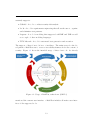
The support of these four tools is no coincidence. The main reason for the development of RiskTest was to create a traceability framework for the context of
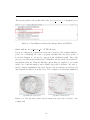
security. Figure 3.1 shows the intended usage of these four tools. As already
Figure 3.1: Usage of RiskTest, taken from: [GBV13]
mentioned the current user interface of RiskTest includes all native user interfaces of the supported tools.
13
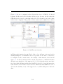
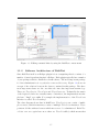
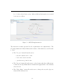
Figure 3.2 shows a configuration that depicts the views of CORAS, ProR and
Papyrus. At the very left border there is the project browser. At the center the
CORAS view is located, on its right is the view of ProR and below both of these
is the view of Papyrus. The position of the views can be adjusted as common
Figure 3.2: RiskTest user interface
in Eclipse-style interface layouts. Each of the tools could run on its own, but by
starting multiple tools in RiskTest it is now possible for the user to edit traces,
for example via the context menu. An example of this interaction is shown in
figure 3.3. As already mentioned the current user interface of RiskTest includes
all native user interfaces of the supported tools. Note that the native user interfaces keep their full functionality since RiskTest loads all tool-specific interactive
buttons and icons if a native view is selected. This means that RiskTest does not
decrease the usability of any of the supported tools, while adding more functionality.
14
Figure 3.3: Editing semantic links by using the RiskTest context menu
3.1.2
Software Architecture of RiskTest
Since RiskTest itself is an Eclipse plugin it is not surprising that it consists of a
number of interdependent plugins for Eclipse. Each plugin typically has a number
of java packages which contain the relevant classes. The most important package
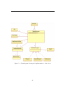
for data administration is org.yakindu.crema.model.tracing. Figure 3.4 shows an
excerpt of the relations between the classes contained in this package. The three
most important classes are the ones that also introduce important terminology.
These are TraceProject, TracePoint and TraceConnector. Technically the names
of the depicted classes are actually names of interfaces, the implementations simply have ”-Impl” as a suffix. For example the implementation of the TracePoint
interface is called TracePointImpl.
The class diagram shows that in RiskTest a TraceProject can consist of multiple resources, which in turn may consist of multiple TracePoint instances. Trace
points model the artifacts between which traces are to be administered. Each TracePoint can once again have more than one TracePointEnd, which means that
15
Figure 3.4: Class diagram of org.yakindu.crema.model.tracing
it can be related to any number of other TracePoint instances. These relations
are modeled by the TraceConnector instances. They relate two TracePointEnd
instances with each other, thus modeling that there is a trace between the two
corresponding trace points. A TraceProject instance can of course have multiple
TraceConnector instances. The TracePointType object provides additional information about the specific trace point it is associated with. Among other things it
contains a string that identifies the tool in which the artifact that is represented
by the trace point was created. This tool is also called the trace point’s provider.
In order to easily extract information out of TraceProject objects or modify them,
there are useful utility classes such as de.fraunhofer.tracing.util.TraceManager
and org.yakindu.crema.model.tracing.util.ModelUtil.
3.2
Requirements Collection
The requirements for the visualization were collected over multiple meetings with
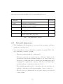
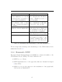
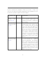
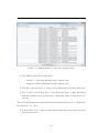
the developers of RiskTest from the Fraunhofer FOKUS institute. Table 3.1 gives
an overview about the different categories of requirements. The requirements of
16
each category are then specified in the corresponding subsection.
Requirements
Category
Data and Appearance
Interaction
Hierarchies
Filtering
Summary
Description
Subsection
Deals with data constraints and the visual rep- 3.2.1
resentation of information
A summary of all the interactive features the vi- 3.2.2
sualization needs to include
Deals with information about hierarchies in the 3.2.3
trace project
A more detailed look on the interactive possibil- 3.2.4
ity of filters
A brief summary containing the most important 3.2.5
aspects of the other categories
Table 3.1: Requirements overview
3.2.1
Data and Appearance
• The Visualization allows the user to view a freely chosen subset of all trace
points of one trace project.
• The chosen subset of trace points will be visualized as a graph. The following constraints or restrictions apply:
– The trace points form the set of all vertices.
– The trace connectors are a part of the set of all edges. It may be the
case that all edges in the visualized graph are also trace connectors,
but it is also possible that they are virtual edges, meaning they cannot
be mapped to a single trace connector. The notion of virtual edges
and their purpose is explained in subsection 3.2.4.
– The visualization must be able to deal with a trace project that contains up to 2000 trace points and any number of trace connectors.
– The trace project contains at most one trace connector for each pair
of trace points.
17
– The trace connectors have no direction, that means if a, b are two trace
points and c is a trace connector between a and b then a is a neighbor
of b and b is a neighbor of a in the resulting graph.
• The providers can be interpreted to be in a hierarchical order, for more
details see subsection 3.2.3.
• The visualized graph can be dynamically changed by employing filter mechanisms. See subsection 3.2.4 for more details.
• Changes to the structure of the graph made in the visualization are automatically applied to the original trace project. See subsection 3.2.2 for
possible modifications of the graph by the user.
• The graph should be automatically drawn in an aesthetic way, so that the
user is able to clearly recognize the traces between the trace points and
confusion is avoided.
• When drawing graph vertices, the following should be considered:
– Each vertex is to be labeled with the name of its corresponding trace
point.
– Each vertex is depicted as the icon of the corresponding provider.
– Additional information considering a trace point can be revealed by
the user. See subsection 3.2.2 for more details.
• When drawing edges, the following should be considered:
– Virtual edges are to be drawn differently than edges that can be
mapped to a trace connector.
– Edges are to be labeled by information contained within, if such information is present.
• As it is explained in subsection 3.2.2 the user will be able to select edges or
vertices. These selected graph components are to be displayed differently
than unselected graph components.
18
3.2.2
Interaction
The visualization allows the user to interact with it. In order to logically describe
the possibilities of interaction, a definition of a view is necessary:
View A view consist of the following things:
• A graph, meaning a set of trace points and a set of edges (either real
trace connectors or virtual edges).
• A set of positions mapping each trace point to a coordinate.
• An edge style specifying how the edges are to be drawn.
In short: a view encompasses all relevant information to create a drawing of a
graph.
• The visualization allows the user to create a view by browsing all trace
points of the trace project and selecting some of them. While browsing,
filter mechanisms can be employed. These filter mechanisms are:
– Name of the trace points (normal substring search)
– Provider of the trace points
• The visualization allows the user to open multiple views and switch between
them.
• The visualization allows the user to interact with views. The possible ways
of interaction are:
– Creation and deletion of edges. If an edge is deleted or created the
trace project is updated, meaning an equivalent trace connector is
deleted or created.
– Dynamic addition and removal of vertices.
– Filter trace points of a certain provider. This is discussed in detail in
subsection 3.2.4.
– It should explicitly not be possible to create or delete trace points via
the visualization.
19
• The visualization allows the user to either select automatic layouts or manually arrange the visualized trace points. Both possibilities can also be
combined, for example an automatic layout algorithm can be applied to
generate a layout which can then be adapted by the user.
• The visualization offers saving and loading options for views.
• The visualization allows the user to reveal additional information for a
vertex. These information include its neighborhood.
3.2.3
Hierarchies
The requirements of the data and appearance category (subsection 3.2.1) already
mentioned that the tools integrated by RiskTest may have a hierarchical connection. This directly leads to the notion of hierarchies in the trace project. A closer
look on these hierarchies is necessary: Trace points are artifacts that belong to
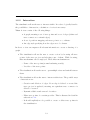
exactly one tool (the provider). Each tool belongs to a domain, for example risk
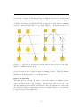
assessment or automatic test generation. In the developing process of a technical
system these domains can usually be considered to be logically ordered (risk assessment is done earlier than test generation). Thus these domains are forming
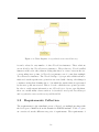
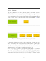
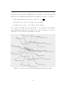
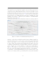
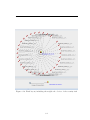
a hierarchy with regard to the specific process in which they were used. An example trace project is given in figure 3.5 where such a hierarchy is depicted. The
trace points are drawn as yellow squares, the trace connectors are drawn as black
lines connecting the trace points. The domains are labeled by the green squares
and sorted from high (top) to low (bottom). This figure gives a typical example
of semantic links in a RiskTest project. The trace points created by CORAS
are artifacts from the security risk analysis, ProR administers test patterns to
ensure the fulfillment of requirements, TTWorkbench is used for automated test
generation and execution.
The intended use of RiskTest depicted in figure 3.1 shows that the process puts
the tools that are currently supported by RiskTest in a hierarchical order: First
security risk analysis is done with the help of CORAS, then ProR is used to find
fitting security test patterns, afterwards Papyrus is used to generate test cases
and finally these test cases are executed by TTWorkbench.
20
Figure 3.5: Hierarchy among the domains
It is important to note that the hierarchy of the tools is dependent on the process that is employed. The same tools may be ordered differently in two distinct
processes.
Hierarchical Trace Project A trace project is hierarchical, if all tools providing the trace points can be put into a logical order (hierarchy).
This logical hierarchy between tools becomes important when filtering is discussed
(see subsection 3.2.4).
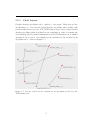
In the example shown in figure 3.5 it is clear that there not only exists a trace
between A and B, but also between A and D as well as A and E (the test cases D
and E cover the security risk A). The above example may lead to the assumption,
that the definition of a trace could be transitively extended. In other words if a, b
and c are trace points and there is a trace between a and b as well as between b
and c then there is a trace between a and c. This would mean that it would be
sufficient to find a path in the resulting graph in order to say for two trace points
21
that they are semantically linked. This looks promising at first but after a more
detailed analysis it becomes clear that it would be a wrong assumption.
Figure 3.5 shows that there is also a path in the trace project leading from A
to C because C and E are connected. C however does not have any semantic
connection to A, since the test pattern that C represents was not used to cover
the security risk represented by A (otherwise there should be a trace connector
between them). This means that it would be wrong to say that A and C are
linked by a trace. Further restrictions are necessary:
Hierarchical path Let G = (T P, T C) be the graph that is formed by a hierarchical trace project, where TP (all trace points ) are the vertices and TC (all
trace connectors) are the edges and let Dom : T P → N be a function that
maps each trace point to a number according to the hierarchical position of
its domain(the highest tool in the hierarchy has the lowest number), then
a hierarchical path from a to b (a, b ∈ T P ) is a sequence S = {tp|tp ∈ T P }
of trace points, with the following constraints:
• |S| > 1
• S0 = a
• S|S|−1 = b
• ∀i ∈ {0, ..., |S| − 2} : (Si , Si + 1) ∈ T C ∧ Dom(Si ) ≤ Dom(Si + 1)
In the example shown in figure 3.5 the path from A to D is a hierarchical path,
since it fulfills the criteria specified above. The path from A to trace point C
is no hierarchical path since the last condition of a hierarchical path is violated.
If the trace project is hierarchical, then it is useful to extend the definition of a
trace to:
Trace Two trace points a and b are connected by a trace if there exists a hierarchical path either from a to b or from b to a.
The notion of hierarchies and this extended definition as well as the concept of
a hierarchical path is needed when filtering is discussed in detail in the next
subsection.
22
3.2.4
Filtering
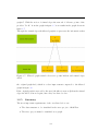
The user is supposed to be able to filter the views by trace point providers.
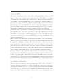
While this does not seem to be a problem at the first glimpse, complications can
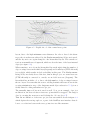
arise. Consider once again the hierarchy depicted in figure 3.5. If trace points
of a provider would be removed without any additional actions then the removal
of the provider ”ProR” would result in the graph depicted in figure 3.6 When
Figure 3.6: Filtered graph with ProR’s trace points hidden
looking at the diagram the beholder could be misled into believing that there
are no traces between any of the depicted trace points. This is of course a false
assumption, since they are just hidden by the filter mechanisms. To avoid this,
the notion of virtual edges that was already mentioned in subsection 3.2.1 is now
applied. The rule for the addition of virtual edges is as follows:
Let G = (T P, T C) be a graph of a view and the graph resulting from a filtering
action is G0 = (T P 0 , T C 0 ) where T P 0 ⊆ T P and T C 0 ⊆ T C. Then ∀(tp1, tp2) ∈
T P 0 × T P 0 add a virtual edge between tp1 and tp2 if (tp1, tp2) ∈
/ T C 0 and there
exists a hierarchical path from either tp1 to tp2 or from tp2 to tp1 in the original
23
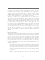
graph G. With the notion of virtual edges the removal of all trace points of the
provider ”ProR” from the graph in figure 3.5 now results in the graph shown in
figure 3.7.
Through the virtual edges the filtered graph now preserves the information that
Figure 3.7: Filtered graph with ProR’s trace points hidden and virtual edges
added
the original graph had, which is a clear improvement compared to the filtered
graph in figure 3.6.
If the original graph is restored by the user (the filter is removed) then the virtual
edges should be removed again, since they are then obsolete.
3.2.5
Summary
The most important requirements of the ones listed above are:
• The data structure to be visualized is the trace project of RiskTest.
• The trace project must be visualized as a graph.
24
• A static display is not enough, the visualization needs to be interactive.
• The trace project can be hierarchical in which case the use of a filter may
lead to the addition of virtual edges in the new graph. This has the goal of
preserving information.
The requirements underline that graph visualization is the central task when
creating an interactive visualization for RiskTest. Therefore the next section
deals with existing graph drawing frameworks and tools.
3.3
Graph Drawing Tools and Frameworks
This thesis is only one of many examples where the visualization of a graph
is the essential problem that needs to be dealt with. Thus there are already
several tools and frameworks that offer graph visualization functionality. This
section gives an overview over some of these and analyzes their usefulness for this
particular problem. Finally one of the solutions is picked. The advantages and
disadvantages refer to the specific task of building a visualization for RiskTest.
They are no general assessments of the tool’s or framework’s usefulness.
3.3.1
Tool: yEd Graph Editor
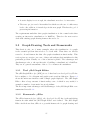
The yEd Graph Editor (see [yED]) is a tool that has been developed by yWorks.
It is a mighty tool for diagram and graph creation and modification. Figure 3.8
shows the main user interface with a simple graph displayed. The yEd Graph
Editor offers a large amount of functionality, some of which is very useful, for
example a number of automatic layout algorithms.
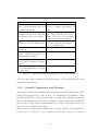
The most important advantages and disadvantages of the yEd Graph Editor are
summarized in table 3.2.
3.3.2
Framework: yFiles
The yFiles framework (see [yFia]), also developed by yWorks, is the underlying
framework with which the yEd Graph Editor was realized. The yEd Graph
Editor itself shows that yFiles is a powerful framework for graph drawing and
25
Figure 3.8: Main user interface of the yEd Graph Editor
that comfortable tools can be created using it. The advantage of the framework
in contrast to the tool is of course that the framework can be used to create
a specialized visualization that is cut down to the exact requirements and no
external tool needs to be employed.
The biggest disadvantage in this context is that yFiles is not free to use ([yFib]). A
license is required. This is such a severe disadvantage in the context of a bachelor
thesis that a further analysis of advantages and disadvantages is obsolete.
3.3.3
Framework: JUNG
The Java Universal Network/Graph Framework (JUNG-framework) is an open
source framework for java (see [JUNa]). It encompasses among other features:
• Basic interfaces like graph, hypergraph, forest, etc. as well as basic implementations of these.
• Algorithms from graph theory, such as shortest path, minimum spanning
tree, but also algorithms from specialized graph theoretic problem domains
like social network analysis.
• Visualization classes that ease the task of drawing graph layouts.
26
Advantages
The yEd graph editor is an already completed tool, so very little effort needs to be spent in order to build a visualization
Very comfortable and intuitive
user interface with a large
amount of graph customization
possibilities
Some automatic layout algorithms are already implemented
Disadvantages
Very difficult or even impossible to integrate into the user interface of RiskTest, needs to be
used externally
Data transfer could be problematic, communication with RiskTest needs to run over files.
Communication is especially difficult when data is changed in
the visualization and the trace
project needs to be updated
Not open-source which means
that extensions are not possible
Direct filtering of the visualized graph not possible to implement, visualized part of the
trace project could only be prefiltered
Table 3.2: Advantages and disadvantages of the yEd Graph Editor
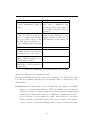
The most important advantages and disadvantages of the JUNG framework are
summarized in table 3.3.
3.3.4
Framework: OGDF
The Open Graph Drawing Framework (OGDF) is a framework similar to the
JUNG-framework (see [OGD]). The major differences are:
• OGDF is a c++ library
• OGDF implements more of the approaches that were discussed in chapter
2 than JUNG
• OGDF does not provide support for the visualization of the graph itself,
only layouts are implemented.
27
Advantages
JUNG is a java framework, so it
can be easily integrated into the
Eclipse environment
Good Documentation: several
examples and tutorials exist that
demonstrate the correct usage
Disadvantages
Visualization needs to be built,
leads to a higher expenditure of
time
Visualization is only embedded
into swing, RiskTest uses SWT,
this could lead to the necessity
of an external swing window
Some automatic layout algo- Several automatic layout aprithms are already implemented proaches discussed in chapter 2
are not implemented
JUNG is a free, open source
framework
Clear and logical software architecture, different interfaces for
different functionalities
Several graph specific algorithms
that could be useful are implemented
Supporting java classes designed
for an easy visualization of graph
layouts exist
Table 3.3: Advantages and disadvantages of the JUNG framework
The most important advantages and disadvantages of the OGDF framework are
summarized in table 3.4.
3.3.5
Overall Comparison and Decision
As the tables listing the advantages and disadvantages already hinted, the JUNG
framework is suited best for the creation of a visualization for RiskTest. While
the yEd Graph Editor offers great usability in dealing with visualized graphs, the
usage of an unchangeable external tool brings too many drawbacks, especially in
the category of data transfer and communication. These drawbacks do not even
arise if an own visualization is built.
yFiles is likely a high quality framework for graph drawing and visualization,
however it not being free to use is unacceptable in the context of a bachelor
28
Advantages
More automatic layout approaches implemented than in
JUNG
OGDF
might
outperform
JUNG. Note that no tests were
made to confirm this assumption. It is purely based on the
fact that properly written c++
code is usually faster than java
code
OGDF is free to use
Good Documentation: several
examples and tutorials exist that
demonstrate the correct usage
Clear and logical software architecture, different interfaces for
different functionalities
Several graph theoretic algorithms that could be useful are
implemented
Disadvantages
OGDF is a c++ library, which
may lead to difficulties and
drawbacks when integrating it
into RiskTest, which is a java application
No built-in support for interactive graph visualization, even
higher amount of time needed
than with the JUNG framework
Table 3.4: Advantages and disadvantages of the OGDF
thesis, especially since free alternatives exist.
Finally the OGDF framework does have two advantages over JUNG, but in the
following it is explained why they are not that important or outweighed by the
disadvantages:
Performance: It is important to keep in mind that algorithms from OGDF
might not even run faster than the JUNG algorithms, as it was already
explained in table 3.4. Even if that is the case though, the requirements
stated that for this bachelor thesis it is sufficient to assume that the trace
project can have at most 2000 trace points. 2000 vertices is a moderate
number in terms of algorithm runtime. There are no bounds on the number
of trace connectors except that multiple trace connectors between the same
29
pair of trace points are not allowed. This results in a maximum number of
1.999.000 edges in the (very unlikely) worst case of a complete graph.
In short this means that the worst possible case of a graph on which to
run algorithms is: G = (V, E) with |V | = 2000 and |E| = 1.999.000.
While 2 million edges is undeniably a large number, runtime for most graph
theoretic algorithms on this graph should still be tolerable, even in a ”slow”
programming language like java. The only restricition is that one might
want to avoid algorithms with O(|E|2 ) time or higher.
While the analysis for the worst case is theoretically interesting, it is highly
unlikely that any graph with that size will ever need to run through a layout
algorithm since viewing all 2000 vertices at once will seldom be the intention
of the user. It is much more likely that only a small subgraph is of interest
in which case the question of performance becomes negligible.
More layout approaches implemented: The availability of fully implemented
layout algorithms does save time, but given a clear specification of the layout
algorithm, implementing it should not take too much time either. JUNG
does already provide some algorithms, which makes the amount of time that
is needed for additional layout algorithm implementations manageable.
In addition JUNG provides utility classes that greatly reduce the effort for
actually visualizing the graph which more than makes up for the possible
effort of implementing a missing layout algorithm.
To sum it up one can say that OGDF does offer some advantages over JUNG,
but they are not relevant in this case. On the other hand, the two advantages
that JUNG has over OGDF (support for visualization and being a java-library)
are very relevant. That means that the JUNG framework is suited best. Now
that the framework that is to be used was determined, it is time to choose useful
graph drawing algorithms the visualization should encompass.
3.4
Graph Drawing Algorithms
Chapter 2 laid out different approaches to graph drawing and categorized them.
Now it is time to revisit those categories and decide whether an algorithm of it
30
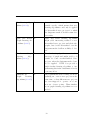
should be included in the visualization. This is done in table 3.5. Each of the
categories from which an algorithm is implemented in the visualization is revisited and the algorithm is explained in detail in chapter 5.
Algorithm cate- Included
gory
Justification
Planar
Graph
Drawing
Algorithms (2.2.2.1)
No
Neither a normal, nor a hierarchical trace
project is assuredly a planar graph, so algorithms would often fail, or result in nonplanar drawings.
Symmetric Graph No
Drawing Algorithms
(2.2.2.2)
It is unclear how many symmetries the algorithms would be able to find in a trace
project. Results from the same algorithm
could strongly differ with different subgraphs. As it was already stated, symmetry can come at the cost of an increased
number in edge crossings, which again hinders readability. Additionally the JUNGframework does not provide an algorithm
specialized on symmetrical layouts, thus
additional time would be needed to implement one.
Hierarchical Graph Yes
Drawing Algorithms
(2.2.2.3)
If a trace project is hierarchical (which
it is in the standard uses of RiskTest)
it fits the requirements of the Sugiyama
method. That means that the algorithm
is specialized to aesthetically draw graphs
of exactly the type the trace project and
all possible subgraphs are. This promises
good results and is worth the effort of implementing it, which is necessary because
JUNG does not provide it.
31
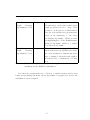
Tree Drawing Algorithms (2.2.2.4)
No
A non-hierarchical trace project is not necessarily acyclic, which means that tree
drawing algorithms could only be applied
for hierarchical trace projects for which
the Sugiyama method should return better results.
Spine and Radial No
Graph Drawing Algorithms (2.2.2.5)
Spine and radial drawing algorithms
might yield interesting results for nonhierarchical trace projects and their subgraphs, but for the hierarchical ones the
Sugiyama method will most likely do better.
Circular
Graph Yes
Drawing
Algorithms (2.2.2.6)
Circular drawing algorithms can visualize
any type of graph and might yield good
results for some non-hierarchical trace
projects, where the Sugiyama method cannot be applied. JUNG does provide a
single-circular drawing algorithm, so implementing this in the visualization barely
costs any effort.
Simultaneous
Graph
Drawing
Algorithms (2.2.2.7)
The requirements state nothing about visualizing two or more trace projects at the
same time, or that different trace projects
are even supposed to operate on a common set of trace points. Thus simultaneous graph drawing algorithms are not
needed.
No
32
Force-Directed
Graph
Drawing
Algorithms (2.2.2.8)
Yes
Force directed drawing algorithms are flexible and tend to yield viable results for any
graph, provided it is not too large. They
promise to work well for non-hierarchical
trace projects and therefore present themselves as an alternative to the circular drawing algorithms. JUNG provides
an implementation of the FruchtermannReingold algorithm, which is a refined
force directed algorithm.
Three-Dimensional
Graph
Drawing
Algorithms (2.2.2.9)
No
Three dimensional drawings call for different user interaction possibilities (for example rotation) than two dimensional drawings, so mixing both in the same application may lead to complications or confusion.
Table 3.5: Graph drawing algorithm categories and their
usefulness for the RiskTest visualization
Now that the requirements were collected, a suitable framework has been
found and promising automatic layout algorithms for graphs were chosen, the
visualization can be designed.
33
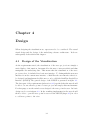
Chapter 4
Design
When designing the visualization two aspects need to be considered: The actual
visual design and the design of the underlying software architecture. Both are
subsequently dealt with in this chapter.
4.1
Design of the Visualization
As the requirements stated, the visualization of the trace project is not simply a
static display of information, but must allow the user to interact with it and thus
manipulate the underlying data. This means that the visualization of the trace
project needs to be included in a basic user interface. To distinguish this new user
interface from the current user interface of RiskTest the user interface that is to
be designed and implemented will from now on be called the RiskTest Graph User
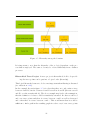
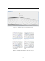
Interface (RTGUI) The general design of the RTGUI is presented in figure 4.1.
The data-part of the requirements (subsection3.2.1) specified that the user should
be able to browse all trace points of a trace project and employ filter mechanisms.
For that purpose another window was designed: the trace point browser. Its basic
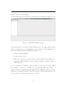
design can be seen in figure 4.2. In the resulting implementation the user should
then be able to open the trace point browser via the RTGUI (fiugre 4.1) in order
to add trace points to the view.
34
Figure 4.1: Basic design of the RiskTest-GraphUI (RTGUI)
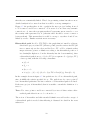
4.2
Design of the Software Architecture
The RTGUI is not only supposed to allow interaction with the layouts, but also
manipulation of the underlying trace project. In order to avoid confusion and
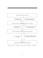
unwanted side effects a good software architecture for dealing with data, its visual
representation and user interaction is needed. The model-view-presenter (MVP)
software pattern offers exactly this by clearly separating visualized data from
the underlying data-model. A slightly modified version of the MVP pattern is
used in the implementation of the RTGUI. The normal MVP pattern only has
one model-class, which is not enough in this context. Two models are needed
because the actual underlying data model is already given through the trace
project of RiskTest but it was already established that the trace project may
differ from the visualized graphs since these may include virtual edges introduced
by filtering mechanisms. The flow of information in the resulting application
is visualized in figure 4.3. As it was pointed out in the analysis, the JUNG
framework does have a natural support for visualization included. This support
35
Figure 4.2: Basic design of the trace point browser
however is only able to interact with the swing library of java, which leads to
the necessity of developing the visualization as a swing application. This is not
problematic for the development of the RTGUI itself since swing offers a large
amount of functionality. It does however have the drawback that the RTGUI
cannot be easily integrated into a window in the existing interface of RiskTest
since that interface uses SWT classes instead of swing. It is however easy to open
the user interface in a second window parallel to the interface of RiskTest. The
only alternative to that would be not to use the classes of JUNG that support
the visualization of graphs which would lead to a much higher expenditure of
time since the functionality of these classes would have to be at least partly
reimplemented into SWT compatible classes.
36
Figure 4.3: Software architecture with regard to the exchange of information
37
Chapter 5
Implementation
This chapter illustrates the results of the implementation of the RTGUI. At first a
closer look on the resulting user interface is taken. The chapter then proceeds with
an enumeration of all packages contained in the eclipse plugin that implements the
RTGUI. Afterwards the usage of the JUNG-framework is explained, followed by
a description of the most important classes and their interactions. This chapter
then concludes with a detailed explanation of the algorithmic core of the RTGUI:
The automatic graph layout algorithms.
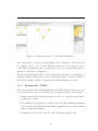
5.1
Resulting User Interface
Chapter 4 introduced the basic design of the RTGUI. The result of the implementation is shown in figures 5.1 and 5.2. The implementation is close to the
actual design. Only the following changes or additions were made:
• The Main-Visualization area consists of multiple tabs that can be opened or
closed by the user. This allows the user to quickly switch between different
views.
• The visualized graphs are drawn inside a window with scrollbars, which
means that graph layouts that are larger than the area of the tab can be
displayed.
• The bottom area displaying additional information only shows the neighbor-
38
hood of the selected trace point. Other additional information is revealed
by mouseover effects.
Figure 5.1: RTGUI implementation
The interactive features specified by the requirements were implemented. The
following enumeration lists all interactive features of the menu bar, as well as the
toolbar.
• The ”Project” menu allows the user to
– save the current view to a file.
– load a new view from a file.
– open the trace point browser.
• The ”Layout” menu allows the user to select between the three different automatic layout algorithms that are included and apply them to the currently
selected view.
• The ”Edge Shape” menu allows the user to change the way the edges are
drawn in the current view.
39
Figure 5.2: Implementation of the trace point browser
• The ”Filter” menu allows the user to
– activate or deactivate filtering in the current view.
– change the filter configuration in the current view.
• The three buttons in the toolbar provide additional view-saving functions.
• The ”Search” text field in the toolbar allows the user to enter any string
and the visualized trace points that contain this string in their name are
selected.
The following enumeration lists all interactive features that are not contained in
the menu bar or toolbar.
• Double-click on one of the view files shown in the left component opens this
view in a new tab.
40
• Left-clicking vertices or edges selects them, shift modifier expands the selection instead of creating a new one.
• Left-clicking a vertex additionally shows its neighborhood (concerning the
trace project) in the bottom component (neighborhood-view). The neighborhoodview may also show trace points that are not included in the currently
selected view.
• Left-clicking on a selected vertex and dragging the mouse moves all selected
vertices.
• Right-Click in a tab opens a context menu, which allows the user to
– create traces.
– delete traces.
– remove trace points (this does not change the trace project, the vertices
are simply no longer depicted in the view).
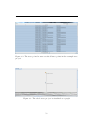
The trace point browser allows the user to browse through all trace points of
the current project. The trace points can be filtered by their name or by the
providing tool. Selected trace points can either be opened in a new view or can
be added to the current one.
5.2
Packages
The implementation is a java eclipse plugin with the following packages:
presenting The presenting package includes all classes that work on the level of
the presenter in the MVP pattern.
dataModels The dataModels package includes all classes that work on the level
of the model in the MVP pattern. Additionally it includes classes that are
needed for the data of some RTGUI components such as the class CustomTableModel which is needed for the trace point browser.
41
layouts The layouts package includes all possible graph layouts that can be
applied to a graph. Most of these are subclasses of classes already existing
in the JUNG framework.
graphUI Standard package for the eclipse plugin that only contains the class
activating the plugin if it is needed, as well as the Main class responsible
for the initialization of the RTGUI and a class defining a basic SWT-window
that provides a button to open the external swing user interface.
extensions The extensions package contains subclasses of already existing classes.
These subclasses usually have a highly specialized purpose, for example
dummy trace points, that act as dummy vertices in a graph, which the
Sugiyama method requires.
interfaceComponents The interfaceComponents package contains all components of the RTGUI windows.
projectConverter The projectConverter package contains a number of utility
classes for the purpose of transforming information obtained by the trace
project into graph structures that the RTGUI requires.
transformers The transformers package contains any classes that implement
the Transformer interface. They are necessary for the correct drawing of
the graph.
util The util package contains utility classes that provide commonly needed functionality.
5.3
Usage of the JUNG Framework
This section gives an overview over the most important interfaces and classes
provided by the JUNG framework and how they are used in the implementation.
Graph The most basic yet important interface is of course the Graph interface.
It defines a large amount of essential methods that allow the manipulation
of the graph as well as tests for adjacency or incidence. JUNG also provides
implementing classes, such as SparseGraph or SparseMultiGraph.
42
Layout The Layout interface is basically a transformer that maps vertices of
a graph to a coordinate. Implementations are the different existing graph
layout algorithms. Used in this visualization are the classes FRLayout and
CircleLayout.
VisualizationServer This interface is the main support for visualization. Its
implementation, VisualizationViewer, takes a graph layout as input and
then visualizes the graph. To do so it subclasses JComponent and therefore
can be put anywhere in a swing window. The interaction with the graph
visualization is highly customizable. The VisualizationViewer class offers
several methods that can modify the default interactive behavior.
RenderContext Each VisualizationViewer has a reference to an object that
implements this interface. The RenderContext offers several more ways
to customize the graph visualization, for example vertex appearance, edge
shape, vertex and edge labeling or edge painting.
For the full Javadoc of the JUNG framework see [JUNb].
5.4
Important Classes and Interactions Between
Them
5.4.1
Realization of the MVP Pattern
The modified MVP pattern that was decided on in the design (see figure 4.3) was
applied. The class interfaceComponents.GraphUI is the main class concerning
the user interface. It integrates all parts of the user interface into one frame.
It is instantiated and called upon by the presenting.Presenter class. This class
handles the logic of the user interface by reacting to user actions, communicating
with the data model and updating the interface via method calls to the GraphUIobject. The dataModels.Model class administers the data to be presented to the
user. It is instantiated and called upon by the presenter object. Furthermore
the dataModels.Model class is responsible for separating visualized data from the
43
original traceability data (trace project). For this purpose it uses the projectConverter.ProjectConverter. This class provides abstract methods in order to
transform information from the trace project into user presentable data.
5.4.2
Bridge to the RiskTest Plugin
Obviously the data model requires access to the data of the RiskTest plugin. All
communication is handled with the help of the de.fraunhofer.tracing.util.TraceManager
class and the org.yakindu.crema.model.tracing.util.ModelUtil class. These classes
access the trace project which contains all traceability related information.
5.4.3
Visualization of the Views
As figure 5.1 already illustrated the views are visualized inside scroll areas. These
scroll areas are visualized inside of tabs so that multiple views can be opened at
the same time. The structure of the implementation can be seen in figure 5.3.
The central class administrating all relevant information for drawing a view is
TabDataStructure. The Presenter class obviously has a number of references
to these, depending on how many views are currently opened. One TabDataStructure object has a reference to a File object, which contains the path of the
corresponding file. A TabDataStructure instance has two layouts, one filtered and
one unfiltered. Which of these layouts is currently being visualized is stored in a
boolean. The filter rules that were applied are stored in the FilterConfig class. A
TabDataStructure object also has a reference to the VisualizationViewer that is
managing the actual visualization and a reference to the GraphZoomScrollPane
that contains the VisualizationViewer. The TabDataStructure instance is also
able to configure the RenderContext of its VisualizationViewer. TabDataStructure objects are configured, initialized and manipulated by the Presenter.
5.5
Graph Layout Algorithms
This section describes the layout algorithms that were implemented in detail.
44
Figure 5.3: Classdiagram showing the implementation of the views
45
5.5.1
Fruchtermann-Reingold Algorithm
The Fruchtermann-Reingold Algorithm is a force-directed graph drawing algorithm. As subsection 2.2.2.8 already explained, force-directed graph drawing
algorithms belong to the most flexible and universal graph drawing algorithms.
The basic concept behind all force-directed drawing algorithms is inspired by
physical forces between the vertices. The vertices will be moved according to the
sum of all forces exerted on them until either they have stabilized and no more
movements occur or a certain number of iterations is exceeded. Then all edges
are drawn (usually as a straight line, but other methods of drawing edges are
possible).
The pseudocode given in algorithm 1 shows the general principle of a force directed algorithm.
The formulas for calculating the attractive and repulsive
Data: Graph G = (V,E) , Integer n
Result: positions: A Map of positions
positions = new Map();
positions = initWithRandomValues();
i=0;
while i < n do
newPositions = new Map();
for v ∈ V do
f = calculateResultingForce(v,positions,G);
newPosition[v] = calculateNewPosition(f,positions[v]);
end
positions = newPositions;
i = i + 1;
end
Algorithm 1: Simple Force-Directed Layout Algorithm
forces, as well as the distance the vertices are to be moved per unit of force can
be adjusted quite a bit. This results in many different force-directed algorithms.
One of them is the Fruchtermann-Reingold algorithm, which is already implemented in the JUNG framework. The Fruchtermann Reingold algorithm has the
additional idea of a global temperature that starts at an initial value and then
linearly decreases. If the temperature is lower, the vertices are moved less distance per unit of force. This means that as the algorithm progresses (and the
46
layout becomes better) the adjustments become smaller. The most important
functions for the Fruchtermann Reingold algorithm in a graph G = (V, E) are:
q
• The optimal distance between two vertices k = C area
|V |
• attractive force: fa (d) = d2 /k ,where d is the distance
• repulsive force: fr (d) = −k 2 /d ,where d is the distance
The complete algorithm is given in algorithm 2. An example layout calculated
by the Fruchtermann-Reingold algorithm can be observed in figure 5.4. For more
information on force-directed algorithms see [Kob07].
Figure 5.4: Layout created by the Fruchtermann-Reingold algorithm
47
Data: Graph G = (V, E);
Integer n; //number of iterations
areaq
= W ∗ L; //W and L are width and length
;
k = area
|V |
for (i=1 to n) do
// calculate replusive forces
for v ∈ V do
// each vertex has two vectors as attributes: .pos and
.disp
v.disp = 0;
for u ∈ V \u do
δ = v.pos − u.pos;
v.disp = v.disp + (δ/|δ|) ∗ fr (|δ|);
end
end
// calculate attractive forces
for e ∈ E do
// each edge is an ordered pair of vertices: .v and .u
δ = e.v.pos − e.u.pos;
e.v.disp = e.v.disp − (δ/|δ|) ∗ fa (|δ|);
e.u.disp = e.u.disp + (δ/|δ|) ∗ fa (|δ|);
end
// update positions, limit maximum displacement to current
temperature and prevent displacement being out of the frame
for v ∈ V do
v.pos = v.pos + (v.disp/|v.disp|) ∗ min(|v.disp|, t);
// Previous line was modified, original source had v.disp
instead of |v.disp| when calculating the minimum
v.pos.x = min(W/2, max(−W/2, v.pos.x));
v.pos.y = min(L/2, max(−L/2, v.pos.y));
end
// reduce temperature
t = cool(t);
end
Algorithm 2: Fruchtermann-Reingold Algorithm, taken from [Kob07]
48
5.5.2
Sugiyama Method
Healy and Nikolov describe the Sugiyama method or Sugiyama framework as the
most popular approach to drawing hierarchical graphs (see [HN07]). In order
to yield good results it requires directed, acyclic graphs as an input. If the
trace project is hierarchical then it can be interpreted as a graph that is nearly
completely acyclic and directed, which makes the Sugiyama method applicable.
The Sugiyama method can be divided into 5 steps:
1. Cycle Removal
2. Layer Assignment
3. Edge Concentration
4. Vertex Ordering
5. x-Coordinate Assignment
The algorithm that is described here is at times a modified version, specifically
created for the context of traceability.
Cycle Removal
The first step, cycle removal, is done to transform an input graph of any kind
into a directed acyclic graph, which the following step requires. The trace project
can be transformed into a directed acyclic graph by employing knowledge about
the domain hierarchies. Therefore the suggested algorithms for cycle removal are
not explained in this thesis. If these methods are of interest they are described
in [HN07]. The transformation of the trace project into a directed acyclic graph
works in the following way:
1. Edges between trace points of different domains are interpreted as directed
edges, the trace point of the higher domain is the head, the other one the
tail.
2. Edges between trace points of the same domain are ignored for the calculation of the Sugiyama method’s layout and are dealt with afterwards. An
49
alternative to this would be to impose directions on these edges as well, but
it is unclear how to do that in a reasonable way. Furthermore, it would
complicate the next step (layer assignment). Additionally, edges between
trace points of the same domain are rare, so ignoring them will probably
not hurt the resulting layout too much.
A disadvantage of this decision is however that the method will now certainly fail to produce good layouts for non-hierarchical trace projects. These
are not dividable into a clear hierarchy, which means that the amount of
layer internal edges will be much higher.
After these two steps the trace project is now a directed acyclic graph, which is
necessary for the next step.
Layer Assignment
The second step, layer assignment, requires a directed acyclic graph G = (V, E)
as an input and returns a proper layering L of G. Important terminology and
explanations (also see [HN07]):
Layering Let L = {L0 , L1 ...Lh } be a partition of the vertex set of a graph
G = (V, E) then L is called a layering of G with the layers L0 , ..., Lh if
∀(u, v) ∈ E if u ∈ Li ∧ v ∈ Lj then i > j.
Vertex rank The layer or rank of a vertex is the number of its corresponding
layer. The function that returns the rank for each vertex is called l. It
short: l(u, L) = i ↔ u ∈ Li .
Edge span The span of the edge e = (u, v) ∈ E in the layering L is defined as
s(e, L) = l(u, L) − l(v, L).
Tight Edges An edge e ∈ E is tight in the layering L if s(e, L) = 1.
Proper Layering A Layering L of a graph G = (V, E) is proper if all edges of
E in L are tight.
It is clear that by categorizing trace points according to their domains and imposing direction on the edges as it was done in step 1 (cycle removal) a layering
50
was already obtained. Thus the layering algorithms described by the Sugiyama
method are not further described in this thesis. They can be consulted in [HN07].
To make a layering proper Healy and Nikolov suggest the introduction of dummy
vertices to split all edges that are not tight. Figure 5.5 shows the creation of a
(a)
(b)
Figure 5.5: (a) shows a non-proper layering, that is made proper by the introduction of dummy vertices in (b)
proper layering from a normal layering via dummy vertices. This algorithm is
intuitive enough that pseudocode is skipped here.
Edge Concentration
The third step is optional. It aims to reduce the number of dummy vertices,
edges and therefore also edge crossings. This however comes at the cost of additional, artificial layers which is undesirable, since the current set of layers has
the desirable feature of reflecting the involved domains. Therefore it is advisable
to skip the step in this application.
51
Vertex Ordering
The vertex ordering step is also often called crossing minimization since it solely
aims to reduce edge crossings between adjacent layers. The number of crossings
is determined by the relative order of the vertices. What is ideally searched for
is a sequence of vertex-permutations (one for each layer) so that the number of
global edge-crossings is minimized. When attempting this one meets the problem
that this is proven to be NP-hard. Even for the comparably simple case of only 2
layers (a bipartite graph), with one layer already having a fixed order of vertices,
the problem of minimizing edge-crossings remains NP-hard (see [HN07]).
Nonetheless there are a number of heuristic and exact methods solving this problem. Running time of the exact ones will of course exponentially increase with
the number of vertices but for small graphs they are viable. The different methods can be categorized into one-layer minimization, two-layer minimization and
multi-layer minimization.
In the context of the RTGUI the greedy-insertion heuristic of the one-layer minimization category is used. While not ideal, the algorithm is simple and can easily
be applied to a multilayered graph. The basic idea is: If V1 and V2 are the two
vertex partitions of a bipartite graph and the order of V1 is fixed, do the following:
Order the vertices of the free layer from left to right by starting with the first
position and insert the vertex v ∈ V2 at the current position if v minimizes the
edge crossings of its incident edges to all edges incident to unchosen vertices.
In order to reduce crossings between all layers this is done iteratively for each pair
of adjacent layers. Additionally, edges between dummy vertices should not be allowed to cross, since this would strongly reduce the readability of these long edges
in the final layout. This is achieved by assigning dummy vertices an already fixed
position when introducing them and ignoring them in the crossing reduction step.
x-Coordinate Assignment
The previous step results in a layered graph with a fixed order of vertices for
each layer. This step is called x-coordinate assignment because most of the times
hierarchies are drawn from top to bottom, meaning that the first layer is drawn
on top, the last one on the bottom. Normally the distance between each of the
layers is the same which only leads to the necessity of now determining an x-
52
coordinate for each vertex (y-coordinate is determined by its layer). Of course
hierarchies can also be drawn left to right. This results in a rotation of 90 degrees,
which means that for hierarchies drawn from left to right, the step x-Coordinate
assignment actually determines the y-coordinates of the vertices. The algorithms
for the coordinate calculation are of course applicable in both cases.
The main goal of this step is to straighten as many edges as possible by vertically (horizontally if left to right) aligning connected vertices. There are different
approaches for this problem. The algorithm that was used here is the algorithm
by Brandes and Koepf [BK01] which Healy and Nikolov describe as one of the
best. The basic idea of the algorithm is to place a vertex at the median of its
lower neighbors’ positions, thus minimizing the sum of the lengths of its incident
edges. This can result in different types of conflicts which need to be resolved.
Note that during this step, the order of the vertices should no longer be changed,
since this was done in the step before. A detailed description of the algorithm
can be looked up in [BK01]. The paper about their algorithm was published in
[MJL01].
Layer internal edges
This step is not present in the Sugiyama framework because the layer assignment
algorithms that are normally applied result in a layering without edges between
vertices of the same layer. In the context of RiskTest these edges were simply
removed for the calculation of the layout. After adding them back to the graph
the layers may become unreadable due to edges intersecting vertices. There are
several possible methods in order to deal with this problem. Note that they
should not significantly alter the layout achieved by the Sugiyama method. The
imaginable solutions are:
• Do nothing, but inform the user that hierarchy internal edges may obstruct
the overview. The user is then able to use the layout as a basis and manually
manipulate it until a satisfying layout is created. This has the advantage of
being both convenient and reasonable in most cases, since hierarchy internal
edges are rare.
• Draw all of the internal edges in an orthogonal way. That way, internal
53
edges may overlap, but at least they do not intersect vertices.
• Move vertices with many layer internal neighbors a bit up or down (in case
of left to right layer drawing: left or right), so that edges no longer overlap
and do not intersect vertices. The difficulty here is to determine a border
on the number of internal neighbors that needs to be exceeded in order for
a vertex to be moved. Additionally if too many vertices are moved by the
same amount and these also share edges, the original problem arises again.
Since it is known that hierarchy internal edges are rare, the first method was
decided on. While it is certainly not ideal to have the user correct flaws in an
automatic layout algorithm, it is a practical solution. After all, the user knows
best what kind of adaptions to the layout make it the most readable for him or her.
The adapted variant of the Sugiyama method described above was implemented
in the RTGUI. Its implementation is done by the class layouts.HierarchialLayout.
An example layout calculated by the Sugiyama method is shown in figure 5.6.
Figure 5.6: Layout created by the Sugiyama method after slight user modifications
54
5.5.3
Circle Layout
Circular drawing algorithms can be applied to any graph. Thus they provide
an alternative to force-directed graph drawing algorithms when dealing with
non-hierarchical trace projects. The JUNG-framework provides a single-circular
drawing algorithm which is included in the visualization. Since it remains unclear which specific algorithm is implemented by the JUNG-framework, no further
description can be given. An example layout calculated by the circular layout
algorithm can be observed in figure 5.7.
Figure 5.7: Layout created by the circular layout algorithm provided by the
JUNG framework
55
Chapter 6
Validation
This chapter validates that the implementation of the RTGUI satisfies the requirements that were collected.
Section 5.1 already explained the interactive features that the implementation
offers. By comparing these with the requirements that were collected in chapter
3 one can already see that all of them were met. To further demonstrate that,
this chapter presents an example usage of the RTGUI. With an example project,
the following shall be achieved via RTGUI:
1. Get a general overview over the traceability structure of the example trace
project.
2. If necessary, manually change the layout of the visualized graph until a clear
and aesthetically pleasing layout is achieved.
3. Save this layout as a view.
4. Modify the example trace project via the RTGUI.
5. Find out how many test cases can be traced to a security risk.
6. Save another view depicting these traces.
At first the RTGUI is opened and it displays its initial state (see figure 6.1). One
can see in the project browser on the left that there are no views saved in the
56
project directory at the moment.
To access the trace project the trace point browser is opened (see figure 6.2). It
Figure 6.1: RTGUI is initially opened
reveals that there are 63 trace points in this project. By employing the filter
at the top-right corner, one can quickly get an overview over the distribution of
these trace points among the different providing tools:
• 1 trace point by CORAS
• 1 trace point by ProR
• The rest of the trace points are almost evenly divided among Eclipse Papyrus and TTWorkbench: 31 trace points by Eclipse Papyrus and 30 by
TTWorkbench.
63 is a comparably low number of trace points for a trace project, but a rather
large number of vertices to visualize in one graph (the higher the number of
vertices, the more complex the graph, thus the more difficult to find a good visualization). Nonetheless it shall be tested how the layout algorithms perform. All
trace points are selected and opened in a new view.
57
Figure 6.2: The trace point browser reveals all trace points in the example trace
project
Figure 6.3: The whole trace project is visualized as a graph
58
The standard layout algorithm that is applied to the traceability graph is the hierarchical layout algorithm (Sugiyama method). The layout algorithm correctly
identifies the hierarchies, the layout does however seem to have the flaw of many
layer internal edges (discussed in subsection 5.5.2) in the third layer which makes
the layout hard to read. Additionally the layout is space consuming due to high
minimum vertex distances. Thus the layout is switched to the FruchtermannReingold layout (see figure 6.4).
The Fruchtermann-Reingold layout immediately returns more pleasing results. It
Figure 6.4: Switch to the Fruchtermann-Reingold layout
manages to reduce the area in which the graph is drawn, resulting in smaller distances the beholder needs to scroll in order to view the whole graph. Additionally
and more importantly one can now identify the traces much better since edges
no longer overlap. The problem for the hierarchical layout seemed to have been
a central trace point in the layer of Papyrus, which is connected to all other trace
points of Papyrus. A look on the neighborhood of this vertex confirms this (see
figure 6.5). The neighborhood can be viewed by selecting the vertex and moving
the border between the visualized graph and the neighborhood view upwards.
A disadvantage of the Fruchtermann-Reingold Layout is that the labels of the
vertices are not always readable, a problem that did not arise in the hierarchical
59
Figure 6.5: Neighborhood of the central trace point
layout, due to the high minimum vertex distances. In order to have both advantages, the view that was achieved by the Fruchtermann-Reingold layout is saved,
and the layout is once again changed to the hierarchical layout. The central vertex is now manually moved upwards, which resolves the issue of the layer internal
edges (see figure 6.6).
What remains to note about the hierarchical layout though is that the number of
edge crossings between the third layer(Papyrus) and fourth layer(TTWorkbench)
is very high, which results in bad readability in this part. The FruchtermannReingold layout clearly showed the fact, that in this project one actual test case
(TTWorkbench) is connected to exactly one modeled test case (Papyrus). The
hierarchical layout fails to do so due to the high number of edge crossings between
the two layers. It seems that the vertex ordering heuristic that was chosen in the
crossing minimization step of the Sugiyama method(see subsection 5.5.2) is not
ideally suited for this particular trace project.
The manually improved layout is saved as well. Now, as an example of project
modification, the traces between four trace points shall be swapped. The swap is
done by creating the new traces and deleting the old ones (see 6.7).
That the modification of the trace project was successful is shown in figure 6.8
which depicts the tracing explorer, a part of the RiskTest user interface that allows to see relations between the trace points in a tree-like structure.
60
Figure 6.6: Manually improved hierarchical Layout
(a) initial state, trace points
of interest are marked
(b) new trace is created via
context menu
(c) old trace is deleted via
context menu
(d) state after the modifications
Figure 6.7: Example modification of the trace project
61
The tracing explorer shows that indeed the fuzzed testcase 8 of Papyrus is now
Figure 6.8: TraceExplorer reflects the changes made via RTGUI
linked with the fuzzed testcase 19 of TTWorkbench.
It is now of interest how many test cases can be traced to the security risk(trace
point of tool CORAS). In order to properly visualize this, the trace points of
ProR and Papyrus do not need to appear in the visualized graph. Since this
trace project reflects the standard use of RiskTest, the providers can be put into
hierarchical relations. Thus the filtering options that are applied do not result
in the loss of any information, since virtual edges will be inserted. In order to
find a compact visualization the circle layout is chosen and the providers ProR
and Papyrus are filtered from the view. The comparison between the unfiltered
(a) unfiltered circle layout
(b) filtered circle layout
Figure 6.9: New layouts to find out how many test cases can be traced to the
security risk
62
layout and the filtered layout in figure 6.9 shows that filtering options combined
with the notion of virtual edges are a powerful approach to strongly reduce complexity while still preserving traceability information. The filtered layout can
now be further improved by moving the security risk to the center (see figure
6.10). Figure 6.10 also shows that the actual neighborhood of the security risk
in the trace project has not changed. The actual neighborhood is depicted in the
neighborhood view below the circle layout.
After applying the filter it is easy to see that all 30 test cases in this trace project
have traces to the security risk.
63
Figure 6.10: Final layout, including the neighborhood view of the security risk
64
Chapter 7
Conclusion and Prospects
This chapter concludes the thesis and gives an overview over possible goals in the
future.
7.1
Conclusion
The goal of this thesis was to create a visualization for dependencies (traces)
between artifacts of different tools in the RiskTest traceability framework.
Traceability data, that means a set of artifacts and a set of links between those,
has the form of a graph which made graph visualization a central topic of this
thesis. It was shown that while there are many categories of graph drawing algorithms, not all of them are viable for the domain of traceability, since some of them
require constraints that are not given in the very general task of visualizing traceability data. The algorithms that were decided on are the Fruchtermann-Reingold
algorithm, a force-directed graph drawing algorithm, the Sugiyama method, a
hierarchical graph drawing algorithm, and a single circular graph drawing algorithm. All of these algorithms were of use during the validation phase, which
implies that the choice was justified.
Furthermore it was established that a static visualization is not sufficient. The visualization was required to have many interactive features which led to the necessity of developing of a basic user interface containing the visualized data. Therefore the RiskTest Graph User Interface (RTGUI) was developed, which combines
the visualization of traceability data with interactive possibilities. To facilitate
65
the development of the RTGUI, several graph drawing frameworks and tools were
inspected out of which the JUNG framework (Java Universal Graph/Network
Framework) was suited best for the development of the RTGUI.
The RTGUI was successfully implemented and integrated into the RiskTest traceability framework which means that the overall goal of this thesis was achieved.
Even though the visualization of traceability data was successfully implemented
there are still relevant topics and open issues that were not extensively dealt with
in this thesis. The last section briefly mentions each of these.
7.2
Prospects
Usability Usability, although undoubtedly an important factor when creating
user interfaces, was not the main topic of this thesis, since its focus was
laid on finding appropriate ways to visualize traceability data. Thus the
usability of the RTGUI could still be enhanced, for example through the
addition of key bindings, drag and drop functionality, improved look and
feel and many other factors that affect usability.
Integration of the RTGUI into the RiskTest Window The necessity of an
external swing window came through JUNG’s natural support for swing.
RiskTest however uses SWT as the basis for visualization. There are some
methods that can be applied to integrate swing components into SWT windows. One could try to apply these here. If they are successful, the RTGUI
could be integrated into the main Window of RiskTest, which would improve the overall handling of RiskTest.
Graph Drawing: Add a labeling algorithm Currently the labels are placed
in default positions by the JUNG framework. In some of the resulting
layouts this can result in the overlapping of labels with other labels, edges
or vertices. This is of course undesirable since it makes the labels hard to
read or can even lead to wrong assumptions if the beholder is confused which
label belongs to which vertex. There are algorithms specifically designed
for the purpose of labeling a map or a drawing of a graph ( see [KGT07]).
66
These algorithms could be reviewed and applied to further improve the
graph layouts.
Graph drawing algorithms for large graphs The layout algorithms that were
chosen work well for small to medium sized graphs. They are practical for
uses in smaller projects or excerpts of larger projects. However, if it is desirable to view the complete traceability graph of a large project at once,
different algorithms will need to be employed. To find out which of these
are viable choices for visualizing large amounts of traceability data could
be a field of study in the future.
67
References
[BCG+ 07] Christoph Buchheim, Markus Chimani, Carsten Gutwenger, Michael
Juenger, and Petra Mutzel. Handbook of Graph Drawing and Visualization (Discrete Mathematics and Its Applications), chapter Crossings and Planarization. In [Tam07], 2007. 9
[BJY] Andreas Bauer, Jan Juerjens, and Yijun Yu. Run-time security traceability for evolving systems. 2008. research report. 5
[BK01] Ulrik Brandes and Boris Koepf. Graph Drawing 9th International
Symposium, chapter Fast and Simple Horizontal Coordinate Assignment. In [MJL01], 2001. 53
[BKI07] Thomas Blaesius, Steven G. Kobourov, and Rutter Ignaz. Handbook
of Graph Drawing and Visualization (Discrete Mathematics and Its
Applications), chapter Simultaneous embedding of planar graphs. In
[Tam07], 2007. 11
[Bra95] F. J. Brandenburg. Graph Drawing: Symposium on Graph Drawing
GD 95 volume 1027 of Lecture Notes in ComputerScience. Springer,
1995. 6, 70
[DG07] Christian A. Duncan and Micheal T. Goodrich. Handbook of Graph
Drawing and Visualization (Discrete Mathematics and Its Applications), chapter Planar Orthogonal and Polyline Drawing Algorithms.
In [Tam07], 2007. 9
68
REFERENCES
[EH07] Peter Eades and Seok-Hee Hong. Handbook of Graph Drawing and
Visualization (Discrete Mathematics and Its Applications), chapter
Symmetric Graph Drawing. In [Tam07], 2007. 10
[GBV13] Juergen Grossmann, Michael Berger, and Johannes Viehmann. A
trace management platform for risk-based security testing, 2013. vi,
2, 4, 5, 13
[GDL07] Emilio Di Giacomo, Walter Didimo, and Giuseppe Liotta. Handbook
of Graph Drawing and Visualization (Discrete Mathematics and Its
Applications), chapter Spine and Radial Drawings. In [Tam07], 2007.
10
[HN07] Patrick Healy and Nikola S. Nikolov. Handbook of Graph Drawing and
Visualization (Discrete Mathematics and Its Applications), chapter
Hierarchical drawing algorithms. In [Tam07], 2007. 8, 10, 49, 50, 51,
52
[JUNa] JUNG Website: http://jung.sourceforge.net/ access date 23.11.2013.
26
[JUNb] JUNG API: http://jung.sourceforge.net/doc/api/index.html access
date 23.11.2013. 43
[KGT07] Konstantinos G. Kakoulis and Ioannis G. Tollis. Handbook of Graph
Drawing and Visualization (Discrete Mathematics and Its Applications), chapter Labelling Algorithms. In [Tam07], 2007. 66
[Kob07] Stephen G. Kobourov. Handbook of Graph Drawing and Visualization
(Discrete Mathematics and Its Applications), chapter Force-Directed
Drawing Algorithms. In [Tam07], 2007. 11, 47, 48
[KS] V. Katta and T. Stalhane. A conceptual model of traceability for
safety systems. 5
[MJL01] Petra Mutzel, Micheal Juenger, and Sebastian Leipert. Graph Drawing
9th International Symposium. 2001. 53, 68
69
REFERENCES
[NR07] Takao Nishizeki and Md. Saidur Rahman. Handbook of Graph Drawing and Visualization (Discrete Mathematics and Its Applications),
chapter Rectangular drawing algorithms. In [Tam07], 2007. 9
[OGD] OGDF Website:
25.11.2013. 27
http://www.ogdf.net/doku.php
access
date
[Pat07] Maurizio Patrignani. Handbook of Graph Drawing and Visualization
(Discrete Mathematics and Its Applications), chapter Planarity testing and embedding. In [Tam07], 2007. 9
[PCJ95a] Helen C. Purchase, Robert F. Cohen, and Murray James. Graph Drawing: Symposium on Graph Drawing GD 95 volume 1027 of Lecture
Notes in ComputerScience, chapter Validating Graph Drawing Aesthetics. In [Bra95], 1995. 6, 7
[PCJ95b] Helen C. Purchase, Robert F. Cohen, and Murray James. Graph Drawing: Symposium on Graph Drawing GD 95 volume 1027 of Lecture
Notes in ComputerScience, chapter Validating Graph Drawing Aesthetics, page 443. In [Bra95], 1995. 7
[Req] Reqtify
Website:
http://www.3ds.com/productsservices/catia/portfolio/geensoft/reqtify/ access date 10.12.2013.
5
[Rha10] IBM Rational Rhapsody Gateway Add on User Manual. IBM Corporation, 2001-2010. 5
[Rus07] Adrian Rusu. Handbook of Graph Drawing and Visualization (Discrete
Mathematics and Its Applications), chapter Tree Drawing Algorithms.
In [Tam07], 2007. 10
[ST07] Janet M. Six and Ioannis G. Tollis. Handbook of Graph Drawing and
Visualization (Discrete Mathematics and Its Applications), chapter
Circular Drawing Algorithms. In [Tam07], 2007. 10
70
REFERENCES
[Tam07] Roberto Tamassia. Handbook of Graph Drawing and Visualization
(Discrete Mathematics and Its Applications). Chapman & Hall/CRC,
2007. 8, 68, 69, 70, 71
[Vis07] Luca Vismara. Handbook of Graph Drawing and Visualization (Discrete Mathematics and Its Applications), chapter Planar Straight-Line
Drawing Algorithms. In [Tam07], 2007. 9
[VW07] Dujmovic. Vida and Sue Whitesides. Handbook of Graph Drawing and
Visualization (Discrete Mathematics and Its Applications), chapter
Three-Dimensional Drawings. In [Tam07], 2007. 11
[yED] yEd Graph Editor Website:
http://www.yworks.com/en/products yed about.html
22.11.2013. 25
access
date
[yFia] yFiles Website: http://www.yworks.com/en/products.html access
date 22.11.2013. 25
[yFib] yFiles Licence info:
http://www.yworks.com/en/products yfiles commercialinfo prices.html
access date 22.11.2013. 26
71