Download D1e Model Compiler

Adaptivity & Control of
Resources in Embedded Systems
D1e
Model Compiler
Responsible: Lund University (ULUND)
Karl-Erik Årzén (ULUND), Anders Nilsson (ULUND),
Carl von Platen (Ericsson AB)
Project Acronym: ACTORS
Project full title: Adaptivity and Control of Resources in Embedded Systems
Proposal/Contract no: ICT-216586
Project Document Number: D1e 1.0 (M24 Release)
Project Document Date: 2010-01-29
Workpackage Contributing to the Project Document: WP1
Deliverable Type and Security: P-RE
Contents
Contents
3
1
Introduction
1.1 Outline of the Report . . . . . . . . . . . . . . . . . . . . . . . . . . . .
5
7
2
Actor Classification
2.1 Properties determined by actor classification . . . . . . . . . . . . . .
2.2 Implementation . . . . . . . . . . . . . . . . . . . . . . . . . . . . . . .
2.3 Experimental Results . . . . . . . . . . . . . . . . . . . . . . . . . . . .
9
9
10
13
3
Scheduling
3.1 Scheduling of SDF networks .
3.2 Scheduling of CSDF networks
3.3 Implementation . . . . . . . .
3.4 Optimization Objectives . . .
.
.
.
.
17
17
19
21
24
4
Actor Merging
4.1 Merge Procedure . . . . . . . . . . . . . . . . . . . . . . . . . . . . . .
4.2 Implementation . . . . . . . . . . . . . . . . . . . . . . . . . . . . . . .
25
25
26
5
Graphical Interface
5.1 Classification . . . . . . . . . . .
5.2 Partitioning . . . . . . . . . . .
5.3 Scheduling . . . . . . . . . . . .
5.4 Merging . . . . . . . . . . . . .
5.5 Manual Network Construction
29
30
31
32
33
35
6
.
.
.
.
.
.
.
.
.
.
.
.
.
Status at M24
.
.
.
.
.
.
.
.
.
.
.
.
.
.
.
.
.
.
.
.
.
.
.
.
.
.
.
.
.
.
.
.
.
.
.
.
.
.
.
.
.
.
.
.
.
.
.
.
.
.
.
.
.
.
.
.
.
.
.
.
.
.
.
.
.
.
.
.
.
.
.
.
.
.
.
.
.
.
.
.
.
.
.
.
.
.
.
.
.
.
.
.
.
.
.
.
.
.
.
.
.
.
.
.
.
.
.
.
.
.
.
.
.
.
.
.
.
.
.
.
.
.
.
.
.
.
.
.
.
.
.
.
.
.
.
.
.
.
.
.
.
.
.
.
.
.
.
.
.
.
.
.
.
.
.
.
.
.
.
.
.
.
.
.
.
.
.
.
.
.
.
.
.
.
.
.
.
.
.
.
.
.
.
.
.
37
Bibliography
39
3
Chapter 1
Introduction
The objective of Task 1.4 in ACTORS is to develop methods and techniques to analyze
and transform a CAL network to allow for efficient execution; in particular to identify subnetworks, which can be scheduled statically and synthesized into units of executable code.
The nature of the deliverable is P (Prototype) and the dissemination level is RE (restricted to a group specified by the consortium). The main body of the deliverable
is a Java application that allows the user to perform the different steps required
to identify statically schedulable sub-networks, calculate schedules, and merge the
involved CAL actors into a larger actor according to a generated schedule. The Java
Model Compiler will eventually be made available in the OpenDF repository. This
report describes the technical background of the model compiler and provides a
user manual. The current version at M24 should be considered a first version. In
spite of this it is, however, almost completely functional, implementing all the required basic functionality.
Being able to identify statically schedulable sub-networks is important in dataflow
modeling, see Deliverable D1a. In many cases applications consist of a large number of, often, quite “small” actors. If these networks are executed as they are, it
would typically lead to large run-time overhead due to extensive token passing
through FIFOs, and possible also due to context switching. If it is possible to merge
these “small” actors into larger actors then the run-time overhead would be significantly reduced.
The model compiler consists of the following main parts:
• actor classification,<
• schedule generation, and
• actor merging,
together with a graphical user interface.
It is only possible to generate static sequential schedules for synchronous dataflow
(SDF) networks and cyclo-static dataflow (CSDF) networks. In order for a network
to be SDF (CSDF) all involved actors must be SDF (CSDF). An actor is SDF if the
number of tokens consumed at each action firing from each input port and the
number of tokens produced at each action firing to each output port are constant.
Similarly, an actor is CSDF if the token consumption rate and production rate at
each port follow a cyclic pattern, e.g., an output port of an actor could have the
pattern 1,0,2, meaning that at the first firing of the actor one token will be generated, at the second firing zero tokens will be generated, at the third firing two
tokens will be generated, at the fourth firing one token will be generated, etc. Us5
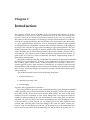
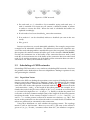
Figure 1.1: The sub-network to the right is part of a non-static cycle.
ing this definition an SDF actor is a special case of a CSDF actor with pattern length
equal to 1.
The task of the actor classifier is to analyze the actors in the network and to
decide if they are static, i.e., statically schedulable, e.g., SDF or CSDF, dynamic, or
timing-dependent. In the static SDF and CSDF case the actor classifier also returns
the token patterns for each port of the actor. The actor classifier is written in Java
and performs the analysis on the .xlim file level.
When the actors are classified it is the responsibility of the user to select a statically schedulable sub-network using the visual feedback provided by the actor classifier. In general any set of interconnected static actors constitutes a sub-network
candidate. However, care must be taken to avoid deadlock situations caused by cycles containing non-static actors as shown in Figure 1.1. The static network to the
left can be merged. However, the two static actors to the right may not be merged.
In order for the actors in sub-network to execute atomically the sufficient number
of tokens must be available on all the input ports of the sub-network. In the example this is not possible since the tokens coming from the dynamic actor only may
be caused by executing the sub-network at the first place. Hence, a deadlock will
be created if the sub-network is merged.
The task of the scheduler is to calculate the minimal repetitive sequential schedule for an actor sub-network, given a certain optimization criterion, e.g., to minimize the total amount of internal buffer space required. The scheduling problem
is formulated as a search problem and solved using the Java-based constraint programming framework JaCoP [1]. The input to the scheduler consists of the subnetwork to be scheduled and the tokens rates of all involved actors. The output
consists of the sequential schedules found and the maximum size required for each
internal “FIFO”.
The task of the actor merger is to merge the sub-network into a single actor given
a sequential schedule and the maximum sizes of the internal “FIFOs”. The actor
merger which also is written in Java operates on the .xlim format. Based on the
XLIMs of the involved actors a new single XLIM is constructed in which the involved actions are executed sequentially according to the schedule and in which
the internal FIFOs are replaced by state variables. From the point of view of the
CAL2C compiler and the CAL run-time system the new XLIM is no different from
ordinary XLIM files generated from “ordinary” actors.
At several parts in the process above user intervention is required. For example, the user needs to select which actors to merge, which optimization criterion
to use, and which of the generated schedules to use. Since dataflow networks are
6
Figure 1.2: The model compiler structure.
Figure 1.3: The ACTORS tool chain.
very graphical in nature it is quite natural to use a graphical user interface for this.
The user interface is implemented in Java using Swing and the JGo graphics library
[2]. The user interface takes an elaborated and flattened XDF file as input. The XDF
format is an XML format where the main tag types are instance and connection. The
instance tags represent actor instances and the connections represent connections
between actor instances. The corresponding network is displayed graphically. Interacting with the network using the mouse the user selects actors and invokes the
classification, scheduling, and merging. In addition it is possible for the user to
manually partition the network. This is required since it is necessary to check that
all the actors that are merged together belong to the same partition.
The structure of the model compiler is shown in Fig. 1.2. The location of the
model compiler in the ACTORS tool chain is shown in Fig. 1.3. The model compiler
takes as input the XDF file and the XLIM files and generates as output a new XDF
file together with new XLIM files for the actors that have been merged together.
1.1
Outline of the Report
Section 2 describes the actor classifier in more detail. The scheduling is described
in Section 3, including how the scheduling problem is represented as a constraint
programming problem. The actor merging is described in Section 4 and the graphical user interface is described in Section 5. Finally, Section 6 describes the current
status of the model compiler and the development that is planned for the period
M24-M36.
7
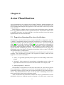
Chapter 2
Actor Classification
Actor classification is the analysis in the Model Compiler, which determines the
opportunities for static scheduling. It allows regions of statically schedulable actors
to be identified and computes the properties of the actors that are necessary to form
static schedules.
In this chapter, we define what we mean by actor classification and we describe
how it is performed. Further, some experimental resuls –classification of the actors
in an MPEG 4 decoder– are presented and we use those results to assess the current
implementation of actor classification.
2.1
Properties determined by actor classification
Classification is closely related to the concept of (dataflow) computation models.
A model of computation imposes particular restrictions on a dataflow graph, by
which analyzability is gained at the expense of expressiveness. Synchronous Dataflow
(SDF) [3] and Cyclo-static Dataflow (CSDF) [4] are two commonly used models of
computation, which allow for static scheduling, but fail to express computations
that require input-dependent schedules. CAL programs are more expressive, but
require dynamic scheduling in general. Actor classification has the purpose of
identifying actors that adhere to particular restrictions (such as those of the SDF
and CSDF models of computation).
The Actor Classifier works by analyzing the internal behavior of each actor in
isolation. The classification is based on the sequence of actions, which an actor
might fire. An actor is classified as
• “static”, if a (possibly periodic) static sequence of action firings can be determined,
• “dynamic”, if the sequence of action firings is dependent on the (values of)
inputs that an actor receives, but not the arrival time of the inputs, and
• “timing-dependent”, otherwise.
Classification is conservative in the sense that unless an actor can be proven
to be independent of timing, it is assumed to be timing-dependent, and unless a
static firing sequence can be found, it is assumed to belong to one of the other two
classes. Any misclassification is thus “on the safe side”: attributing an actor to a
more general class than a perfect classifier would.
Actor classification also determines whether an actor is guaranteed to execute
indefinitely (if given a sufficient amount of inputs) or if it may enter a state, from
9
which no further firings are possible (termination). Indefinite execution is a prerequisite of CSDF (and SDF) models of computation. Again, the results are conservative: possible termination is assumed unless it can be ruled out.
2.1.1
“static” actors
In the case of actors with static firing sequences, results also include the specification of the firing sequence with the production and consumption rates of each step
(an entire period in the case of a CSDF actor). In general, the produced static firing
sequence consists of an initial sequence, which is executed once, and/or a periodic
sequence that can be repeated indefinitely.
Actors with static firing sequences are statically schedulable. It is a CSDF actor
if it has a periodic sequence (executes indefinitely). An SDF actor is a CSDF actor
with period 1. A possible initial sequence corresponds to the concept of initial tokens (“delays” [3]), which is used in the context of CSDF and SDF. A terminating
actor with static firing sequence (i.e. one with no periodic sequence), corresponds
to a one-time execution of the initial sequence. This case is possibly not that common in practice, but it could be a way of providing initial tokens in a dataflow
program.
2.1.2
“dynamic” and “timing-dependent” actors
Actors, which are classified as “dynamic”, have the property that they always produce the same output, given the same inputs. A short motivation is that “dynamic”
actors could be implemented using blocking read operations, by which the requirements of a Kahn-process network [5] are fulfilled. A more detailed discussion is given
in section 2.2.3.
Actors with timing-dependent firing sequences may produce non-deterministic
output, since their effect might depend on the arrival time of inputs.
The current use of actor classification is to provide necessary inputs to static
scheduling. The distinction between dynamic and timing-dependent firing sequences are currently not utilized –they are both negative results. Future enhancements may include quasi-static scheduling of dynamic actors, analyzes and other
transformations that make use of the theory that has been developed for dynamic
dataflow and Kahn-process networks. Such enhancements would rely on the identification of timing-independent and “dynamic” firing sequences.
2.2
Implementation
Actor classification is performed on the so called intermediate representation (XLIM)
of an actor, which is produced by the CAL-compiler front end. This representation
contains a component, which is known as the action scheduler, that is responsible
for the selection of the action to fire in each execution step. This decision is based
on the internal state of the actor, the availability of inputs and, possibly, the value
of inputs. A possible outcome is that the action scheduler signals inability to fire
due to absence of input; we say that the actor is blocked in this case. In addition to
blocking, inability to fire can also be due to termination of the actor (in which case
there will be no further firings).
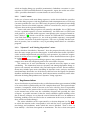
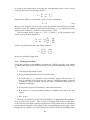
The action scheduler can be represented by a decision diagram (see Fig 2.1a),
in which the interior nodes correspond to tests and the leaves correspond to action firings and conditions, under which the actor is blocked. There is also –at
least initially– a leaf that corresponds to termination. The leaves that correspond
10
to action firings have side-effects: mutation of the internal state and the consumption/production of inputs/outputs –all other nodes are side-effect free. In the first
step of actor classification, the decision diagram is constructed from the intermediate representation of the actor.
The decision diagram can be viewed as a control-flow graph, which is repeated
indefinitely (or until the terminal leaf is reached). Repetition is indicated by the
dashed arrows in Fig 2.1a. A control-flow graph makes lots of traditional compiler
analyses applicable, but not to get overly pessimistic results we have to remove
some of the infeasible paths that are present in the initial incarnation of the controlflow graph. Otherwise, we would have to assume that the firing of a given action
could be followed by that of any of the other actions.
t0
t1
t1
a1
a1
t2
a2
a3
a2
a3
t3
t1
a1
a2
1000 times
a3
t4
t3
a4
a4
a4
(b)
(c)
terminal
(a)
Figure 2.1: Action scheduler represented as (a) decision diagram with added backedges (dashed), (b) a control-flow graph with (some) infeasible paths removed and
(c) a control-flow graph, in which a loop has been summarized into a single node.
2.2.1
Enumeration of state space
In the second step of actor classification, abstract interpretation is employed to enumerate the state space of the actor. As a result, we get an abstraction of the actor’s
internal state that may reach each leaf (each action). Using this information we can
reduce the set of potential successors. In this way we get a more precise controlflow graph, like the one shown in Fig 2.1b. If the terminal leaf was reached during
the enumeration, we must assume that the actor may terminate. Otherwise, we
know that the actor will execute indefinitely.
State-space enumeration starts by evaluating the decision diagram using an abstraction of the initial state. At each interior node, which corresponds to a scheduling test, either one or both of the children are visited –depending on whether the
outcome of the test can be determined or not, given the abstract state. The state,
which has been propagated from the root in this manner, is associated with the
leaves that are reached in this first round of evaluation. Subsequent rounds update the associated state so that we eventually get a meet over all paths solution (e.g.
see [6]).
Leaves with updated states are put on a work list. In each subsequent round
a leaf is picked from the work list, the action’s effect on the state is determined by
abstract interpretation and the decision diagram is again evaluated from the root
using the modified state as input. This enumeration of the state space terminates
when a fixed point has been found. The number of required iterations depends on
properties of the actor and the abstract domain, in which the state is represented.
11
Not only the side-effects of the actions, but also the tests that are performed in
the decision diagram affect the propagation of abstract state: the tested condition
is asserted on the “true branch” and refuted on the “false branch”. For instance, if
the tested condition is x<100, this assertion is made on the “true branch”, by which
precision might be gained (similarly, x>=100 is asserted on the “false branch”).
The implementation of state space enumeration is ignorant of the choice of abstract domain, but presently integer intervals [a,b] is the only implemented one. This
is a good abstraction for “normal” arithmetic operations (+,-,*,/ etc.) and relational
operators. We note that intervals deal with propagation of constant values as a special case. Considerable loss of precision is however caused by bitwise operations
(and, or, xor), which makes intervals less than ideal for code (like the MPEG 4 decoder) that makes heavy use of bit-fields. We consider the implementation of an
additional Boolean domain (bit-vectors) as a remedy.
The implementation of a so called widening [7] is not yet operational, which potentially makes the current implementation impractical. The purpose of widening
is to deal with abstract domains that correspond to very “tall” lattices: precision
is sacrificed to achieve faster analysis. The interval domain is very tall (practically
infinite) and a huge number of iterations might be needed to reach a fixed point.
2.2.2
Loop analysis
A third, not yet implemented, step will perform “traditional” control-flow analyses using the refined control-flow graph and the additional knowledge of the state.
Detection of loops with constant trip-counts is of particular interest, since this case
commonly arises in CSDF actors. Fig 2.1c illustrates the case of a loop, whose tripcount could be determined statically. The absence of the loop analysis step has a
negative impact on the precision of the classification; we elaborate in the assessment, below.
2.2.3
Arriving at the classification
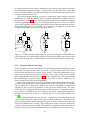
To compute the final result, the actor classification, we consider the set of successors and the scheduling tests that remain (cannot be resolved statically using the
abstract state). Fig 2.2 shows how successors and remaining tests are represented
as per-action decision diagrams. If a remaining test checks for the availability of
input, which at least one of the potential successors does not consume, then the
actor is assumed to be “timing-dependent”. Otherwise, it would be possible to use
blocking read operations, by which the conditions of a Kahn process network are
met, which in turn means that the actor is determinate [5].
initial state, a4
a1, a2
a3
t1
a1
a3
t3
a3
a2
a4
Figure 2.2: Successors
Determining that an actor is not only independent of timing, but also has a
static firing sequence is more intricate. A necessary condition is that each set of
successors (of the initial state and each of the actions) have common production
12
and consumption rates; otherwise, the actor is labeled “dynamic”. For the firing
sequence to be static, each step of the future trajectory of each successor must have
common rates. Otherwise, a static firing sequence cannot be found and the actor is
assumed to be “dynamic”.
We use the sets of successors that are depicted in Fig 2.2 to illustrate the technique. For the first sieve (“dynamic” vs. “timing-dependent”), we consider the
interior (test) nodes: t1 and t3. If either of them tests for availability of input and
the actions, which are reachable from the tests (a1/a2 and a3/a4, respectively), do
not consume that input, the actor is labeled “timing-dependent”.
Otherwise, we proceed with the second sieve (“dynamic” vs. “static”). During
this process, we allow actions with identical consumption and production rates to
be grouped together, into entities called modes [8]. Such a mode can for all purposes
be treated as a single action and we are really looking for a static sequence of mode
firings rather than (original) action firings.
The initial state (and a4) have the successors a1 and a2, which we attempt to
merge into a mode. If we fail to do so (they have different rates), the actor is labeled “dynamic”. The actions a1 and a2 (now merged) have a single successor
a3, which is a trivial case. The action a3 has itself and a4 as successors and an attempt to merge them will be made. Assuming that succeeds, the (now merged)
actions a3 and a4 have the entire set of actions a1, a2, a3 and a4 as successors. If
all of them have the same production and consumption rates (in which case it is
an SDF actor), we merge them into a single mode; a static sequence of length 1 has
been found. If merging fails, the actor is labeled “dynamic”; the outcome of test t3
affects the future consumption/production pattern of the actor, which is why we
cannot schedule it statically.
2.2.4
Producing the static firing sequence
Having reached the verdict of a “static firing sequence”, the actual sequence is also
produced. For finite (terminating) sequences, the entire sequence is given. Infinite
sequences are represented by a (possibly empty) initial sequence, followed by one
period.
We plan to use looped schedules [9], a representation in which repetitions within
the sequence are factored out –otherwise it might be impractical to represent long
sequences (periods). At this point, it is however equally impractical to write an
actor that would result in long sequences (loop analysis is still missing). Figure 2.1c
gives an example, in which a static schedule would have a period of 1002, but a
looped schedule could be really compact.
2.3
Experimental Results
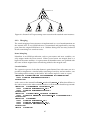
We have classified the actors of the MPEG 4 SP decoder, whose source code is available in the opendf repository1 . It is a decently sized CAL program: consisting of 31
actors, the largest of which (the bit-stream parser) is some 1200 lines of code. It is
also a program that we have gained considerable insight into during the project,
which allows us to make statements about the correctness and the quality of the
classification.
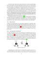
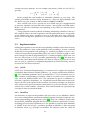
Of the 31 actors, 6 were labeled “static”, 16 were labeled “dynamic” and the
remaining 9 actors were labeled “timing-dependent” (see Fig 2.3). All of the actors
were found to execute indefinitely (given sufficient inputs).
1 http://www.opendf.sourceforge.net
13
By analyzing the actors manually, we found that all misclassification was on
the safe/conservative side. However, five additional “static” actors and one “dynamic” actor were found by manual analysis.
6 actors classified as “static”
5 more actors should be in final classifier
12 actors classified as “dynamic”
1 more actors should be in final classifier
7 actors classified as “timing-dependent”
Figure 2.3: Classification of the actors in the MPEG 4 SP decoder
2.3.1
Actors classified as “dynamic”
Sixteen actors were classified as “dynamic”, four of which were misclassified and
should have received as “static” label.
Loop analysis, which determines constant trip-counts of loops (see Sect 2.2.2),
is required to properly classify DCSplit, Dequant, Interpolate and MBPacker (see
Fig 2.3) as “static”. The classifier currently considers the loop iteration test as
the starting point of two sequences with different consumption/productions rates
(thus the “dynamic” label).
With the exception of these four, misclassified actors, the actors, the remaining
twelve actors that were classified as “dynamic” were correctly classified; each of
them has a firing sequence that depends on the inputs it receives (no static sequence
can be found).
2.3.2
Actors classified as “timing-dependent”
Nine actors were classified as “timing-dependent”, two of which were misclassified: one should have received a “static” label, the other one a “dynamic” label.
Properly classifying Separate (again see Fig 2.3) as “dynamic” requires an enhanced ordering of the tests in the per-mode decision diagrams (c.f. Fig 2.2). In the
current implementation, an input availability test is performed unnecessarily early;
it is located too close to the root. Since there are successors, which are reachable
from that test that do not consume the corresponding input, Separate is classified
as “timing-dependent” (see Sect 2.2.3). However, it would be possible to rearrange
the tests so that only actions, which indeed consume the input, are reachable from
the test.
14
The “static” actor Byte2bit is misclassified as “timing-dependent”. Like Separate, it requires more careful ordering of the tests. Even given that, Byte2bit would
be misclassified (as “dynamic”). Also here loop analysis is required to properly
classify the actor as “static”.
With the exception of the two misclassified actors Separate and Byte2Bit and
some uncertainty regarding the largest actor (ParseHeaders), the remaining six actors that were classified as “timing-dependent” were correctly so; each of them has
a firing sequence that depends on the timing of the inputs, which it receives. Since
manual analysis of ParseHeaders is cumbersome, we do not rule out the possibility
that this actor could in fact be independent of timing (thus “dynamic”).
2.3.3
Required execution time
The complete collection of actors is analyzed in about 13 seconds on a 2.6 GHz
Core2 duo MacBook Pro (the application is single-threaded). One actor, the bitstream parser, stands out –it requires more than 10 seconds— the runner-up takes
about one second and the third longest analysis time is 0.2s. Not only is the decision
diagram of the bit-stream parser by far the largest, a huge number of iterations
(about 12500) was also required to enumerate its state space. None of the other
actors required more than a few hundred iterations (tens of iterations, typically).
We believe that widening of the abstract values would greatly reduce the analysis
time.
2.3.4
Assessment
In conclusion, we find that the classification of the actors in the MPEG 4 decoder
are correct in that it is conservative. Still, precision can be improved: six actors
were attributed to unnecessarily general classes. Two improvements were identified: the (already planned) loop-analysis step and a reordering of input-availability
tests. Given that these two outstanding issues were settled, the classification of the
MPEG4 decoder would be perfect (or nearly so, depending on the status of an actor
that we were unable to completely analyze manually). Still, for other applications
the classification might be less effective, of course.
The lack of widening is a serious problem, since the abstract domain, which we
use, is very tall. Analysis of the MPEG 4 decoder is still practical (requiring 13s on
a standard computer), but it is easy to imagine other applications that would not be
possible to analyze. Completing the implementation of widening is thus essential.
15
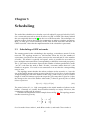
Chapter 3
Scheduling
The task of the scheduler is to calculate a periodic admissible sequential schedule (PASS)
for a connected network in which all actors are SDF or CSDF. The theory behind
this was originally derived in [3] for the case of SDF networks. The techniques are
similar to those used in the Petri Net community in order to calculate invariants.
Here, we first give a brief summary of this, first for SDF networks and then for
CSDF networks. After that the implementation of the scheduler is presented.
3.1
Scheduling of SDF networks
The starting point for the scheduling is the topology, or incidence, matrix Γ of the
network. The topology matrix is a MxN-matrix where the M is the number of
connections (arcs) between the nodes (actors) in the network and N is the number
of nodes. The matrix is typically not square, and it is possible for two nodes to
have multiple interconnections (corresponding to different connected port pairs).
The (i, j)th entry in the matrix represent the number of tokens produced by node
j on arc i each time the node is fired. If node j consumes tokens from arc i, the
number is negative. If a node is not connected to an arc then the corresponding
entry is zero.
The topology matrix decides the token evolution in the network, i.e., how the
size of the buffers changes when an actor is fired. If we let b(n) be a vector of length
M representing the size of the buffers at time step n, and we let v(n) be a vector of
length N with all elements equal to 0 except the ( j)th entry that is equal to 1, then
the change in the size of the buffers when node j is fired is given by the so called
balance equation as
b(n + 1) = b(n) + Γv(n)
(3.1)
The initial value of b, i.e. b(0) corresponds to the initial number of tokens in the
buffers. Currently we assume that all buffers initially are empty. However, this
assumption could easily be relaxed.
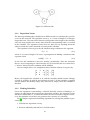
Consider the simple three node example shown in Fig. 3.1. The topology matrix
for this network is given by


2 −1 0
Γ = 0 1 −3 ,
2 0 −3
if we let node A have index 1, node B have index 2, and node C have index 3.
17
Figure 3.1: SDF network.
3.1.1
Repetition Vector
The first step in finding the schedule for an SDF network is to calculate the repetition
vector for the network. The repetition vector, q, is a vector of length N of integers
larger than zero. The sum of the elements corresponds to the length of the schedule
and each entry decides how many times that the corresponding node is executed
in the schedule. The repetition vector, however, does not say anything about the
order in which the nodes should be executed in the schedule.
The repetition vector is given by the smallest integer solution to the equation
Γq = O ,
(3.2)
where O is vector of length N of zeros. A prerequisite for finding a solution to this
equation is that
rank(Γ) = N − 1.
(3.3)
In our case this condition is, however, mainly a technicality. Since the networks
that we are investigating are sub-networks of CAL networks that we assume have
a “correct” behaviour, this condition will be fulfilled.
In our example above it is straightforward to find the solution. It is given by
   

0
3
2 −1 0
0 1 −3 6 = 0
0
2
2 0 −3
Hence, the length of the schedule is 11, and the schedule should contain 3 firings
of node A, 6 firings of node B, and 2 firings of node C. If this schedule is applied
and the buffers are initially empty, they will also be empty when the schedule is
finished.
3.1.2
Finding Schedules
Given the repetition vector finding a schedule basically consists of finding a sequence of node firings that respects the constraints posed by the repetition vector
and that is admissible, i.e., in which the buffer sizes never becomes negative. However, the repetition vector does not guarantee the existence of a schedule.
In [3] a simple sequential scheduling algorithm for solving this problem is presented.
1. Calculate the repetition vector q.
2. Form an arbitrarily ordered list L of all the nodes.
18
Figure 3.2: CSDF network.
3. For each node α ∈ L, schedule α if it is runnable, trying each node once. A
node is runnable if its input arcs all contain a sufficient number of tokens
in order to execute the node. When the node is scheduled the buffers are
updated accordingly.
4. If each node α has been scheduled qα times then terminate.
5. If no node in L can be scheduled, indicate a deadlock (an error in the network).
6. Else, go to 3.
In most cases there are several admissible schedules. For example, our previous
example has 54 admissible schedules. The difference between the schedules consists of the node ordering and how much buffer space that is required. The schedule
that requires the smallest amount of buffer space is the schedule ABBABCBABBC.
For this, the maximum size of the buffer of the connection between node A and
node B is 2, the maximum size of the buffer of the connection between node B and
node C is 3, and the maximum size of the buffer of the connection between node A
and node C is 4. Hence, the maximum value is 9.
3.2
Scheduling of CSDF networks
Scheduling CSDF networks is very similar to scheduling SDF networks. Also, here
the problem can be broken down into two subproblems: finding a repetition vector,
and generating the schedule.
3.2.1
Repetition Vector
Similar to the SDF case finding the repetition vector consists of finding the smallest
integer vector in the nullspace of a “topology” matrix. The difference is the content
of the topology matrix. Consider the CSDF network in Fig. 3.2. We define σij as the
sum of the rates in the token pattern associated with the connection between node
j and connection i, and pij as the length of this token pattern. For example, if we
number the nodes in the previous example A, B, C as 1, 2, 3 and the two connections
as 1, 2 from left to right, then σ11 = 3 and p11 = 2. Finally we define the period Pi of
each node as the least common multiple (lcm) of the length of all the token patterns
involving the node. In the current example we have P1 = 2, P2 = lcm(2, 3) = 6,
and P3 = 3. A token pattern is allowed to contain zero elements, e.g., 1,0,3. This
means in this particular case that when the node is executed for the second time no
tokens are produced (or consumed) at this connection.
Using these definitions we now redefine the topology matrix. The topology
matrix is still an MxN-matrix. However, now the (i, j)th entry in the matrix is
given as Pj σij /pij . If node j consumes tokens from arc i, the number is negative.
19
If a node is not connected to an arc then the corresponding entry is zero. For the
example above the new topology matrix is
3 −15 0
Γ=
.
0 10 −5
Similar to the SDF case a repetition vector, r, is now calculated as
Γr = O ,
(3.4)
However, the elements in this vector are now the number of periods that each node
should execute. The number of individual node firings, i.e., q, is obtained by multiplying each element in r with the corresponding Pi value.
In our example above we have P1 = 2, P2 = 6, and P3 = 3. The repetition vector
for the node periods is obtained as
   
5
0
3 −15 0    
1 = 0
0 10 −5
2
0
and the repetition vector for node firings becomes

  
2∗5
10
q = 6 ∗ 1 =  6 
3∗2
6
Hence, the schedule length is 22.
3.2.2
Finding Schedules
Given the repetition vector finding a schedule for a CSDF network is very similar
to finding the schedule for an SDF network. The same basic algorithm can be used,
i.e.,
1. Calculate the repetition vector q.
2. Form an arbitrarily ordered list L of all the nodes.
3. For each node α ∈ L, schedule α if it is runnable, trying each node once. A
node is runnable if its input arcs all contain a sufficient number of tokens
in order to execute the node. When the node is scheduled the buffers are
updated accordingly.
4. If each node α has been scheduled qα times then terminate.
5. If no node in L can be scheduled, indicate a deadlock (an error in the network).
6. Else, go to 3.
However, the difference is that when the buffers are updated the token patterns
must be taken into account. This is done by keeping track of how many times
each node has been fired and then calculate how many tokens that are consumed
and produced using this value modulus the corresponding pattern length. When
doing this is is useful to use a three-dimensional matrix where the third dimension
20
contains the token patterns. In our example, this matrix, which we will call G is
given by
{1, 2} {−1, −4}
0
G=
0
{1, 3, 1} {−1, −3, −1}
In the example the total number of admissible schedules is very large. The
smallest total buffer size that can be obtained is 8. There are 5670 schedules with
this buffer size. One of them is ABCAAABCAAABBCCAAABCBC.
Since, an SDF actor is just a special case of an CSDF actor, it is straightforward
to generate schedules for networks that contains a mix of SDF and CSDF nodes.
Hence, it is only the calculations corresponding to the CSDF case that have been
implemented.
A large problem with the problem of finding minimizing schedules is that it is
NP-complete. Hence, the time required to solve the problem increases very quickly
as the problem size grows and there is no way of knowing how long it will take.
Hence, when solving these problems it is crucial to be able to set a timeout for the
solver.
3.3
Implementation
Finding the repetition vector and the corresponding schedules can be done in many
ways. The problem is a large search problem so one possibility is to write a tailored
depth-first search program with pruning, etc. Another possibility is to use a conventional integer linear programming (ILP) tool such as CPLEX or gtklp or some
mixed integer non-linear programming tool. A third possibility, which is the one
that was chosen here, is to use constraint programming (CP) [10]. The main reason for this is that Krzysztof Kuchinski, the main developer of JaCoP, the CP tool
that we used, is a professor at neighbour department at Lund University, and also
involved in CAL related activities.
3.3.1
JaCoP
JaCoP (Java Constraint Programming) is a constraint solver engine developed for
constrained finite domain variable problems, e.g., integer and boolean problems,
[1]. The scheduling problems above are modeled as a set of constraints over integer variables corresponding to whether a node is executed or not a certain time
step, and to the different buffer sizes. The constraints are given as arithmetic expressions, equalities, inequalities, etc. Depth-first branch-and-bound search techniques are then used together with constraint consistency techniques to find solutions which satisfy given constraints and optimize a given cost function. JaCoP is
written in Java and variables, constraints, and search methods are represented by
Java objects with associated methods.
3.3.2
MiniZinc
An alternative to represent the problem with Java code is to use MiniZinc. MiniZinc is solver-independent constraint modelling language developed within the constraint programming platform project G12 [11]. There are a number of back-ends
that translate a MiniZinc program into the format needed for a particular CP solver,
including JaCoP. For linear problems it is also possible to translate from MiniZinc
to CPLEX. In the JaCoP case, a problem specified in MiniZinc is first converted
to FlatZinc, where, e.g., all loops are unrolled. The abstract syntax tree (AST) for
21
the FlatZinc program is then interpreted and the corresponding calls to JaCoP constructs are made.
An advantage with using MiniZinc is that the syntax is very user-friendly. For
example, constraints are expressed on a format that is very close to the corresponding mathematical notation, i.e., MiniZinc is highly declarative in nature. A drawback with using MiniZinc is that the JaCoP code generated is not always so efficient
as what can be obtained if the problem is expressed directly in JaCoP Java. In the
current work MiniZinc was used during the development to investigate different
ways of formulating the problem. Once the correct way was found the problem
was rewritten in Java.
As an example the MiniZinc program for finding repetition vectors is shown
below.
int: N;
int: M;
array[1..M, 1..N] of int: Gamma; % Topology matrix
array[1..N] of var 1..1000: q; % Repetition vector
constraint
forall (i in 1..M) (
sum(j in 1..N) (Gamma[i,j]* q(j)) = 0
);
solve minimize sum(i in 1..N)(q[i]);
output [ show(q) ];
% ======= Data ===========
N = 3;
M = 2;
Gamma = [| 2, -3, 0,
| 0, 1, -2|];
Here, the only search variables are the elements in the q vector. Their domain
has been set to 1..1000. The lower bound prevents the search engine from asserting non-positive values for those. The constraint forall loop sets up M equality
constraints where the left hand side in the equalities is given by a series product
between the corresponding row in the topology matrix Gamma and the q vector. The
solver then searches for a solution that minimizes the sum of the elements in the q
vector.
The corresponding JaCoP program is shown below.
public class Model {
Store store;
int[][] Gamma = {{2, -3, 0},
{0, 1, -2}
};
int N = 3;
int M = 2;
public Model() {
}
22
public static void main(String args[]) {
Model run = new Model();
run.model();
}
public void model() {
store = new Store();
Variable zero = new Variable(store,0, 0);
Variable[] q = new Variable[N];
for (int i=0; i<N; i++)
q[i] = new Variable(store, 1, 1000);
for (int i=0; i<M; i++)
store.impose(new SumWeight(q, Gamma[i], zero));
Variable sum = new Variable(store, 0, 1000);
store.impose(new Sum(q,sum);
Search label = new DepthFirstSearch();
SelectChoicePoint select = new SimpleSeelect(q, null,
new IndomainMin());
}
boolean Result = label.labeling(store, select, sum);
}
All variables and constraints are stored in a Store object. The zero value is
represented as a variable with both the minimum and the maximum values equal
to 0. The repetition vector is represented as an array of Variables. In the second
for loop, M SumWeight constraints are imposed. Each of them corresponds to one
of the series products and the value of each series product should be equal to 0.
The values of the sum variable ís given by the sum of the elements in q, through a
Sum constraint. Finally, a depth-first search is set up that attempts to minimize the
value of the sum variable.
3.3.3
Variables and Constraints
The implementation is split up in two parts; one part that calculates the repetition
vector and one part that searches for schedules. Both are implemented in JaCoP.
The search for the repetition vector is based on what was just shown. The search
for schedules is considerably more complex.
The following main optimization variables are used:
• A variable matrix x = new Variable[S][N] where S is the schedule length.
The entry x[s][n] is 1 if node n is executed at step s in the schedule and 0
otherwise.
• A variable matrix b = new Variable[S][M]. The rows in the matrix contain
the size of all the buffers at each step.
• A variable matrix xCumul = new Variable[S][N] that contains the cumulative sum of the elements in the x matrix.
The following main constraints are used:
• Constraints that ensure that each actor only is fired once in each step, i.e., that
the sum of each row in x is equal to 1.
23
• Constraints that update the values in xCumul based on the values in x
• Constraints that ensure that the values in the last row of xCumul equals the
values in the repetition vector, i.e., that each actor has been fired the correct
number of times.
• Constraints that ensure that the initial value of each buffer is equal to 0.
• A number of different constraints that together ensure that each element in
the buffer matrix b is updated according to the balance equation using the
three-dimensional topology matrix G, defined previously. These constraints
use xCumul to decide which values that should be used for the consumption
and production rates.
• Constraints that calculate the maximum value of each buffer and the sum of
these maximum values.
The optimization currently supports three optimization objectives.
• It is possible to search for all admissible schedules.
• It is possible to search for the schedules which minimize the size of the largest
single buffer.
• It is possible to search for the schedules which minimize the sum of the maximum size of all the buffers, i.e. the total buffer space.
In all cases, the search is performed with a timeout that the user can specify.
This is necessary in order to both avoid possibly infinite search times and the associated heap overflow that typically follows. In each optimization it is possible that
no solution can be found. In that case this is reported to the user.
3.4
Optimization Objectives
The current system searches for schedules that in some way minimize the buffer
memory requirements. Another possibility that currently is not implemented is to
also search for schedules that minimize the code space. A possible approach here
is to search for so called single appearance schedules (SAS) [12]. A SAS is a schedule
where each node is executed at one place in the schedule. Repetitive executions are
handled by loops in the schedule.
Another related issue that needs investigation is finding schedules that minimize execution times. Too large buffers and too large code size may degrade the
execution time due to cache effects. If producer and consumer nodes are placed
directly after each other in the schedule, then the possibility to transport tokens directly using processor registers rather than through buffer memory opens up. All
this require the formulation of optimization objectives that catches these requirements and that also can be formulated in JaCoP.
A simple approach that tries to avoid instruction cache misses has been been
implemented. The search for schedules that minimize the buffer space typically
generates several schedules with the same space requirements. These are presented
to the user in a ranking order where schedules with small variability are presented
to the user before schedules with larger variability. The variability of a schedule is
defined as the number of node changes in the schedule. For example, the schedule
AAABB has variability 1 whereas the schedule ABABA has the variability 4.
24
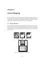
Chapter 4
Actor Merging
The results from the actor classification can be used to merge groups of CSDF actors to a larger actor. The major benefit of actor merging is that runtime overhead
(mainly from synchronization) associated with the FIFO:s connecting actors can be
replaced with internal buffers that do not need any synchronization.
4.1
Merge Procedure
Actor merging is performed on the intermediate XDF/XLIM level, where all actors
in a network have been parametrized and instantiated. It is then safe to perform
transformations on the actors forming the network with no risk for unwanted side
effects due to certain actors being instantiated more than once at several locations
in the network.
Actor_1
Actor_2
Actor_3
Action_1
Action_1
Action_1
Action Schedule
Action Schedule
Action_2
Action Schedule
MergedActor
Actor_1_Action_1
Actor_1_Action_2
Actor_2_Action_1
Actor_3_Action_1
MergedActor_ActionSchedule
Actor_1_Action Schedule
Actor_2_Action Schedule
Actor_3_Action Schedule
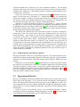
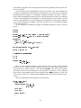
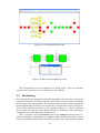
Figure 4.1: Merging three actors into one.
25
4.1.1
Actions
The procedure to merge two actors into one is as follows. First collect all actions
from the actors to be merged and put them as actions in a new actor, see Fig. 4.1.
Search all connections in the network for connections between the actors to be
merged. If a connection between two actors is found, create a corresponding circular buffer in the new actor and replace writes, reads, and peeks on the FIFO queue
with accesses to this buffer. Then remove the connection from the network description since it will no longer be used.
4.1.2
Action Schedule
The process of merging two action schedules into one is a little bit trickier than the
merging of actions. We want to keep the parts of the action schedules that concern
the state of an actor, such as guards and priorities. On the other hand, since we
have defined a static schedule for the actions of the merged actor there is no need
to keep checks for available tokens on internal input queues. If there are enough
tokens waiting on the input queues of the merged actor we know that it is safe to
execute actions according to the decided schedule without any risk of running into
deadlock situations because of a lack of tokens.
A new action scheduler is constructed as follows. A necessary condition to fire
the merged actor is that there are enough tokens available on the inports such that a
complete period of the static schedule may be executed. The action scheduler consists of an outer infinite loop with wait conditions that ensure that enough input
tokens, as well as queue room for output tokens, are available. Inside this outer
loop we simply list the action schedulers from the original actors exactly as they
come in the static schedule, with token queue checks replaced with boolean constants. Note that one cycle in the static schedule may very well mean that some
actors are executed multiple times.
4.2
Implementation
Using a local state-of-art compiler construction tool, JastAdd [13], we have built
compilers for both XDF and XLIM intermediate formats. Using the aspect-oriented
features of JastAdd we can then add new functionality to the compilers in a modular fashion.
4.2.1
Runtime Structures
When a CAL network is opened by a user, the XDF network description is parsed
and an abstract syntax tree (AST) representing the contents is constructed. The
xdf contains a topological description of an actor network, which actors that are
part of it and how they are interconnected. When more detailed information is
needed about an actor, such as classification and actor merging, an instance of the
XLIM compiler is instantiated in order to parse the relevant XLIM actor description.
The resulting XLIM AST is then attached as a sub-tree in the XDF tree for future
references. Loosely one can say that the final fully populated tree has got the trunk
and branches from the XDF while some of the twigs and leaves come from different
XLIM descriptions, see Fig. 4.2.
26
ActorNetwork.xdf
Actor_1.xlim
Actor_2.xlim
Actor_3.xlim
Actor_4.xlim
Figure 4.2: Internal AST representing actor network with attached actor instances.
4.2.2
Merging
The actual merging of actor instances is implemented as a set of transformations on
the internal AST. A new XLIM sub-tree is instantiated and populated by moving
parts from the original XLIM trees to it. Without diving into too many technical
details some things are worth to notice.
Name Mangling
Identifiers in an XLIM specification, such as port names and state variables, are
only unique inside the actor context. When several actors are merged there is a
high risk for name conflicts. As a precaution all identifier names are qualified with
the name of their original actor when being added to the merged actor.
Circular Buffers
The expressive power of the xlim format is quite limited, but with some care it is
possible to implement a circular buffer consisting of an array and two indices, one
for reading and for writing to the buffer. We can then replace a write to a port:
< operation kind = " pinWrite " portName = " Out " style = " simple " >
< port dir = " in " source = " sourceVar " / >
</ operation >
with a write to the internal buffer buf_0 indexed by outIx_0. What then follows is
the code to increase the index and the check to see if the index should wrap around:
< operation kind = " assign " target = " buf_0 " >
< port dir = " in " source = " outIx_0 " / >
< port dir = " in " source = " sourceVar " / >
</ operation >
< operation kind = " $ literal_Integer " value = " 1 " >
< port dir = " out " size = " 32 " source = " one_0 " typeName = " int " / >
</ operation >
< operation kind = " add " >
< port dir = " in " source = " one_0 " / >
< port dir = " in " source = " outIx_0 " / >
< port dir = " out " source = " outIx_0 " / >
</ operation >
< module kind = " if " >
27
< module decision = " decision_0 " kind = " test " >
< operation kind = " $ literal_Integer " value = " 3 " >
< port dir = " out " size = " 32 " source = " one_0 " typeName = " int " / >
</ operation >
< operation kind = " $ geq " >
< port dir = " in " source = " outIx_0 " / >
< port dir = " in " source = " bufSize_0 " / >
< port dir = " out " source = " bufTest_0 " / >
</ operation >
</ module >
< module kind = " then " >
< operation kind = " $ literal_Integer " value = " 0 " >
< port dir = " out " size = " 32 " source = " bufSize_0 " typeName = " int " / >
</ operation >
< operation kind = " assign " >
< port dir = " in " source = " outIx_0 " / >
< port dir = " in " source = " bufSize_0 " / >
< port dir = " out " source = " bufTest_0 " / >
</ operation >
</ module >
</ module >
Note that there are no checks if there is room in the buffer before writing a new
value to it. From the actor classification and static scheduling we know the maximum amount of tokens that may need to be buffered at any moment, and have
declared the buffer to be large enough.
28
Chapter 5
Graphical Interface
The graphical user interface is implemented in Java, using Swing and the graphical
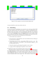
library JGo [2]. The basic GUI of the model compiler is shown in Fig.5.1. The first
thing that the user does is to open an elaborated and flattened XDF file using the
Open action or toolbar button. This opens a file browser through which the user
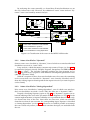
selects which file to open.
The XDF file is read and parsed using the JastAdd compilation framework and
an abstract syntax tree (AST) is created from the XML representation. An advantage of using JastAdd for this compared to, e.g., DOM or JDOM, is that Java
classes are automatically created for all XML tags and attributes. Also, the aspectorientation and reference attributes of JastAdd greatly simplifies all AST-based operations. XDF files contain two main tag types: instance and connection. The instance tag corresponds to an actor instance and the connection tag to a connection
between two ports. After the creation of the AST graphical objects corresponding to
the actor instances are automatically created and placed on a diagram using auto-
Figure 5.1: The basic model compiler GUI.
29
Figure 5.2: Automatic layout of the idct1d CAL network.
matic layout. The layout places all source actors (actors with only output ports) to
the left in the diagram and all sink actors (actors with only input ports) to the right
in the diagram. The remaining actors are placed at a location whose x-coordinate
depends on how large share of the input ports that are connected to actors already
placed to the left of the current actor.
An example of the automatic layout for the idct1d network is shown in Fig.5.2.
Although the layout algorithm is not perfect, it works sufficiently well for its purpose. Also, if the user is not satisfied with the layout he/she can move the actors
and the connections using the mouse. Also, when the mouse is moved over an actor all the actors that this actor is connected to are highlighted. Similarily, when the
mouse is moved over a connection the connection is highlighted.
5.1
Classification
Using the Classify action from the Compile menu all the actors in the diagram are
classified. Static actors are shown in green, dynamic actors are shown in yellow,
and time-dependent actors are shown in red. The latter class also contains actors
which were not successfully classified as either static or dynamic, although they
might in reality belong to one of these classes.
The classification also returns the token patterns for all the ports of the static
SDF/CSDF actors. These can be viewed by selecting the Rates action from the
menu obtained by clicking on an actor. In the popup window shown it is also
possible to manually edit the token patterns, should that be necessary.
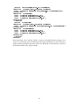
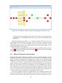
The result obtained when classifying the MPEG SP decoder is shown in Fig. 5.3.
The green actors correspond to the SDF/CSDF idct1d sub-network. In Fig. 5.4 the
popup window showing the rates for the ports of the ShuffleFly_0 actor instance is
shown.
30
Figure 5.3: Classified MPEG decoder
Figure 5.4: Rates of the ShuffleFly_0 actor.
The classification needs the XLIM files for all the actors. They are currently
assumed to be located in the same directory as the XDF file.
5.2
Partitioning
It is assumed that the merging of statically schedulable sub-networks is performed
after the partitioning. The reason for this is that all the actors involved in a merging
must belong to the same partition. The model compiler provides simple support for
manual partitioning. In order to invoke this the user must first select a set of actors.
This is done using the normal way for graphical editors, i.e. either by clicking
on the actors one after the other while pressing the CTRL-key or by outlining a
rectangular area on the diagram with the mouse.
Once a selection exists the Partition action in the Compile menu becomes enabled. Selecting the action brings up a popup window through which the user can
enter the partition number for the currently selected actors. The partition number
31
Figure 5.5: The repetition vector for the idct1d subnetwork.
is shown in bold face at the center of the actor icon.
5.3
Scheduling
In order to invoke the scheduling the user must first select which green SDF/CSDF
actors that should be part of the sub-network. A merge can potentially be performed as soon as two “green” actors are connected to each other. The selection of
the actors is done in the same way as in the partitioning. Once the user has selected
a set of actors the Schedule action in the Compile menu becomes enabled. When
the user selects this action the calculation of the repetition vector for the network is
performed. The operations that are performed are the following:
1. The selected actors are indexed.
2. The connections in which both the source actor and the sink actor belong to
the selected set are indexed.
3. The topology matrix for the corresponding CSDF network is set up. This
includes calculating the node periods, Pi , the token pattern lengths, pij , and
the token pattern sums σij .
4. The JacoP method for generating the repetition vector is called.
5. A popup window displaying the repetition vector is shown.
The displayed window for the idct1d network is shown in Fig. 5.5.
The popup window contains three buttons. By clicking on the ReSelect button
the window disappears and the user may select another set of actors. By clicking
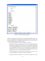
on the Objectives button a new popup window appears. Here, the user can select
which optimization objective to use, set the length of the timeout interval, and
select the identifier name for the merged actors. The situation is shown in Fig. 5.6.
32
Figure 5.6: The objectives popup window.
Finally, by selecting the Generate button the schedules for the current subnetwork are generated according to the currently chosen optimization objective.
The following operations are performed:
1. The three-dimensional topology matrix G is set up.
2. A matrix containing the length of the token patterns for all connections and
nodes is set up.
3. The JaCoP method for generating the schedule is called.
4. A popup window displaying the value of the cost function, the generated
schedules, and the maximum buffers for each schedule is shown. If the timeout has occurred this is indicated. In that case the schedule set only contains
the schedules that have been found within that time. In the case the search
does not succeed finding a solution this is also displayed.
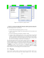
The generated popup window for the idct1d example is shown in Fig. 5.7. The optimization objective here is to minimize the maximum buffer sizes. The minimum
cost that could be obtained was 2 and 7128 schedules where found before the timeout occurred. The schedules are presented on text form ranked according to their
variability.
The popup window contains four buttons. The ReSelect, Generate, and Objectives buttons have the same meaning as in the previous window. The Merge
button initiates the actual merging of the selected sub-network.
5.4
Merging
If the schedule display window contains more than one schedule, which is normally the case, the user first must select which schedule to use. This is done
33
Figure 5.7: The schedule popup window.
through a small popup window where the corresponding schedule number is entered. A prerequisite for the merging to be allowed is that all the involved actors
have been assigned to the same partition. If that is not the case an error message is
displayed and the merging operation is aborted.
The following operations are performed during the merging.
1. The number of tokens that must be present on each of the input ports to the
merged actor in order for the merged actor to be executable is determined.
This is done by going through each of the actors involved and checking, using
the corresponding token patterns, how many tokens that are needed for the
actor to be able to execute as many times as required by the schedule. This
information is necessary since the merged actor is intended to be executed as
a single piece of code, i.e., it may not wait for any tokens.
2. The actor merging code is called with the schedule, the maximum sizes of
each internal buffer, and the input port tokens as arguments.
3. The graphical diagram is updated. The subnetwork is replaced by a single
34
Figure 5.8: The MPEG decoder network after merging the idct1d network.
actor with the corresponding connections. The name of the merged actor is
decided by the user through the Objectives menu, or by manual editing of the
name text.
Repeated merging is possible, i.e., an already merged actor can be part of a
sub-network that is selected for merging. There is, however, currently no undo
functionality. If the user is not satisfied with the performance obtained with the
currently merged actors then the entire process has to be started again, i.e., the
original XDF file has to be opened.
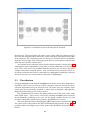
The result after merging the idct1d sub-network in the MPEG-decoder is shown
in Fig. 5.8. This figure should be compared to Fig. 5.3 that shows the corresponding
network before the merging.
5.5
Manual Network Construction
Using the New action toolbar it is possible to create an empty diagram. On this
diagram it is possible to manually create an actor network. The intended use for
this functionality is primarily for debugging the scheduler. By selecting the Open
Palette action from the File menu a palette frame is shown. This frame contains
a skeleton actor instance. Using mouse-based drag-and-drop the user can create
copies of the actor on his diagram. The actors can be moved and resized. Using the
mouse the actor name can be set. By clicking on an actor an Actor menu is shown
from which the user can add and remove input and output ports. Using the mouse
the user can then connect the actor instances and give names to the ports. In this
way a test network can be created. After manually setting the rates for all the ports,
a sub-network can be selected and the scheduling can be invoked.
The model compiler editor has support for the most common graphical edit
operations including cut, copy, paste, delete, select all, move to front, move to back,
zoom in, zoom out, zoom to fit, zoom to normal size, and show a diagram overview.
35
The individual diagram frames can be iconized and maximized, and have both
horizontal and vertical scrollbars.
36
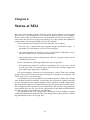
Chapter 6
Status at M24
The status of the model compiler at M24 is good. All the subparts are functional.
However, the actor merging has not yet been integrated with the CAL compiler.
Hence, at this stage we cannot present any quantitative results of how much execution time that can be saved by actor merging. It is also possible that additional
optimizations of the merged XLIM code may be required.
The remaining issues related to the action classifier are as follows:
• The state space enumeration only supports integer and Boolean types. A
possibility is to add support also for real-valued types.
• The implementation of widening is not yet operational. Widening is necessary to avoid the risk of very long execution time.
• Loop analysis has not been implemented. This has a negative impact on the
classification precision.
For the scheduler the following additional issues are possible:
• The optimization objectives could be extended to also cover issues related
to code space and/or execution speed. One such issue could be support for
generating single appearance schedules.
The actor merging is currently in a first prototype version. Here, the resulting
merged actors must be analyzed and performance evaluations are required. The
GUI is more or less in its final shape.
A remaining issue is the integration of the model compiler with the CAL Design
Suite and the OpenDF toolchain, in particular the integration with the run-time
system. Already now the model compiler is able to generate an XML configuration
file (with the file extension .xcf) that will be used as an input to the run-time system.
The configuration file specifies how the individual actor instances are partitioned
and whether there are any special size requirements on the different FIFO buffers
that the run-time needs to take into consideration.
The integration with CAL Design suite will consist of the possibility to obtain
partitioning information from from the CAL Design Suite and to provide scheduling information to the CAL Design Tool.
37
Bibliography
[1]
K. Kuchcinski, “Constraints-driven scheduling and resource assignment,”
ACM Trans. Des. Autom. Electron. Syst., vol. 8, no. 3, pp. 355–383, 2003.
[2]
JGo, “http://www.nwoods.com.” URL, 2010.
[3]
E.A.Lee and D.G.Messerschmitt, “Static scheduling of synchronous data flow
programs for digital signal processing,” IEEE Trans. Comput., vol. 36, pp. 24–
35, Jan 1987.
[4]
G. Bilsen, M. Engels, R. Lauwereins, and J. Peperstraete, “Cyclo-static
dataflow,” IEEE Trans. Signal Processing, vol. 44, no. 2, pp. 397–408, 1996.
[5]
G. Kahn, “The semantics of simple language for parallel programming,” in
IFIP Congress ’74, pp. 471–475, 1974.
[6]
A. V. Aho, R. Sethi, and J. D. Ullman, Compilers, principles, techniques, and tools.
Addison Wesley, 1985.
[7]
P. Cousot and R. Cousot, “Abstract interpretation: a unified lattice model for
static analysis of programs by construction or approximation of fixpoints,” in
POPL ’77: Proceedings of the 4th ACM SIGACT-SIGPLAN symposium on Principles of programming languages, (New York, NY, USA), pp. 238–252, ACM, 1977.
[8]
W. Plishker, N. Sane, M. Kiemb, K. Anand, and S. S. Bhattacharyya, “Functional dif for rapid prototyping,” in RSP ’08: Proceedings of the 2008 The 19th
IEEE/IFIP International Symposium on Rapid System Prototyping, (Washington,
DC, USA), pp. 17–23, IEEE Computer Society, 2008.
[9]
S. Bhattacharyya and E. A. Lee, “Looped schedules for dataflow descriptions
of multirate dsp algorithms,” Tech. Rep. UCB/ERL M93/37, EECS Department, University of California, Berkeley, 1993.
[10] K. Mariott and P. Stuckey, Programming with Constraints: An Introduction. The
MIT Press, 1998.
[11] N. Nethercote, P. Stuckey, R. Becket, S. Brand, G. Duck, and G. Tack, “MiniZinc: Towards a standard CP modelling language,” in Proceedings of the 13th International Conference on Principles and Practice of Constraint Programming, LNCS
4741, 529-543. Springer-Verlag, 2007.
[12] S. Bhattacharyya, P. Murthy, and E. Lee, Software Synthesis from Dataflow
Graphs. Kluwer Academic Publishers, Norwell MA, 1996.
[13] T. Ekman and G. Hedin, “The JastAdd System - modular extensible compiler
construction,” Science of Computer Programming, vol. 69, pp. 14–26, October
2007.
39