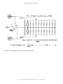
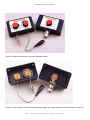
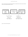
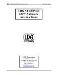
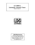
Download How to Evaluate Your Antenna Tuner Part 1

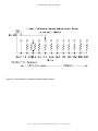
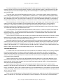
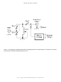
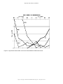
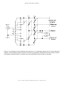
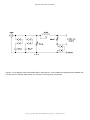
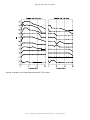
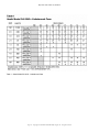
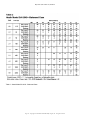
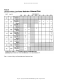
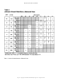
April 1995 QST Volume 79, Number 4
How to Evaluate Your Antenna Tuner⎯Part 1
With some simple low-power measurements you can learn a lot about your antenna tuner.
There may be some real surprises.
By Frank Witt, AI1H
20 Chatham Road
Andover, MA 01810
Antenna tuners add a great deal of flexibility to our stations by converting the antenna system impedance to the
unbalanced 50-Ω load required by modern transceivers. Used properly, an antenna tuner allows us to use one antenna on
several bands. A tuner with a balanced output can convert a balanced antenna into an unbalanced 50- Ω load.
In contrast to most ham equipment, older antenna tuners are still quite useful. Modern ones have some frills like
built-in power and SWR meters and some useful switches, but antique tuners are performing well in ham shacks around
the world.
Unfortunately, we often don’t know much about these very simple and useful devices. An antenna tuner can usually
be adjusted so that the transmitter “sees 50 Ω,” but then what do you have? The specifications of most commercial
antenna tuners are lacking in detail. Some of the things we would like to know about our antenna tuners are as follows:
• Tuning range. What range of impedance can the tuner convert to 50 Ω for each band? Is the range different for
unbalanced and balanced loads? What tuner settings are needed for various bands and loads?
• Loss. How much loss does the antenna tuner introduce into the antenna system? Losses in antenna tuners have been
mentioned recently in QST.1 2 3
• SWR bandwidth. How far from the frequency where SWR = 1:1 can I move before the SWR exceeds some limit, say
1.5:1? More SWR bandwidth usually means less critical tuning.
• Output balance. Is the balanced output truly balanced?
• Power limit. What is the maximum power the tuner will handle for various load conditions?
• Harmonic attenuation. What attenuation of transmitter harmonics can I expect from the tuner, if any?
Except for the last two attributes, everything may be measured by using a low-power SWR tester. Several
manufacturers sell potentially suitable stand-alone SWR measuring instruments. 4 5 6
In this article, I will describe the method for making a comprehensive set of measurements on an antenna tuner. The
concept is simple. A known load impedance is connected to the output terminals, and the low-power SWR tester is
connected to the input terminals. The procedures for finding tuning range, SWR bandwidth and output balance are
straightforward. Some simple analysis is needed to find the loss.
Low-Power SWR Testers
In their simplest form, low-power SWR testers contain a low-power RF signal source and a 50- Ω SWR bridge. Some
also contain a frequency counter or a frequency synthesizer. These units operate with only a few milliwatts of power, and
this adds enormously to their utility. Antenna tuner tests may be performed on antenna systems outside the amateur
bands and only low-power load components are needed. A high-power dummy load is not needed to evaluate high-power
antenna tuners!
The accuracy of the low-power SWR tester must be high enough to obtain meaningful data. We will be using data in
the SWR range between 1:1 and 2.4:1, so it’s important that the instrument be accurate in that range. In Part 2, I’ll show
how to determine the accuracy.
Antenna Tuner Loads
Page 1 - Copyright © 1996 American Radio Relay League, Inc. All rights reserved
April 1995 QST Volume 79, Number 4
I evaluate antenna tuners using switchable resistive loads. These cover the range of impedances that might be
encountered in a typical installation. For unbalanced loads, the tuner design center is assumed to be a 50- Ω resistive
termination. If the load at the output of the tuner is 50 Ω, then a 2:1 SWR load is either 25 Ω or 100 Ω; a 4:1 SWR load is
either 12.5 Ω or 200 Ω, etc. Since I’ve seen some antenna tuners specified to tune loads with SWR up to 10:1, I decided
to test with SWR up to 16:1; that is, resistive loads between 3.125 Ω (50/16) and 800 Ω (50×16).
The loads in my test boxes are pure resistances, even though a more comprehensive test would include
complex-impe-dance loads. For example, a load of 40 ± j30 Ω would also yield a 2:1 SWR. For most situations, however,
an antenna tuner may be satisfactorily characterized using only resistive loads. A method for doing a more comprehensive
test will be covered in Part 2.
Most modern antenna tuners include a built-in 4:1 balun for balanced loads. The tuner design center for balanced
loads is assumed to be 200 Ω. To cover the full 16:1 SWR range, the range for balanced loads is from 12.5 Ω (200/16) to
3200 Ω (200×16). To test for output balance, there is access to the center taps of the balanced loads.
The complete set of terminations is shown in Table 1. Notice that all load resistance values are in a geometric
progression. Each resistance is related by a factor of 2 (or 1/2) to its adjacent neighbors. The reason for this arrangement
will become evident when I describe the method for measuring loss. Incidentally, a ratio of 2:1 is not mandatory ⎯I could
have chosen other ratios, such as 1.5:1 or 3:1, if I wanted to compress or expand the test load range.
Geometric Resistance Boxes
I made two different switched-resistor networks, one for unbalanced load tests and one for balanced load tests. The
schematic diagrams for these networks are shown in Figure 1A and Figure 1B.I call them Geometric Resistance Boxes
because the resistance values are in a geometric progression. 7 I used 1/4-W metal-film 1% resistors and carbon-film 5%
resistors. Each required resistance value was independently realized, rather than trying to switch parallel or series
combinations of resistors. This technique keeps the parasitic inductance and capacitance the same for various switch
settings.
Plastic boxes from Radio Shack (part no. 270-222) are well suited to house the switches and resistors. Photos of the
Geometric Resistance Boxes are shown in Figures 2 and 3. Layout is critical in order to have the load resistance come
close to the dc value from 1.8 to 30 MHz. An SO-239 connector is used for the unbalanced resistor network. Some of the
ribs inside the box must be removed by cutting or grinding to properly seat the connector. Connection to the SO-239
connector of the tuner is made with a double PL-259 adapter (Amphenol 83-877 or Radio Shack 278-192). This
arrangement provides short leads and the box is supported by the connectors.
In the balanced Geometric Resistance Box, a ring of #20 tinned copper wire is used as the common center tap of
each load. A second rotary switch is used to ground the center tap during the output balance test. The same switch allows
grounding either of the balanced output terminals for input/output isolation tests on stand-alone current baluns. Short clip
leads are used to connect the balanced resistor network to the output terminals of the antenna tuner. Make these leads
just long enough so that the box can be supported by a stack of books piled behind the antenna tuner. The ground lead
should be made longer so it can reach the ground terminal on the tuner. Stay away from the balanced output terminals
when the antenna tuner is adjusted and when the SWR readings are taken.
Taking the Data
The most time-consuming task is adjusting the antenna tuner. Therefore, all data should be taken once a 1:1 SWR is
achieved. Measurements are made at 1.8, 3.5 and 29.7 MHz to establish the tuning range at the extreme band edges. For
other bands, the midband frequency is used. Characterization is done by using the setup of Figure 4. Refer to the later
sections for detailed descriptions of each test. Follow these steps:
1. Set the frequency.
2. Set the load resistance to 50 Ω for unbalanced tuners or 200 Ω for balanced tuners (1:1 output SWR).
Page 2 - Copyright © 1996 American Radio Relay League, Inc. All rights reserved
April 1995 QST Volume 79, Number 4
3. Perform the Tuning Range test. Adjust the tuner for 1:1 SWR. (I settle for a 1.1:1 SWR if 1:1 is unattainable.) If
you cannot obtain this condition, record this fact and move to an adjacent load resistance and try to adjust for a 1:1 SWR.
Repeat and record the settings of the tuner controls.
4. Perform the Loss test.
5. Perform the SWR Bandwidth test. Afterwards, reset the test frequency.
6. Perform the Output Balance test (on balanced tuners).
7. Switch in another load (usually an adjacent one), and readjust for a 1:1 SWR. Repeat Steps 3 through 6 until all
loads are used.
8. Change to the next test frequency and repeat Steps 2 through 7.
The measurements for both balanced and unbalanced loads use the same procedure. If the built-in balun has a 4:1
impedance ratio, the settings of the tuner should be near the appropriate ones used for the unbalanced tests. For
example, the settings for a 100-Ω load for the unbalanced tuner should be about the same as the settings for a 400- Ω load
for the balanced case. Make sure the ground lead of the balanced resistor network is connected to the ground terminal of
the antenna tuner.
Tuning Range Test
The useful tuning range of an antenna tuner depends on its design. Although tuners are useful even if they cannot
be tuned for a perfect 1:1 SWR, I define the tuning range to include only impedances where the SWR can be reduced to
1.1:1 or lower.
Sometimes a range of tuner settings will yield a 1:1 SWR, so it is important that the tuner be adjusted using the
instructions found in the user’s manual. You will probably find that there are certain loads for which a 1:1 SWR cannot be
obtained as you try various frequencies. If the SWR tester also measures impedance, adjust the tuner so Z = 50 Ω when
the SWR is 1:1. This avoids the uncertainty and inaccuracy that results from a broad SWR reading.
While testing the tuning range with the balanced resistor network, the ground lead is connected to the antenna tuner
ground terminal, but the center tap of the load is not grounded. By the way, record the control settings for future use ⎯they
will serve as coarse-tuning settings when you tune up with an actual antenna.
Antenna Tuner Loss Test
Antenna tuners are made up of inductors, capacitors, connectors and balun transformers, all of which should have
relatively low losses. In addition, there are losses in the interconnecting wires or straps and contact resistance in switches
and where connections are made. In unshielded tuners, radiation is another form of loss. Eddy-current losses in shield
materials contribute. Usually, losses in insulators are small, but if arcing has occurred, the charred residue may introduce
loss too. The amount of loss depends on the frequency and the load impedance.
Why do we want to know the loss? Losses add up in antenna systems. There are situations where the tuner is more
lossy than the feed line. Further, loss can be destructive. If you measure high losses under some load conditions, this
means that when high power is used, high heat dissipation can be concentrated in a small volume and parts can be
destroyed. If the antenna tuner loss is excessive, get another tuner or find other approaches for feeding your antenna.
Of course you can directly measure antenna-tuner loss with a 50- Ω dummy load, a power meter and your station
transmitter. With the tuner adjusted for the 50- Ω load, the power into the load is measured, with and without the tuner in
the circuit. The ratio of these two power readings, expressed in dB, is the antenna tuner loss. However, this method
doesn’t tell much about the antenna tuner ⎯why use an antenna tuner for a 50-Ω load?
Or you can indirectly determine the antenna tuner loss, at low power and with different loads. Refer again to Figure 4.
Assume for the moment that an antenna tuner is terminated in some R L, say 100 Ω. Assume also that the tuner has no
loss and that it is adjusted so that the SWR is 1:1 at its input. If the load resistance is halved (50 Ω) or doubled (200 Ω)
without retuning the tuner, the SWR at the input will also be 2:1. This comes about because no energy is dissipated in the
Page 3 - Copyright © 1996 American Radio Relay League, Inc. All rights reserved
April 1995 QST Volume 79, Number 4
antenna tuner. The antenna tuner acts strictly as an impedance transformer, in this case a lossless 2:1 impedance
transformer. However, if there is loss in the antenna tuner, the SWR at the input for a 2:1 SWR at the output will not be
2:1. This gives us an indirect way to find the antenna tuner loss. More details on the theory behind this approach are in the
Appendix.
The low-power SWR tester can measure the tuner loss over a wide range of load impedances. Refer again to the
test setup of Figure 4. Follow these steps to obtain the loss:
1. Adjust the tuner for a 1:1 SWR with a load resistance of R L. Note: unless the SWR is at least 1.1:1, this method to
find the loss will not work.
2. Change the load resistance to R L/2, one switch position lower on the test box. Record the SWR and call it S 1.
3. Change the load resistance to 2×RL, one position higher (from the starting position in 1). Record the SWR and call
it S2.
4. Calculate an estimate of the loss, L EST, in dB, from:
LEST = 5log
(S 1 + 1)(S 2 + 1)
9(S 1 ¡ 1)(S 2 ¡ 1)
Eq 1
5. Another way to express this loss is as a percentage of the transmitter output power, P LOST. Calculate PLOST from:
µ
¶
¡L
EST
P LOST = 100 1 ¡ 10 10
Eq 2
If the tuner has low loss, LEST can turn out to be negative, which is impossible. This may occur because of
inaccuracies in the SWR tester. If this happens, assume that L EST is 0 dB.
Let’s consider an example: a tuner adjusted for a 1:1 SWR when terminated in R L = 25 Ω. We measure S 1 =1.6:1
when the load is changed to RL/2 (12.5 Ω) and S2 = 1.8:1 when the load is changed to 2×RL (50 Ω). From Eq 1, we
calculate LEST = 1.13 dB for the 25-Ω load. From Eq 2, approximately 23% of the trans-mitter’s output power is warming up
the tuner (or is warming it and being radiated from it, if it is not shielded). What if the input power to the tuner is the legal
limit, 1.5 kW? Then 345 W would be dissipated within the tuner! This would very likely damage the tuner.
One advantage of this indirect method for determining loss is that it finds the total loss. This means that besides
component losses, losses due to poor connections, radiation and damaged parts may be detected. Compare the results of
your measurements with that predicted from computer analysis using the TL computer program (See the sidebar). If there
are large differences, then you may have a problem in your antenna tuner.
Because this measurement method requires switching to adjacent loads, the maximum SWR that can be tested with
the Geometric Resistance Boxes described is 16:1. This is a sufficient range for most antenna tuners used in practical
applications. Frequency accuracy is not critical because the loss does not change much over a small frequency range.
How accurate is this method? The accuracy is almost totally dependent on the accuracy of the SWR tester. Through
computer simulation of many antenna tuners using a wide range of loads, I have found that this method of estimating loss
is accurate to within a few tenths of a dB, assuming of course that the SWR tester is perfect. Fortunately, some SWR
testers on the market have sufficient accuracy to make this method very practical and useful.
SWR Bandwidth Test
The SWR bandwidth gives us an indication of how difficult it is to adjust the tuner. The larger the SWR bandwidth,
Page 4 - Copyright © 1996 American Radio Relay League, Inc. All rights reserved
April 1995 QST Volume 79, Number 4
the easier will be the tuning. Very often we wish to QSY after the antenna tuner has been tuned at a particular frequency.
How much can we change the operating frequency and still keep the transmitter happy, say by keeping the SWR below
1.5:1? If the impedance of the antenna doesn’t change rapidly with frequency, the antenna tuner will control the 1.5:1
SWR bandwidth seen by the transmitter.
Again, the low-power SWR tester provides a simple way to measure the SWR bandwidth. Follow these steps:
1. With a 1:1 SWR at the desired frequency and load resistance, change the frequency up and down to find the
frequencies at which the SWR is 1.5:1. The difference between these frequencies is BW 1.5. Do not change the settings of
the antenna tuner during this test.
2. I express the 1.5:1 SWR bandwidth, SWRBW 1.5, as a percentage of the band center frequency. Calculate
SWRBW1.5 from:
SW RBW 1:5 =
100BW 1:5
F0
Eq 3
where F0 = band center frequency in the same units as BW 1.5.
3. At the end of this test, restore the test frequency to the nominal test frequency.
Output Balance Test
A major application of an antenna tuner is for driving low-loss balanced feed lines. Up to this point, all the properties
evaluated apply to both unbalanced- and balanced-load applications. A characteristic that applies to only a balanced-load
application is output balance.
When the load is balanced (such as a center-fed wire antenna fed with ladder line), the generator should also be
balanced. Radiation from the feed line can occur if the generator is not balanced. A representation of a balanced load is
shown in Figure 5. The load impedance, ZL, is split into two equal parts. At the center tap there is a common-mode
impedance, ZC, shown as an impedance between the center tap and ground. The value of Z C will vary greatly with
frequency and from system to system. If the generator is balanced to ground, no current will flow in Z C, and its value will
have no practical significance. When the generator is not balanced, a worst-case situation occurs if the value of Z C is zero
Ω; that is, when the center tap of the load is grounded.
The output balance test is performed as follows:
1. Adjust the antenna tuner for a 1:1 SWR with the load’s center tap ungrounded.
2. Ground the center tap with the grounding switch on the balanced Geometric Resistance Box and observe the
SWR at the input to the tuner. Record the SWR, which we will call S B.
3. Calculate output balance, BAL, from:
BAL =
100
SB
Eq 4
SB is a measure of the relative reflected power caused by the grounding of the center tap of the balanced load. Since
it has no precise relationship to the common mode radiation which the unbalanced generator causes, I derive from S B
(using Eq 4) a scoring of the output balance quality of the antenna tuner. If BAL = 100, then we know that the output
balance is perfect, and the antenna tuner will not cause any undesirable feed-line radiation. Although it is arbitrary, I feel
that a value of BAL < 67 (S B > 1.5) shows that the output balance of the tuner is lacking. Just how detrimental balance
deficiencies will be depends on the particular antenna system.
Page 5 - Copyright © 1996 American Radio Relay League, Inc. All rights reserved
April 1995 QST Volume 79, Number 4
Results with Some Typical Antenna Tuners⎯Looking Forward to Part 2
I evaluated three antenna tuner types using the procedures described above. I selected them because they
represent three different design approaches. They are all old and available only on the used-equipment market, but they
are potentially still very useful devices. Some of my results, presented in Part 2, may surprise you!
Appendix
Loss From SWR Measurements
For transmission lines and matched resistive attenuators, it is possible to determine the matched loss by making
SWR measurements at one end and changing a resistive termination at the other end. When the matched terminating
load resistance is either halved or doubled, the loss of the line or attenuator is given by:
L = 10log
(S + 1)
3(S ¡ 1) Eq 5
where S = the SWR at the input of the line.
The use of SWR measurements at the input end of an antenna tuner under test provides only an approximate value
for the loss. Here’s why. Assume that a resistor, RL, is connected to the output of the tuner. Adjust the tuner to provide a
1:1 SWR at the input. Connect a 50- Ω resistor to the input terminals of the tuner. If the output impedance of the tuner
under these conditions equals R L, then the SWR at the input when the load impedance is R L / 2 or 2×RL will be the same.
This value of SWR, which is a way of expressing the relative power reflected, may be used in Eq 5 to determine the loss
of the tuner.
In the real world, this condition (that the output impedance of the tuner be R L) is not usually true. If the tuner is
lossless, the output impedance will be RL and the measured SWR will equal 2:1 for terminations of R L/2 and 2×RL. For a
lossy tuner the two SWR readings will usually be different. I have discovered that by simply using the geometric average
of the two values of reflection coefficient magnitude (derived from the SWR readings) for the loss calculation, the result is
very close to the actual loss. Eq 1 in the Antenna Tuner Loss section, which uses the SWR readings, is equivalent to
taking the geometric average of the two reflection coefficient magnitudes. This avoids converting SWR to | ρ|, finding the
geometric average, and then using an expression for loss in terms of |ρ|.
This method gives the loss to within a few tenths of a dB if the SWR measurement is accurate.
Frank Witt was licensed in 1948 and has held the calls W3NMU, K2TOP, W1DTV and EI3VUT. He holds BS and
MS degrees in Electrical Engineering from The Johns Hopkins University and is a Life Member of the IEEE. Frank retired
in 1991 from AT&T Bell Laboratories after 37 years of service. He is one of five hams in his family, including his wife,
Barbara, N1DIS; Mike, N1BMI; Chris, N1BDT, and Jerry, N1BEB.
Frank’s novel Amateur Radio contributions include the Top-Loaded Delta Loop, the Coaxial Resonator Match, the
Transmission Line Resonator and now the Geometric Resistance Box. Some of his other interests include volunteer work,
tennis, cross-country skiing and windsurfing.
Frank can be found in a weekly schedule on approximately 3.82 MHz on Thursdays at 9:30 PM Eastern Time.
Others interested in antenna system projects are welcome to join in.
Notes
(1) John Belrose, “Automatic Antenna Tuners for Wire Antennas,” QST, Apr 1994, Technical Correspondence, p 84.
(2) James Cain, “Nye Viking MB-V-A Antenna Tuner,” QST, Jun 1994, Product Review, pp 72-73.
(3) Andrew S. Griffith, “Getting the Most Out of Your T-Network Antenna Tuner,” QST, Jan 1995, pp 44-47.
(4) AEA Model SWR-121 HF Antenna Analyst, Advanced Electronic Applications, Inc., PO Box C2160, 2006 196th Street
SW, Lynnwood, WA 98036, 800-432-8873.
Page 6 - Copyright © 1996 American Radio Relay League, Inc. All rights reserved
April 1995 QST Volume 79, Number 4
(5) Autek Research Model RF-1 RF Analyst, Autek Research, PO Box 8772, Madeira Beach, FL 33738, 813-886-9515.
(6) MFJ Model MFJ-249 HF/VHF SWR Analyzer, MFJ Enterprises, PO Box 494, Mississippi State, MS 39762,
800-647-1800. Also consider MFJ Model MFJ-259, which has the features of the Model MFJ-249 plus a
“resistance” meter.
(7) Kits of parts for making Geometric Resistance Boxes are available directly from the author. Custom dial labels are
included. Send an SASE for further information.
(8) R. Dean. Straw, ed, The ARRL Antenna Book (Newington: ARRL, 1994), 17th ed, pp 24-6 and 24-7.
Where Are the Standing Waves?
We are using a standing-wave ratio (SWR) tester to obtain the data, but where are the standing waves? There are
none. Actually, these testers measure the magnitude of the reflection coefficient at the terminals of the network under test
⎯in our case, the antenna tuner. If the tester is connected to a low-loss transmission line of the appropriate characteristic
impedance, the SWR on the line may be derived from the reflection coefficient measurement. Since the most frequent use
of the SWR tester is for standing-wave ratio measurements, the tester displays SWR. (The AEA Antenna Analyst also
shows the return loss, but since not all low-power SWR testers have that feature, only SWR readings are processed to
obtain our desired results.) See Note 8 for a discussion of return loss, reflection coefficient and SWR.
The TL Program for Transmission Lines and Tuners
Frank Witt has developed an elegant method to measure important antenna tuner characteristics ⎯and he achieves
this without creating any more QRM on our bands, bless him! After much discussion with Frank, I volunteered to rewrite
my transmission-line analysis program TL (short for “Transmission Line”) to include antenna tuner losses. Frank could
then have more test data to validate his model. A version of TL is on the disk bundled into the 17th edition of The ARRL
Antenna Book, and this latest update is available by modem on the ARRL Hiram BBS (telephone: 203-666-0578 ⎯
available as TL.ZIP in program area seven).
What I thought would be a simple exercise turned out to be a lot more challenging. The equations for computing
various network configurations get pretty hairy when losses for all possible components are thrown into the mix too. I finally
settled on a iterative search algorithm that efficiently does all the required math.
TL analyzes four types of network configurations: low-pass and high-pass L-networks, Pi-networks and T-networks.
It does not analyze link-coupled circuits like the Johnson Matchbox. Figure A shows a TL screen analyzing a T-network
tuner feeding a 100-foot-long center-fed dipole, 50 feet high, through a 100-foot length of 450- Ω “window” line at 1.83
MHz. This antenna and feed line are discussed in the 1995 ARRL Handbook. Admittedly, this is a pretty extreme example
of how lossy an antenna tuner can be⎯for 1500 W of power going into the tuner, 972 W ends up as heat. This is certainly
going to create some problems, not to mention the 14,000 V floating around inside the cabinet. Obviously, this is not an
optimum solution, but it illustrates the use of TL pretty dramatically! Although a balun would normally be used in this
application, I did not model this component explicitly. The balun would add even more to the losses. ⎯N6BV
Page 7 - Copyright © 1996 American Radio Relay League, Inc. All rights reserved
April 1995 QST Volume 79, Number 4
Figure A--Sample TL Screen
Page 8 - Copyright © 1996 American Radio Relay League, Inc. All rights reserved
April 1995 QST Volume 79, Number 4
Figure 1A⎯Circuit diagram for unbalanced switched-resistor network.
Page 9 - Copyright © 1996 American Radio Relay League, Inc. All rights reserved
April 1995 QST Volume 79, Number 4
Figure 1B⎯Circuit diagram for balanced switched-resistor network.
Page 10 - Copyright © 1996 American Radio Relay League, Inc. All rights reserved
April 1995 QST Volume 79, Number 4
Figure 2⎯Photo showing outside of Geometric Resistance Boxes.
Figure 3 ⎯Photo showing inside of Geometric Resistance Boxes. The resistor leads and connections to the load switches
Page 11 - Copyright © 1996 American Radio Relay League, Inc. All rights reserved
April 1995 QST Volume 79, Number 4
Figure 3 ⎯Photo showing inside of Geometric Resistance Boxes. The resistor leads and connections to the load switches
are short. Ground connection lead length is not critical.
Figure 4⎯Antenna tuner test arrangement.
Page 12 - Copyright © 1996 American Radio Relay League, Inc. All rights reserved
April 1995 QST Volume 79, Number 4
Figure 5 ⎯A balanced load that includes the common-mode impedance to ground, Z C.
Table 1
Loads, Geometric Resistance Boxes
SWR Created
at Output by
Load
32:1*
16:1
8:1
4:1
2:1
1:1
2:1
4:1
8:1
16:1
32:1*
Unbalanced Load Resistance (
Ω)
Balanced LoadResistance (Ω)
RREF = 50 Ω
1.5625
3.125
6.25
12.5
25
50
100
200
400
800
1600
RREF = 200 Ω
6.25 w/ct
12.5 w/ct
25 w/ct
50 w/ct
100 w/ct
200 w/ct
400 w/ct
800 w/ct
1600 w/ct
3200 w/ct
6400 w/ct
Page 13 - Copyright © 1996 American Radio Relay League, Inc. All rights reserved
April 1995 QST Volume 79, Number 4
*These values are present primarily to make loss measurements.
Page 14 - Copyright © 1996 American Radio Relay League, Inc. All rights reserved
May 1995 QST Volume 79, Number 5
How to Evaluate Your Antenna TunerPart 2
AI1H shows data taken using a low-power SWR tester and his simple load boxes to evaluate
several antenna tuners.
By Frank Witt, AI1H
20 Chatham Road
Andover, MA 01810
Part 1 described how to use a low-power SWR tester and a Geometric Resistance Box to evaluate antenna tuners in
the unbalanced and balanced modes.1
Results with Some Typical Antenna Tuners
I evaluated four antenna tuners using the procedures described in Part 1. These were selected because they
represent three different design approaches. They are all old and available only on the used-equipment market, but they
are still very useful devices. Some of my results may surprise you.
The quality of the evaluation depends on the accuracy of the low-power SWR tester. A property of many SWR
testers is that their accuracy is best at values of SWR under 3:1. All units were tested with the Autek Research Model
RF-1 RF Analyst,2 which I found adequate for the task.
My load boxes were described in Part 1. They are themselves almost frequency-independent over the HF range. The
layout minimizes parasitic inductance and capacitance, but the leads, particularly in the balanced output evaluation, do
cause some departure from a purely resistive load on the higher frequency bands. Fortunately, these parasitic effects can
be regarded as a part of the antenna tuner’s own parasitic effects, and they are tuned out by the tuner when the tuner is
used to transform a load resistance, RL, to 50 Ω. Since the tuner settings are not changed when the load resistance is
changed to RL/2 and 2×RL, the compensation by the tuner remains. This effect makes the load resistances very accurate
for this application. Also, the length of the ground lead for the output balance test is not critical.
Recording and Displaying the Data
The complete characterization of an antenna tuner involves a lot of data. To meet your own needs you may wish to
take only some of the data. The forms I use are set up to accept all the data and calculated results for a given tuner.
Different forms are used for the unbalanced and balanced load tests.3
Presentation of the data is a challenge because there are nine HF amateur bands and 11 loads for each band. On
top of this, for each band and load there are several tests performed. A concise and understandable display of the results
is possible through the use of tables. A cluttered presentation is avoided by showing data only when the loss, SWR
bandwidth or output balance is outside specified limits. I show the following explicitly in the performance tables:
• Power lostfor PLOST > 10%
• SWR bandwidthfor SWRBW1.5 < 5%
• Output balancefor BAL < 67
Admittedly, these are somewhat arbitrary limits, but performance within these values should prove to be satisfactory
for most applications. If an SWR equal to or less than 1.1:1 cannot be achieved, the data box is shaded.
To find the 1.5:1 SWR bandwidth in kHz from the measured data in the tables use:
BW1.5 = 10F0 × SWRBW1.5
(Eq 1)
where F0 is the test frequency in MHz.
Heath Model SA-2040
Page 1 - Copyright © 1996 American Radio Relay League, Inc. All rights reserved
May 1995 QST Volume 79, Number 5
The schematic diagram of the late-1970s Heath Model SA-2040 antenna tuner is shown in Figure 1. Note that its
topology is similar to that of the original “Ultimate Transmatch,” with a split-stator capacitor on the transmitter side. Later
versions of this tuner have used a simple T topology with some advantages.4 The power rating of the tuner is 1 kW CW
and 2 kW PEP SSB.
The tuning range, loss, and SWR bandwidth are shown in Table 1. Let’s look at a specific example. Suppose this
tuner is being used to transform a 12.5-Ω resistive load on 40 meters to 50 Ω. From the table, 32% of the power is lost in
the tuner, which means that 68% of the power flows on to the feed line and antenna. If the input power is 1 kW, then 320
W are dissipated in the tuner! The lower number in that block, 2%, is the SWR bandwidth expressed as a percentage of
the band center frequency, or 144 kHz using Eq 1. The lower this number, the more touchy will be the tuning of the tuner.
What a disquieting set of data! Although tuning is achieved over a wide range, many antenna loads cause very high
losses in the tuner. High-power operation with low-impedance loads could damage this tuner. I have successfully
achieved a 1:1 SWR at the input of this tuner when the output terminals are shorted. Under this condition all the
transmitter’s output energy is dissipated in the tuner! Note also the low SWR bandwidth for many of the entries in Table 1.
This means that the tuning is often difficult with this tuner.
The measurements were repeated with balanced loads and with the built-in 4:1 balun connected. These results are
summarized in Table 2. The results were essentially the same as the unbalanced case, except that the loss is higher
because of balun loss. Note that all blocks on 80 meters are filled in. The parasitic effects of the internal balun were
sufficient to make tuning possible.
Just how good a job does the balun do at providing the unbalanced-to-balanced transformation? Examine the output
balance, which is the lower number in the data boxes of Table 2. Clearly on 10 meters, and to a lesser extent on 20, 17,
15 and 12 meters, the balun in the Heath Model SA-2040 is lacking.
Although the settings of the tuner were not exactly the same for the unbalanced and balanced tests, an approximate
measure of the balun loss may be found by determining the difference between the two sets of measurements (when the
loss is expressed in decibels and calculated from Eq 1 of Part 1). This result is shown in Figure 2. The balun loss on 40
meters for all loads (except 12.5 Ω) is quite low (less than 0.8 dB). However, on 80 meters, and to a lesser extent on other
bands, the balun loss is excessive for terminations away from 200 Ω at the secondary.
Johnson Matchboxes
In contrast to the other tuners described here, the venerable Johnson Matchbox antenna tuner is primarily designed
to provide a balanced output. A low-power version and a kilowatt version were sold in the 1950s, and I tested both
models, borrowing them from Tom Simmonds, K1UZX, and Rhyne Killian, KA1CX. The designs are virtually identical,
except for the power-handling capability of the components. See from the schematic of Figure 3 that, except for the input
link, the entire circuit is balanced.
Table 3 displays the tuning range, loss, SWR bandwidth and output balance for the low-power Matchbox for the
balanced load case. Similar data for the Kilowatt Matchbox is given in Table 4. Even though the units were intended to
work on only 80, 40, 20, 15 and 10 meters, they cover all the newer bands except 30 meters. I did not evaluate these
antenna tuners with unbalanced loads.
As can be seen from Tables 3 and 4, the loss is quite respectable. Oddly enough, the loss of the low-power
Matchbox is less than that of the high-power unit. The SWR bandwidth is small for many loads, so the tuning tends to be
touchy. Comparison of Tables 3 and 4 shows that the tuning of the Kilowatt Matchbox is more sensitive, but it does exhibit
a wider tuning range. Output balance for these tuners is the best I have seen, with excellent balance for all settings shown.
Collins Model 180S-1
Figure 4 shows the schematic of the Collins Model 180S-1 antenna tuner, made from the mid-1950s through the late
1960s. It is rated at 1 kW. The 500-pF output capacitor is a vacuum variable unit. The tuner may be connected as an L
Page 2 - Copyright © 1996 American Radio Relay League, Inc. All rights reserved
May 1995 QST Volume 79, Number 5
-network or as a π-network. Only an unbalanced output connection is provided.
The tuning range, loss and SWR bandwidth for the π connection are shown in Table 5. A similar table may be
created for the optional L connection. I have used this tuner with an inverted-L antenna on 160 meters even though that
band is outside the specified range. In contrast to the Heath kilowatt tuner, this tuner has very low loss for all the tested
loads. Also, the SWR bandwidth is very large over much of the wide tuning range, leading to an excellent tuning sensitivity
characteristic. Look at all the white space in Table 5. In spite of its age, this tuner is an impressive performer. It’s the same
size as the low-power Johnson Viking Matchbox. On the down side, it lacks the convenient switching and metering of the
modern units.
A More Comprehensive Characterization Technique
One differentiating factor for antenna tuners is their ability to handle a wide range of loads. On a Smith Chart, it is
easy to plot the entire range of loads that can be tuned. The technique will be described for the unbalanced case. I have
extended the method to the balanced case as well.
The Geometric Resistance Box adequately exercises the antenna tuner to establish many of its qualities; however, a
complete characterization requires the use of complex-impedance loads. Fortunately, by augmenting the resistance box
with a few segments of transmission line, a very complete characterization is possible. The technique takes advantage of
the fact that a load impedance that provides a certain SWR relative to 50 Ω, can be rotated on a 50-Ω Smith Chart along
the SWR circle. One full rotation (360°) is accomplished when a half-wavelength of 50-Ω line is inserted between the tuner
and the load. This means that to get 45° rotation (1/8 of a full rotation), a l/16 line is required. Thus, with one l/16 segment,
one l/8 segment and the load box, eight load points are available for each SWR circle. (Using the l/16 segment in tandem
with the l/8 segment provides a 3l/16 line.) The loss measurement includes the loss in these added cable segments, which
is small because of their short length.
I made up a l/16 segment and a l/8 segment for 3.5 MHz. The results for the Collins Model 180S-1 were recorded on
a Smith Chart, shown in Figure 5 (50-Ω Smith Chart paper is available from ARRL).5 This “load print” (a name inspired by
its likeness to a footprint) graphically shows the limits of the tuning range for this tuner. Notice the “hole” in the coverage
for 80 meters between 2 and 3 o’clock on the chart. Also, loads with real parts less than 12 Ω cannot be tuned with either
connection. Furthermore, R-L loads cannot be converted to 50 Ω with the π-connection.
The same method for finding loss and SWR bandwidth may be applied for complex-impedance loading of the tuner.
The results in this case are for the tuner plus any added cable between the tuner and the resistive load box. (See the
Appendix in Part 1 of this article.) The loss of the line is small and easily calculated (since we know its length, matched
loss and the SWR present on the line), so the technique of halving and doubling the load resistance will yield a good
approximation for the tuner loss.
As we have seen, characterization with the Geometric Resistance Box alone provides an enormous amount of data.
The high- and low-resistance loads will exercise tuners to define some of their practical operating limits. However, the
method I describe here may be used when a complete characterization is desired.
Testing the Accuracy of Low-Power SWR Testers
For the techniques presented here to yield valid and therefore useful results, the low-power SWR tester must have
adequate accuracy. Until recently, the data I present here could have been obtained only with the aid of very expensive
professional-grade test instruments. I thought of the approach over three years ago, but the low-cost testers available
then were lacking in accuracy. Now the amateur has several options available.6 7
I used the Autek Research Model RF-1 RF Analyst to evaluate the antenna tuners in this article. To test the
accuracy of the RF-1 and other low-power SWR testers, I built a special resistance box physically similar to the
unbalanced Geometric Resistance Boxes in Part 1 of this article.8 Shown in Figure 6 are the results up to an SWR of 3:1.
The dc SWRs are derived from the resistances used. Values for SWR values of 2.4:1 or less are important for tuner loss
measurements. Note that the accuracy is good over the entire HF band for that SWR range. I have measured two RF-1
Page 3 - Copyright © 1996 American Radio Relay League, Inc. All rights reserved
May 1995 QST Volume 79, Number 5
testers and the results are similar.
You can partially check the accuracy of your low-power SWR tester by using the Geometric Resistance Box at the
100, 50 and 25-Ω settings. If you get results similar to those shown in Figure 6 over the HF band, then you should have
confidence that your loss tests will have some value.
Comments and Recommendations
QRPers take note: You have no power available to waste to warm up an antenna tuner! The data presented here
suggests that it is important to determine the antenna tuner loss. I thought that I would be recommending a kilowatt-rated
tuner for QRPers, just to keep the loss down. However, my measurements of the Johnson Matchboxes suggest that a
low-power unit can have low loss. In any event, find out what the loss is.
What are some other applications of the techniques described here? The technique used for finding the
approximate loss of the balun in the Heath Model SA-2040 tuner may be used for evaluating stand-alone baluns. Two
others that come to mind are finding the loss of feed-line cable and of low-pass filters, the kind used to attenuate
harmonics that fall in the TV and FM broadcast bands. For example, it is well known that one can calculate the matched
loss of a transmission line by measuring the SWR with the cable either open or short circuited at the far end.9 This method
is useful only if the SWR meter is accurate at high SWR levels or if the cable is lossy. The method described here, where
the SWR for a 50-Ω cable is measured with the cable terminated in 25 Ω or 100 Ω, will usually be more accurate. In this
case the SWR is measured in the vicinity of a 2:1 SWR, where the meter is more accurate. Here, the matched loss would
be calculated using Eq 5 in Part 1 of this article.
Summary
These days, when most elements of our hobby are expensive and out of reach of many, it’s nice to come across a
project that doesn’t break the bank. I have presented some simple techniques for characterizing the performance of our
antenna tuners. We no longer have to depend on blind faith to know the influence of our antenna tuners on our antenna
systems.
This new application for low-power SWR testers is a demanding one, since the accuracy must be excellent for valid
results. Perhaps we will see even more accurate SWR testers in the future and maybe antenna tuner manufacturers will
also be inspired to improve their designs.
I want to thank Bob Wendt, KD2WN; Andy Griffith, W4ULD; Warren Bruene,W5OLY; and Dean Straw, N6BV, for
their helpful suggestions.
Notes
(1) Frank Witt, AI1H, “How to Evaluate Your Antenna TunerPart I,” QST, Apr 1995, pp 30-34
(2) Autek Research Model RF-1 RF Analyst, Autek Research, PO Box 8772, Madeira Beach, FL 33738, 813-886-9515.
(3) These forms are available directly from the author. Send an SASE for further information.
(4) M. Walt Maxwell, W2DU, ReflectionsTransmission Lines and Antennas (Newington: ARRL, 1990), pp 14-12 to
14-13.
(5) 50- Ω Smith Chart paper is available from ARRL. Order Product No. 1341; $2 plus shipping for five sheets. See the
ARRL Publications Catalog in this issue for complete ordering information.
(6) Mike Gruber, WA1SVF, “MFJ-249 and MFJ-207 SWR Analyzers,” QST, Nov 1993, Product Review, pp 75-77.
(7) Steve Ford, WB8IMY, “AEA SWR-121 HF Antenna Analyst,” QST, Nov 1994, Product Review, pp 77-79.
(8) Kits of parts for making SWR load boxes are available directly from the author. Custom dial labels are included. Send
an SASE for further information.
(9) R. Dean Straw, N6BV, ed., The ARRL Antenna Book (Newington: ARRL, 1994), 17th ed, p 24-23.
Page 4 - Copyright © 1996 American Radio Relay League, Inc. All rights reserved
May 1995 QST Volume 79, Number 5
Figure 1Circuit diagram of Heath Model SA-2040. The ganged capacitor is a split-stator type. This design is very similar
to the Ultimate Transmatch described years ago in QST.
Page 5 - Copyright © 1996 American Radio Relay League, Inc. All rights reserved
May 1995 QST Volume 79, Number 5
Figure 2Approximate internal balun loss for the Heath Model SA-2040 antenna tuner.
Page 6 - Copyright © 1996 American Radio Relay League, Inc. All rights reserved
May 1995 QST Volume 79, Number 5
Figure 3Circuit diagram of Johnson Matchbox antenna tuners. C1 is a split stator capacitor and C2 is a dual differen-tial
capacitor. The top unbalanced output connection is used for high-impedance unbalanced loads, and the other is used for
low-impedance unbalanced loads. In the latter case, the unused balanced load connection is grounded.
Page 7 - Copyright © 1996 American Radio Relay League, Inc. All rights reserved
May 1995 QST Volume 79, Number 5
Figure 4Circuit diagram of the Collins Model 180S-1 antenna tuner. Three unbalanced configurations are available, two
of which form an L-network and the other is a π-network. The tuning range is impressive.
Page 8 - Copyright © 1996 American Radio Relay League, Inc. All rights reserved
May 1995 QST Volume 79, Number 5
Figure 5“Load print” of the Collins Model 180S-1 antenna tuner for 3.5 MHz. The Xs and Os define the region where a
1:1 SWR is achieved with the p-connection and the L-connection, respectively. The speckled region shows the amount of
the impedance range expansion, which the alternate L-configuration provides.
Page 9 - Copyright © 1996 American Radio Relay League, Inc. All rights reserved
May 1995 QST Volume 79, Number 5
Figure 6Evaluation of the Autek Research Model RF-1 RF Analyst.
Page 10 - Copyright © 1996 American Radio Relay League, Inc. All rights reserved
May 1995 QST Volume 79, Number 5
Table 1 --Heath Model SA-2040Unbalanced Case
Page 11 - Copyright © 1996 American Radio Relay League, Inc. All rights reserved
May 1995 QST Volume 79, Number 5
Table 2 --Heath Model SA-2040Balanced Case
Page 12 - Copyright © 1996 American Radio Relay League, Inc. All rights reserved
May 1995 QST Volume 79, Number 5
Table 3 --Johnson Viking Low-Power MatchboxBalanced Case
Page 13 - Copyright © 1996 American Radio Relay League, Inc. All rights reserved
May 1995 QST Volume 79, Number 5
Table 4 --Johnson Kilowatt MatchboxBalanced Case
Page 14 - Copyright © 1996 American Radio Relay League, Inc. All rights reserved
May 1995 QST Volume 79, Number 5
Table 5 --Collins Model 180S-1Pi Connection
Page 15 - Copyright © 1996 American Radio Relay League, Inc. All rights reserved