Download User Manual - Hitachi Solutions America

USER
MANUAL
For Microsoft® Windows
MasterPlex®
ReaderFit
Quantitative Analysis Module
A H ITACHIS OFTWAREC OMPANY
For Research Use Only
601 Gateway Blvd.
Suite 100
South San Francisco, CA 94080
TELEPHONE
1.888.615.9600 (toll free)
1.650.615.7600
FACSIMILE
1.650.615.7639
Part no. P-33340-10201
TRADEMARKS
Microsoft® is a registered trademark of Microsoft Corporation.
COPYRIGHT
© 2009-2010 Hitachi Software Engineering America, Ltd. All Rights Reserved.
Ver P072010-22
®
MasterPlex
ReaderFit www.miraibio.com
LICENSE AGREEMENT
LICENSE AGREEMENT
BEFORE OPENING THIS PACKAGE, YOU SHOULD CAREFULLY
READ THE FOLLOWING TERMS AND CONDITIONS. BY OPENING
THIS PACKAGE YOU AGREE TO BECOME BOUND BY THE TERMS
AND CONDITIONS OF THIS AGREEMENT, WHICH INCLUDES THE
SOFTWARE LICENSE AND LIMITED WARRANTY. IF YOU DO NOT
AGREE WITH THESE TERMS AND CONDITIONS, YOU SHOULD
PROMPTLY RETURN THE PACKAGE UNOPENED TO HITACHI
SOFTWARE ENGINEERING AMERICA, LTD.("HISAL") or HISAL
Distributor AND YOUR MONEY WILL BE REFUNDED.
The enclosed software is licensed, not sold, to you for use only upon the terms of this
Agreement, and HISAL reserves any rights not expressly granted to you. You are
responsible for the selection of the Software to achieve your intended results, and for the
installation, use and results obtained from the Software. You own the media on which the
Software is originally or subsequently recorded or fixed, but HISAL retains ownership of
all copies of the Software itself.
LICENSE
You may:
a. Use the Software on a single machine at any given time.
b. Obtain limited numbers of Copy Protection Devices. Additional, Copy Protection
Devices are provided only as a convenience of running the software.
c. In no manner engineer or reverse-engineer the copy protection hardware, or whole or part
of the software.
d. Copy the software only for backup provided that you reproduce all copyright and other
proprietary notices that are on the original copy of the Software provided to you. Certain
Software, however, may include mechanisms to limit or inhibit copying. Such Software is
marked copy protected.
e. Transfer of the Software and all rights under this Agreement to another party together
with a copy of this Agreement if the other party agrees to accept the terms and conditions
of this Agreement. If you transfer the Software, you must at the same time either transfer all
®
MasterPlex
ReaderFit www.miraibio.com
i
LICENSE AGREEMENT
copies whether in printed or machine-readable form, to the same party or destroy and
copies not transferred.
RESTRICTIONS
You may not use, copy, modify, or transfer the Software, or any copy, in whole or in part,
except as expressly provided for in this Agreement. Any attempt to transfer any of the
rights, duties or obligations hereunder except as expressly provided for in this Agreement is
void.
YOU MAY NOT RENT, LEASE, LOAN, RESELL FOR PROFIT, OR DISTRIBUTE.
TERM
This Agreement is effective until terminated. You may terminate it at any time by
destroying the Software together with all copies in any form. This Agreement will
immediately and automatically terminate without notice if you fail to comply with any term
or condition of this Agreement. You agree upon termination to promptly destroy the
Software together with all copies in any form.
LIMITED WARRANTY
HISAL warrants, for the period of ninety (90) days from the date of delivery of the
Software to you as evidenced by a copy of your receipt, that:
(1) The Software, unless modified by you, will perform the function described in the
documentation provided by HISAL. Your sole remedy under the warranty is that HISAL
will undertake to correct within a reasonable period of time any marked Software Error
(failure of the Software to perform the functions described in the documentation).
HISAL does not warrant that the Software will meet your requirements, that operation of
the Software will be uninterrupted or error-free, or that all Software Errors will be
corrected.
(2) The media on which the Software is furnished will be free from defects in materials and
workmanship under normal use. HISAL will, at its option, replace or refund the purchase
price of the media at no charge
to you, provided you return the faulty media with proof of purchase to HISAL. HISAL will
not have any responsibility to replace or refund the purchase price of the media damaged by
accident, abuse or misapplication.
THE ABOVE WARRANTIES ARE EXCLUSIVE AND IN LIEU OF ALL OTHER
®
MasterPlex
ReaderFit www.miraibio.com
ii
LICENSE AGREEMENT
WARRANTIES, WHETHER EXPRESS OR IMPLIED, INCLUDING THE IMPLIED
WARRANTIES OF MERCHANTABILITY AND FITNESS FOR A PARTICULAR
PURPOSE. NO ORAL OR WRITTEN INFORMATION OR ADVICE GIVEN BY HISAL,
ITS EMPLOYEES, DISTRIBUTORS, OR AGENTS SHALL INCREASE THE SCOPE
OF THE ABOVE WARRANTIES OR CREATE ANY NEW WARRANTIES. SOME
STATES DO NOT ALLOW THE EXCLUSION OF IMPLIED WARRANTIES, SO THE
ABOVE EXCLUSION MAY NOT APPLY TO YOU. IN THAT EVENT, ANY IMPLIED
WARRANTIES ARE LIMITED IN DURATION TO NINETY (90) DAYS FROM THE
DATE OF DELIVERY OF THE SOFTWARE. THIS WARRANTY GIVES YOU
SPECIFIC LEGAL RIGHTS. YOU MAY HAVE OTHER RIGHTS, WHICH VARY
FROM STATE TO STATE.
LIMITATIONS OF REMEDIES
HISAL's entire liability to you and your exclusive remedy shall be the replacement of the
Software media or the refund of your purchase price as set forth above. If HISAL or the
HISAL's distributors are unable to deliver replacement media which is free of defects in
materials and workmanship, you may terminate this Agreement by returning the Software
and your money will be refunded.
REGARDLESS OF WHETHER ANY REMEDY SET FORTH HEREIN FAILS ITS
ESSENTIAL PURPOSE, IN NO EVENT WILL HISAL BE LIABLE TO YOU FOR ANY
DAMAGES, INCLUDING ANY LOST PROFITS, LOST DATA OR OTHER
INCIDENTAL OR CONSEQUENTIAL DAMAGES ARISING OUT OF THE USE OR
INABILITY OF SUCH DAMAGES, OR FOR ANY CLAIM BY ANY OTHER PARTY.
SOME STATES DO NOT ALLOW THE LIMITATION OR EXCLUSION OR
LIABILITY FOR INCIDENTAL OR CONSEQUENTIAL DAMAGES TO THE ABOVE
LIMITATION OR EXCLUSION MAY NOT APPLY TO YOU.
GOVERNMENT LICENSEE
If you are acquiring the Software on behalf of any unit or agency of the United States
Government, the following provisions apply:
The Government acknowledges HISAL's representation that the Software and its
documentation were developed at private expense and no part of them is in the public
domain.
®
MasterPlex
ReaderFit www.miraibio.com
iii
LICENSE AGREEMENT
The Government acknowledges HISAL's representation that the Software is Restricted
Computer Software as that term is defined in Clause 52.227-19 of the Federal Acquisition
Regulations (FAR) and is commercial Computer Software as that term is defined in Subpart
227.401 of the Department of Defense Federal Acquisition Regulations supplement
(DFARS) The Government agrees that:
If the Software is supplied to the Department of Defense (DOD), the Software is classified
as Commercial Computer Software and the Government is acquiring only restricted rights
in the Software and its documentation will be as defined in Clause 52.227-19 (c) (2) of the
FAR.
If the Software is supplied to any unit or agency of the United States Government other
than DOD, the Governments rights in Software and its documentation
RESTRICTED RIGHTS LEGEND
Use, duplication, or disclosure by the Government is subject to restrictions as set forth in
subparagraph.
(c) (1) (11) of the rights in Technical Data and computer software clause of DFARS
52.227-7013.
Hitachi Software Engineering America, Ltd.
601 Gateway Boulevard, Suite 100
South San Francisco, CA 94080
EXPORT LAW ASSURANCES
You acknowledge and agree that the Software is subject to restrictions and controls
imposed by the United States Export Administration Act (“The Act”) and the regulations
thereunder. You agree and certify that neither the Software nor any direct product thereof is
being or will be acquired, shipped, transferred or reexported, directly or indirectly, into any
country prohibited by the Act and the regulations thereunder or will be used for any
purpose prohibited by the same.
GENERAL
This agreement will be governed by the laws of the State of California, except for that body
of law dealing with conflicts of law.
Future updates of the Software will be available for purchase by licensees for a fee
provided a registration card has been received by Hitachi Software Engineering America,
Ltd.
®
MasterPlex
ReaderFit www.miraibio.com
iv
LICENSE AGREEMENT
Should you have any questions concerning this Agreement, you may contact HISAL at
http://www.miraibio.com.
You acknowledge that you have read this Agreement, understand it and agree to be bound
by its terms and conditions. You further agree that it is the complete and exclusive
statement of the agreement between us which supersedes any proposal or prior agreement,
oral or written, and any other communications between us in relation to the subject matter
of this Agreement.
®
MasterPlex
ReaderFit www.miraibio.com
v
MiraiBio
MasterPlex® ReaderFit
Analysis software for cytokine data from
plate reader instruments.
CONTENTS
CHAPTER 1
Welcome
PAGE
About This Manual ············································· 1
Technical Support ··············································· 2
CHAPTER 2
Installing MasterPlex®
Requirements ······················································ 3
®
Installing MasterPlex ReaderFit ························ 4
Installing a License ············································· 10
CHAPTER 3
Getting Started
®
Overview of MasterPlex ReaderFit Analysis ···· 11
®
Starting MasterPlex ReaderFit ·························· 12
Paste the raw data from plate reader result file ···· 13
Importing Measurement Results
And Analyte Assign ········································ 15
Import .csv, .txt, .xls or Open .mlx* files
by drag and drop ············································· 23
Tab categorized work flow ································· 24
Viewing Data in the Input Data Tab ···················· 26
Saving Plate Data ··············································· 31
CHAPTER 4
Defining a Plate – Input Data tab
Designating Well Type and Group ······················ 33
®
MasterPlex
ReaderFit www.miraibio.com
I
Setting Standard Concentration····························· 42
Linking a Standard Data Set ································· 48
Working with Diluted Unknowns ························· 49
Working With Templates ···································· 52
Preferences ························································· 57
Creating a Virtual Plate ······································ 62
Working with the Virtual Analyte Filter ··············· 67
Quality Control Manager ······································ 70
CHAPTER 5
Standard Curve & Concentration Fit Curves tab
Go to Fit Curves tab ··········································· 75
Generating Standard Curve & Computing Analyte
Concentrations ···················································· 78
Reviewing Calculated Standard Data ·················· 80
Best Fit Calculation Option ································ 86
Statistics Toolbox ··············································· 88
Printing and Exporting the Standard Data ··········· 89
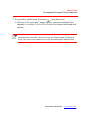
CHAPTER 6
Reviewing Data - View Results tab
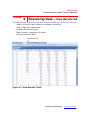
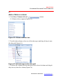
Add or Delete a Column ····································· 92
Sort or Filter the Column Data ······························ 94
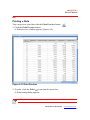
Exporting a Data··················································· 96
Printing a Data······················································ 98
CHAPTER 7
Data Charts – Create Graphs tab
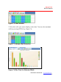
Viewing a Data Chart ········································· 99
Chart format ······················································· 104
Analyte Selector ················································· 105
Changing Color Palette ········································· 107
Changing Chart Properties ···································· 108
Printing a Chart ···················································· 109
®
MasterPlex
ReaderFit www.miraibio.com
II
Copying or Saving Chart Image ·························· 111
CHAPTER 8
Export Data – Customized Report Manager tab
Importing a User Defined Stylesheet ·················· 113
Exporting a User Defined Stylesheet ·················· 114
Delete Stylesheet File from Style Sheet List ········· 115
Including standard curve images ··························· 116
Transform Original Data into Your Customized
Data······································································ 116
APPENDIX A
Preferences
Grid Customize Menu ········································ 118
Print Preview Menu ············································ 125
APPENDIX B
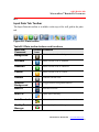
MasterPlex® ReaderFit Toolbars
Main File Menu and Toolbar ······························ 132
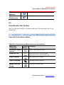
Input Data Tab Toolbar ······································ 134
View Results Tab Toolbar ·································· 135
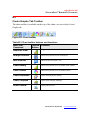
Create Graphs Tab Toolbar ································· 136
Customized Report Manager Tab Toolbar ·········· 137
APPENDIX C
Model Equations
Four Parameter Logistic Curve ··························· 138
Five Parameter Logistic Curve ···························· 139
Heteroscedasticity ·············································· 143
Weighted Nonlinear Least Square ······················· 149
Results of Weighting ·········································· 150
®
MasterPlex
ReaderFit www.miraibio.com
III
CHA PT E R 1
WELCOME
MiraiBio MasterPlex ReaderFit
®
CHAPTER
1
Welcome to the MiraiBio MasterPlex® ReaderFit User Manual. MasterPlex®
ReaderFit software analyzes results files (*.csv, *txt or *.xls) from the plate
reader instruments.
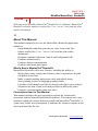
1.1
About This Manual
This manual explains how to use the MasterPlex® ReaderFit application
module to:
• Open blank plate and then paste the raw value from result files
• Import results files (*.csv, *.txt or *.xls) from the plate reader
instruments
• Designate standard, unknown, control, and background wells
• Generate standard curves
• Compute analyte concentrations
• Generate data charts and reports
What’s New in MasterPlex® ReaderFit
MasterPlex® ReaderFit offers new features, including the ability to:
• Merge plates using virtual plate feature so that it can analyzes beyond
100 panels at one time
• Make a sample marking and groups easily and quickly using
Auto-grouping feature or dragging grouping feature
• Calculate a fold change especially for being used relative gene analysis
• Normalize the data so that it can analyze between difference plates
• Generate a custom reports using style sheet
Conventions Used in This Manual
This manual describes the steps required to perform the various tasks
associated with the MasterPlex® ReaderFit software. The manual uses a step
format to explain the various tasks associated with MasterPlex® ReaderFit. A
symbol may follow a step instruction. It indicates the software response to the
action performed by the user.
®
MasterPlex
ReaderFit www.miraibio.com
1
CHA PT E R 1
WELCOME
Screen Captures
Screen captures may accompany the step instructions for further illustration.
The screen captures in this manual may not exactly match those displayed on
your screen.
1.2
Technical Support
You can contact MiraiBio Technical support at:
Hitachi Software Engineering America, Ltd.
601 Gateway Boulevard, Suite 100
South San Francisco, CA 94080
USA
Tel: +1 (650) 615-7600
Toll Free: +1 (888) 615-9600
Fax: +1 (650) 615-7639
E-mail: [email protected]
www.miraibio.com
®
MasterPlex
ReaderFit www.miraibio.com
2
CHA P T E R 2
INSTALLING MASTERPLEX® READERFIT
CHAPTER
2
Installing MasterPlex® ReaderFit
This chapter explains the minimum hardware and software requirements
needed to install and use MasterPlex® ReaderFit. It provides installation
instructions for a computer for your analysis.
2.1
Requirements
For optimum performance, MasterPlex® ReaderFit requires hardware and
software that meet or exceed the following specifications.
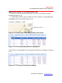
Minimum Hardware Requirements
Platform
CPU
Memory (RAM)
Storage space
(HDD)
Input devices
Video RAM
Monitor resolution
Monitor color
CD-ROM drive
PC
Intel Pentium 4 2 GHz or equivalent,
Intel Pentium 4 2 GHz or better (recommended)
512MB or higher for Windows XP/Vista/7
120 MB available hard drive space for the installation
Keyboard and mouse or other pointing device
32MB or higher
XGA (1024x768 pixels or higher; 1280 x1024
recommended)
16-bit color (high color) or higher
Required for CD media version. Not applicable for
download version.
Software Requirements
Operating system
Microsoft Windows XP/Vista/7,
Microsoft .NET3.5 framework required.
®
MasterPlex
ReaderFit www.miraibio.com
3
CHA P T E R 2
INSTALLING MASTERPLEX® READERFIT
2.2
Installing MasterPlex® ReaderFit
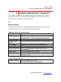
1. Insert the MasterPlex® CD-ROM in the workstation computer and
double-click setup.exe.
The installation begins and the InstallShield Wizard appears (Figure 2.1).
Figure 2.1 InstallShield Wizard, Welcome screen
2. To continue the installation, click Next.
The Customer Information window appears (Figure 2.2).
®
MasterPlex
ReaderFit www.miraibio.com
4
CHA P T E R 2
INSTALLING MASTERPLEX® READERFIT
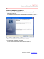
Figure 2.2 Customer Information screen
3. Input both User Name and Company Name, the click Next.
The Set Type window appears (Figure 2.3).
®
MasterPlex
ReaderFit www.miraibio.com
5
CHA P T E R 2
INSTALLING MASTERPLEX® READERFIT
4. Make sure the module name you purchased and click
want to install.
icon you don’t
Figure 2.4 Install module selection window
®
MasterPlex
ReaderFit www.miraibio.com
6
CHA P T E R 2
INSTALLING MASTERPLEX® READERFIT
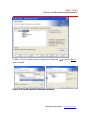
5. To continue, click Next.
The Ready to Install the Program window appears (Figure 2.5).
Figure 2.5 Ready to Install the Program window
6. Click Install.
The Start Copying Files window appears (Figure 2.6).
®
MasterPlex
ReaderFit www.miraibio.com
7
CHA P T E R 2
INSTALLING MASTERPLEX® READERFIT
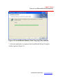
Figure 2.6 InstallShield Wizard, Start Copying Files window
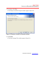
7. After the installation is completed, the InstallShield Wizard Complete
window appears (Figure 2.7).
®
MasterPlex
ReaderFit www.miraibio.com
8
CHA P T E R 2
INSTALLING MASTERPLEX® READERFIT
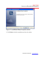
Figure 2.7 InstallShield Wizard Complete window
8. Click Finish to finish the installation and close the window.
®
MasterPlex
ReaderFit www.miraibio.com
9
CHA P T E R 2
INSTALLING MASTERPLEX® READERFIT
2.3
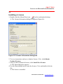
Installing a License
1. Double-click the MasterPlex® icon
on the workstation desktop.
The License Information dialog box appears (Figure 2.5).
Figure 2.5 License Information dialog box
2. To view instructions on how to obtain a license (*.lic), click Obtain
Product Licenses.
3. After you have obtained a license, click Install New License.
The Open dialog box appears.
4. Use the Open dialog box to locate the license (*.lic) and double-click the
file.
The license is installed.
®
MasterPlex
ReaderFit www.miraibio.com
10
CHA PT E R 3
GETTING STARTED
CHAPTER
3
Getting Started
This chapter provides a brief overview of data analysis using MasterPlex®
ReaderFit. It also explains how to start the software, import a result file
(.csv, .txt or .xls) from plate reader instruments, and the user interface
components.
3.1
Overview of MasterPlex® ReaderFit Analysis
MasterPlex® ReaderFit software analyzes results files (.csv, .txt or .xls) from
the major plate reader instruments. The analysis steps include:
• Import a results file (.csv, .txt or .xls)
• Designate well types (standard, unknown, background, or control) and
well groups (identify members of a standard data set or replicate
unknowns)
• Define the standard data set (enter standard concentrations and select a
model equation for the standard curve)
• Associate or link a standard data set to an unknown group(s)
• Compute the analyte concentrations
• Save the results file in MasterPlex® ReaderFit file format (.mxqs).
The .mxqs file includes information associated with the file (for example,
well definitions and interpolated concentrations)
After the concentrations are calculated, you can:
• View the results in graphs or several different report formats
• Create a virtual plate (a simulated microtiter plate) that contains data
from user-selected actual plates (.csv, .txt, or .xls)
®
MasterPlex
ReaderFit www.miraibio.com
11
CHA PT E R 3
GETTING STARTED
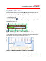
3.2
Starting MasterPlex® ReaderFit
On the desk top, double-click the MasterPlex® icon
. Alternatively, you
can click the Windows start menu button
and select Programs
> MasterPlex > MasterPlex.
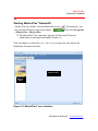
The MasterPlex® user interface appears and lists up all detected
applications in the application pane (Figure 3.1).
You can import a results file (.csv, .txt or .xls) or paste the raw data in the
blank plate from this interface.
Main window
Application
Module
Pane
Figure 3.1 MasterPlex® user interface
®
MasterPlex
ReaderFit www.miraibio.com
12
CHA PT E R 3
GETTING STARTED
3.3
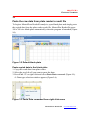
Paste the raw data from plate reader’s result file
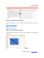
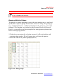
To begin a MasterPlex® ReaderFit analysis, open blank plate and simply paste
the copied date from the plate reader result file. MasterPlex ReaderFit opens
100 x 100 size blank plate automatically when the program is launched (Figure
3.2).
Figure 3.2 Default blank plate
Paste copied data in the blank plate
1. Copy the result data from plate reader.
2. Select the top left cell you want to paste the data
3. Press Ctrl + V or right click and select Paste Data command (Figure 3.3).
Data type selection window appears (Figure 3.4).
Figure 3.3 Paste Data command from right click menu
®
MasterPlex
ReaderFit www.miraibio.com
13
CHA PT E R 3
GETTING STARTED
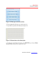
Figure 3.4 Data type selection window
4. Choose appropriate data type you want to paste in.
5. Copied data is pasted in the blank plate (Figure 3.5).
Figure 3.5 Pasted data in the blank plate
6. To delete the copied data in the plate, press DELETE key or choose Delete
Selected Wells command from right click menu.
®
MasterPlex
ReaderFit www.miraibio.com
14
CHA PT E R 3
GETTING STARTED
3.4
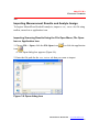
Importing Measurement Results and Analyte Assign
To begin a MasterPlex® ReaderFit analysis, import a .csv, .txt or .xls file using
toolbar, menu bar or application icon.
Importing Scanning Results Using the File Open Menu, File Open
Icon or Application Icon
1. Choose File > Open, click the File Open icon
or click the application
icon
.
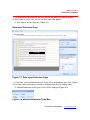
The Open dialog box appears (Figure 3.6).
2. Enter the file path for the .csv, .txt or .xls that you want to import.
Figure 3.6 Open dialog box
®
MasterPlex
ReaderFit www.miraibio.com
15
CHA PT E R 3
GETTING STARTED
3. Navigate to the directory of the .csv, .txt or .xls that you want to import.
4. Select one or more .csv, .txt or .xls files and click Open.
File import wizard appears (Figure 3.7).
Data Input Selection Page
Grid view
Figure 3.7 Data Input Selection Page
1. Select one of the deliminator type from select deliminator type box (Figure
3.8) so that your result data is correctly delimited in the file display grid.
Data delimitation in the grid view will be changed (Figure 3.9).
Figure 3.8 Select Deliminator Type Box
®
MasterPlex
ReaderFit www.miraibio.com
16
CHA PT E R 3
GETTING STARTED
Figure 3.9 Data Delimitation Change
2. Select data format type from select data format box (Figure 3.10), plate or
list.
Figure 3.10 Select Data Format Box
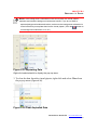
3. (In case of Plate) Select data area you want to import by mouse dragging
(Figure 3.11).
Figure 3.11 Data selection by mouse dragging
®
MasterPlex
ReaderFit www.miraibio.com
17
CHA PT E R 3
GETTING STARTED
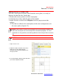
4-1. (In case of List) First select well address by mouse dragging, then click
Done button for well address column (Figure 3.12).
Column next to the well address is automatically selected(Figure 3.13).
Figure 3.12 Well Address Selection
Figure 3.13 Auto Intensity Data Selection
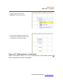
4-2. (In case of List) Next, select intensity data by mouse dragging, then click
done button for intensity column. If auto selected column is the intensity data
column, just click done button for intensity column (Figure 3.14).
Figure 3.14 Click Done Button for Intensity Column
®
MasterPlex
ReaderFit www.miraibio.com
18
CHA PT E R 3
GETTING STARTED
5. Click Next to proceed (Figure 3.15).
Figure 3.15 Next Button
®
MasterPlex
ReaderFit www.miraibio.com
19
CHA PT E R 3
GETTING STARTED
Analyte Assignement Page
Analyte mode selection
Available Analytes list
Mini plate preview
Remove analyte button
Figure 3.16 Analyte Assignment Page
1. Select wells for the analyte your are trying to specify.
2. Click Assign button
Selected wells are registered as an analyte, and listed in the Available
Analytes list. (Figure 3.17)
3. Rename the analyte name or the color if you want. (default analyte name is
‘Analte n’, color is randam) (Figure 3.18)
4. Repeat analyte assignment. (Figure 3.19)
5. When all wells were assigned, click OK.
Analyte assignment dialog closes and plate is build on plate view. (Figure
3.20)
®
MasterPlex
ReaderFit www.miraibio.com
20
CHA PT E R 3
GETTING STARTED
Figure 3.3 Analyte Assign dialog
Figure 3.17 Data Selection
Figure 3.18 Data Assignment
®
MasterPlex
ReaderFit www.miraibio.com
21
CHA PT E R 3
GETTING STARTED
Figure 3.19 Naming and Color Change
Figure 3.20 Analyte Assign dialog
®
MasterPlex
ReaderFit www.miraibio.com
22
CHA PT E R 3
GETTING STARTED
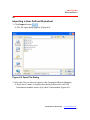
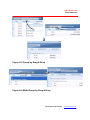
3.5
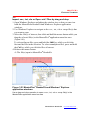
Import .csv, .txt, .xls or Open .mlx* Files by drag and drop
1. Open Windows Explorer and adjust the window size so that you can view
both the MasterPlex® ReaderFit and Windows® Explorer application
windows.
2. Use Windows Explorer to navigate to the .csv, .txt, .xls or .mxqs file(s) that
you want to open.
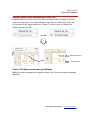
3. Select the file(s) of interest, then click and hold the mouse button while you
drag the selected file(s) to the MasterPlex® application menu bar area
(Figure 3.21).
To select adjacent files, press and hold the Shift key while you click the
first and last file in the selection. To select nonadjacent files, press and hold
the Ctrl key while you click the files of interest.
4. Release the mouse button.
The file(s) open in MasterPlex® ReaderFit.
Figure 3.21 MasterPlex® ReaderFit and Windows® Explorer
application windows
Use a drag-and-drop operation to open a .csv, .txt, .xls or .mxqs file(s) in the
MasterPlex® application menu bar area
®
MasterPlex
ReaderFit www.miraibio.com
23
CHA PT E R 3
GETTING STARTED
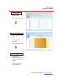
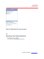
3.6
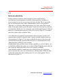
Tab categorized work flow
ReaderFit application module consists of five tab pages, Input Data, Fit
Curves, View Results, Create Graphs and Customized Report Manager
(Figure 3.22), designed to match the work flow in a typical multiplex data
analysis session.
Figure 3.22 ReaderFit application module tabs
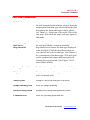
Define a Plate
-
Mark sample as
Background, Standard,
Unknown or Control
-
Fill out standard value
Draw Standard Curve
-
Choose a model
equation, and set
options
-
Review regression
curve and data
-
Make some outliers and
re-calculate the curve
®
MasterPlex
ReaderFit www.miraibio.com
24
CHA PT E R 3
GETTING STARTED
Review Data
-
Review all data
-
Print or export the data
Review Data by Chart
-
Review all data on the
chart
-
Customize chart
properties
-
Print or export the chart
Export Customized Data
-
Transform the
MasterPlexReaderFit
xml data to original data
format
-
Import or export the
style sheet data
®
MasterPlex
ReaderFit www.miraibio.com
25
CHA PT E R 3
GETTING STARTED
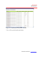
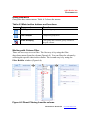
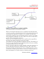
3.7
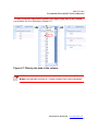
Viewing Data in the Input Data Tab
The ReaderFit application module starts in the Input Data tab. If any other tab
page is displayed, click the Input Data tab to display the Input Data tab as
shown below(Figure 3.23).
Input Data tab
Figure 3.23 Input Data tab page
1. If more than one application window is open, select the Cascade,
Tile Horizontal , or
Tile Vertical menu from the window menu bar
to arrange the application windows for easier viewing.
2. To change the data displayed in the well grid:
a. Click an analyte in the Analyte pane.
b. Make a selection from the data type upper drop-down list.
The well grid displays the data for the selected analyte.
Figure 3.24 shows the components of the Input Data tab. Table 3.1 lists the
®
MasterPlex
ReaderFit www.miraibio.com
26
CHA PT E R 3
GETTING STARTED
types of data available for display in the plate view.
3. To view background-subtracted data, click the Subtract background
button
.
The Input Data tab displays background-subtracted data.
For more information on background calculation options, see Background
Type on section 4.6.
Data type ‘upper’ and ‘lower’ drop-down list
Lower grid switch
Display box
Subtract Background button
Sample marking icon
Command icon
Analyte Pane
Well grid
Figure 3.24 Input Data tab and Analyte pane
®
MasterPlex
ReaderFit www.miraibio.com
27
CHA PT E R 3
GETTING STARTED
Plate View Components
Well Grid
A representation of a microtiter plate that displays
the well contents for the analyte selected from the
analyte panel and data type selected from the data
drop-down list. Some data types can be edited
(see Table 3.1). Select one of the wells (The wells
turn gray), then click the same well once again to
edit mode.
Data type ‘upper’
and ‘lower’
drop-down list
Shows the types of data available for display in
the well grid. Make a selection from this
drop-down list to choose the data type displayed
in the well grid. Click the drop-down arrow to
view the list and select a data type. (See Table 3.1
for a description of the data types.) The well grid
can be separated into upper and lower grids by
clicking lower grid switch. (See Figure 3.8 for
more further details)
Lower grid switch
Enables the lower grid data selection and display.
Display box
Displays the selected data type value for the
active (selected) well.
Analyte pane
Displays a list of the analytes in an assay.
Sample marking icon
Icons for sample marking.
Subtract background
Displays the background-subtracted value.
Command icon
Icons for operating input data tab.
®
MasterPlex
ReaderFit www.miraibio.com
28
CHA PT E R 3
GETTING STARTED
Table 3.1 Data Types in the well grid
Data Type
Description
Edit
Data
Response Values
Calculated Values
Independent Values
Standard Links
Outlier Status
Sample Name
Replicate Group
Name
Analyte Name
Dilution Factor
Response Mean
Response SD
Response %CV
Calculated Mean
Calculated SD
Calculated %CV
Intensity
The luminescence intensity measured by the
plate reader instruments.
The analyte concentration that is computed
(interpolated or extrapolated) from the
user-selected standard curve.
The dilution factor for the well.
Shows the standard number that is linked to
each well or well group.
A check mark indicates the well is outlier and
the well data are not included in the calculation
of concentrations.
User-specified name for the well.
The group name of the well. Wells that belong
to the same group have the same group
number.
The analyte name assigned to the well. Wells
that belong to the same group have the same
group number.
The dilution factor for the well.
Shows the Response Value average within the
group.
Shows the Response Value standard deviation
within the group.
Shows the Response Value %CV within the
group.
Shows the concentration average within the
group.
Shows the concentration standard deviation
within the group.
Shows the concentration %CV within the group.
Shows the Normalized data within the group.
(This data type is available in the lower dropdown list only.)
®
MasterPlex
No
No
Yes
Yes
Yes
Yes
Yes
Yes
Yes
No
No
No
No
No
No
No
ReaderFit www.miraibio.com
29
CHA PT E R 3
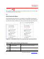
GETTING STARTED
Display Double Data Information in one Cell
ReaderFit has an unique feature for data viewing on the well grid. You can
select two data type from various kind of data, and it is displayed in the one
cell separated into upper and lower. Figure 3.8 shows how to display the
double data in one cell.
Response Values
Analyte Name
Figure 3.25 Upper and lower grid display
Well grid can be separated into upper and lower grid. Each grid displays separate
data type.
®
MasterPlex
ReaderFit www.miraibio.com
30
CHA PT E R 3
GETTING STARTED
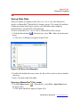
3.8
Saving Plate Data
After you import a scanning results file (.csv, .txt or .xls), the data can be
saved to a MasterPlex® ReaderFit file format (.mxqs). The .mxqs file includes
all data associated with a plate such as well definitions and computed
(interpolated or extrapolated) concentrations.
To save results data (.csv, .txt or .xls) to a MasterPlex® file (.mxqs):
1. Click the Save button
. Alternatively, select File > Save from the main
menu.
The Save As dialog box appears (Figure 3.26).
Figure 3.26 Save As dialog box
2. Confirm the default directory where the file will be saved or choose another
directory.
3. Enter a file name and click Save.
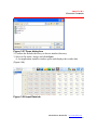
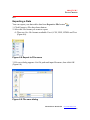
Opening a MasterPlex® File (.mxqs)
1. Click the Open button
. Alternatively, select File > Open Plate from
the main menu.
The Open dialog box appears (Figure 3.27).
®
MasterPlex
ReaderFit www.miraibio.com
31
CHA PT E R 3
GETTING STARTED
Figure 3.27 Open dialog box
2. Confirm the default directory or choose another directory.
3. Select a file name (.mxqs) and click Open.
An application module window opens and displays the results data
(Figure 3.28).
Figure 3.28 Input Data tab
®
MasterPlex
ReaderFit www.miraibio.com
32
CHA PT E R 4
DEFINING A PLATE
CHAPTER
4
Defining a Plate – Input Data tab
After you import a scanning results file (.csv, .txt or .xls), your analysis begins
by defining a plate. This chapter explains how to define and save a plate. The
steps to define a plate include:
• Designate well type to identify the standard, unknown, background,
and control wells.
• Create a standard data set(s) by entering the concentration for each
well in the standard data set. A plate can have more than one standard
data set.
• Link each well group to a standard data set to specify the standard
that is used to compute (interpolate or extrapolate) the analyte
concentrations.
The plate definition can be saved as a template that can be applied to other
plates. The Template Manager helps you manage your templates. For more
information on templates, see Working With Templates (on section 4.5).
4.1
Designating Well Type and Group
Selecting Wells
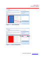
To select a well in the Input Data tab, click the well in the well grid. There are
three ways to select multiple wells:
• To select adjacent wells (Figure 4.1), press and hold the mouse button
while you drag the pointer over the wells that you want to select. Click
and release the mouse button to select the highlighted wells.
• To select adjacent wells, press and hold the Shift key while you click
the first and last well in the selection.
• To select nonadjacent wells (Figure 4.2), press and hold the Ctrl while
you click the wells.
®
MasterPlex
ReaderFit www.miraibio.com
33
CHA PT E R 4
DEFINING A PLATE
Figure 4.1 Well grid selection
To select adjacent wells, press and hold the Shift key while you click the first and
last well in the selection. Alternatively, press and hold the mouse button while you
drag the mouse over the wells of interest.
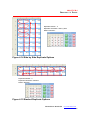
Figure 4.2 Well grid random selection
To select nonadjacent wells, press and hold the Ctrl key while you click the wells of
interest.
®
MasterPlex
ReaderFit www.miraibio.com
34
CHA PT E R 4
DEFINING A PLATE
Designating Well Type
Table 4.1 shows the types of wells that are available.
1. Select the well(s) that you want to define.
2. To define (or mark) the well(s), click one of the icons located on the upper
well grid (Figure 4.3). You can also right-click the selection and choose a
well type from the pop-up menu that appears Figure 4.4. (Table 4.1).
The well type is applied to the selected well(s).
Figure 4.3 Sample mark icons
Figure 4.4 Well grid pop-up menu
Right click a well to display the pop-up menu
®
MasterPlex
ReaderFit www.miraibio.com
35
CHA PT E R 4
DEFINING A PLATE
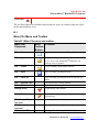
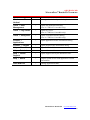
Table 4.1 Sample mark icon and context menu to define wells
Well Type
Button Context menu on the well
grid
Background
Background
Wells that contain no analytes.
Standard
Standard
Wells that contains analyte of known
concentration.
Unknown
Unknown
Wells that contains analytes of unknown
concentration.
Control
Control
Wells that contain analytes that function as
controls for a particular assay design.
Unmark
Unmark
Clear the current marking.
If a well belongs to a group, unmarking the well also removes the
well from the group.
3. Repeat step 1 and step 2 to mark and group other well(s).
Designating Well Groups
After you have defined the wells, the wells are organized into groups
automatically so that the software can identify:
• Replicate unknowns
• A standard data set
MasterPlex® ReaderFit automatically places all background wells into one
group. You can define one or more groups of control wells per plate.
®
MasterPlex
ReaderFit www.miraibio.com
36
CHA PT E R 4
DEFINING A PLATE
NOTE: A group can include nonadjacent wells. A plate can have more than one
group of standards or unknowns.
Grouping Wells by Pattern
The purpose of pattern grouping is to provide users another way to easily and
quickly make replicate groups. Pattern here means two things: the group type
(e.g., standard, unknown…) and the dimensions of the group (i.e., rows and
columns). This function acts similarly to the Resizing feature of Microsoft
Excel. It is especially useful when the plate has many groups/replicates that
follow similar group patterns.
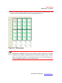
1. Define the group pattern by selecting a group of wells, and marking and
grouping them together. We will group other wells into this pattern.
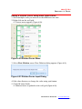
2. Select all wells of the pattern group(Figure 4.5).
Figure 4.5 Well groups
®
MasterPlex
ReaderFit www.miraibio.com
37
CHA PT E R 4
DEFINING A PLATE
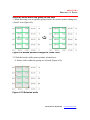
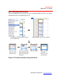
3. Move the pointer to the bottom-right corner of the selection. When you see
the pointer turn into a black cross, hold down the left mouse button and drag
the pointer over the selection. During dragging, you will see in real-time that
new wells are selected and grouped into the pattern, as indicated by a red-line
border (Figure 4.6).
Figure 4.6 Making Well groups by mouse Dragging
®
MasterPlex
ReaderFit www.miraibio.com
38
CHA PT E R 4
DEFINING A PLATE
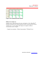
4. Once you are satisfied with the selection, just release the mouse button. The
software will automatically finish the grouping(Figure 4.7).
Figure 4.7 Well groups
NOTE: When starting drag, you can move the pointer, you can move it either
downwards or rightwards, which results in different ways to select wells. To switch
between the two modes, just drag the pointer back into the pattern group, and then
drag it out in either direction. So, it is determined by your first move direction when
you are dragging the pointer out of the pattern group.
®
MasterPlex
ReaderFit www.miraibio.com
39
CHA PT E R 4
DEFINING A PLATE
Figure 4.8 Making Well groups by mouse Dragging
Dragging downwards as the first move (above) vs. dragging rightwards as the first
move (below)
®
MasterPlex
ReaderFit www.miraibio.com
40
CHA PT E R 4
DEFINING A PLATE
Select all wells within the group at one time
1. While hovering over a replicate group border, the mouse pointer changes to
a ‘hand’ icon (Figure 4.9).
Figure 4.9 Mouse pointer changes to ‘hand’ icon
2. Click the border while mouse pointer is hand icon.
Entire wells within the group are selected (Figure 4.10).
Figure 4.10 Selected wells
®
MasterPlex
ReaderFit www.miraibio.com
41
CHA PT E R 4
DEFINING A PLATE
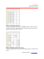
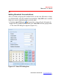
4.2
Setting Standard Concentrations
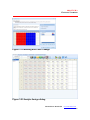
After you define and group the standard wells, use the auto fill feature to help
you automatically enter the standard concentrations. Auto-Fill icon is enabled
when one or more standard groups are in the plate.
1. Click the Auto-Fill button
located above the well grid. Alternatively,
Right-click the standard data set and select Auto-Fill from the popup menu.
The Auto Fill dialog box appears (Figure 4.11).
Figure 4.11 Auto Fill dialog box
®
MasterPlex
ReaderFit www.miraibio.com
42
CHA PT E R 4
DEFINING A PLATE
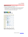
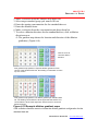
2. Make a selection from the Analyte drop-down list.
3. Select target standard group you want to fill out.
4. Enter the starting concentration for the standard data set.
5. Enter the dilution factor.
6. Make a selection from the concentration unit drop-down list
7. To select a dilution direction for the standard data set, click a dilution
direction arrow.
The gradient map shows the location and direction of the dilution
gradient(s) (Figure 4.12).
Click an arrow to
choose a dilution
direction.
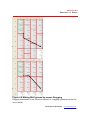
This gradient map specifies a separate dilution gradient in each
column of the standard data set. The starting concentration is at the
top of a column.
This gradient map specifies one dilution gradient per standard data
set. The starting concentration is at the upper left well and the end
concentration is at the lower right well. Click an arrow to choose a
dilution direction.
Figure 4.12 Example dilution gradient maps
Click a dilution direction arrow to choose the dilution gradient configuration for the
standard data set.
®
MasterPlex
ReaderFit www.miraibio.com
43
CHA PT E R 4
DEFINING A PLATE
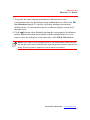
7. To specify the same starting concentration, dilution factor, and
concentration units for all analytes in the standard data set, choose the Fill
for all analytes option. To specify a different starting concentration,
dilution factor, or concentration unit for a different analyte, repeat step 2
through step 4.
8. Click Apply button when finished entering the concentration, the dilution,
and the dilution direction for all analytes in the standard data set. If you
want to close the dialog box at the same time, click Fill & Close button.
NOTE: If you want to fill the standard value for your desired wells, select wells on
the well grid, and choose ‘Selected Wells’ at the target well selection in the Auto-Fill
dialog. Auto-Fill process is applied for only the wells you selected.
®
MasterPlex
ReaderFit www.miraibio.com
44
CHA PT E R 4
DEFINING A PLATE
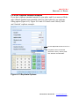
Fill in for replicate standard samples
If you have replicate standard samples in your plate, and if you want to fill the
same diluted standard concentration value for each replicates, use replicate
filling option (Figure 4.13). Figure 4.14 and 4.15 shows each ‘Side by Side’
and ‘Stacked’ replicate example.
Choose Replicate Number from 2 to 5
If replicate number is selected
(other than ‘None’), ‘Side by Side’
and ‘Stacked’ are selectable..
Figure 4.13 Replicate Options
®
MasterPlex
ReaderFit www.miraibio.com
45
CHA PT E R 4
DEFINING A PLATE
Replicate Number : 2
Replicate Orientation: Side by Side
Dilution Direction:
Figure 4.14 Side by Side Replicate Options
Replicate Number : 3
Replicate Orientation: Stacked
Dilution Direction:
Figure 4.15 Stacked Replicate Options
®
MasterPlex
ReaderFit www.miraibio.com
46
CHA PT E R 4
DEFINING A PLATE
Input Standard Data Manually
If your standard data series does not have sequential diluted values, use direct
edit mode on the well grid(Figure 4.16) .
Set data type as standard in the upper or
lower dropdown list.
Click one of the
well you want to
input the value.
Click same well again,
press character key or
press F2 to enter the
edit mode.
Standard data is shown in the well grid.
Input the value.
Click other well,
enter key or
ESC key to exit
the edit mode.
Figure 4.16 Input manually using edit mode
®
MasterPlex
ReaderFit www.miraibio.com
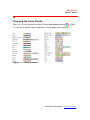
47
CHA PT E R 4
DEFINING A PLATE
4.3
Linking a Standard Data Set
Background, control, and unknown wells must be associated with or linked to
the standard data set that will be used to calculate concentrations. By default,
the first standard that you define will be linked to the background, control, and
unknown well groups.
If there is more than one standard on the plate, you can link a user-selected
standard to a user-selected well group(s).
1. To link a well group to a standard data set, press and hold the Ctrl key
while you click the group and the standard data set that you want to link.
NOTE: A standard data set can be linked to multiple groups of the same well type,
but each group can have only one standard.
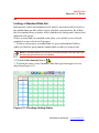
2. Click the Link Standard button
.
3. To check the status, select Standard Links data type from upper or lower
drop-down(Figure 4.17).
Figure 4.17 Checking Linking Status
®
MasterPlex
ReaderFit www.miraibio.com
48
CHA PT E R 4
DEFINING A PLATE
4.4
Working With Diluted Unknowns
If you need to dilute a sample prior to an assay, you can specify a dilution
factor in the well grid. MasterPlex® ReaderFit can compute the diluted analyte
concentration.
For a diluted unknown:
Original concentration = Dilution factor * Calculated concentration.
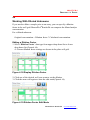
Editing a Dilution Factor
1. Select ‘Dilution Factor’ data type from upper drop-down list or lower
drop-down list (Figure 4.18).
Current dilution factor settings are shown in the plate well grid.
Figure 4.18 Display Dilution Factor
2. Click one of the desired well your want to set the dilution.
3. Click the same well again to enter the edit mode(Figure 4.19).
Figure 4.19 Dilution Factor Edit Mode
®
MasterPlex
ReaderFit www.miraibio.com
49
CHA PT E R 4
DEFINING A PLATE
Editing a Dilution Factor using batch input feature
1. Select multiple wells you want to set the dilution at one time.
2. Right click on the well grid.
Context menu appears (Figure 4.20).
Figure 4.20 Dilution Factor Menu
3. Select Plate Dilution menu. Plate Dilution dialog appears (Figure 4.21).
Figure 4.21 Dilution Factor Input Dialog
4. Edit value directory or change the value using spin button.
5. Click OK when finish.
Dilution factor is updated on the well grid (Figure 4.22).
®
MasterPlex
ReaderFit www.miraibio.com
50
CHA PT E R 4
DEFINING A PLATE
Figure 4.22 Inputted Dilution Factor
Dilution for Unknowns
Samples can be diluted prior to the assay and analysis. After MasterPlex®
ReaderFit interpolates the diluted unknown analyte concentrations from the
standard curve, it can compute and display the original, undiluted
concentration in the well grid.
Original concentration = Diluted concentration * Dilution Factor
®
MasterPlex
ReaderFit www.miraibio.com
51
CHA PT E R 4
DEFINING A PLATE
4.5
Working With Templates
A plate definition includes:
• Well types and well groups
• Standards (including standard concentrations, associated model equation,
and concentration units)
• Links between the standard(s) and well groups
• Data calculated for the plate (for example, analyte concentrations or
standard data curves)
• Data manually entered in the plate (for example, sample names or
dilution factors)
You can save the plate definition as a template. You can apply a template to
an active plate. Templates may also be exported, imported, or deleted.
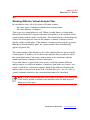
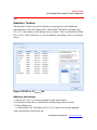
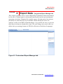
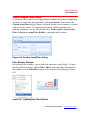
Opening the Template Manager
The Template Manager is a tool that helps you manage your templates.
1. Click the Template Manager button
.
The Template Manager appears (Figure 4.23).
2. Click a template in the Available Templates list to view information about
the template.
Figure 4.23 Template Manager shows available templates
®
MasterPlex
ReaderFit www.miraibio.com
52
CHA PT E R 4
DEFINING A PLATE
Click a template to view information about the template.
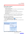
Saving a Template
You can save the current plate definition to a template.
1. After you have finished defining a plate, open the Template Manager and
click the Save button.
The Template Name and Description box appears (Figure 4.24).
Figure 4.24 Template Name and Description box
2. Enter a name and descriptions for the template and click OK.
The new template is added to the Available Template list.
Loading a Template
You can apply or load a saved template to the current plate.
1. In the Template Manager, select the template that you want to apply to the
plate.
2. Click the Load button.
The template is applied and the well grid shows the new well attributes
(well type, well group, and links to standard data sets).
Overwriting a Template
You can overwrite an existing template with the current plate definition.
1. In the Template Manager, select the template that you want to overwrite
2. Click the Overwrite button.
A confirmation box appears (Figure 4.25).
®
MasterPlex
ReaderFit www.miraibio.com
53
CHA PT E R 4
DEFINING A PLATE
Figure 4.25 Confirmation box
1. Click OK to overwrite the selected template with the current plate
definition.
Exporting a Template
You can export a template to a user-specified location.
1. In the Template Manager, click the template you want to export.
2. Click the Export button.
The Save As dialog box appears (Figure 4.26).
Figure 4.26 Save As dialog box
3. Choose the directory for the template that you want to export.
®
MasterPlex
ReaderFit www.miraibio.com
54
CHA PT E R 4
DEFINING A PLATE
4. Enter a name for the template (*.mxtq).
NOTE: A template must have a .mxtq file extension. Changing the extension will
render the exported template unusable.
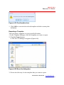
Importing a Template
You can import a template (.mxtq) from a user-specified location.
1. In the Template Manager, click Import button.
The Open dialog box appears (Figure 4.27).
Figure 4.27 Open dialog box
2. Choose the directory with the template that you want to import.
3. Select the template and click Open.
The template name is added to the Template Manager.
Deleting a Template
You can delete a template (.mxtq) from the system.
1. In the Template Manager, click the template that you want to delete.
2. Click Delete button.
®
MasterPlex
ReaderFit www.miraibio.com
55
CHA PT E R 4
DEFINING A PLATE
A confirmation box appears (Figure 4.28).
Figure 4.28 Confirmation box
3. Click OK to delete the template.
The template is removed from the Template Manager.
WARNING: This permanently removes the template from the system.
®
MasterPlex
ReaderFit www.miraibio.com
56
CHA PT E R 4
DEFINING A PLATE
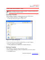
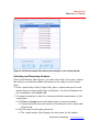
4.6
Preferences
Preferences are user-modifiable software settings. They are displayed in the
Preferences dialog box.
• To open the Preferences dialog box (Figure 4.29), click the Preferences
button
.
Figure 4.29 Preferences dialog box
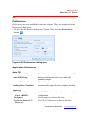
Application Preferences
Auto Fill
Automatically Popup
Auto Fill Dialog
Auto-calculate after
loading Plate Template
Best Fit
Root Mean Square
Error (RMSE)
R-Square
Least deviation of %
Recovery
Check this option if you want to open autofill
dialog automatically when you mark the
standard sample.
Check this option if you want to calculate
automatically right after the template loading.
Use RMSE index to choose the best curve fit
combination.
Use R-square to choose the best.
Use LD of % Recover to choose the best.
®
MasterPlex
ReaderFit www.miraibio.com
57
CHA PT E R 4
DEFINING A PLATE
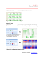
Split Cell Color
Color lower grid by specified color.
Figure 4.30 Colored lower well grid
Intensity Color
One Color
Two Color
Use one color for representing the value shading.
Use two colors for representing the value shading.
Click ‘one color’ and select desired color for
the maximum value. The color density
decreases directly with the value.
Click ‘two colors’ and select desired color for the
maximum and minimum value. The color shifts
upper to lower directly with the value.
Figure 4.32 Example of Intensity color
®
MasterPlex
ReaderFit www.miraibio.com
58
CHA PT E R 4
DEFINING A PLATE
Plate Preferences
Plate Information
Original File Name
Analyst Name
Plate Name
Background type
Average
Peak Value
Lowest Value
Displays the name assigned to the result file in
the plate reader software. To edit the plate name,
enter a new name.
Displays the analyst name entered in the plate
reader.
Shows plate name of this file.
Calculate average value in the background group.
Background (Bkg) Response Value = (Bkg
Response Value1 + Bkg Response Value2 +... Bkg
Response Valuen)/n
where n = the number of background wells in the
plate
Take highest value in the background group.
Take lowest value in the background group.
®
MasterPlex
ReaderFit www.miraibio.com
59
CHA PT E R 4
DEFINING A PLATE
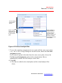
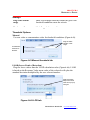
Threshold
You can select one of the criteria for threshold marker from Response Value,
Concentration and Error range. Select one of them and enter a Response Value,
concentration or error range threshold for a plate. The software automatically
marks wells that contain data less than the user specified threshold with a red
border (Figure 4.18).
To set a threshold(s):
1. Check ‘Show threshold marker’ box
2. Check one of the radio button in front of the data type you want to use as a
threshold marker.
3. Select equity equal symbol and input the value in the box.
4. Click Apply to reflect current setting to the plate, or click OK to reflect and
close the dialog box.
A red border marks wells that contain data less than or greater than
threshold for all analyte (Figure 4.28).
Figure 4.31 Well grid
Outlier Options
Show threshold
Marker
Response Value
Show red rectangle indicator inside the grid if the
threshold conditions meet the criteria.
Use Response Value for threshold conditions.
®
MasterPlex
ReaderFit www.miraibio.com
60
CHA PT E R 4
DEFINING A PLATE
Concentration
Use Concentration value for threshold conditions.
Error Range
Use Error Range for threshold conditions.
Automatic outliers
Automatically check on/off the outlier check box
for the wells. To check on, click Set button. To
check off, click Clear button.
®
MasterPlex
ReaderFit www.miraibio.com
61
CHA PT E R 4
DEFINING A PLATE
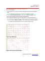
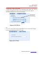
4.7
Creating a Virtual Plate
1. Open the measured results files (.csv, .txt or .xls) or MasterPlex® ReaderFit
files (.mlx*) that are the data sources for the virtual plate.
2. Click the Virtual Plate button .
The Virtual Plate dialog appears (Figure 4.33).
Figure 4.33 Plate Wizard, Plate Dimensions tab
3. Enter the number of rows and columns for the virtual plate. Click OK.
A module window opens and displays the empty well grid of the
virtual plate (Figure 4.34).
®
MasterPlex
ReaderFit www.miraibio.com
62
CHA PT E R 4
DEFINING A PLATE
Figure 4.34 Virtual plate
Selecting Data from a Source Plate
The virtual pipette copies (aspirates) data from user-selected wells in a source
plate and pastes (dispenses) the data into a virtual plate. The virtual pipette
copies all of the analyte data in a well, including the computed analyte
concentrations. It remains loaded until you dispense or clear the pipette.
NOTE: The data source plates must contain the same type and number of analytes,
otherwise concentrations cannot be calculated. If the source plates contain the
same number of analytes, but they are named differently, use the virtual analyte
filter to rename analytes so that the nomenclature is consistent. (See Working with
the Virtual Analyte Filter on section 4.8.)
1. In the source plate, select the wells of interest.
To select adjacent wells, press and hold the mouse button while you drag
the mouse pointer to select the wells of interest.
NOTE: Selecting non-adjacent wells is not recommended.
2. Right-click the selected wells and select Aspirate from the pop-up menu
that appears (Figure 4.35).
The data for the analytes in the selected wells are added to the virtual
pipette and is ready to dispense into a virtual plate.
®
MasterPlex
ReaderFit www.miraibio.com
63
CHA PT E R 4
DEFINING A PLATE
NOTE: If the background is subtracted in the source plate, the virtual pipette
aspirates and transfers background-subtracted values. If you do not want to
aspirate background-subtracted values, make sure the background subtraction is
turned off before you aspirate data into the virtual pipette. (Click the
button to
turn background subtraction on or off.)
Figure 4.35 Aspirating Data
Right-click selected wells to display the pop-up menu.
3. To clear the data from the virtual pipette, right-click and select Clear from
the pop-up menu (Figure 4.36).
Figure 4.36 Clear Aspirated Data
®
MasterPlex
ReaderFit www.miraibio.com
64
CHA PT E R 4
DEFINING A PLATE
Adding Data to a Virtual Plate
After the virtual pipette aspirates data from the source plate, it is ready to
dispense the data into the virtual plate.
1. Position the mouse pointer over the virtual plate.
2. Click the first well to which the data will be added.
3. Right-click the well and select Dispense from the pop-up menu that
appears.
The data are added to the virtual plate (in the same configuration as in
the source plate) (Figure 4.37).
NOTE: If the number or names of the analytes in the virtual pipette is different from
that in the virtual plate, the virtual analyte filter automatically appears. For more
information on using the filter, see Working With the Virtual Analyte Filter on section
4.9.
NOTE: Data in a virtual plate cannot be removed, but can be overwritten.
1. Open a .mlx or .csv.
2. Select the wells of interest in the source
plate (.csv or .mlx). Right-click the
selected wells and choose aspirate from
the pop-up menu.
3. In the virtual plate, select the first well where
you want to dispense the data.
®
MasterPlex
ReaderFit www.miraibio.com
65
CHA PT E R 4
DEFINING A PLATE
4. Right-click the well and select
Dispense from the pop-up menu.
5. The data are added to the virtual plate
(starting at the selected well) in the same
configuration as in the source plate.
Figure 4.37 Adding data to a virtual plate
Open a source plate (.mlx or .csv, .txt or .xls) and create a virtual plate (click the
button to generate the blank virtual plate).
®
MasterPlex
ReaderFit www.miraibio.com
66
CHA PT E R 4
DEFINING A PLATE
4.8
Working With the Virtual Analyte Filter
In a multiplex assay, all of the plate wells must contain:
• The same types of analytes with the same nomenclature
• The same number of analytes
This is true for virtual plates as well. When you add data to a virtual plate,
MasterPlex® ReaderFit compares the name and number of the analytes in the
virtual pipette to those in the virtual plate. The virtual pipette will not dispense
if there are discrepancies between the number or names of analytes in the
pipette and the virtual plate. If the number of analytes in the pipette is greater
than that of the destination plate, the virtual analyte filter automatically
appears (Figure 4.38).
The virtual analyte filter displays a list of the analytes that are present in the
virtual pipette. It enables you to choose the analytes that you want to add to
the virtual plate and, if necessary, rename them to be consistent with the
number and name of analytes in the virtual plate.
If you add data to a virtual plate from source wells that contain different
analyte names or a different number of analytes, data holes are created. As a
result, a well in the virtual plate appears blank if the analyte selected in the
analyte panel is not present in the well. If a plate file (.csv, .txt, xls, .mlx, or
virtual) contains data holes, the concentrations cannot be calculated.
NOTE: In order to prevent data holes, if the number of analytes in the virtual pipette
is less than the number of analytes in the destination plate, the data cannot be
added to the virtual plate.
®
MasterPlex
ReaderFit www.miraibio.com
67
CHA PT E R 4
DEFINING A PLATE
Figure 4.38 Virtual analyte filter shows the analytes in the virtual pipette
Selecting and Renaming Analytes
If the virtual analyte filter appears, you must select and, if necessary, rename
the analytes to match the number and names of the analytes in the virtual
plate.
1. In the virtual analyte filter (Figure 4.38), place a check mark next to each
analyte that you want to add to the virtual plate. To select all analytes for
the virtual plate, click Check All.
2. To rename an analyte so that it is consistent with the nomenclature in the
virtual plate:
a. Click here to assign next to the analyte that you want to rename.
A drop-down list shows the names of the analytes in the virtual plate
(Figure 4.39).
b. Select a name from the drop-down list.
The virtual analyte filter displays the new name for the analyte.
®
MasterPlex
ReaderFit www.miraibio.com
68
CHA PT E R 4
DEFINING A PLATE
List of analytes
in the virtual
pipette.
Click to display a
drop-down list of
analyte names in
the virtual plate.
Select a name from
the list to rename
the analyte from the
source plate.
Place a check
mark next to an
analyte to add
it to the virtual
plate.
Figure 4.39 Virtual analyte filter
3. To save the renaming assignments for use again with the same source plate
(.csv, .txt or .xls or .mxqs) during the current session, choose the Save this
assignment option.
If you want to aspirate other data from the same source plate, choose the
Use last saved assignments option in the virtual analyte filter to
automatically rename all of the analytes in the filter.
4. Click OK.
The data are added to the virtual plate and the virtual analyte filter
closes.
®
MasterPlex
ReaderFit www.miraibio.com
69
CHA PT E R 4
DEFINING A PLATE
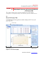
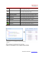
4. 9
Quality Control Manager
Quality Control Manager helps you flag and optionally set as an outlier any
wells whose value is outside of the range defined by the thresholds.
Thresholds can be assigned using the manual method for
- A single selected analyte
- Multiple selected analytes
- All analytes
• To open the Quality Control Manager (Figure 4.40), click the Quality
Control Manager button
.
Figure 4.40 Quality Control Manager dialog
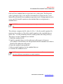
The software automatically marks wells that contain data less than the user
®
MasterPlex
ReaderFit www.miraibio.com
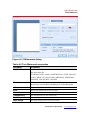
70
CHA PT E R 4
DEFINING A PLATE
specified threshold with a red border (Figure 4.41).
To set a threshold(s):
1. Select analytes you want to attach the threshold criteria from the analyte
pane.
Use All analytes check box or Ctrl key for multiple selection.
2. Check ‘Show threshold marker’ box and/or ‘Mark as outlier’ box.
3. Select the threshold criterion from the threshold tab.
4. Set threshold conditions and click apply button. Close the dialog box.
A red border marks wells that contain data meet the threshold criteria.
If you choose ‘Mark as outlier’ at the same time, the data are marked
as outlier and outlier check boxes are checked (Figure 4.42).
Figure 4.41 Well grid
Figure 4.42 Outlier check boxes
®
MasterPlex
ReaderFit www.miraibio.com
71
CHA PT E R 4
DEFINING A PLATE
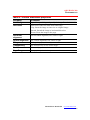
Settings
Flag wells outside
range
Mark as outlier
Show red rectangle indicator inside the grid if the
threshold conditions meet the criteria.
Mark flagged data as outlier
Threshold Options
Manual
Use raw value or concentration value for threshold conditions (Figure 4.43).
Flag the wells
outside of this
range.
Combination
selection is
allowed.
Figure 4.43 Manual threshold tab
LLOD(Lower Limit of Detection)
Flag the lower values than the LLOD calculation value (Figure 4.44). LLOD
is based on the Response Value mean value of the selected wells plus the
standard deviation multiplied by the user selected number.
Select the base
Response Value
wells from pop up
well grid.
Figure 4.44 LLOD tab
®
MasterPlex
ReaderFit www.miraibio.com
72
CHA PT E R 4
DEFINING A PLATE
ULOD(Upper Limit of Detection)
Flag the upper values than the ULOD calculation value (Figure 4.45). ULOD
is based on the MFI mean value of the selected wells plus the standard
deviation multiplied by the user selected number.
Select the base
MFI wells from
pop up well grid.
Figure 4.45 ULOD tab
CV
Use %CV value of the group as a threshold criterion (Figure 4.46). Flag the
values greater than the specified %CV value.
Figure 4.46 %CV tab
®
MasterPlex
ReaderFit www.miraibio.com
73
CHA PT E R 4
DEFINING A PLATE
Extrapolated Values
Flag the values extrapolated by the standard curves (Figure 4.47).
Figure 4.47 Extrapolated values tab
®
MasterPlex
ReaderFit www.miraibio.com
74
CHA PT E R 5
STANDARD CURVES & CONCENTRATION
CHAPTER
5
Standard Curves & Concentrations
- Fit Curve tab
This chapter explains how to generate standard curves and compute
(interpolate or extrapolate) analyte concentrations from the standard curves.
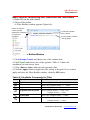
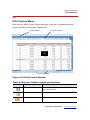
5.1
Go to Fit Curves Tab
Click Fit Curves tab then application window displays the Fit Curves tab
page (Figure 5.1).
Fit Curves tab
Standard Data
Group pane
Standard Curve Data Grid and Chart
Commands and
Display Options
Figure 5.1 Fit Curves page
®
MasterPlex
ReaderFit www.miraibio.com
75
CHA PT E R 5
STANDARD CURVES & CONCENTRATION
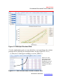
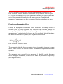
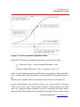
Each well in a standard data set represents an x,y data point. The Response
value is plotted on the y-axis and the concentration is plotted on the x-axis.
MasterPlex® ReaderFit uses nonlinear regression (curve fitting) analysis to fit
a user-specified model equation to the standard data set and generate a
standard curve.
NOTE: The standard curve may not pass through each point in the standard data
set.
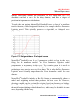
The software computes the R2 value (0 ≤ R2 ≤ 1) for the model equation. R2
measures the goodness of fit of the model equation to the standard data set
(where R2 = 1 is the probability that the model predicts the data perfectly).
The steps to create a standard curve include:
1. Mark the standard wells.
2. Link the standard data set to the unknown well group(s) of interest.
(The analyte concentrations are interpolated from the standard curve that is
linked to the unknown well group.)
4. Enter the standard concentrations.
5. Select a model equation for the standard data set.
6. Calculate the standard curves.
NOTE: A plate can have more than one standard data set. The standard data sets
may have different concentrations or model equations.
®
MasterPlex
ReaderFit www.miraibio.com
76
CHA PT E R 5
STANDARD CURVES & CONCENTRATION
Selecting a Model Equation for the Standard Data Set
1. Select an analyte from the left analyte pane.
2. In the right pane, select one equation from the drop-down list.
Equation symbol is shown under the drop-down list (Figure 5.2).
Figure 5.2 Model Equations drop-down list
Model equations available for regression analysis of a standard data set
3. Select a model equation.
4. To apply the selected model to all analytes, choose the Select for all
analytes option.
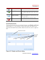
5. To apply weighting during curve fitting, choose the Use Weighting option
and select a weighting method from the drop-down list.
6. To fix the lower asymptote to zero (sets A = 0), select the Fixed lower
asymptote zero option (Figure 5.3). This is an option of the Five Parameter
Logistics and Four Parameter Logistics equations.
NOTE: This feature is reasonable to use if enough background was subtracted and
the data has little user error, but for most data sets the R2 and concentration values
will not be improved with this feature on.
Figure 5.3 Weighting and Fixed asymptote option
Model equations available for regression analysis of a standard data set
NOTE: For more information about model equations and weighting methods, see
Appendix C.
®
MasterPlex
ReaderFit www.miraibio.com
77
CHA PT E R 5
STANDARD CURVES & CONCENTRATION
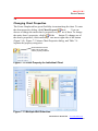
5.2
Generating Standard Curves & Computing
Analyte Concentrations
MasterPlex® ReaderFit carries out a two step calculation sequence when it fits
the standard curves. The software:
• Fits a standard curve for all defined standard data sets
• Interpolates or extrapolates analyte concentrations for the unknown
groups that are linked to the standard data set
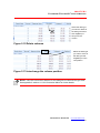
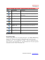
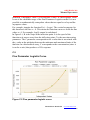
Standard Points Options (Figure 5.4)
Displays each point in the standard data set
Individual points
individually on the standard curve chart.
(default)
Average standards
Displays averaged data points within the same
standard values, with an error bar.
Figure 5.4 Standard Points option
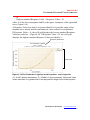
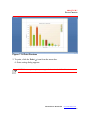
Standard Points Options (Figure 5.5)
Plot X-axis data on the chart by log scale
Set X-axis to log scale
Set Y-axis to log scale
Plot X-axis data on the chart by log scale
Plot unknown wells
Plot unknown wells on the curve
Figure 5.5 Chart Scale option
®
MasterPlex
ReaderFit www.miraibio.com
78
CHA PT E R 5
STANDARD CURVES & CONCENTRATION
Generating Standard Curves
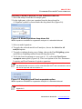
1. To generate the standard curves and compute (interpolate or extrapolate) the
analyte concentrations, click the Calculate button
.
A message box confirms the calculations are completed (Figure 5.6).
Figure 5.6 Message box
Generating Standard Curves by using Best Fit
1. To generate the standard curves and compute the analyte concentrations by
using Best Fit feature, check ‘Use Best Fit feature’ on (Figure 5.7), then
click the Calculate button
.
A message box confirms the calculations are completed (Figure 5.6).
Figure 5.7 Best Fit feature check box
NOTE: If overall R-square value is less than 0.9, a warning message box appears
(Figure 5.8).
Figure 5.8 Warning Message box
®
MasterPlex
ReaderFit www.miraibio.com
79
CHA PT E R 5
STANDARD CURVES & CONCENTRATION
5.3
Reviewing Calculated Standard Data
1. Standard data grid and Standard chart view are updated (Figure 5.7).
Figure 5.9 Standard Data Table and Chart
2. To view multiple standard data, select the analyte from the analyte pane
during [CTRL] key pressing down.
Data table and chart are updated by the multiple standard (Figure 5.8).
®
MasterPlex
ReaderFit www.miraibio.com
80
CHA PT E R 5
STANDARD CURVES & CONCENTRATION
Figure 5.10 Multiple Standard Data
2. In the standard data grid, you can add, delete, sort, interchange the column
position and set filtering for customized data viewing (Figure 5.9, 10, 11).
There are 15 data types available to review (Table 5.1).
Select one of the
data types from the
pop-up menu and
drag&drop it onto the
data grid where you
would like to add the
column.
Figure 5.11 Add column from column chooser box
®
MasterPlex
ReaderFit www.miraibio.com
81
CHA PT E R 5
STANDARD CURVES & CONCENTRATION
Select the data type
you want to delete in
the data grid column
and drag&drop it
away from the
column.
Figure 5.12 Delete columns
Select the data type
you want to move in
the data grid and
drag&drop it to the
new position.
Figure 5.13 Interchange the column position
NOTE: There are some other features for the data gird to customize the gird view.
See appendix A section A.1 Grid Customize Menu for further details.
®
MasterPlex
ReaderFit www.miraibio.com
82
CHA PT E R 5
STANDARD CURVES & CONCENTRATION
Table 5.1 Data Types in the well grid
Data Type
Description
Well
Analyte
Sample Name
Replicate Group
Name
Ignored
Well name
Analyte name
User-specified name for the well.
The group number of the well. Wells that belong to the
same group have the same group number.
If this is checked, this data is not included for the regression
analysis.
The light intensity measured by the plate reader instrument.
Background subtracted value from Response Value.
Response Values
Response ValuesBackground
Response Mean
Response SD
Response %CV
Calculated
Independent
Values
Calculated Mean
Calculated SD
Calculated %CV
Residuals
%Recovery
Background
Shows the Response Value average within the group.
Shows the Response Value standard deviation within the
group.
Shows the Response Value %CV within the group.
The concentration that is calculated (interpolated or
extrapolated) from the user-selected standard curve.
Standard data user inputted.
Shows the concentration average within the group.
Shows the concentration standard deviation within the
group.
Shows the concentration %CV within the group.
Residual = Observed (or calculated) concentration –
Expected concentration
%Recovery = (Calculated/Expected) x 100.
Response Value background value for the plate.
4. Check the fitted curve on the standard curve chart (Figure 5.12).
If the standard curve uses a sigmoidal model (for example, the Four Parameter
Logistics equation, Figure 5.12), the software interpolates the analyte
concentration when:
Highest standard Response Value ≤ Response Value ≤ Lowest standard
data point
The software extrapolates the analyte concentration when:
A < Response Value < Lowest standard Response Value
®
MasterPlex
ReaderFit www.miraibio.com
83
CHA PT E R 5
STANDARD CURVES & CONCENTRATION
or
Highest standard Response Value < Response Value < D
where A is the lower asymptote and D is the upper asymptote of the sigmoidal
curve (Figure 5.12).
A Response Value less than A or greater than D is beyond the range of the
standard curve model and the concentration value cannot be extrapolated.
If Response Value < A, the well grid displays the lowest standard Response
Value preceded by < (Figure 5.12). If Response Value > D, the well grid
displays the highest standard Response Value preceded by >.
Equation parameters
Chart area
Figure 5.14 Five Parameter Logistics model equation, x-axis log scale
A = 38.367 (bottom asymptote), D = 22988.119 (top asymptote). Response Value
values less than A or greater than D are beyond the range of the model equation.
®
MasterPlex
ReaderFit www.miraibio.com
84
CHA PT E R 5
STANDARD CURVES & CONCENTRATION
Specifying Outliers for Standard Data Point
1. Click one of the data points on the chart you want to eliminate from the
calculation (Figure 5.13).
Small data window pops up under the cursor and the corresponding data
is highlighted in the data table (Figure 5.16).
Data pop up window
Figure 5.15 Click one of the data points on the chart
Figure 5.16 Corresponding Data is highlighted
2. Check the corresponding box in the ignored column by clicking on it (Figure
5.15).
Figure 5.17 Check on the box by clicking
®
MasterPlex
ReaderFit www.miraibio.com
85
CHA PT E R 5
STANDARD CURVES & CONCENTRATION
5.4
Best Fit Calculation Option
ReaderFit has an advanced feature called BEST FIT. This feature finds the
best equation model and weighting combination for your standard data
automatically, and does this for all analytes.
1. Go to Input Data tab.
2. Click the BEST FIT
button.
Progress window appears and MasterPlex® begins searching for the best
combination (Figure 5.16).
Figure 5.18 Progress Window for BEST FIT Calculation
3. Once the best fit has been found for all analytes and all calculations have
been done, the Fit Curves tab is displayed. (Figure 5.17).
Figure 5.19 Notification Dialog of BEST FIT calculation
®
MasterPlex
ReaderFit www.miraibio.com
86
CHA PT E R 5
STANDARD CURVES & CONCENTRATION
Best Fit method options
Best Fit search is based on the index value selected in the preference dialog.
There are three searching index available in the preference dialog.
Root Mean Square
Error (RMSE)
Use RMSE index to choose the best curve fit
combination.
R-Square
Use R-square to choose the best combination.
Least deviation of %
Use LD of % Recover to choose the best. This index
is good for the needs of lower concentration
accuracy.
Recovery
®
MasterPlex
ReaderFit www.miraibio.com
87
CHA PT E R 5
STANDARD CURVES & CONCENTRATION
5.5
Statistics Toolbox
The Statistic Toolbox has a EC(effective concentration) or IC(inhibition
concentration) value list (Figure 5.20). MasterPlex® ReaderFit calculates the
EC or IC value whenever the fitting curve is drawn. You can check the default
EC50 or IC50 value from here or you can add any percentage value you want to
check.
Figure 5.20 EC or ICanything list
Adding a percentage
1. Choose EC or IC you want to display by the radio button.
2. Click the text box above Add button, and then input desired value.
3. Click Add button
MasterPlex® QT calculates the EC or IC value based on the inputted
value and add the result in the list.
®
MasterPlex
ReaderFit www.miraibio.com
88
CHA PT E R 5
STANDARD CURVES & CONCENTRATION
5.6
Printing and Exporting the Standard Data
You can print or export the chart and data table of the standard data.
1. Click the Print
button.
Print preview window appears (Figure 5.21).
Figure 5.21 Print Preview window
2. To pint this, click Print
icon from the menu bar.
Print setting dialog appears.
®
MasterPlex
ReaderFit www.miraibio.com
89
CHA PT E R 5
STANDARD CURVES & CONCENTRATION
3. To export this, click Export Document
drop-down icon.
There are 8 file types and 7 image types to export the document (See
appendix A section A.2 Print Preview Menu for further details and task
options).
NOTE: You can also copy or export the Standard Curve chart by right clicking the
mouse button on the chart. It will show ‘Copy’ and ‘Export Image’ in the pop-up
menu. The ‘Copy’ menu enables you to copy the chart image in bitmap format.
®
MasterPlex
ReaderFit www.miraibio.com
90
CHA PT E R 5
STANDARD CURVES & CONCENTRATION
CHAPTER
6
Reviewing Data – View Results tab
View Results tab is to review the data across all analytes. In this tab, you can:
• Add or delete the data column via column selector box
• Sort or filter the column data
• Change the column layout
• Make groups to categorize the data
• Print or export the data
View Results tab
Figure 6.1 View Results Table
®
MasterPlex
ReaderFit www.miraibio.com
91
CHA PT E R 5
STANDARD CURVES & CONCENTRATION
6.1
Add or Delete a column
1. Click Show Columns Selector
Column selector appears(Figure 6.2).
button.
Figure 6.2 Column Selector box
2. To add a data column, select one of the data types and drag & drop it onto
the data grid (Figure 6.3)
Figure 6.3 Add data type to the data grid
3. To delete the column from the data grid, select desired column and drag &
drop it away from the column (Figure 6.4).
®
MasterPlex
ReaderFit www.miraibio.com
92
CHA PT E R 5
STANDARD CURVES & CONCENTRATION
Figure 6.4 Delete data type from the data grid
Table 6.1 Data Types in the Data Table
Data Type
Description
Well
Analyte Name
Sample Name
Replicate Group
Name
Outlier
Response Values
Response Values Background
Response Mean
Response SD
Well name
Analyte name
User-specified name for the well.
The group number of the well. Wells that belong to the
same group have the same group number.
Well data are not included in the calculation.
The light intensity measured by the plate reader instrument.
Background subtracted value from Response Value.
Response %CV
Calculated
Independent
Values
Calculated Mean
Calculated SD
Calculated %CV
Residuals
%Recovery
EC50 / IC50
Dilution Factor
Shows the Response Value average within the group.
Shows the Response Value standard deviation within the
group.
Shows the Response Value %CV within the group.
The concentration that is calculated (interpolated or
extrapolated) from the user-selected standard curve.
Standard data user inputted.
Shows the concentration average within the group.
Shows the concentration standard deviation within the
group.
Shows the concentration %CV within the group.
Residual = Observed (or calculated) concentration –
Expected concentration
%Recovery = (Calculated/Expected) x 100.
Half maximal effective concentration (EC50), half maximal
inhibitory concentration (IC50)
Dilution factor for Background, Unknown and Control.
®
MasterPlex
ReaderFit www.miraibio.com
93
CHA PT E R 5
STANDARD CURVES & CONCENTRATION
6.2
Sort or Filter the Column Data
To sort by specific column, click the column title. Ascending and descending
are changed alternatively (Figure 6.5).
Ascending sort
Descending sort
Figure 6.5 Sort Column Data
To clear the sort, right click on the column you want to clear the sort, select
‘Clear Sorting’ from the menu (Figure 6.6).
Figure 6.6 Clear Sorting
®
MasterPlex
ReaderFit www.miraibio.com
94
CHA PT E R 5
STANDARD CURVES & CONCENTRATION
To filter by specific data in the column, click upper right side of the column
you want to use it as filter base (Figure 6.7).
Figure 6.7 Filter by the data in the column
NOTE: There is a way to construct more complex filter conditions using Filter
Builder. See appendix A section A.1 ‘Create Complex Filter Criteria’ paragraph.
®
MasterPlex
ReaderFit www.miraibio.com
95
CHA PT E R 7
DATA CHARTS
6.3
Exporting a Data
You can export your data table data from Export to File button
.
1. Click Export to File drop-down button.
2. Select the file format you want to export
There are five file formats available: Excel, CSV, PDF, HTML and Text
(Figure 6.8).
Figure 6.8 Export to File menu
3. File save dialog appears. Set file path and input file name, then click OK
(Figure 6.9).
Figure 6.9 File save dialog
®
MasterPlex
ReaderFit www.miraibio.com
96
CHA PT E R 7
DATA CHARTS
4. After saving the file, an Open file prompt appears (Figure 6.10). If you want
to open the saved file immediately using the program the files extension is
associated with, click Yes.
The saved file is opened on the program. (Figure 6.11).
Figure 6.10 Confirmation dialog
Figure 6.11 Opening in Excel
®
MasterPlex
ReaderFit www.miraibio.com
97
CHA PT E R 7
DATA CHARTS
6.4
Printing a Data
You can preview your data with the Print Preview button
1. Click the Print Preview button.
Print preview window appears (Figure 6.12).
.
Figure 6.12 Print Preview
2. To print, click the Print
icon from the menu bar.
Print setting dialog appears.
NOTE: For more printing options, see appendix A section A.2 ‘Print Preview’ menu.
®
MasterPlex
ReaderFit www.miraibio.com
98
CHA PT E R 7
DATA CHARTS
CHAPTER
7
Data Charts – Create Graphs tab
MasterPlex® ReaderFit can display Response Value, concentration or
standard data in many graph formats in the create graphs tab.
Create Graphs tab
Figure 7.1 Create Graphs tab
7.1
Viewing a Data Chart
1. Click the Well Selector
button.
Α mini sized well plate is displayed under the button (Figure 7.2).
®
MasterPlex
ReaderFit www.miraibio.com
99
CHA PT E R 7
DATA CHARTS
Figure 7.2 Well Selector
2. Select the wells you want to display on the chart. You can select multiple
wells by pressing [CTRL] key (Figure 7.3).
Figure 7.3 Multiple Well Selection
Figure 7.4 Bar Chart for Selected Wells
®
MasterPlex
ReaderFit www.miraibio.com
100
CHA PT E R 7
DATA CHARTS
3. To display another data type for the selected wells, click the Data Type
drop-down list and select one of the data type.
Table 7.1 Data Types
Data Type
Displays...
Response Value
Concentration
Response Value
Calculated concentration
4. To change the data type, click the Chart Type drop-down list and select one
of two chart types.
Table 7.2 Chart Types
Chart Type
Displays...
Well Group
Wells by Analyte
Analyte data for each user selected well.
Analyte data for each user selected well by
analyte.
Wells per Analyte
Analyte data for each user selected well per
analyte.
Group by Analyte
Plot the selected data type which has sample
name, across the analytes. (Figure 7.5)
Group by Sample Name Plot the selected data type which has sample
name, across the sample name. (Figure 7.6)
®
MasterPlex
ReaderFit www.miraibio.com
101
CHA PT E R 7
Response Values
DATA CHARTS
Response Values
Figure 7.5 Group by Analyte chart
Figure 7.6 Group by Sample name chart
®
MasterPlex
ReaderFit www.miraibio.com
102
CHA PT E R 7
DATA CHARTS
Replicate View
Plotting group values is available by clicking the Replicate View button
.
Replicate View is available only on Bar style charts. If you are on another
type of chart when you click the Replicate View button, it automatically
re-selects the Bar chart and displays the data with error bars. Figure 7.7 shows
an example of the replicate view chart.
Average
+Stdev
Average
value
Response Values
Average
-Stdev
Figure 7.7 Replicate View chart
®
MasterPlex
ReaderFit www.miraibio.com
103
CHA PT E R 7
DATA CHARTS
7.2
Chart Format
MasterPlex® ReaderFit provides various chart formats (Table 7.3). To change a
chart format for the selected well data, click the Chart Gallery button
,
and make a selection from the drop-down list of Chart Gallery.
Table 7.3 Available chart format
Icon Chart Name
Features
Bar
Bar style x-y chart
Bar 3D
3D bar style x-y chart
Manhattan Bar
3D bar style x-y-z chart
Point
Point style x-y chart
Line
Line interpolated style x-y chart
Step Line
Step line interpolated style x-y chart
Spline
Spline interpolated style x-y chart
Line 3D
3D line interpolated style x-y chart
Step Line 3D
3D step line interpolated style x-y chart
Spline 3D
3D spline interpolated style x-y chart
Area
Are painted style x-y chart
Spline Area
Spline area painted style x-y chart
Area 3D
3D area painted style x-y chart
Spline Area 3D
3D spline area style x-y chart
Pie
Pie style circular chart
Pie 3D
3D pie style circular chart
Doughnut
Doughnut style circular chart
Doughnut 3D
3D doughnut style circular chart
Radar Line
Line interpolated style radar chart
Radar Point
Point plotted style radar chart
®
MasterPlex
ReaderFit www.miraibio.com
104
CHA PT E R 7
DATA CHARTS
7.3
Analyte Selector
In the Well Group chart, Analyte Selector allows you to change the analytes
position in the chart and allows you to display on/off setting for each analyte.
To move the analyte position,
1. Click Analyte Selector drop-down list (Figure 7.8).
2. Select the analyte you want to move.
3. To move the analyte to the left, click Up button. To move the analyte to
right, click Down button.
The analyte moves one position to the left (or right) from its current
position (Figure 7.9).
In the Single Analyte chart, the Analyte Selector allows you to select the
analyte you want to display in the chart (Figure 7.10).
All Analytes in the
plate. To turn the
display of the
analyte on or off,
check the box next
to it.
Figure 7.8 Analyte Selector drop-down list
®
MasterPlex
ReaderFit www.miraibio.com
105
CHA PT E R 7
DATA CHARTS
Response Values
Response Values
Select the analyte
and click the
‘Down’ button.
Figure 7.9 Change the analyte position
All Analytes in the
plate. To select the
analyte, click the
radio button next to
the analyte name.
Figure 7.10 Analyte Selector drop-down list
®
MasterPlex
ReaderFit www.miraibio.com
106
CHA PT E R 7
DATA CHARTS
7.4
Changing the Color Palette
There are 30 color palettes available from Color Palette button
. Figure
7.11 shows the palette names and their corresponding color patterns.
Figure 7.11 Color Palettes
®
MasterPlex
ReaderFit www.miraibio.com
107
CHA PT E R 7
DATA CHARTS
7.5
Changing Chart Properties
The Create Graphs tab has great flexibility in customizing the chart. To enter
the chart properties dialog, click Chart Properties button
. You can
choose to change the entire chart’s properties or just one of them. To change
the entire chart’s properties, click body of the
button. To change one of
the chart’s properties, click small drop-down arrow right side of the button
(Figure 7.12) . Figure 7.13 shows Chart Properties dialog, and Table 7.4
explains the property categories.
Click small down arrow
mark to show the each
chart’s property selection.
Response Values
Figure 7.12 Chart Property for Individual Chart
Figure 7.13 Multiple Well Selection
®
MasterPlex
ReaderFit www.miraibio.com
108
CHA PT E R 7
DATA CHARTS
Table 7.4 Chart Properties
Properties Icon Features
Legends
Customize the legend’s properties.
Diagram
Axes
Chart Titles
Point Labels
Series Views
Appearance
Customize the diagram’s properties.
Customize X and Y axes of the diagram. Note that
you may select an axis to be modified on the chart
preview.
Add chart titles to be displayed within a chart.
Customize point label properties of the selected
series. Note that you may select a series to be
modified on the chart preview.
Customize series view properties of the selected
series. Note that you may select a series to be
modified no the chart preview.
Choose a palette to color series or their data points.
Also choose the style, which specifies the chart’s
appearance depending on the current palette.
7.6
Printing a Chart
You can print your data with the Print button
.
1. Click the Print Preview button.
Print preview window appears (Figure 7.14).
®
MasterPlex
ReaderFit www.miraibio.com
109
CHA PT E R 7
DATA CHARTS
Figure 7.14 Print Preview
2. To print, click the Print icon from the menu bar.
Print setting dialog appears.
NOTE: For more print options, see appendix A section A.2 ‘Print Preview’ menu.
®
MasterPlex
ReaderFit www.miraibio.com
110
CHA PT E R 7
DATA CHARTS
7.7
Copying or Saving Chart Image
The software can export the chart image to other applications. The data may
be copied to the system clipboard or saved in different file formats.
1. Right click on the chart you want to copy or save.
2. To copy the chart image in bitmap format, click ‘Copy’.
The image is sent to the clipboard and you can paste the image data on
other applications.
3. To save the chart image in other formats, click ‘Export Image’.
The File Save dialog is opened (Figure 7.15).
4. Input the file name and select one of the file formats from the ‘Save as type’
drop-down list. There are five formats available: bitmap, png, html, pdf and
Excel.
Figure 7.15 Chart Image Export dialog
®
MasterPlex
ReaderFit www.miraibio.com
111
CHA PT E R 8
EXPORT DATA
CHAPTER
8
Export Data – Customized Report Manager tab
This chapter explains how to export MasterPlex® ReaderFit data transformed
by the user. Custom report is a powerful and flexible tool for presenting and
exporting your data. Compared to regular report, Custom report has greater
flexibility on what and how to present data. While ReaderFit stores its
analysis results in an XML format document, it is possible for users to present
their data in whatever format they want. The only thing users need to do is to
define their presenting formats in XSL files (Extensive Stylesheet Language).
Figure 8.1 Customized Report Manager tab
®
MasterPlex
ReaderFit www.miraibio.com
112
CHA PT E R 8
EXPORT DATA
8.1
Importing a User Defined Stylesheet
1. Click Import button
.
The file open dialog appears (Figure 8.2).
Figure 8.2 Open File Dialog
2. Select the file you want to import to the Customized Report Manager.
Style sheet’s name is displayed in the Style Sheet list, and XSL
Information window shows style sheet’s information (Figure 8.3).
®
MasterPlex
ReaderFit www.miraibio.com
113
CHA PT E R 8
EXPORT DATA
Figure 8.3 Style Sheet List and Information
8.2
Exporting a User Defined Stylesheet
1. Click Export button
.
The file save dialog appears (Figure 8.4).
®
MasterPlex
ReaderFit www.miraibio.com
114
CHA PT E R 8
EXPORT DATA
Figure 8.4 Save File Dialog
2. Set the destination and input file name, then click the Save button.
Style sheet’s name is displayed in the Style Sheet window, and XSL
Information window shows style sheet’s information (Figure 8.3).
8.3
Delete Style Sheet File from Style Sheet List
1. Select the style sheet you want to delete from the style sheet list.
2. Click the Delete button
.
The confirmation dialog appears (Figure 8.5).
3. Click OK to delete.
®
MasterPlex
ReaderFit www.miraibio.com
115
CHA PT E R 8
EXPORT DATA
Figure 8.5 Confirmation Dialog
8.4
Including standard curve images
1. Check Include standard curve images.
The transformed data includes standard curve image data as base64
encoding.
8.5
Transform Original Data into Your Customized Data
1. Select the style sheet you want to apply from the style sheet list.
2. Click the Apply button
.
The transformed data is shown in the preview window (Figure 8.6).
®
MasterPlex
ReaderFit www.miraibio.com
116
CHA PT E R 8
EXPORT DATA
Figure 8.6 Transformed Data (HTML format)
3. Save to file or print from the menu button.
®
MasterPlex
ReaderFit www.miraibio.com
117
APPENDIXA
PREFERENCES
APPENDIX
A
This appendix explains more details about Data Grid (for Fit Curves tab and
View Results tab) and Print Preview.
A.1
Grid Customize Menu
Grid customize menu allows you to customize your grid data viewing more
flexibly and efficiently. Grid Customize Menu is invoked by right clicking on
the both grid column, standard curve data grid and data table grid (Figure A.1).
Figure A.1 Grid Menu in the Fit Curves tab and View Results tab
Table A.1 Main toolbar buttons and functions
Icon
Command
Function
Sort Ascending
Sort right clicked column by ascending.
Sort Descending
Sort right clicked column by descending.
Clear Sorting
Clear sorting of right clicked column (if the
®
MasterPlex
ReaderFit www.miraibio.com
118
APPENDIXA
PREFERENCES
columns is sorted).
Group By This Column
Make a group by right clicked column. The
group is located under the last position of
current group hierarchy.
Hide Group By Box
Display/Hide Group Box (Figure A.2) on the
upper side of the columns. It enables you to
make group(s) by drag and drop operation.
Remove This Column
Remove right clicked column.
Column Chooser
Show Column Chooser box.
Best Fit
Adjust the width of right clicked column.
Clear Filter
Clear filter condition of right clicked column
(if column is filtered).
Filter Editor
Open Filter Builder window (Figure A.6).
Best Fit (all columns)
Adjust the width of all columns.
Group Box
The Group Box appears on the upper side of the column (Figure A.2) by
choosing the Group By Box menu from the right click menu on the grid
column. You can drag one of the column you want to group to this box (Figure
A.3). Also you can multi-group by repeating same way (Figure A.4).
Figure A.2 Group Box
®
MasterPlex
ReaderFit www.miraibio.com
119
APPENDIXA
PREFERENCES
Figure A.3 Group by Drag & Drop
Replicate Group Name
Figure A.4 Multi-Group by Drag & Drop
®
MasterPlex
ReaderFit www.miraibio.com
120
APPENDIXA
PREFERENCES
Group Box Menu
Group Box has context menu. Table A.2 shows the menus.
Table A.2 Main toolbar buttons and functions
Icon
Command
Function
Full Expand
Expand all group trees.
Full Collapse
Collapse all group trees.
Clear Grouping
Clear group and return the group columns to
the grid column..
Working with Column Filter
There are two ways to set a filter. The first way is by using the filter
drop-down menu from the column (Figure A.5). You can filter the column by
selecting the specific data in the column. The second way is by using the
Filter Builder window (Figure A.6).
Figure A.5 Direct Filtering from the column
®
MasterPlex
ReaderFit www.miraibio.com
121
APPENDIXA
PREFERENCES
Create Complex Filter Criteria
To construct filter criteria involving multiple columns and various comparison
operators, use the filter drop-down list and click Custom. This invokes the
Custom AutoFilter dialog (Figure A.6) which allows you to compare a column
with one or two values. To construct using more various operators and
multiple conditions, use the filter builder. See ‘Basic step for constructing
Filter Criteria by using Filter Builder’ paragraph in this section.
Figure A.6 Custom AutoFilter dialog
Filter Builder Window
By using the filter builder, you can filter the data more specifically. To open
the filter builder window, choose Filter Editor from the right click menu on
the column or click Edit Filter button on the bottom of the data grid (Figure
A.7).
Figure A.7 Opening the Filter Builder
®
MasterPlex
ReaderFit www.miraibio.com
122
APPENDIXA
PREFERENCES
Basic steps for constructing filter criteria with the Filter Builder
1. Right click on the grid column.
2. Choose Filter Editor.
Filter Builder window appears (Figure A.8).
Click to change the
current operator,
add/remove conditions
and groups of
conditions.
To add filter condition,
click [+] button.
To remove filter condition,
click [x] button.
Figure A.8 Filter Builder Window
3. Click [Sample Name] and choose one of the column item.
4. Click Equals and choose one of the operator. Table A.3 shows the
conditions you can choose from.
5. Click <Enter a value> and enter the operand value.
6. Click the Apply button to apply the filter setting to the grid. If you want to
apply and close the Filter Builder window, click the OK button.
Table A.3 Available Commands for Filter
Icon Operator
Function
Equals
Shows only [Sample Name] = <value>.
Does not equal
Shows only [Sample Name] ≠ <value>
Is greater than
Shows only [Sample Name] > <value>.
Is greater than or equal
Shows [Sample Name] = <value> and
[Sample Name] > <value>
Is less than
Shows only [Sample Name] < <value>
Is less than or equal
Shows [Sample Name] = <value> and
[Sample Name] < <value>
®
MasterPlex
ReaderFit www.miraibio.com
123
APPENDIXA
PREFERENCES
Is between
Shows only the value which has between first
<value> and second <value>
Is not between
Shows only the outside value which has between
first <value> and second <value>
Contains
Shows only the value contains <value>
Does not contain
Shows only the value does not contains <value>
Begins with
Shows only the value starts with <value>
Ends with
Shows only the value ends with <value>
Is like
Shows only [Sample Name] > <value>
Is not like
Shows only [Sample Name] > <value>
Is blank
Shows only value are blank.
Is not blank
Shows only value are not blank.
Is any of
Shows only value which has <value>s.
Is none of
Shows only value does not have <value>s.
Shows only,
Analyte name is ‘IL-10’ and Response Value is between 100
and 500,
or
Analyte name is ‘IL-6’ and Response Value is less than
Figure A.9 Example of the complex filter criteria
®
MasterPlex
ReaderFit www.miraibio.com
124
APPENDIXA
PREFERENCES
A.2
Print Preview Menu
Print preview allows you to zoom, navigate, print out, set printing options,
export and other useful tasks (Figure A.10).
Preview Menu
Preview Toolbar
Preview
Area
Preview Status Bar
Figure A.10 Print Preview Window
Table A.4 Preview Toolbar buttons and functions
Icon
Command
Function
Search
Search specific word or value from the
preview document.
Customize
Customize the printing items.
Open
Open preview document files(*.prnx).
®
MasterPlex
ReaderFit www.miraibio.com
125
APPENDIXA
PREFERENCES
Save
Save preview document by *.prnx format.
Print…
Open print dialog.
Print
Print the preview document.
Print Setup…
Open print setup dialog.
Header and Footer
Set up header and footer options (Figure A.10).
Scale
Set page scale.
Hand Tool
User hand icon
Magnifier
User magnifier
Zoom Out
Zoom out the preview document.
Zoom
Set zoom size from the drop-down list.
Zoom In
Zoom in the preview document.
First Page
Show first page.
Previous Page
Show previous page.
Next Page
Show next page
Last Page
Show last page.
Multiple Pages
Select multi pages to preview.
Color…
Open color picker and set the document
background color.
®
MasterPlex
ReaderFit www.miraibio.com
126
APPENDIXA
PREFERENCES
Water Mark…
Open water mark setting dialog (Figure A.10).
Export Document…
Export the document by selected format.
PDF, HTML, MHT, RTF, Excel, CSV, Text,
Image
Send via E-Mail…
Export the document by selected format, and
send it via e-mail.
PDF, MHT, RTF, Excel, CSV, Text, Image
Exit
Close preview window.
Insert Header/Footer
To insert header/footer into your printing document, open Header and Footer
dialog (Figure A.11). Select header or footer radio button, then input text or
items from the header/footer toolbar (Table A.5) in the left, center or right text
box.
Header/Footer toolbar
Left, center
and right
text box
Figure A.11 Header and Footer dialog
®
MasterPlex
ReaderFit www.miraibio.com
127
APPENDIXA
PREFERENCES
Table A.5 Header and Footer Toolbar buttons and functions
Icon
Command
Function
Page Number
Insert page number.
Page # of Pages #
Insert ‘(current page) of (total pages)’ type
page number.
Date Printed
Insert date printed.
Time Printed
Insert time printed.
User Name
Insert user name who login the windows.
Image
Insert the image.
Align to Top
Align all headers/footers to the top level.
Align to Center
Align all headers/footers to the center level.
Align to Bottom
Align all headers/footers to the bottom level.
Font
Open font dialog for the header and footer font.
Insert Water Mark
To insert water marks into your printing document, open Water Mark dialog
(Figure A.12). There are two types of watermarks you can insert in your
document, one is ‘Text’ and another is ‘Picture’. They are separated into two
tabs. To insert a text watermark, use ‘Text Watermark’ tab. To insert a picture
watermark, use the ‘Picture Watermark’ tab.
®
MasterPlex
ReaderFit www.miraibio.com
128
APPENDIXA
PREFERENCES
Figure A.12 Watermark dialog
Table A.6 Text Watermark properties
Property
Function
Text
Input text word in the text box or select predefined words from
the drop-down list
Predefined words: ASAP, CONFIDENTIAL, COPY, DO NOT
COPY, DRAFT, EVALUATION, ORIGINAL, PERSONAL,
SAMPLE, TOP SECRET, URGENT
Direction
Select text direction from one of the followings:
Horizontal, Vertical, BackwardDiagonal, ForwardDiagonal
Color
Open color picker and choose text font color.
Font
Open font dialog and choose text font.
Size
Specify text font size.
Transparency
Set transparency for the insert text.
Position
Select text position, In front or Behind.
Page Range
Set page range for the text water mark.
®
MasterPlex
ReaderFit www.miraibio.com
129
APPENDIXA
PREFERENCES
Table A.7 Picture Watermark properties
Property
Function
Load image…
Open file open dialog and specify the image file to be inserted.
Size mode
Select one of the size mode from followings.
Clip: Insert the image as same size as original image.
Stretch: Stretch the image to horizontal direction.
Zoom: Zoom the image to the page.
Horizontal
Set horizontal alignment, left, center or right.
alignment
Vertical alignment
Set vertical alignment, left, center or right.
Tiling
Fill up the page by the image.
Transparency
Set transparency for the insert image.
Position
Select image position, In front or Behind.
Page Range
Set page range for the image water mark.
®
MasterPlex
ReaderFit www.miraibio.com
130
APPENDIXA
PREFERENCES
Figure A.13 Example of the text and image watermark
®
MasterPlex
ReaderFit www.miraibio.com
131
APPENDIXB
MASTERPLEX® ReaderFit TOOLBARS
APPENDIX
B
The toolbars that are available depend on the types of windows that are open
in the main display area.
B.1
Main File Menu and Toolbar
Table B.1 Main File menu and toolbar
Menu Bar
Main
Function
Command
Toolbar
Button
File New
Open blank plate for ReaderFit application.
File Open
Displays the Open dialog box so that a results file
(.csv, .txt or .xls), MasterPlex® ReaderFit file
(.mxqs) may be opened.
File Close
Close currently opened plate data file.
File Save
Save currently opened plate data.
File Save as
-
Save currently opened plate data as different file
name.
File Recent Files
-
List up the files recently opened.
File Exit
-
Close MasterPlex® application.
Analyte Filter
Valid analyte filter feature.
Virtual Plate
Generate virtual plate. It opens plate dimension
input dialog.
Windows Show
Tab style
Windows Cascade
Windows Tile
-
Set tab style window display
Arrange the window by cascade style.
Arrange the window by horizontal style.
®
MasterPlex
ReaderFit www.miraibio.com
132
APPENDIXB
MASTERPLEX® ReaderFit TOOLBARS
Horizontal
Windows Tile
-
Arrange the window by vertical style.
-
Open user management dialog.
Vertical
Tools User
Management
Tools Log Viewer
(For 21 CFR Part 11 module only)
-
Open log viewer.
(For 21 CFR Part 11 module only)
Tools Verify files
-
Open verification checker dialog.
(For 21 CFR Part 11 module only)
License -
Open application license information dialog.
License Plugins
-
Open plugin license information dialog.
Help Manuals
-
Open manuals folder.
Help Tutorial
-
Open video tutorial.
Help Online
-
Open support URL by the default browser.
-
Display splash screen with application version
Applications
Support
Help About
information.
Look and Feel
-
Change application skins.
®
MasterPlex
ReaderFit www.miraibio.com
133
APPENDIXB
MASTERPLEX® ReaderFit TOOLBARS
B.2
Input Data Tab Toolbar
The Input Data tab toolbar is available on the top of the well grid in the plate
tab.
Figure B.2 Plate toolbar
Table B.2 Plate toolbar buttons and functions
Menu Bar
Toolbar Function
Command
Icon
Mark selected wells as Background.
Background
Standard
Mark selected wells as Standard.
Unknown
Mark selected wells as Unknown.
Control
Mark selected wells as Control.
Unmark
Unmark selected wells.
Subtract
Background
Best Fit
Toggle subtract background function.
Auto Fill
Open Auto Fill dialog.
Link Standard
Make link(s) between standard data and others.
Quality Control
Manager
Open Quality Control Manager.
Start best fit mode.
®
MasterPlex
ReaderFit www.miraibio.com
134
APPENDIXB
MASTERPLEX® ReaderFit TOOLBARS
Template
Manager
Plate
Preferences
Open template manager.
Open plate preference dialog.
B.3
View Results Tab Toolbar
The View Results toolbar is available on the top of the data grid in the View
Results tab.
Figure B.4 Calculation toolbar
Table B.4 Calculation toolbar buttons and functions
Menu Bar
Toolbar Function
Command
Button
Show/Hide Columns
Show or hide columns selector.
Selector
Export to File
Export data table by selected format.
Format: Excel, CSV, PDF, HTML, Text
Print Preview
Open print preview window
Table Template
Open table template manager.
Merge Cells By
Group
Toggle the cell merge mode.
®
MasterPlex
ReaderFit www.miraibio.com
135
APPENDIXB
MASTERPLEX® ReaderFit TOOLBARS
B.4
Create Graphs Tab Toolbar
The chart toolbar is available on the top of the chart view area in the Create
Graphs tab.
Figure B.5 Chart toolbar
Table B.5 Chart toolbar buttons and functions
Menu Bar
Toolbar Function
Command
Button
Toggle replicate view mode.
Replicate View
Analyte Selector
Shows drop-down list for all analytes.
Well Selector
Shows mini-sized plate view.
Chart Gallery
Shows drop-down list of available chart format.
Color Palette
Shows drop-down list of available palette.
Chart Properties
Open chart properties dialog.
Chart Template
Open chart template manager.
Print Preview
Open print preview.
®
MasterPlex
ReaderFit www.miraibio.com
136
APPENDIXB
MASTERPLEX® ReaderFit TOOLBARS
B.5
Customized Report Manager Tab Toolbar
The Customized Report Manager toolbar is available on the top of the preview
area in the Customized Report Manager tab.
Figure B.5 Chart toolbar
Table B.6 Chart toolbar buttons and functions
Menu Bar
Toolbar Function
Command
Button
Print current displayed document.
Print
®
MasterPlex
ReaderFit www.miraibio.com
137
APPENDIXC
MODEL EQUATIONS
APPENDIX
C
This appendix provides background on the Four and Five Parameter Logistic
curves. It also explains how weighting methods can improve the fit of
nonlinear models to data with non-constant variability (heteroscedasticity).
C.1
Four Parameter Logistic Curve
Figure C.1 Four parameter logistics curve
In Figure C.1, the asymptotes D and A are the upper and lower limits of the
model. An asymptote is a value that the function never reaches.
Therefore, the value of a function at or beyond an asymptote cannot be
®
MasterPlex
ReaderFit www.miraibio.com
138
APPENDIXC
MODEL EQUATIONS
predicted. If Response Value ≤ A or Response Value ≤ D, the Response Value
is out of the calculable range of the Four Parameter Logistics model. It is not
possible to mathematically extrapolate values that are equal to or beyond the
asymptote values.
For example, imagine the function F(x) = Log(x). The vertical asymptote for
this function is the line x = 0. This means the function can never reach the line
where x= 0. For example, log(0) cannot be calculated.
In Figure C.1, B is the slope at the inflection point. It is the speed of the
function as it moves away from the inflection point. C is the most interesting
parameter. The C parameter corresponds to the x value that is associated with
the y value at the midpoint between the minimum and maximum limits of the
function. In a biochemical assay, C corresponds to the concentration (since it
is on the x-axis) that produces a 50% response.
C.2
Five Parameter Logistic Curve
Figure C.2 Five parameter logistic curve
®
MasterPlex
ReaderFit www.miraibio.com
139
APPENDIXC
MODEL EQUATIONS
A Five Parameter Logistic curve introduces an additional parameter to the
Four Parameter Logistic model to compensate for asymmetric data. In Figure
C.2, we can see that the curve is not symmetrical because the lower part of the
curve behaves quite differently from the upper portion. The additional
parameter E compensates for this asymmetric behavior and adjusts the curve.
Fixed Lower Asymptote Zero
Usually an asymptote is estimated where a function is tending toward a
constant value. A fixed asymptote is a restriction that tells the function to
never go beyond that value. For example, setting A = 0, as in the ‘Fixed lower
asymptote zero’ option in the Fit Curves tab. It is used with logistic functions,
like the Four Parameter Logistics (4PL) equation shown below.
Four Parameter Logistics Model
The assumption that the lower asymptote is zero is probably incorrect in some
cases, but it allows the user to reduce the number of parameters in the
equation.
The asymptote sets a bound for the parameter. In the 4PL model, there are
lower and upper asymptotes, defined as the A and D parameters respectively
(See diagram below).
®
MasterPlex
ReaderFit www.miraibio.com
140
APPENDIXC
MODEL EQUATIONS
Figure C.1 Four parameter logistics curve
MasterPlex® ReaderFit extrapolates the analyte concentration when:
A < Response Value < Lowest standard Response Value
or
Highest standard Response Value < Response Value < D
where A is the bottom asymptote and D is the top asymptote of the sigmoidal
curve. An Response Value less than A or greater than D is beyond the range of
the
standard curve model and the concentration value cannot be extrapolated.
In the 2-dimensional representation of the curve shown above, Response
Value is the Y-axis value. Theoretically, Response Value cannot be less than
zero. So, setting the lower asymptote to zero is reasonable. But there can be
measured data that actually has some negative Response Values, which can be
®
MasterPlex
ReaderFit www.miraibio.com
141
APPENDIXC
MODEL EQUATIONS
caused by user error.
MasterPlex® ReaderFit provides a function to subtract the background noise
from the Response Values to obtain more accurate responses. If the user
subtracts a reasonable amount of background, it could be assumed that the
lowest detectable Response Value is zero. Note that log(0) is undefined. So, in
some cases, fixing the lower asymptote to zero is theoretically correct.
However, in reality, most datasets contain some slight amount of error, so
fixing the lower asymptote to zero can actually make it more difficult to
achieve a good curve fit. For this reason, a slightly better R2 value is usually
reported when the curve fitting is done with this feature turned off
(unchecked), which is the default, but the difference in the R2 value would be
very small – usually less than 1/100,00th or 0.00001. Any change in the graph
would be unnoticeable. The difference in the interpolated concentrations
would also be very small – usually less than 2% if any.
Asymptotes can be used to gauge the similarity of functions. For example, if
two curves calculated with the Four Parameter Logistics equation end up
having very close to the same A and D parameters, their interpolated
concentrations would be in the same range.
The lower and upper asymptotes (A and D) of the 4PL and 5PL models
usually calculated automatically during the curve fitting process and are
derived from the characteristics of the data. The “Fixed lower asymptote zero”
feature makes it possible to fix the lower asymptote to a hardcoded value of
zero, which is useful in some experiments. This feature is reasonable to use if
enough background was subtracted and the data has little user error. But for
most data sets, the R2 and concentration values will not be improved with this
feature on.
Log-Log Model
The Log-Log model transforms the data to log scale for the x and y values. It
applies linear regression to fit a straight line through these points. This model
is appropriate for data that are intrinsically linear.
®
MasterPlex
ReaderFit www.miraibio.com
142
APPENDIXC
MODEL EQUATIONS
C.3
Heteroscedasticity
Fitting nonlinear models to observed data is often complicated by
non-constant or heterogeneous variability. Heterogeneous variability or
heteroscedasticity occurs in most types of observed data. This is especially
true for biochemical assays where concentration or dose is the predictor.
Therefore, we can expect that measurement error varies with respect to the
mean. In the plate reader system, Response Values are based on vary with the
concentration. In this case, we expect the error in detecting Response Value to
increase as concentration increases. This is best seen in Figure C.3, a residual
plot from a plate reader cytokines assay.
A residual plot is a graphical representation of how far away an observed
concentration is from its expected value. It plots residuals against observed
concentrations. In Figure C.3, we can see that the deviation of the observed
concentration from the expected value increases as concentration increases.
This means the variability is not constant.
Residual plots help you detect non-constant variability as well as outliers. If a
residual plot exhibits data points in a wedge or funnel-shaped pattern, then we
can expect the underlying data to have non-constant variability.
Non-constant variability complicates curve fitting because the regression
process assumes the errors are constant across all data points. When the data
violate this assumption, the resulting curve fit is less than optimal. This is
illustrated in Figure C.4.
®
MasterPlex
ReaderFit www.miraibio.com
143
APPENDIXC
MODEL EQUATIONS
Figure C.4 Data with non-constant variability
The residual increases as concentration increases.
When we fit a model to the data, the curve is applied to all of the data points
as closely as possible so that the distances between the predicted and expected
concentrations are minimized. In Figure C.4 we can think of the lines that
represent the residuals as ropes and each data point as a wrench. Curve fitting
can be imagined as pulling the curve line so that it is as close to each point as
possible without snapping the actual curve.
The best curve fit is reached when the curve is pulled as close as possible to
each data point without breaking the actual curve model.
The nonlinear least square algorithm accomplishes this task. The nonlinear (or
linear) least square algorithm assumes that all points have the same variability,
so all points influence the curve fit equally.
However, data that exhibit non-constant variability violate this assumption. As
a result, data points with greater variability assert more ‘pull’ on the curve.
Data points at higher concentrations have more variability then those at lower
concentrations, and have greater influence on the curve fit than the points at a
lower concentration. As a result, accuracy or sensitivity at the lower
®
MasterPlex
ReaderFit www.miraibio.com
144
APPENDIXC
MODEL EQUATIONS
concentrations decreases.
Levenberg-Marquardt algorithm (LMA)
The Levenberg–Marquardt algorithm (LMA) used by MasterPlex® ReaderFit
minimizes a function over a space of parameters of the function. It is
commonly used in least-square-fitting and nonlinear regression (curve fitting).
LMA interpolates between the Gauss-Newton algorithm (GNA) and gradient
descent. LMA is more robust than GNA, but can be slower for very large
datasets. Robustness is a measure of how well the algorithm can do the curve
fitting with fewer data.
Given two points on a data grid, LMA iteratively takes steps from point 1
towards point 2, adjusting its slope each time. This is harder to visualize in a
multidimensional space, but LMA adjusts in all directions simultaneously as it
fits a multivariate function.
LMA adjusts the parameters of the equation (i.e. the Five Parameter Logistics
or Four Parameter Logistics equations) at each iteration of the algorithm until
there is no improvement in the curve fit, or until it reaches a maximum
threshold (100 iterations in this case). To accomplish the curve fitting, it
combines two common statistical math techniques: Gradient Descent and
Gauss-Newton (GNA).
Gradient Descent: Take steps proportional to the negative of the gradient of
the function at the current point. Each step reduces the sum of squares.
Gauss-Newton (GNA): Determine the amount of change in sum of squares
when each parameter changes. This determines the slope at that point.
Gradient descent usually works well in early iterations, while Gauss-Newton
usually works well in later iterations. LMA automatically switches between
these two methods. The result is a curve fit with a high degree of precision
over a wide variety of datasets. No algorithm can do curve fitting for all
®
MasterPlex
ReaderFit www.miraibio.com
145
APPENDIXC
MODEL EQUATIONS
datasets since some datasets are too sparse or have faulty data. But a good
algorithm can find a curve fit for many datasets, and have a degree of
precision in its parameter calculations.
To track the data points, MasterPlex® ReaderFit uses a class of a nonlinear
transfer function, called a sigmoid function, for example the Five Parameter
Logistics model. This typically produces a sigmoidal, or S-shaped curve
(Figure C.5).
Figure C.5 A sigmoidal or S-shaped curve
MasterPlex® ReaderFit uses 4 or 5 parameters models to help in the curve
fitting for the nonlinear model. The Five Parameter Logistics model
compensates for asymmetry in the curve. To a certain extent, it is useful to
have more parameters to tweak during the curve fitting process, thus
producing a more precise curve to fit the data. This is why the Five Parameter
Logistics model usually outperforms the Four Parameter model for most
datasets.
MasterPlex® ReaderFit includes a Best Fit feature to automatically choose a
model and weighting method that produces the best curve fit. However,
choosing a model can be a scientific decision, based on chemistry or biology.
MasterPlex® ReaderFit still provides the flexibility for the scientist to choose
the model and weighting method themselves, which may be desirable in some
cases, depending on the assay.
®
MasterPlex
ReaderFit www.miraibio.com
146
APPENDIXC
MODEL EQUATIONS
Interpreting the Result
One measure of goodness of the curve fit is the R2 value. R2 is a fraction
between 0.0 and 1.0. A high R2 value means the curve came close to the
points. When all calculations have been completed, R2 is reported on the curve
chart of the Standard tab.
Calculating R2
SSreg is the sum of the squares of the distances of the points from the best-fit
curve determined by nonlinear regression.
Figure C.6 A sigmoidal or S-shaped curve
SStot is the sum of the square of the distances of the points from a horizontal
line through the mean of all Y values.
®
MasterPlex
ReaderFit www.miraibio.com
147
APPENDIXC
MODEL EQUATIONS
Figure C.8 A sigmoidal or S-shaped curve
R2 is calculated using this equation:
Note that R2 is not really the square of anything. Also, R2 could be negative.
R2 will be negative when the best-fit curve fits the data worse than a
horizontal line at the mean Y value. This could happen if you pick an
inappropriate model, or fix a parameter to an inappropriate constant value.
Weighting Methods
• 1/Y2 : for when you expect the average distance of the points from the
curve to be higher when Y is higher, but the relative distance to be a
constant.
• 1/Y : for when it follows a Poisson distribution or there’s a counting
error
®
MasterPlex
ReaderFit www.miraibio.com
148
APPENDIXC
MODEL EQUATIONS
• 1/X or 1/X2 : for weighting the left part of the graph more than the right
The only problem with weighting methods is that the user cannot always
predict the weight values, because of unknown error distribution. But for
many measured datasets, it is often the case that the Response Values are more
accurate at their lower levels, so it may be reasonable to use the 1/Y2
weighting method to put more weight on the lower part of the curve.
C.4
Weighted Nonlinear Least Square
The weighted nonlinear least square method of curve fitting is one way to
correct for non-constant variability. In this method, weights are assigned to
each point so that all points have equal influence on the curve. Instead of
minimizing the residuals, the method minimizes residuals based on the weight
at each point. In mathematical terms, the non-constant variability is made
constant again by these additional weighting factors. If the weight for a point
is higher, it will influence the curve fit more. The weight is the inverse of the
variance, so points with low variability have more influence during curve
fitting, which seems logical. As a result, the curve fit represents the data better
and the sensitivity often increases at lower concentrations.
• 1/Y2 : for when you expect the average distance of the points from the
curve to be higher when Y is higher, but the relative distance to be a
constant.
• 1/Y : for when it follows a Poisson distribution or there’s a counting
error
• 1/X or 1/X2 : for weighting the left part of the graph more than the right
The only problem with weighting methods is that the user cannot always
®
MasterPlex
ReaderFit www.miraibio.com
149
APPENDIXC
MODEL EQUATIONS
predict the weight values, because of unknown error distribution. But for
many measured datasets, it is often the case that the Response Values are more
accurate at their lower levels, so it may be reasonable to use the 1/Y2
weighting method to put more weight on the lower part of the curve.
C.5
Results of Weighting
In addition to the R-Square value, MasterPlex® ReaderFit computes %
Recovery values that measure how well the calibration curve (standard curve)
fits the observed data.
% Recovery = Observed Concentration/Expected Concentration) * 100
The closer % Recovery is to 100, the better the curve fit at that point. If %
Recovery is less than 100, the point is below the curve. If it is greater than 100,
the point is above the curve.
®
MasterPlex
ReaderFit www.miraibio.com
150