Download R2R user manual - The Breaker Lab

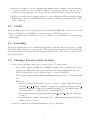
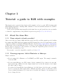
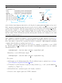
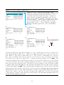
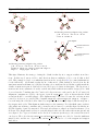
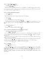
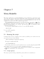
R2R version 1.0.1 user manual
Software to speed the depiction of
aesthetic consensus RNA secondary structures
Zasha Weinberg
November 27, 2010
8%
A
A
3%
89%
G
3 nt
R
A
pseudoknot
U R
R
Y R
6 nt
G
C
G C
U R
C G
UA
0-6 nt
A
G R
GU
G
R
R
Y
A
CA
U G
G U
G
AA
C
Y
Y
AG
G C
G C
R
U
A
G
G C
G
Y
R
R
UY
Y
U
G
AAU
CC Y
R
G
G
G C
C GU
G C
5‘
A
C
Y C
Y R
U
A
G Y
C
R
C
Y
A
GA
Y
Y
R Y
U
G
G
U
Y R
U A
U G C U C G AA
G
YYR
G
U GG A A
GRY
C G
0-12 nt
G
YY
C
C
CR
RR
Y
C
G
AU
A
C
C
A
Y
A
R A CC
C
U
R
pseudoknot?
G
A
C
A
C
U
R
U
G
AY
c 2009-2010 by Zasha Weinberg. All rights reserved.
Copyright This software package, including source code and this manual, is distributed freely but without
any warranty under the terms of the GNU General Public License as published by the Free Software
Foundation. This program is distributed in the hope that it will be useful, but WITHOUT ANY
WARRANTY; without even the implied warranty of MERCHANTABILITY or FITNESS FOR A
PARTICULAR PURPOSE. For a copy of the full text of the GNU General Public License, see
www.gnu.org/licenses.
This package includes the following material from other sources:
• The “Squid” library from Infernal version 0.7 by Sean Eddy.
• Free code that is part of the CFSQP package [5], distributed by AEM Design.
• Previously published layouts of RNAs and R2R markup to generate those layouts [13, 16, 14,
15, 12, 9, 11, 6].
1 Introduction
1.1 What does this software do? . .
1.2 What does this software not do?
1.3 Credit . . . . . . . . . . . . . .
1.4 Licensing . . . . . . . . . . . . .
1.5 Changes from previous versions
.
.
.
.
.
.
.
.
.
.
.
.
.
.
.
.
.
.
.
.
.
.
.
.
.
.
.
.
.
.
.
.
.
.
.
.
.
.
.
.
.
.
.
.
.
.
.
.
.
.
.
.
.
.
.
.
.
.
.
.
.
.
.
.
.
.
.
.
.
.
.
.
.
.
.
.
.
.
.
.
.
.
.
.
.
.
.
.
.
.
.
.
.
.
.
.
.
.
.
.
.
.
.
.
.
5
5
5
6
6
6
. . .
. . .
. . .
. . .
. . .
. . .
. . .
. . .
font
. . .
. . .
. . .
.
.
.
.
.
.
.
.
.
.
.
.
.
.
.
.
.
.
.
.
.
.
.
.
.
.
.
.
.
.
.
.
.
.
.
.
.
.
.
.
.
.
.
.
.
.
.
.
.
.
.
.
.
.
.
.
.
.
.
.
.
.
.
.
.
.
.
.
.
.
.
.
.
.
.
.
.
.
.
.
.
.
.
.
.
.
.
.
.
.
.
.
.
.
.
.
.
.
.
.
.
.
.
.
.
.
.
.
.
.
.
.
.
.
.
.
.
.
.
.
.
.
.
.
.
.
.
.
.
.
.
.
.
.
.
.
.
.
.
.
.
.
.
.
.
.
.
.
.
.
.
.
.
.
.
.
.
.
.
.
.
.
.
.
.
.
.
.
.
.
.
.
.
.
.
.
.
.
.
.
.
.
.
.
.
.
.
.
.
.
.
.
.
.
.
.
.
.
.
.
.
.
.
.
.
.
.
.
.
.
.
.
.
.
.
.
.
.
.
.
.
.
.
.
.
.
.
.
.
.
.
.
.
.
.
.
.
.
.
.
7
7
7
8
8
8
8
8
8
9
9
9
9
3 Tutorial: a guide to R2R with examples
3.1 About the demo files . . . . . . . . . . . . . . . . . . . . . . . . . . . . . . . . . .
3.1.1 Demo output is already provided . . . . . . . . . . . . . . . . . . . . . . .
3.1.2 Drawing programs: Adobe Illustrator or Inkscape . . . . . . . . . . . . . .
3.1.2.1 More technical information . . . . . . . . . . . . . . . . . . . . .
3.1.3 Where the demo files come from . . . . . . . . . . . . . . . . . . . . . . . .
3.2 Example legend to help you with finished drawings . . . . . . . . . . . . . . . . .
3.3 A hypothetical motif to illustrate the basics . . . . . . . . . . . . . . . . . . . . .
3.3.1 Default output of R2R . . . . . . . . . . . . . . . . . . . . . . . . . . . . .
3.3.2 Some typical customizations for consensus diagrams . . . . . . . . . . . . .
3.3.3 Other kinds of drawings: single-molecule and skeleton diagrams . . . . . .
3.4 Common error: “One or more pairs is getting broken by one side getting deleted”
3.5 The place explicit command . . . . . . . . . . . . . . . . . . . . . . . . . . . . . .
3.6 Multistem junctions and turning internal loops . . . . . . . . . . . . . . . . . . . .
3.6.1 Simple circular layout . . . . . . . . . . . . . . . . . . . . . . . . . . . . .
3.6.2 Manual layout of multistem junctions . . . . . . . . . . . . . . . . . . . . .
3.6.3 Automated multistem junction layout with direction constraints . . . . . .
3.6.3.1 Solving multistem junctions can be slow . . . . . . . . . . . . . .
3.6.4 Internal loops . . . . . . . . . . . . . . . . . . . . . . . . . . . . . . . . . .
.
.
.
.
.
.
.
.
.
.
.
.
.
.
.
.
.
.
10
10
10
10
11
11
12
12
12
15
15
17
19
21
21
21
23
27
28
.
.
.
.
.
.
.
.
.
.
.
.
.
.
.
.
.
.
.
.
.
.
.
.
.
.
.
.
.
.
2 Installation
2.1 Platforms on which R2R is known to work
2.2 Decide whether to install CFSQP or not .
2.3 Make 3rd-party tools . . . . . . . . . . . .
2.3.1 Infernal . . . . . . . . . . . . . . .
2.3.2 CFSQP (optional) . . . . . . . . .
2.4 Make R2R . . . . . . . . . . . . . . . . . .
2.4.1 Optionally edit Makefile . . . . . .
2.4.1.1 Optionally enable CFSQP
2.4.1.2 Optionally choose an SVG
2.4.2 Run make . . . . . . . . . . . . . .
2.5 Adobe Reader glitch . . . . . . . . . . . .
2.6 Alignment editor software . . . . . . . . .
1
.
.
.
.
.
.
.
.
.
.
3.7
3.8
Modular structures . . . . . . . . . . . . . . . . . . . . . . . . . . . . . . . . . . . .
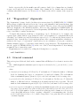
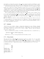
Pseudoknots . . . . . . . . . . . . . . . . . . . . . . . . . . . . . . . . . . . . . . . .
3.8.1 A note on the representation of pseudoknotted secondary structures within
Stockholm files . . . . . . . . . . . . . . . . . . . . . . . . . . . . . . . . . .
3.8.2 Pseudoknots drawn with callouts . . . . . . . . . . . . . . . . . . . . . . . .
3.8.3 Pseudoknots drawn with in-line style . . . . . . . . . . . . . . . . . . . . . .
3.9 Preparing presentations using projectors . . . . . . . . . . . . . . . . . . . . . . . .
3.10 How to draw GOLLD RNA from R2R output . . . . . . . . . . . . . . . . . . . . .
3.11 Making the demo output files . . . . . . . . . . . . . . . . . . . . . . . . . . . . . .
4 Reference: automated inference of nucleotide conservation levels
4.1 Recommended command . . . . . . . . . . . . . . . . . . . . . . . . .
4.2 “Fragmentary” alignments . . . . . . . . . . . . . . . . . . . . . . . .
4.3 General command . . . . . . . . . . . . . . . . . . . . . . . . . . . . .
4.4 Output of R2R for the consensus . . . . . . . . . . . . . . . . . . . .
4.5 Generating your own alignment consensus, bypassing R2R . . . . . .
.
.
.
.
.
.
.
.
.
.
.
.
.
.
.
.
.
.
.
.
5 Reference: drawing
5.1 Running R2R . . . . . . . . . . . . . . . . . . . . . . . . . . . . . . . . . . .
5.2 About the Stockholm file format . . . . . . . . . . . . . . . . . . . . . . . . .
5.2.1 A note on R2R’s representation of consensus secondary structures . .
5.3 R2R “drawing units” . . . . . . . . . . . . . . . . . . . . . . . . . . . . . . .
5.4 Data types in R2R . . . . . . . . . . . . . . . . . . . . . . . . . . . . . . . .
5.4.1 hitId . . . . . . . . . . . . . . . . . . . . . . . . . . . . . . . . . . . .
5.4.2 Distances . . . . . . . . . . . . . . . . . . . . . . . . . . . . . . . . .
5.4.3 Angles . . . . . . . . . . . . . . . . . . . . . . . . . . . . . . . . . . .
5.4.4 Measurements (length/width/size) . . . . . . . . . . . . . . . . . . .
5.4.5 Colors . . . . . . . . . . . . . . . . . . . . . . . . . . . . . . . . . . .
5.5 .r2r meta file . . . . . . . . . . . . . . . . . . . . . . . . . . . . . . . . . . .
5.5.1 Defines . . . . . . . . . . . . . . . . . . . . . . . . . . . . . . . . . . .
5.5.2 SetDrawingParam . . . . . . . . . . . . . . . . . . . . . . . . . . . . .
5.5.3 Oneseq mode . . . . . . . . . . . . . . . . . . . . . . . . . . . . . . .
5.5.4 Skeleton mode . . . . . . . . . . . . . . . . . . . . . . . . . . . . . . .
5.5.5 Entropy mode . . . . . . . . . . . . . . . . . . . . . . . . . . . . . . .
5.5.6 Cleavage diagrams . . . . . . . . . . . . . . . . . . . . . . . . . . . .
5.5.6.1 Multiple drawings of the same RNA molecule . . . . . . . .
5.6 The R2R solver cache . . . . . . . . . . . . . . . . . . . . . . . . . . . . . . .
5.7 Labels . . . . . . . . . . . . . . . . . . . . . . . . . . . . . . . . . . . . . . .
5.7.1 Main labels . . . . . . . . . . . . . . . . . . . . . . . . . . . . . . . .
5.7.2 Extra named label lines . . . . . . . . . . . . . . . . . . . . . . . . .
5.7.3 Sequence-specific (optional) . . . . . . . . . . . . . . . . . . . . . . .
5.7.4 SS cons . . . . . . . . . . . . . . . . . . . . . . . . . . . . . . . . . .
5.7.5 Using labels and special labels . . . . . . . . . . . . . . . . . . . . . .
5.8 R2R commands . . . . . . . . . . . . . . . . . . . . . . . . . . . . . . . . . .
5.8.1 Conditional commands . . . . . . . . . . . . . . . . . . . . . . . . . .
5.8.1.1 Define symbols . . . . . . . . . . . . . . . . . . . . . . . . .
5.8.1.2 Commands that apply to only a consensus or single-molecule
5.8.1.3 Other kinds of conditional commands . . . . . . . . . . . . .
2
.
.
.
.
.
.
.
.
.
.
.
.
.
.
.
.
.
.
.
.
29
31
31
31
33
35
35
35
37
37
38
38
39
40
41
. . . . 41
. . . . 41
. . . . 42
. . . . 42
. . . . 43
. . . . 43
. . . . 43
. . . . 43
. . . . 43
. . . . 43
. . . . 44
. . . . 44
. . . . 44
. . . . 48
. . . . 48
. . . . 48
. . . . 48
. . . . 49
. . . . 49
. . . . 50
. . . . 50
. . . . 51
. . . . 51
. . . . 51
. . . . 51
. . . . 52
. . . . 52
. . . . 52
drawing 53
. . . . 53
5.8.2
Turning and positioning . . . . . . . . . . . . . . . . . . . . . . . . . . . . .
5.8.2.1 Set dir . . . . . . . . . . . . . . . . . . . . . . . . . . . . . . . . . .
5.8.2.2 Laying out arbitrary units like a bulge . . . . . . . . . . . . . . . .
5.8.2.3 Layout single-stranded loops along a straight line, instead of circle .
5.8.2.4 turn ss . . . . . . . . . . . . . . . . . . . . . . . . . . . . . . . . . .
5.8.2.5 turn stem at internal . . . . . . . . . . . . . . . . . . . . . . . . . .
5.8.2.6 place explicit . . . . . . . . . . . . . . . . . . . . . . . . . . . . . .
5.8.3 Layout of multi-stem junctions . . . . . . . . . . . . . . . . . . . . . . . . .
5.8.3.1 Manual layout . . . . . . . . . . . . . . . . . . . . . . . . . . . . .
5.8.3.2 Multi-stem junctions: automatic circular layout . . . . . . . . . . .
5.8.4 Changing layout of secondary structure . . . . . . . . . . . . . . . . . . . . .
5.8.4.1 depair . . . . . . . . . . . . . . . . . . . . . . . . . . . . . . . . . .
5.8.4.2 Internal loop to bulges . . . . . . . . . . . . . . . . . . . . . . . . .
5.8.4.3 Ignore pseudoknots entirely . . . . . . . . . . . . . . . . . . . . . .
5.8.4.4 Ignoring pseudoknots for the purposes of layout . . . . . . . . . . .
5.8.4.5 subst ss . . . . . . . . . . . . . . . . . . . . . . . . . . . . . . . . .
5.8.4.6 merge ss . . . . . . . . . . . . . . . . . . . . . . . . . . . . . . . . .
5.8.5 variable-length regions . . . . . . . . . . . . . . . . . . . . . . . . . . . . . .
5.8.5.1 var hairpin . . . . . . . . . . . . . . . . . . . . . . . . . . . . . . .
5.8.5.2 var term loop . . . . . . . . . . . . . . . . . . . . . . . . . . . . . .
5.8.5.3 Variable-length backbone . . . . . . . . . . . . . . . . . . . . . . .
5.8.5.4 var stem . . . . . . . . . . . . . . . . . . . . . . . . . . . . . . . . .
5.8.6 Annotation . . . . . . . . . . . . . . . . . . . . . . . . . . . . . . . . . . . .
5.8.6.1 Tick labels (like the nucleotide numbering in cleavage diagrams) . .
5.8.6.2 nobpannot . . . . . . . . . . . . . . . . . . . . . . . . . . . . . . . .
5.8.6.3 Pseudo-bold fonts . . . . . . . . . . . . . . . . . . . . . . . . . . .
5.8.6.4 Changing nucleotide colors . . . . . . . . . . . . . . . . . . . . . . .
5.8.6.5 Circling nucleotides . . . . . . . . . . . . . . . . . . . . . . . . . . .
5.8.6.6 Boxing nucleotides . . . . . . . . . . . . . . . . . . . . . . . . . . .
5.8.6.7 Outlining/inlining nucleotides . . . . . . . . . . . . . . . . . . . . .
5.8.6.8 Boxing a set of nucleotides . . . . . . . . . . . . . . . . . . . . . . .
5.8.6.9 Shading nucleotides along the backbone . . . . . . . . . . . . . . .
5.8.6.10 Outlining a stretch of nucleotides around both ends . . . . . . . . .
5.8.6.11 Shading the backbone in skeleton drawings . . . . . . . . . . . . . .
5.8.6.12 Drawing circles associated with loops . . . . . . . . . . . . . . . . .
5.8.6.13 Drawing direct lines between consecutive nucleotides. . . . . . . . .
5.8.7 Miscellaneous . . . . . . . . . . . . . . . . . . . . . . . . . . . . . . . . . . .
5.8.7.1 Override default parameters for drawing . . . . . . . . . . . . . . .
5.8.7.2 No 5 prime label . . . . . . . . . . . . . . . . . . . . . . . . . . . .
5.8.7.3 Adding G for transcription . . . . . . . . . . . . . . . . . . . . . .
5.8.7.4 Keeping gap columns in the drawing . . . . . . . . . . . . . . . . .
5.8.7.5 Breaking pairs . . . . . . . . . . . . . . . . . . . . . . . . . . . . .
5.8.7.6 Deleting columns using an explicit command . . . . . . . . . . . . .
5.9 Troubleshooting . . . . . . . . . . . . . . . . . . . . . . . . . . . . . . . . . . . . . .
5.10 Text output of r2r useful in debugging . . . . . . . . . . . . . . . . . . . . . . . . .
5.10.1 Start/end of file . . . . . . . . . . . . . . . . . . . . . . . . . . . . . . . . . .
5.10.2 consensus lines and “raw” coordinates . . . . . . . . . . . . . . . . . . . . .
5.10.3 Preliminary secondary structure drawing units . . . . . . . . . . . . . . . . .
3
54
54
54
54
54
55
55
55
55
57
62
62
63
63
63
63
64
64
64
64
64
65
65
65
66
66
66
66
66
66
67
67
67
68
68
68
68
68
68
69
69
69
69
69
70
70
70
70
5.10.4 place explicit links . . . . . . . . . . . . . . . . . . . . . . . . . . . . . . . .
5.10.5 Selecting the place explicit commands . . . . . . . . . . . . . . . . . . . . . .
6 Reference: modular structures
6.1 Sub-families . . . . . . . . . . . . . . . . . . . . . . . .
6.2 Using SelectSubFamilyFromStockholm.pl . . . . . .
6.2.1 Command line . . . . . . . . . . . . . . . . . . .
6.2.2 How to define predicates . . . . . . . . . . . . .
6.2.2.1 Regex predicates . . . . . . . . . . . .
6.2.2.2 Perl predicates . . . . . . . . . . . . .
6.2.3 How the file is modified by applying a predicate
.
.
.
.
.
.
.
.
.
.
.
.
.
.
.
.
.
.
.
.
.
.
.
.
.
.
.
.
.
.
.
.
.
.
.
.
.
.
.
.
.
.
.
.
.
.
.
.
.
7 Meta-Makefile
7.1 Running the script . . . . . . . . . . . . . . . . . . . . . . . . . . .
7.1.1 Script options . . . . . . . . . . . . . . . . . . . . . . . . . .
7.1.2 Makefile targets . . . . . . . . . . . . . . . . . . . . . . . . .
7.2 Additional markup for .sto files . . . . . . . . . . . . . . . . . . . .
7.2.1 Implicit rules . . . . . . . . . . . . . . . . . . . . . . . . . .
7.2.2 Explicit rules . . . . . . . . . . . . . . . . . . . . . . . . . .
7.2.2.1 Oneseq . . . . . . . . . . . . . . . . . . . . . . . .
7.2.2.2 Skeleton . . . . . . . . . . . . . . . . . . . . . . . .
7.2.2.3 Defines for consensus diagrams . . . . . . . . . . .
7.2.2.4 Using define directive with modular structure . . .
7.2.2.5 Oneseq for a predicate defining a modular structure
8 R2R source code
8.1 Summary of C++ and Perl source code files
8.2 Other information . . . . . . . . . . . . . . .
8.2.1 Overall layout of RNA . . . . . . . .
8.2.2 Inferring a path for the backbone . .
4
.
.
.
.
.
.
.
.
.
.
.
.
.
.
.
.
.
.
.
.
.
.
.
.
.
.
.
.
.
.
.
.
.
.
.
.
.
.
.
.
.
.
.
.
.
.
.
.
.
.
.
.
.
.
.
.
.
.
.
.
.
.
.
.
.
.
.
.
.
.
.
.
.
.
.
.
.
.
.
.
.
.
.
.
.
.
.
.
.
.
.
.
.
.
.
.
.
.
.
.
.
.
.
.
.
.
.
.
.
.
.
.
.
.
.
.
.
.
.
.
.
.
.
.
.
.
.
.
.
.
.
.
.
.
.
.
.
.
.
.
.
.
.
.
.
.
.
.
.
.
.
.
.
.
.
.
.
.
.
.
.
.
.
.
.
.
.
.
.
.
.
.
.
.
.
.
.
.
.
.
.
.
.
.
.
.
.
.
.
.
.
.
.
.
.
.
.
.
.
.
.
.
.
.
.
.
.
.
.
.
.
.
.
.
.
.
.
.
.
.
.
.
.
.
.
.
.
.
71
72
.
.
.
.
.
.
.
73
73
73
73
73
74
74
75
.
.
.
.
.
.
.
.
.
.
.
76
76
76
77
78
78
78
78
78
78
78
79
.
.
.
.
80
80
82
82
82
Chapter 1
Introduction
1.1
What does this software do?
For a full description of this software, please read the paper by Zasha Weinberg and Ronald R.
Breaker entitled “R2R—software to speed the depiction of aesthetic consensus RNA secondary
structures”.
Briefly, this software is designed to speed the drawing of RNA secondary structure consensus
diagrams, which show the conserved features within a set of related RNAs. The software also
supports drawing of single RNA molecules, although this is not the emphasis. To make RNA
drawings, many biologists use general-purpose software such as Adobe Illustrator, at great cost
in time and risk of errors. However, this strategy produces the highest-quality of drawings. R2R
is designed to allow the user to achieve this highest-quality drawing, while taking much less time
than the manual solution. Because of this goal, R2R imposes more work on the user than highly
automated solutions, and the current version of R2R is aimed at bioinformaticians, or biologists
with some familiarity with UNIX-like command line tools.
I have used R2R to draw over 100 RNA consensus diagrams. These drawings are made available
as “demo” files (see Chapter 3).
1.2
What does this software not do?
R2R has some important limitations:
• R2R does not fully automate determination of a layout. Although its default layouts will get
you closer to an ideal layout and it has functions to assist in determining layouts of multistem
junctions, R2R does not solve the problem of determining an overall layout. No currently
available computer algorithm can determine an ideal layout that is comparable in quality to
the best layouts found by a person. Therefore, R2R assumes that a user will optimize the
layout and tell R2R what to do.
• R2R does not have a graphical user interface. As noted above, R2R is aimed at bioinformaticians. Successful use of R2R will likely require some general familiarity with the UNIX
command line, and comfort with command-driven programs. Because of the lack of a graphical
user interface, R2R might have a significant learning curve. So, if you just want to draw one
RNA, it might be most efficient to go straight to Adobe Illustrator, Inkscape or CorelDRAW.
5
• R2R is not designed to produce drawings that illustrate many elements of tertiary structure,
or whose layouts are based on atomic-resolution 3-D structures. R2R is only intended to
create more abstract layouts of secondary structure that reflect Watson-Crick base pairing.
• R2R is not a fully general drawing program, or even a fully general RNA-drawing program.
R2R should be used in combination with general-purpose drawing programs like Adobe Illustrator or Inkscape.
1.3
Credit
If you use R2R, please cite the paper Weinberg Z, Breaker RR (2010) R2R—software to speed the
depiction of aesthetic consensus RNA secondary structures, BMC Bioinformatics.
If you distribute R2R or derivatives of it, please continue to credit Infernal, as on the first page
of this manual.
1.4
Licensing
The files in the main directory (documentation), the src and the demo subdirectories are copyright
2009-2010 by Zasha Weinberg, except as noted. The entire package is distributed freely but without
any warranty whatsoever under the GNU General Public License. For details, see http://www.
gnu.org/licenses.
1.5
Changes from previous versions
• Version 1.0.1 (distributed with revised version of paper, November 2010)
– Added demo: demo/c-di-GMP-II/c-di-GMP-II-update.sto (re-drawing based on new
sequences, for Wikipedia article), also some files in the demo/pedagogical directory.
– Added Additional files 3 and 4 from the paper to software distribution.
– Added feature: indicateOneseqWobblesAndNonCanonicals added as a drawing parameter.
– Fixed bugs:
∗ Fixed a problem when internal loops are converted to bulges (explicitly using the
internal loop to bulges command, or implicitly by applying a bulge or place explicit command to a nucleotide within the internal loop), and when the user did
not specify what to do with both sides of the internal loop.
∗ Fixed various issues with applying the multistem junction circular command to
30 bulges.
∗ Formatting issues with the user manual. The --GSC-weighted-consensus flag was
explained in more detail.
• Version 1.0 (distributed with initial submission of paper, July 2010)
6
Chapter 2
Installation
Installation essentially means making the executable file r2r.
2.1
Platforms on which R2R is known to work
Building of R2R has only been tested with the gcc compiler suite (http://gcc.gnu.org). To ensure
compatibility, you will need the GNU C compiler (which provides the gcc command) and the GNU
C++ compiler (which provides the g++ command).
R2R has been tested on the following platforms:
• gcc version 3.4.4 under Cygwin 1.5.25 (32-bit) on Windows XP.
• gcc version 4.3.4 under Cygwin 1.7.1 (32-bit) on Windows 7.
• gcc version 4.1.2 under Ret Hat Linux running Linux kernel 2.6.18 (64-bit).
• gcc version 3.3 under MacOS’s Darwin version 8.8.0 (32-bit).
I presume that R2R will work on gcc version 3 or higher on Cygwin, Linux or MacOS Darwin.
R2R is known to produce output that can be used with Adobe Illustrator CS on Windows XP,
Inkscape 0.46 on Windows XP and CorelDRAW Graphics Suite X4 on Windows Vista. I presume,
however, that the output will work on any version of these programs, at least with appropriate
setting of fonts (see below).
2.2
Decide whether to install CFSQP or not
R2R implements multiple methods to find a good layout for multistem junctions. Some automated
solutions require software that can solve non-linear optimization problems. You have two options:
• Option 1: Do not install a solver. (This is the default.)
Advantage: easiest installation.
Disadvantage: some functionality for multistem junctions won’t work.
If you do not use the multistem junction non-linear solvers, there is no disadvantage to this
option. However, the R2R commands multistem junction circular solver, multistem junction bulgecircley solver and multistem junction bulgecircleynormals solver will
not work; R2R will report an error.
7
• Option 2: Install CFSQP.
Advantage: all functionality will work.
Disadvantage: CFSQP must be requested from AEM Design, which requires additional time.
CFSQP allows for all the automated layout schemes for multistem junctions. However, CFSQP must be requested from AEM Design (see below), and is not available for commercial
purposes. Unfortunately, I am not permitted to distribute CFSQP with R2R.
2.3
Make 3rd-party tools
2.3.1
Infernal
R2R uses the Squid library that was distributed with an older version of the Eddy Lab’s “Infernal”
software. I have removed much of the code that is not used by R2R. The remaining subset of
Infernal is in the subdirectory NotByZasha/infernal-0.7. (The full Infernal package, along with
more recent releases, is available from http://infernal.janelia.org.)
To build the squid part of Infernal, run the following three commands:
cd NotByZasha/infernal-0.7
./configure
make
Note:
• No “installation” of Infernal is necessary. R2R uses only the infernal-0.7/squid/libsquid.a
file.
• You must use Infernal version 0.7. More recent versions of the Infernal software might not
work, and Infernal version 1.0 is guaranteed to fail.
2.3.2
CFSQP (optional)
If you want to use the CFSQP solver, you must request the proprietary file cfsqp.c. Go to
http://www.aemdesign.com/ or http://www.ece.umd.edu/Newsletter/vol5 no1/fsqp.htm or
Google for CFSQP. (The contact has changed recently.) Put the file cfsqp.c into the R2R directory
NotByZasha/cfsqp. Then cd into this directory and run make.
2.4
Make R2R
2.4.1
Optionally edit Makefile
2.4.1.1
Optionally enable CFSQP
R2R is configured by default to disable CFSQP. To enable CFSQP, go within the src directory, open
the file Makefile in a text editor such as emacs or vi. Remove the line that reads DISABLE CFSQP=1.
8
2.4.1.2
Optionally choose an SVG font
If you intend to use Adobe Illustrator or CorelDRAW, you can use the PDF (Adobe Acrobat)
output of R2R. In this case, you do not need to set a font.
If you intend to use Inkscape, you should use the SVG output of R2R, since Inkscape is not
reliable when importing PDFs generated by R2R. By default, R2R is set up to produce SVG output
using the “Bitstream Vera Sans” font, which is freely available (http://www.gnome.org/fonts/)
and might already be installed on your system. If, however, Inkscape is not mapping your font
correctly, you can get R2R to generate SVG files that reference a different font.
(Note: it might be easiest to skip this step initially, and change the font later if there are
problems in Inkscape. To change the font later, modify the Makefile as described below, then run
make clean, then run make.)
To change this font, open the file src/Makefile in a text editor and change the definition of the
FONT CFLAGS variable. (Search for “FONT CFLAGS”, and read the comment immediately above
this line.)
Note: R2R is internally hardcoded with font geometry that is appropriate to Helvetica, Arial,
Bitstream Vera or DejaVu fonts. These fonts have similar sizes to each other. If you use fonts whose
symbols have significantly different sizes, nucleotides will not be positioned correctly.
2.4.2
Run make
Finally, run go into the src directory and run make.
Note: the first file, ParseOneStockholm.cpp might take a surprising amount of time to compile.
This is normal. The file is just very large.
If everything works, there will be an executable file named r2r within the src directory.
2.5
Adobe Reader glitch
This section describes a potential problem when viewing PDF output with Adobe Reader. With recent versions of Adobe Reader and certain computer configurations, circles and arcs appear jagged—
more like polygons. To prevent this, while running Adobe Reader, select “Preferences” under the
“Edit” menu. Within the category “Page Display”, uncheck “Use 2D graphics acceleration” and
make sure that “Smooth line art” is checked.
2.6
Alignment editor software
R2R’s input is based upon multiple-sequence alignments that are stored in Stockholm-format files.
Although these files can be edited in any text editor, some programs are customized for them. One
example is RALEE [4], which is a set of macros for the Emacs text editor.
9
Chapter 3
Tutorial: a guide to R2R with examples
This chapter gives a practical introduction with examples on how to create RNA drawings with
R2R. Example input files containing R2R commands to draw various RNA structures are available
in the demo subdirectory.
Credit: the Stockholm-format input files in the demo directory and its subdirectories are similar
or identical to supplementary data published in previous reports [13, 15, 9, 12, 16, 14, 6].
3.1
About the demo files
3.1.1
Demo output is already provided
I have created the raw output of R2R when run on the demo files, and this output is provided within
the output-pdf (PDF format) and output-svg (SVG format) directories. If you just want to see the
output, I recommend opening the PDF files using Adobe Reader (http://get.adobe.com/reader),
as this should work on any platform. (Note: if circles look very unsmooth when viewed in Adobe
Reader, please see Section 2.5.) If you want to try editing the output files, please see Section 3.1.2
(next) to find out which files to use.
If you want to create the output files yourself, see Section 3.11.
3.1.2
Drawing programs: Adobe Illustrator or Inkscape
Simple conclusion:
• If you’re using Adobe Illustrator or CorelDRAW, use PDF output. The example commands
below use PDF.
• If you’re using Inkscape, use SVG output. In the commands below, wherever it says pdf,
instead write svg. (R2R decides the output format based on the file extension of its output
file, either .pdf or .svg.)
If you have problem with the fonts in Inkscape (or if the letters don’t show up), you might
need to re-create the SVG output with a different font name. Please see the next section
(“more technical information”) to learn more about this, and Chapter 2 for information on
how to change the font.
10
3.1.2.1
More technical information
R2R will generate valid PDF and SVG files as output. In principle, any program should be able
to read them. However, I am exploiting the fact that the Helvetica font is built in to PDF. Some
versions of Inkscape will not render any text using PDFs built by R2R because they don’t have the
Helvetica font.
Therefore, R2R can create SVG output, which is Inkscape’s native file format. The SVG output
uses the Bitstream Vera Sans font, which is similar to Helvetica and to Inkscape’s default font.
(Meanwhile, at least on Windows, Illustrator will substitute Arial, which is similar.)
Note: in principle you can substitute other fonts, even by creating scripts to edit SVG output.
However, R2R knows the heights and width of font symbols, which is uses for its layout. Thus, for
example, if you use a narrower font, the spacing might not be appropriate.
3.1.3
Where the demo files come from
Files within the demo directory were made to support this user manual. Most are based on previously
drawn RNAs. RNA drawings derived from previous studies are organized into subdirectories. The
subdirectories and relevant citations are as follows:
• demo/22 (Weinberg et al., 2007) [13] and (Sudarsan et al., 2008) [11].
• demo/104 (Weinberg et al., 2010) [16].
• demo/exceptional (Weinberg et al., 2009) [14]. Note:
– The RNAs depicted in Supplementary Figure 11 of this paper are primarily described
in the (Weinberg et al., 2010) paper [16], and are therefore found within the demo/104
directory.
– The drawing of GOLLD RNA is somewhat complicated by different degrees of conservation of the structural elements. For instructions on reproducing the drawing of GOLLD
RNA in Fig. 2a, see Section 3.10.
Also, a careful look at Fig. 2a in Nature will reveal that many nucleotides are slightly
misaligned. The reason is that the R2R drawings in this case were done using Adobe’s
Myriad font, which is narrower than Helvetica. The journal changed the font, but did
not realign the nucleotide letters. The output of R2R is always aligned correctly.
– The HEARO RNA “skeleton” drawing in Figure 3b was not drawn with R2R. However,
an R2R drawing of this style is included. Figure 3b was drawn before I had implemented
skeleton drawings in R2R.
• demo/c-di-GMP-II (Lee et al., 2010) [6]
• demo/Moco (Regulski et al., 2008) [9]. (New drawing, based on original layout.)
• demo/SAH (Wang et al., 2008) [12]. (New drawing, based on original layout.)
• demo/SAM-IV (Weinberg et al., 2008) [15].
• demo/hammerhead (Perreault et al., 2010) [7]
• demo/additional Drawings of RNAs that were identified by other groups. The tRNA drawing
is based on the standard layout.
11
• demo/pedagogical Some drawings I did to explain issues in RNA drawing to non-biologists,
or for the R2R paper.
Figures within each directory are organized by motif name. Thus, for example, in (Weinberg
et al., 2009) [14], Figure 2a is a consensus diagram of GOLLD RNA. This corresponds to the files
demo/exceptional/GOLLD.sto and demo/exceptional/GOLLD.r2r meta. If you run r2r on these
files, the output will be found in output-pdf/GOLLD.pdf or output-svg/GOLLD.svg. Similarly,
Supplementary Figure 1 of the same previous publication contains a skeleton diagram of GOLLD
RNA, Supplementary Figure 2 has an expanded consensus diagram and Supplementary Figure 3
holds a different skeleton diagram and a drawing of certain parts of the L. brevis GOLLD RNA.
All these figures are generated from the same files, and R2R output used for this will also appear
in output-pdf/GOLLD.pdf or output-svg/GOLLD.svg.
3.2
Example legend to help you with finished drawings
To create a finished drawing for a published figure, a legend is necessary to explain the annotations.
We have created generic annotations usable for a legend:
• Use the file demo/Additional-file-3.pdf for PDF format that can be imported into Adobe
Illustrator or CorelDRAW.
• Use the file demo/Additional-file-4.svg for SVG format that can be imported into Inkscape.
3.3
A hypothetical motif to illustrate the basics
Now the actual tutorial begins.
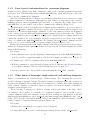
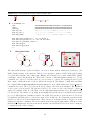
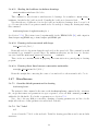
3.3.1
Default output of R2R
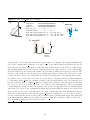
Figure 3.1 shows a simple alignment, and R2R’s drawing of the consensus of the alignment. Elements
of the Stockholm-format alignment file are illustrated.
The drawing was made by running the following commands within the demo directory. (Actually,
I really just ran make, which reads the Makefile in that directory to run these commands. If you’re
familiar with the UNIX make command, and you’re going to make many drawings, you might want
to read Chapter 7 after reading this tutorial.)
First, in order to draw the consensus structure, we must first run a command to calculate it.
We calculate the alignment’s consensus (Figure 3.1D) using the following command line (note: the
following command should be one line, but was split into two lines for typesetting):
commandprompt$ ../src/r2r --GSC-weighted-consensus demo1.sto
(continued)
intermediate/demo1.cons.sto 3 0.97 0.9 0.75 4 0.97 0.9 0.75 0.5 0.1
(All commands in this section should be run within the demo directory that is part of the R2R
distribution.)
The general form of this command is
commandprompt$ ../src/r2r --GSC-weighted-consensus input-file.sto
output-file.sto 3 0.97 0.9 0.75 4 0.97 0.9 0.75 0.5 0.1
12
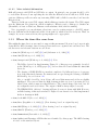
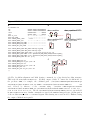
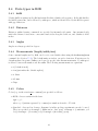
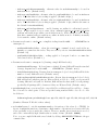
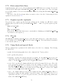
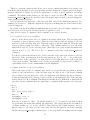
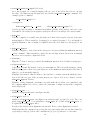
Figure 3.1 demo1: A simple alignment and R2R drawing
A
B
# STOCKHOLM 1.0
human
ACACGCGAAA.GCGCAA.CAAACGUGCACGG
chimp
GAAUGUGAAAAACACCA.CUCUUGAGGACCU
bigfoot
UUGAG.UUCG..CUCGUUUUCUCGAGUACAC
#=GC SS_cons ...<<<.....>>>....<<....>>.....
//
This identifies the line as
being the secondary
structure consensus.
R
G C
5´
R
C
Y
G
Y G
AC
All stockhom files begin
with “# STOCKHOLM 1.0”
C
A “hit id”, which identifies
this sequence by the
name “chimp”.
demo1
A gap within this sequence.
# STOCKHOLM 1.0
human
ACACGCGAAA.GCGCAA.CAAACGUGCACGG
chimp
GAAUGUGAAAAACACCA.CUCUUGAGGACCU
bigfoot
UUGAG.UUCG..CUCGUUUUCUCGAGUACAC
#=GC SS_cons ...<<<.....>>>....<<....>>.....
An unpaired
pair
pair
//
column
pair
pair
pair
All stockhom files end
with “//”.
This column is not represented in the
drawing in part B, because it is mostly gaps.
D
The consensus line
inferred by R2R. ‘n’
corresponds to a
circle in the
diagrams. ‘-’ is a gap.
The numbers below
define the degree of
conservation (colors
in the diagrams).
# STOCKHOLM 1.0
human
chimp
bigfoot
#=GC SS_cons
#=GC cons
#=GC conss
#=GC cov_SS_cons
//
ACACGCGAAA.GCGCAA.CAAACGUGCACGG
GAAUGUGAAAAACACCA.CUCUUGAGGACCU
UUGAG.UUCG..CUCGUUUUCUCGAGUACAC
...<<<.....>>>....<<....>>.....
nnRnGnnnnR-nCnCnn-YnnnYGnGnACnn
1111141111041111101111111111111
...202.....202....12....21.....
Covariation
E
No mutation
observed
This column is classified
as a gap by R2R.
Compatible
mutation
intermediate/demo1.cons.sto
(A) A minimal Stockholm-format alignment of a hypothetical RNA motif. This is the file demo/demo1.sto.
(B) The raw output of R2R when run on the alignment in part A. Note that the text “demo1” is part
of R2R’s raw output. (C) Annotations of the alignment file. (D) The Stockholm-format alignment file
generated by R2R (with the --GSC-weighted-consensus flag) that has information on the consensus of
the demo1 motif. (Some minor changes were made to improve readability.) Note that it is not necessary to
understand the information in this file, because the file is simply used by R2R to produce its final output.
The way in which R2R calculates consensus diagrams, and the meanings of the colors and symbols is
explained in the research paper, as well as in Chapter 4. (E) The contents of the file demo/demo.r2r meta.
In this case, the file simply lists the name of input file used to draw the consensus.
13
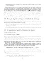
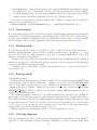
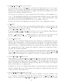
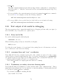
Figure 3.2 demo1-ii: Some annotation for the consensus diagram
A
B
# STOCKHOLM 1.0
human
ACACGCGAAA.GCGCAA.CAAACGUGCACGG
chimp
GAAUGUGAAAAACACCA.CUCUUGAGGACCU
bigfoot
UUGAG.UUCG..CUCGUUUUCUCGAGUACAC
#=GC SS_cons
...<<<.....>>>....<<....>>.....
#=GC R2R_LABEL --...<.....>...1.2.....L.....-#=GF R2R var_hairpin < >
dash
#=GF R2R var_backbone_range 1 2
character
#=GF R2R tick_label L magic G
//
label references
space character
var_hairpin
demo1-ii
tick_label
Y
G
G C
5´ R
C
Y G
2-3 nt
magic G
AC
var_backbone_range
(A) Stockholm-format alignment that includes a labeling line (beginning #=GF R2R LABEL) and associated
R2R commands (beginning #=GF R2R). Annotations in blue show how R2R commands are associated with
a symbol in the labeling line. Annotations also mark the special dash symbol in the #=GC R2R LABEL line
that causes the column to be deleted from R2R’s drawing. Also it is important to note that a single space
character separates all elements of R2R commands. (This text is identical to the file demo/demo1-ii.sto.)
(B) Raw output of R2R, with annotation (in blue) showing what elements of the drawing were the result
of the R2R commands in part A.
This command is explained in Chapter 4, and the parameters are fully explained in Section 4.3.
Also, while it is necessary to generate consensus information so that R2R can draw it, users can write
their own routine to generate the consensus data instead of using the --GSC-weighted-consensus
command; this alternative is explained in Section 4.5.
Given the consensus data generated by the previous command, we run R2R to create a PDF
file. The file demo1.r2r meta simply gives the path of intermediate/demo1.cons.sto, which is
what R2R will use to draw.
commandprompt$ ../src/r2r demo1.r2r meta output/demo1.pdf
Alternately, to create SVG-format output:
commandprompt$ ../src/r2r demo1.r2r meta output/demo1.svg
Key points:
• R2R inputs are Stockholm-format files. The Stockholm format is explained more at http:
//en.wikipedia.org/wiki/Stockholm format.
• Consensus secondary structure is expressed using brackets (e.g., < and >) in the #=GC SS cons line (e.g., Figure 3.1).
• R2R will infer the consensus sequence and classify covariation.
• Creation of the output requires two UNIX commands.
14
3.3.2
Some typical customizations for consensus diagrams
In this section we will use some R2R commands to improve the consensus diagram drawn in the
previous section. This will entail adding an #=GC R2R LABEL line, which will allow us to label and
refer to specific columns in the alignment.
The demo1 drawing in Figure 3.1B has 50 and 30 flanking regions that are not conserved according
to R2R’s definition of conservation. Although it is often desirable to keep such poorly conserved
flanking regions in curated alignments, they add little to a diagram. By adding dashes to the
R2R LABEL line, we cause R2R to remove those columns in the output (see Figure 3.2).
The first hairpin of the demo1 motif varies in length, and its terminal loop is poorly conserved.
The R2R var hairpin command allows us to replace part of the hairpin with an abstract representation of a variable-length hairpin. Similarly, a part of the junction between the hairpins is
poorly conserved, and the R2R var backbone range command replaces this with a line. The line
is annotated with the range in the number of nucleotides contained in those columns, which is automatically calculated. For both commands, the range is represented by two labels, each of which
refer to a column in the #=GC R2R LABEL line. For example, the var hairpin command used the
labels < and >, each of which refers to a specific column, as shown (Figure 3.2A).
Finally, the drawing uses the tick label command, which labels a specific nucleotide position.
In this case, I imagined that a particular G nucleotide has a special biochemical significance in this
fictitious RNA structure.
Key points:
• R2R commands refer to specific alignment columns using labels, in the #=GC R2R LABEL line.
It is also possible to expand the number of labels beyond simply one symbol (see Section 5.7).
• Columns can be deleted by putting dashes in the #=GC R2R LABEL line.
• R2R has commands to represent variable-length regions of different sorts. For more information on R2R commands related to variable-length regions see Section 5.8.5.
• Specific positions can be labeled with a tick mark using the tick label command.
3.3.3
Other kinds of drawings: single-molecule and skeleton diagrams
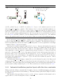
Figure 3.3 demonstrates two additional types of R2R drawings. The .r2r meta file is needed to
specify both kinds of alternate drawing. The first is drawing of a single molecule whose sequence is
present in the alignment. Every tenth nucleotide is numbered by default. These kind drawings are
called “oneseq” drawings, because they depict one sequence. A real-world example of this kind of
drawing is given in Figure 3.4A.
The second kind of drawing is a “skeleton” drawing, which is an outline of the shape. Skeleton drawings can be applied to consensus or to individual sequences, and are useful to give a
compact summary of the whole structure. Larger skeleton drawings are demonstrated in the files
demo/exceptional/GOLLD.sto (and .r2r meta) and demo/exceptional/HEARO.sto (and .r2r meta). Those files also demonstrate making scaled-down “thumbnail” skeleton drawings. A more
realistic example of a skeleton drawing is given in Figure 3.4B.
Key points:
• Fields in the .r2r meta file are separated by tab characters.
• A single RNA molecule can be drawn using the oneseq directive in the .r2r meta file.
15
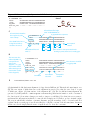
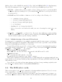
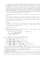
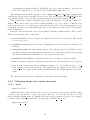
Figure 3.3 demo1-iii: Other kinds of drawings
A
intermediate/demo1-iii.cons.sto
demo1-iii.sto
oneseq bigfoot
intermediate/demo1-iii.cons.sto
B
C
demo1-iii
skeleton-with-pairbonds
tab character
# STOCKHOLM 1.0
human
ACACGCGAAA.GCGCAA.CAAACGUGCACGG
chimp
GAAUGUGAAAAACACCA.CUCUUGAGGACCU
bigfoot
UUGAG.UUCG..CUCGUUUUCUCGAGUACAC
#=GR bigfoot DEL_COLS ..........................----#=GC SS_cons
...<<<.....>>>....<<....>>.....
#=GC R2R_LABEL
--...<.....>...1.2.....Lsssss-#=GC R2R_XLABEL_bf
......UUUU.....................
#=GC R2R_XLABEL_bfl
........U......................
#=GF R2R var_hairpin < >
#=GF R2R var_backbone_range 1 2
#=GF R2R tick_label L magic G
#=GF R2R_oneseq bigfoot outline_nuc bf:U
#=GF R2R_oneseq bigfoot tick_label bfl:U bigfoot UNCG loop
#=GF R2R if_skeleton SetDrawingParam pairBondWidth 0.5pt
#=GF R2R if_skeleton shade_along_backbone s rgb:255,0,0
//
Y
G
G C
5´ R
C
Y G
bigfoot UNCG loop
U C
5´
AC
2-3 nt
demo1-iii bigfoot
U
G
A
U U G
magic G
20
U C
G
C
C 10
U
U
U
C G U U
G
A
G
magic G
demo1-iii skeleton-with-bp
(A) The .r2r meta file name (demo/demo1-iii.r2r meta), which directs R2R to draw a regular consensus
diagram (first line), a single sequence (oneseq) from the “bigfoot” sequence and a skeleton-style schematic
drawing of the consensus. Note that the components in each line are separated by a single tab character.
(B) Stockholm-format alignment. (This text comes from the file demo/demo1-iii.sto. Some irrelevant
markup has been removed.) The two lines beginning #=GF R2R oneseq are only processed within oneseq
mode (i.e., only for the bigfoot sequence in this example). They refer to column labels with alternate
names (bf and bfl) that are introduced using #=GC R2R XLABEL bf and #=GC R2R XLABEL bfl. In the
oneseq case, dashes in the R2R LABEL line are ignored, but dashes in the #=GR bigfoot DEL COLS lines
cause nucleotides to be eliminated from the drawing. The last line, which contains if skeleton, is only
interpreted in skeleton mode, and it overrides a default drawing parameter to set the basepair bond width
to 0.5 points. (C) Raw output of R2R (rearranged to fit the figure space efficiently). From top to bottom
is a standard consensus diagram, a single RNA molecule and a skeleton schematic.
16
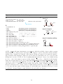
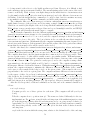
Figure 3.4 Other kinds of drawings illustrated with SAM-IV riboswitches
A
SAM-IV NC_003888.3/2308784-2308334
C C
U
G
G
U
C G
C G 70
C
60 U
G
C G
C G
C G
A
U
A
C G80
40
50 G C C C
G C
G G
G
C
C
A
C
U
G
U
C C
C
C
G G
U G A C A G G
C C
UA
A
C
G
20
G U A
U A C
30
U
G
10
G
5´ G G U U U U U C G A C A
B
SAM-IV skeleton-with-bp
U
C
130 C
C
C
G
A
G
G
G
G
U
C
G
G
A
C
A 120 G
G
A
110
A 90A
G A
C
C G G C A C C U G
A
C
C
A G G U C G U G G A C
A G
100
Examples of oneseq and skeleton drawings using SAM-IV riboswitches [15]. These examples are built from
the files demo/SAM-IV/SAM-IV.sto and demo/SAM-IV/SAM-IV.r2r meta. (A) oneseq drawing of a SAMIV riboswitch from Streptomyces coelicolor annotated with cleavage data from in-line probing experiments
[15]. The annotation of cleavage data used a #=GR ... CLEAVAGE line, as explained in Section 5.5.6.
Note that this is the raw output of R2R, and some adjustment (in Adobe Illustrator or Inkscape) would be
needed to position some of the nucleotide number labels in appropriate places. (B) R2R skeleton drawing
of SAM-IV riboswitch consensus. This layout is the same as in Figure 3.10D, but at a reduced scale.
– For oneseq drawings, nucleotides are removed from the drawing using the DEL COLS
sequence-specific line.
– R2R commands beginning with #=GF R2R oneseq bigfoot are only applied in oneseq
mode for the sequence bigfoot.
• A skeleton-style schematic can be drawn by adding skeleton-with-pairbonds (or skeleton)
in the .r2r meta file. Commands beginning if skeleton are only applied in skeleton mode.
• Drawing parameters can be modified with the SetDrawingParam command. (This command
can also be used in the .r2r meta file.) A list of parameters that can be modified with
SetDrawingParam is provided in Section 5.5.2.
• Lines beginning #=GC R2R XLABEL something can be used to introduce an extra dimension of
labels with the name something. See Section 5.7 for details.
3.4
Common error: “One or more pairs is getting broken
by one side getting deleted”
This sections explains how to handle a common error when using R2R. R2R defines which nucleotide
positions are shown in a consensus based on how frequently they are present in sequences. Sometimes
one nucleotide position involved in a base pair is removed from the consensus while the other is
retained. This can happen with stems that are loosely conserved. When this arises, R2R will report
17
0
1
2
3
4
5
6
7
8
9
10
11
12
13
14
15
16
17
18
19
20
21
22
23
24
25
26
27
28
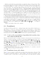
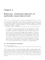
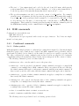
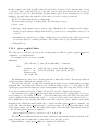
Figure 3.5 demo-breakpair: common error
A
B ERROR: there was a problem drawing motif "demobreakpair": One or more pairs is getting broken by one
side getting deleted (presumably because it's not
conserved), while the other one stays. Because of
generic process (probably RemoveGaps), and not the
result of any specific command. Consider using #=GF
R2R keep allpairs. (Note: another explanation is that
you've used #=GF R2R var_backbone_range on columns
that includes a pair.
(text columns in alignment
[16,25], left=keep,right=chuck, left context=AARC)
# STOCKHOLM 1.0
lemur
AAACUACCCCUAUUGG
blueberry
AAACAUCCCCAU-UGG
smurf
AAGCAACCCCUU-CGG
#=GC SS_cons ..<<<<....>>>>..
//
C
D
E
F # STOCKHOLM 1.0
# STOCKHOLM 1.0
lemur
AAACUACCCCUAUUGG
blueberry
AAACAUCCCCAU-UGG
smurf
AAGCAACCCCUU-CGG
#=GC SS_cons ..<.<<....>>.>..
//
# STOCKHOLM 1.0
lemur
AAACUACCCCUAUUGG
blueberry
AAACAUCCCCAU-UGG
smurf
AAGCAACCCCUU-CGG
#=GC SS_cons
..<<<<....>>>>..
#=GC R2R_LABEL ...p........p...
#=GF R2R depair p
//
# STOCKHOLM 1.0
lemur
AAACUACCCCUAUUGG
blueberry
AAACAUCCCCAU-UGG
smurf
AAGCAACCCCUU-CGG
#=GC SS_cons
..<<<<....>>>>..
#=GC R2R_LABEL ...-........-...
//
lemur
AAACUACCCCUAUUGG
blueberry
AAACAUCCCCAU-UGG
smurf
AAGCAACCCCUU-CGG
#=GC SS_cons
..<<<<....>>>>..
#=GC R2R_LABEL ...p........p...
#=GF R2R keep p
//
G
demo-breakpair-fix4
CC
C C
5´ A A
C
R Y
GG
(A) input Stockholm file (demo/demo-breakpair.sto.err). Column numbers are labeled, with the leftmost column having the number zero. (This is the numbering system used by the text editor program “Emacs”.) (B) output of R2R with an error. The referenced column numbers are circled in
blue. (C) one resolution: since the base pair is not well conserved, remove it from the SS cons line.
(You should only do this if you truly believe, on reflection, that the pairing is not biological.) (file
demo/demo-breakpair-fix1.sto) (D) typical resolution: the base pair is not that well conserved anyway,
so don’t show its nucleotides in the consensus diagram at all. However, retain the pairing in the alignment, since the pair is sometimes formed. The nucleotides in the pairing are removed from the drawing
by putting dashes in the R2R LABEL line. (file demo/demo-breakpair-fix2.sto) (E) another resolution:
break the pair in R2R, making it a bulge. (file demo/demo-breakpair-fix3.sto) You can also make R2R
apply this solution automatically to all otherwise-broken base pairs by adding #=GF R2R SetDrawingParam
autoBreakPairs true to the file. This is useful when you want to draw an RNA quickly. (F) another resolution: keep both sides of the pair. The nucleotide that would normally have been deleted is drawn with
a circle that uses a gray line, rather than the normal black line. (file demo/demo-breakpair-fix4.sto)
(G) The drawing resulting from part F.
18
Figure 3.6 demo-breakpair 2: Another cause
A
B
# STOCKHOLM 1.0
human
ACACGCGAAA.GCGCAA.CAAACGUGCACGG
chimp
GAAUGUGAAAAACACCA.CUCUUGAGGACCU
bigfoot
UUGAG.UUCG..CUCGUUUUCUCGAGUACAC
#=GC SS_cons
...<<<.....>>>....<<....>>.....
#=GC R2R_LABEL .......................1...2...
#=GF R2R var_backbone_range 1 2
//
ERROR: there was a problem drawing motif
"demo-breakpair-varlen": One or more pairs
is getting broken by one side getting
deleted (presumably because it's not conserved), while the other one stays.
Because of command on line #7. Consider
using #=GF R2R keep allpairs. (Note:
another explanation is that you've used
#=GF R2R var_backbone_range on columns that
includes a pair.
(text columns in alignment [33,40], left=keep,right=chuck, left
context=nR-nCnCnn-Y) (text columns in
alignment [34,39], left=keep,right=chuck,
left context=R-nCnCnn-Yn)
(A) input Stockholm file (demo/demo-breakpair-varlen.sto.err). (B) output of R2R with an error. The
line number with the problematic command is circled in blue, and corresponds to the var backbone range
command.
an error (“one or more base pairs is getting broken...”), and you must choose how to resolve the
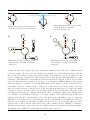
problem. Figure 3.5 gives an example of this problem, and shows 4 ways to resolve it.
Pairs can also be broken when var backbone range commands refer to one side of a base pair.
In this case, R2R will detect that this command was responsible for the problem (Figure 3.6). If
you have variable-length stems, you should use the var stem or var hairpin commands.
Key points:
• Pairs can be broken due to the consensus rules, and Figure 3.5 shows 4 ways to resolve the
problem.
• Pairs can also be broken due to variable-length backbones.
• R2R error messages often refer to lines or columns in the input Stockholm-format file. The
left-most column is numbered zero. The first line is numbered one.
3.5
The place explicit command
R2R encodes defaults for the layout of RNAs that work in many cases, but often you will want
to change this layout. The place explicit command allows you to position nucleotides relative
to one another using explicit relative or absolute coordinates (Figure 3.7). The syntax for the
command is:
place explicit label relative-label place-angle x-relative y-relative x-absolute y-absolute
next-angle
(illustrated with an example in Figure 3.7). The nucleotide at position label is positioned relative to
the nucleotide at position relative-label. The coordinate system of (x-relative,y-relative) is based on
the direction of the nucleotide at relative-label rotated by place-angle degrees. The x,y coordinates
(x-absolute,y-absolute) are added to this position. Both relative and absolute distances in the
19
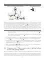
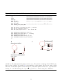
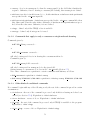
Figure 3.7 The place explicit command
B # STOCKHOLM 1.0
A
5
un
its
1
G
A
45°
90°
C
biologist
AACCCUUCGGAAACGGAGUAA
chemist
AACCCUUGCUUCGGCGAGUAA
physicist
AUCCCAUUUCUUGAAGAGAAA
#=GC SS_cons
<<...>><<....>>......
#=GC R2R_LABEL .......a.......b..c..
#=GF R2R place_explicit a a-- 0 1 0 0 0 0 f
#=GF R2R place_explicit b b-- +45 1 0 0 0 +90 f
#=GF R2R place_explicit c c-- -45 1 0 0 0 -90
//
demo-pe
C
5´
C
C
b--
A U
A
A
GAG
c--
R
a--
D mini-ykkC
CG
A
A
G C
G C
R Y
5´
start
CG
A
R
G C
G C
G C
7-39 nt
G
U
A
0-10 nt
SD
R
R
R
R
1-228 nt
(90th percentile: 33)
(A) Schematic of the positioning system in the place explicit command. The diagram illustrates the
effect of the command place explicit G A -45 5 -1 0 0 -90, which defines how the nucleotide labeled
G is positioned depending on the position of the nucleotide A. The direction of the backbone at the A (gray
array pointing right) is rotated -45 degrees to form the black arrow. The position proceeds 5 drawing units
along the black arrow, and -1 unit orthogonally to the black arrow. This is where the G is positioned. The
direction of the backbone of the G (gray arrow pointing up) is taken by adding -90 to the direction of the
backbone at the A. The two zeroes mean that no absolute positioning is used. One drawing unit is equal to
the distance between consecutive nucleotides along the backbone. (B) Hypothetical Stockholm alignment
to demonstrate place explicit command (contents of the file demo/demo-pe.sto). Note that the f at
the end of the first and second place explicit commands directs R2R to “flip” the backbone such that
the 30 side of a base pair is on the left of the 50 side, instead of the usual right side. The second flipping
command flips the orienation back to the default for the 30 tail of the hypothetical motif. Synthesizing an
appropriate joke based on the organisms from which the hypothetical RNA sequences were taken is left
as an exercise for the reader. (C) Annotated raw output of R2R when run on the alignment in part B.
Nucleotide positions that were the referent of place explicit command (i.e., a--, b-- and c--) have a
blue arrow indicating the direction of the backbone at that position. (D) Raw R2R output of the mini-ykkC
motif (demo/22/mini-ykkC.sto) [13], which uses a place explicit command to change the direction of
the var backbone range just before the SD sequence.
20
place explicit command are specified in drawing units, where 1 drawing unit is equal to the
standard internucleotide distance between consecutive nucleotides (by default 0.105 inches). The
direction of the nucleotide at label is the angle at relative-label rotated by next-angle degrees.
An optional f at the end of the command directs R2R to “flip” the stem (Figure 3.7B,C). Flipping
is analogous to applying a twist to the RNA. Where R2R normally positions the 30 nucleotide
of a base pair to the right of its partner, flipped regions will cause the 30 nucleotide to be on
the left. Flipping is used only sometimes, but Figure 3.7C shows a typical example where it is
useful to avoid crossing stems. A real-world example of this usage is the IMES-4 motif [14] (see
demo/exceptional/IMES-4.sto).
Section 5.8.2.6 explains the command in more detail.
More advanced usages of place explicit are necessary for the “in-line” layout of complex
pseudoknots (Section 3.8.3). I explain more about place explicit commands and their semantics
in that section. You can use set the showPlaceExplicit variable to true, in order to see the
place explicit commands in the context of the structure. This is demonstrated in the same
section (Section 3.8.3).
3.6
Multistem junctions and turning internal loops
Multistem junctions are a structural element within a RNA secondary structure in which a loop
includes more than two base pairs (e.g., see Figure 3.8). This section can be skipped if you are
drawing RNAs that don’t have multistem junctions. However, the material in this section is also
sometimes useful for turning the direction of the stem at internal loops (see Figure 3.14 for an
example of an internal loop).
There are three ways to draw multi-stem junctions with R2R:
• The junction is laid out perfectly on a circle, and stems are allowed to go in arbitrary directions.
This is the default. It usually looks acceptable (except when nucleotides clash), although I
think it’s typically not the most aesthetic solution.
• Manual layout using place explicit commands.
• Automated solutions that attempt to position the junction on a circle as well as possible,
but subject to constraints on the directions of the stems. This allows for orthogonal stems, a
design feature that I think tends to result in more attractive layouts.
3.6.1
Simple circular layout
The default circular layout for multistem junctions is demonstrated in Figure 3.8. This is the layout
that R2R uses if you do not give R2R any instructions on how to draw the multistem junction.
3.6.2
Manual layout of multistem junctions
Manual layout of multistem junctions can be accomplished by positioning the stems using place explicit commands, and directing the layout of the single-stranded regions using the bulge command. Since the use of these commands would result in many labels to identify the various positions,
R2R has the multistem junction bulgey command, for which only one label needs to be defined.
21
Figure 3.8 Simple circular layout of multistem junctions
A
B
multistem_junction_circular
M allstems-any-angle draw_circ
U R
CR YA
R
U
U
U
R
U R
CR YA
R
U
U
U
R
0-3 nt
5´
0-3 nt
M
Y R
G C
5´
C
D
multistem_junction_circular
M allstems-any-angle flipstem 1
stem 0
CR Y
R U RA
U
U
U
R
stem 1
0-3 nt
5´
Y R
G C
Y R
G C
Y CG
C
G
C GY
C
U G
C G
C G
G
G
C
C
U
CU
A
C
G
AC C
C G
G
CU
Y
C A
GR G C C C
Y
CG
A
G
Y
G
C
Y R AC
G
YR
R
G
G
G Y
YA
U
C
G
G
G
Y
A
Y
AC G
G
A
U A
A
G C
CGG
G C
5´
GGY Y
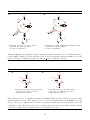
(A) Default layout of a hypothetical three-stem junction that is modeled on a multistem junction in HEARO
RNA [14]. This output is based on the files demo/demo-multistem.sto and demo/demo-multistem.r2r meta. (B) In the default layout, nucleotides along the multistem junction are positioned on a circle. The
R2R command shown here directs R2R to draw this circle. The command refers to position “M”. Position
M is labeled, and is the left nucleotide of the base pair that encloses the whole multistem junction. (Note:
the command should be one line, but is displayed on multiple lines in this figure so it fits the page.) (C)
Stems can be flipped so that they are directed into the multistem junction. This can save space when the
multistem loop is larger than one of the stems. The stems are numbered starting at zero. The enclosing
stem does not have a number, and cannot be flipped. (D) The SAM-IV riboswitch [15] is drawn using
the default layout of its multistem junction. (Note: the gray lines correspond to pseudoknots. Drawing of
pseudoknots are explained in a later section of this tutorial.)
22
Figure 3.9 Manual layout of multistem junctions
A
YC
B multistem_junction_bulgey 1
G
C
C G
C GY
U
C G
C G
AC G
U
AC G
Y
Y
G C C
C
G
G
G G C U G C U G R Y CG C
R
G
C
G Y
U
C
G
A
C
G
A
C
Y
R
G
C
G
CC
YA
A
R
G
A
G
Y
Y
YAC G
G
A
U A
A
G C
CGG
G C
5´
GGY Y
J0 -45 1 0 -3 -2 -90
J1 -45 1 0 0 0 -90
C G
G C C
G C C GG
R Y CJ1
G
U
YRG
J0
G
YA
A
G
YAC G
U A
G C
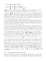
(A) The published layout of SAM-IV riboswitches [15]. Layout of the multistem junction uses the
multistem junction bulgey command. This drawing is based on the file demo/SAM-IV/SAM-IV.sto,
in multistem=original mode. This mode is entered in the .r2r meta file using the specification define
multistem original. (Note: at the time at which SAM-IV riboswitches were drawn, manual layout was
the only option for drawing multistem junctions. Also, the gray lines are for pseudoknots, as described
in Section 3.8.2.) (B) R2R command to draw the multistem junction, and larger view of the multistem
junction. The junctions called “J0” and “J1” are labeled. There are no nucleotides within junction J1.
In the multistem junction bulgey command, the stems within the multistem junction are
positioned using functionality similar to place explicit commands. The junctions are then positioned automatically between the stems by positioning them on circles (equivalent to the bulge
command). Figure 3.9 shows an example.
Junctions are identified using the symbols J0, J1, J2, etc. Junction J0 identifies the junction
between the enclosing stem and the next 50 -most stem. Junction J1 identifies the junction between
this next 50 -most stem, and the next stem to that (i.e., the immediately 30 stem). Positioning of
J0 is equivalent to a place explicit command that positions X relative to Y, where X is the left
nucleotide of the stem on the 30 side of the junction J0 and Y is the left base-paired nucleotide of
the stem on the 50 side of the junction J0. For junctions J1, J2, etc., Y is the right nucleotide of
the stem on the 50 side of the junction. An equivalent viewpoint is that X and Y are the basepaired nucleotides immediately 30 (X) and 50 (Y) to the nucleotides within the junction. This is
also illustrated in Figure 3.9.
The multistem junction bulgey command also provides alternate layouts for the bulges, such
as flipping the direction of the bulge, and some linear layouts for the junctions. It is also possible to
position the 50 base-paired nucleotides in all stems relative to the enclosing stem, rather than to the
previous stem by using J1/base in place of J1. These variations are described in Section 5.8.3.1.
3.6.3
Automated multistem junction layout with direction constraints
R2R provides the ability to automatically determine a layout of a multistem junction, given userspecified directions in which each stem must go. This functionality requires that CFSQP is available
(see Chapter 2).
This automated layout facility is refered to as the solver commands in this manual, and is
applied with one of the following three related commands:
23
Figure 3.10 Automated layout of multistem junctions
A U R
zero degrees
B
R Y
A
C
R
U
negative angles
U
U
R
0-3 nt
5´
s1
Y R
G C
C
R
U
R
R YA
R
U
U
0-3 nt
R
5´
0-3 nt
multistem_junction_circular_solver
M s0 0 m s1 -90 m s2 0 m draw_circ
D
positive angles
s2U
U R
CR YA
U
R
U
U
C
Y
s0 G
5´
C
C
U
C
C
AC
AC
G
G
GCUGRYC
G GC U
C
C
C C G A C G A C Y RYG
A
R
A
Y
G
Y
AC
U
G
G
5´
G
A
C
C
multistem_junction_circular_solver
M s0 0 ai=0 s1 -90 ai=0
s2 0 ai=0 draw_circ
R
C
YC
YC
G
C
G
GY
G
G
G
U
G
C
CCC
Y R
G C
E
G
G
G
U
G
A
Y
Y
R
G Y
C
G
Y
G
A
A
CGG
GGY Y
C
C
CG
U
G
C
C
C
C
C
CG U
A
G
AC
A
AC
C CU
Y
R G
A GR G
C
Y YCG
R
YG
A
G
Y
A
C
U
G
G
5´
G
C
G
GY
G
G
G
U
G
C
CC
G
A
C
C
Y
Y
C
G
R
G
G Y
G
C
U
G
G
A GY
A
A
CGG
GGY Y
multistem_junction_circular_solver 1
s0 0 ai=0 s1 -45 ai=0 s2 0 ai=0
draw_circ
multistem_junction_circular_solver 1
s0 0 ai=0 s1 -90 ai=0 s2 0 ai=0
draw_circ
(A) Layout of the demo structure used in previous figures, using the solver. The solver command is given
below the drawing. The lower case “m” parameters say that the circle should intersect in the midpoint
(m) of stems. Note that the length of the variable-length region (marked as “0-3 nt”) is adjusted by the
solver to optimize the circular layout. (The drawing is based on the file demo/demo-multistem.sto, with
solver1=1.) (B) Illustration of stem numbers and directions from the diagram of part A. The enclosing
stem is s0, then the stems are number s1, s2 from 50 to 30 around the multistem junction. The stem s0
defines the angle zero, as indicated. As usual within R2R, positive angles are in the clockwise direction,
and negative angles are counter-clockwise. Thus, s1 is oriented in the direction -90 (going to the left),
while s2 is in the direction 0 (up the page). If the enclosing stem (stem s0) were rotated, the angles
of stems s1 and s2 would also rotate to be the same, relative to the enclosing stem. The angle of the
enclosing stem (stem s0) can be changed, which has the effect of rotating the entire picture. This is purely
for convenience, and is illustrated in Figure 3.11. (C) A variation on the drawing in part A. The ai=0
parameters directs R2R to automatically decide on the intersection point with the circle for each stem.
This leads to a circle that better goes through each nucleotide. (D) Drawing of the SAM-IV riboswitch [15]
using the solver. In this case, the bulged Y within stem s1 is very close to the A in the junction between
stems s0 and s1. The positions of these nucleotides could be adjusted in Adobe Illustrator of Inkscape.
Alternately, the stem s1 could be rotated to avoid this problem, as demonstrated in the next sub-figure.
(E) Drawing of the SAM-IV riboswitch with an alternate angle for stem s1.
24
Figure 3.11 Automated layout of multistem junctions: unusual stem directions
AA
A
B
G A
A
U
A
AU
A A
G R
Y
UG
CA
U RYU
C
A
A
U
A
A
A
R
UY
U
G
R
UR Y
Y G
C
U
G C
U A
AA
Y R
A
A
A
U
U
A
G
U
G
U C
A
U
G
U
A R Y UC A
C
U Y R AAU
U
R
Y G
C
U
AA
5´
multistem_junction_bulgecircley_solver
j s0 -15 ai s1 -135 ai s2 -45 ai
s3 45 ai s4 105 ai
C
D
A
A
U
U
A
AA
G A
Y R
U
A
G
U
G
U C
A
A
A
G
U
A R Y UC A
C
U Y R AAU
U
U
U
A
AA
G A
Y R
U
A
G
U
G
U C
A
R
Y G
C
U
AA
zero degrees
G
U
A R Y UC A
C
U Y R AAU
U
R
Y G
C
nucleotide referenced
by align:Y
nucleotide referenced
by align:X
U
AA
multistem_junction_bulgecircley_solver
j s0 -15 ai s1 -135 ai s2 -45 ai s3 45 ai
s4 105 ai align_nuc_centers_angle 60 align:X .
align:Y . align_angle -30 0 4
This figure illustrates the strategy of using the default circular layout to suggest aesthetic stem directions. In this case, I was not able to find directions that are multiples of 90 or even 45 that worked
well. This example is based on a multistem junction in the manA motif [16] (see demo/104/manA.sto
for the full motif). (A) Default circular layout of this motif. (This drawing is derived from the file
demo/demo-multistem-manA.sto.) (B) Layout using solver, with stem directions that roughly match the
default orientations in part A. Stem s0 is rotated 30 degrees clockwise in this figure. The directions of
stems s0 and s4 are symmetric about the vertical axis, which results in an aesthetic design. (Note: R2R
does not draw the 50 marking since the 50 nucleotide’s direction is not orthogonal to the X or Y axis.) (C)
Alignment constraints are added to the layout of part B. align angle -30 0 4 dictates that the stems
s0 and s4 should be vertically aligned. (The alignment angle -30 is used because the enclosing stem is
rotated by 30 degrees; see part D.) The constraint align nuc centers angle 60 align:X . align:Y .
forces the midpoint of the nucleotides defined by align:X to be horizontally aligned with the midpoint of
the align:Y nucleotides. This alignment further improves the symmetry. Note that R2R cannot aesthetically satisfy any arbitrary constraint, and so stems s1 and s3 cannot be vertically aligned in this layout.
(D) The drawing of part C is annotated. The nucleotides that were aligned are drawn in alternate colors
as shown. The align:X nucleotides were vertically aligned with each other when their stems (s0 and s4)
were aligned. Zero degrees is defined as the direction of stem s0 (as shown), so the vertical direction is
-30 degrees. The solver directives draw circ and draw zero degrees were added to draw the multistem
junction circle, and the zero degrees mark, and nuc color was used to color the align:X and align:Y
nucleotides.
25
Figure 3.12 Automated layout of multistem junctions: additional example
CAA
CAA
A
B
0-2 nt
A
A
A
G
Y
C
A
Y R
Y R
Y RC
GC
C
A
G
A
G
R
R YC
A
G UY
5´ G GC
A
A
C
C
A
G
RR
YY
RGA
C A C GG
C G
A
A
C
C
A
Y R
Y R
Y RCC
A
0-2 ntG C
C
C
A
A
A G
A
A
A
RR
G
G
Y
YY
A
A
RGA
G
A
R C
G
R Y
G
A
CA C GGA
G UY
C G
5´ G GC
C G
U A
G A
A
2 nt
A
C
A
C UG
A
C G
U A
G A
A
A
G
G
2 nt
A
C UG
multistem_junction_circular_solver
j s0 0 m s1 -45 m s2 +45 m
s3 +135 m flipstem 2
multistem_junction_bulgecircleynormals_solver
j s0 0 m s1 -45 m s2 +45 m
s3 +135 m flipstem 2
This figure illustrates an additional example of a multistem junction drawing, based on a multistem junction
found in IMES-1 RNAs [14]. (The drawing is based on the file demo/demo-multistem-IMES-1.sto.) (A)
Layout of the given command. (B) Layout a different solver command, as shown.
Figure 3.13 Automated layout of multistem junctions: starting point is important
A
A
U
G
G
U
C
A
G
U
UUC
C
C
AAG
GC C
4 nt A
G
A
U
5´
A
A
C
C
A
CG
U
U
G
C
U
A
B
A
U
G
G
U
C
A
G
U
UUC
C
C
AAG
GC C
4 nt A
G
A
U
5´
5 nt
multistem_junction_circular_solver
J s0 0 ai s1 -90 ai s2 0 ai
align_stem_horiz 0 2
A
A
C
C
A
CG
U
U
G
C
U
A
5 nt
multistem_junction_circular_solver
J s0 0 ai s1 -90 ai=0 s2 0 ai=1
align_stem_horiz 0 2
This drawing is based on a multistem junction in HEARO RNA [14] that is different from the earlier
multistem junction shown. (The drawing is based on the file demo/demo-multistem-HEARO2.sto.) (A)
Layout of the given command, with ai parameters using the default midpoint as the initial point for the
optimization search. (B) Layout of the given command, with ai=0 and ai=1 specifying alternate starting
points. The resulting layout is slightly different, and I think a bit better.
26
• multistem junction circular solver
• multistem junction bulgecircley solver
• multistem junction bulgecircleynormals solver
All solver variants use a very similar syntax and framework. They are explained in full detail in
Section 5.8.3.2, but for now we will see the most essential aspects of the commands.
Examples of the solver commands are given in Figures 3.10, 3.11, 3.12 and 3.13. The command
begins with a solver command, then specifies a label. As with previous multistem junction
commands, the label denotes the left nucleotide in the base pair that encloses the multistem junction.
Then, then properties of each stem in the multistem junction are written. The enclosing stem is
named s0, then each stem from 50 to 30 are labeled s1, s2, ... (see Figure 3.10). The names for the
stems are different from those of multistem junction commands described earlier in this tutorial. In
particular, the enclosing stem can be explicitly referenced (as s0).
For each stem, the desired angle of that stem is given, in a coordinate system defined by the
enclosing stem (Figure 3.10B). The point at which the circle should intersect the inner base pair of
each stem is also specified. Useful values are m (intersects the midpoint of the base pair), l (intersects
the center of the left nucleotide in the base pair), r (intersects the right nucleotide in the base
pair) and ai (automatically solve the intersection).
To find a good layout of a particular multistem junction, it is often necessary to play with several
formulations, involving different stem angles and solvers. One strategy to finding good directions
for the stems is to use the default circular positioning of the multistem junction to find directions
that fit the circle perfectly, then consider nearby angles that are multiples of 90 degrees, or have
other pleasing characteristics. See Figure 3.11 for an example. As noted above, the starting point
for the circle-intersection point of each base pair can sometimes have an effect on the solution.
Variable-length backbones (introduced using the var backbone range command) can help to
improve aesthetics of drawings, as the solver is permitted to change the length of the lines to improve
the circularity of the layout. This additional degree of freedom can be helpful. Of course, some
multistem junctions do not have variable-length regions, so this tactic cannot always be used.
Additional examples illustrating aspect of the solver commands are shown in Figures 3.12 and
3.13.
Note: the starting point for the intersection can be supplied for automatic inference, and this
sometimes assists the solution, as the problem that the computer has to solve is highly non-linear,
and the computer can easily get stuck in local minima. See Section 5.8.3.2 for details on various
initial values that can be set. For example, ai=0 means start with the intersection at the left
nucleotide and ai=1 means start at the right nucleotide of the base pair. Any number from 0 to
1 can be given, so ai=0.5 means start at the midpoint. The circle intersection parameter is only
relevant to multistem junction circular solver; the multistem junction bulgecircley...
commands try to have both nucleotides on the circle. However, other parameters are relevant to
the bulgecircley variant commands. You can also add try harder to the multistem junction circular solver command to improve it’s ability to find a good global optimum (details in Section 5.8.3.2).
3.6.3.1
Solving multistem junctions can be slow
On even modern machines, the computer can take a significant amount of time to solve the problem.
Often the solver goes through a period of very gradually improving the solution, and many iterations
are required to reach an optimal solution—and the difference in the ultimate solution is noticeable.
27
Figure 3.14 An internal loop with a 90-degree turn
A
B
turn_stem_at_internal K +1 r
left
C
YC
C
C
U
C
C
CC
C
G
AC
C
G
AC
G C
G
A U
G
A
GCUGRYC
Y
RCGACYRG
YA
G
right
G C
A U
A
GC
Y
RCG
K
multistem_junction_circular_solver
K-- s0 0 ai s1 90 ai
CC
C
G
C
G
G C
A U GCUGRYC
A
Y RC G A C Y R G
Y
D
CC
multistem_junction
_bulgecircleynormals_solver
K-- s0 0 ai s1 90 ai
C
G
C
G
G C
A U
A
GCUGRYC
Y
RCGACYRG
Y
E
G
C
G
GY
G
G
G
U
G
C C
CC G
YAC
U
G
G
5´
Y
Y
G
R
G
G Y
U
C
G
G
A
Y
G
G
A
A
A
C
CGG
C
GGY Y
multistem_junction
_bulgecircleynormals
_solver
K-- s0 0 ai s1 45 ai
CG
G
C
C
C
CG U GCUGR Y C
A
A
CGACYRG
Y R
Y
This drawing is based on SAM-IV riboswitches [15, 13], in the file demo/22/SAM-IV.sto. (A) An R2R
command to turn an internal loop in SAM-IV riboswitches. The label K refers to the 50 -most nucleotide
within the 50 part of the internal loop, as shown. (You can also use the 30 -most part of the 30 part of
the internal loop.) The stem can be turned 90 degrees clockwise or counter-clockwise. The value +1 (as
shown) is clockwise, while -1 would be counter-clockwise. R2R will decide the layout on one side of the
internal loop. The value r will make R2R use the right side (i.e. 30 side) for positioning, while l is for
the left side. (B) The turned internal loop in the context of the full SAM-IV consensus. (C-E) Turning
the internal loop using solver commands. Since the solver commands require the label to be the left
nucleotide of the enclosing base pair of the internal loop, we use the label K--.
Therefore, I have conservatively set the solver to use up to 100,000 iterations. You can decrease
this number with an R2R command like SetDrawingParam solverMaxIters 50000.
I have also implemented a “caching” strategy, in which solutions to problems solved by CFSQP
are store in a file that is associated with the .r2r meta input file. These files end in the extention
.solver-cache. If you re-run R2R, but do not change anything related to the multistem junction,
the solution will be re-used. By deleting the .solver-cache file, you can force a re-computation.
Note: R2R is designed to detect subtle changes that can change the problem, and R2R will recompute the solution in these cases. For example, if you change the value of internucleotideLen
using the SetDrawingParam command, this changes a parameter in the multistem junction NonLinear Program, even though it is an indirect effect.
3.6.4
Internal loops
Internal loops and bulges are unpaired regions that interrupt stems. It is often desirable to turn
the direction of the stem at these loops for two main reasons. First, bulges and highly asymmetric
internal loops can have a distorted look due to having too many nucleotides on one side. A turn
can give more space to the longer side, improving the clarity and aesthetic quality of the drawing.
28
Second, turning of stems can resolve problems with other regions of the structure that might overlap,
use space inefficiently, or otherwise be undesirable.
R2R has a special command for turning the direction of the stem at internal loops or bulges.
This command restricts turning to +90 or -90 degrees, however. The command, turn stem at internal, is demonstrated in Figure 3.14, and documented in detail in Section 5.8.2.5.
The turn stem at internal command is limited both in the angles it can handle, and in the
layout policy. You can use the solver commands that are designed for multistem junctions on
internal loops or bulges. An internal loop is simply a multistem junction with only 2 stems, for the
purposes of these commands. The application of solver commands to internal loops is demonstrated in Figure 3.14.
Note that R2R does not distinguish between internal loops and bulges, as RNA biologists often
do. For R2R, a bulge is simply an internal loop with zero nucleotides on one side.
3.7
Modular structures
I define modular structures as sub-structures of an RNA that are sometimes, but not always,
present in a conserved RNA structure. Many RNAs, for example, have stems that are sometimes
present. To draw a consensus, it is often desirable to reflect these modular structures, and their
relative frequencies. As with other frequencies, R2R weights sequences using the GSC algorithm,
and calculates the weighted frequency of the set of sequences that do have the modular structure.
(See Chapter 4 for details.)
Figure 3.15 demonstrates the drawing of two modular substructures in the context of a simple,
hypothetical motif. It covers hairpins that are sometimes, but not always, present. It also covers a
loop that has distinct structures that are possible, namely the stable GNRA or UNCG tetraloops.
The figure legend gives the commands that would be run to process files with modular structures.
The basic idea for processing modular structures in R2R is (1) to define a predicate that determines which sequences exhibit a given substructure (e.g., which sequences have the optional
hairpin), (2) extract those sequences into a new .sto file using a Perl script that is part of R2R and
(3) draw the new file. Predicates can be defined using either regular expressions or using Boolean
operations using a subset of the Perl programming language.
Regular expressions are a mathematical formalism for describing sequence patterns [1]. Some
examples are given in Figure 3.15. To implement these regular expressions, I used Perl, and consequently R2R uses the Perl syntax to specify regular expressions. To learn about all the capabilities
of regular expressions in Perl, one good Web site is http://www.perl.com/doc/manual/html/pod/
perlre.html.
Regular expression predicates operate on subsequences in columns defined by lines of the form
#=GC SUBFAM LABEL .... For example, #=GC SUBFAM LABEL TERM would define columns that can
now be referred to as “TERM”.
Here are some examples of regular expressions that illustrate features relevant to RNA. For four
columns with no gaps, G[A-Z][AG]A defines the GNRA tetraloop. The text in square brackets ([
and ]) define a set of symbols. [A-Z] is the set of upper-case letters, while [AG] defines the symbols
A or G. A period (“.”) is a special symbol that stands for any character, so in order to look for a
gap character you should enter [-.].
A few other special symbols are often relevant. The caret symbol “^” (shift-6 on a standard US
keyboard) stands for the beginning of a subsequence, while the dollar sign “$” represents the end of
a subsequence. The asterisk “*” represents zero or more occurrences of the previous symbol. Thus,
the expression ^[-.]*$ matches all subsequences that consists only of gap characters.
29
Figure 3.15 Modular structures
A
B
# STOCKHOLM 1.0
one
two
three
four
#=GC SS_cons
#=GC R2R_LABEL
#=GC SUBFAM_LABEL_TERM
#=GC SUBFAM_LABEL_OPT
#=GC SUBFAM_GNRA_R2R_LABEL
#=GC SUBFAM_UNCG_R2R_LABEL
#=GC SUBFAM_OPT_R2R_LABEL
GAGAAA.UCAACCCUUGGGGGAGCA
AGUUCG.CUAAUCCUAGGAGGAGCA
GGGAAACCCAA........GGAGCA
AGCAAC.CUAA........GGAGCA
<<.....>>..<<....>>......
.........................
..xxxxx..................
.............x...........
-.......-----------------.......---------------------------........------
demo-modular
5´
G C
R Y
demo-modular-GNRA
subfam_weight=0.230158
23%
AA
GGAGC A
AA
G A
A U
demo-modular-OPT
demo-modular-UNCG
subfam_weight=0.5
subfam_weight=0.269842
50%
27%
U
C G
C G
Y R
UC
U G
G C
#=GF
#=GF
#=GF
#=GF
#=GF
#=GF
SUBFAM_REGEX_PRED HAS_GNRA TERM G[A-Z][AG]A
SUBFAM_REGEX_PRED HAS_UNCG TERM U[A-Z]CG
SUBFAM_REGEX_PRED FOUR TERM ^[.]*[A-Z][A-Z][A-Z][A-Z][.]*$
SUBFAM_PERL_PRED GNRA return $predValue{HAS_GNRA} && $predValue{FOUR};
SUBFAM_PERL_PRED UNCG return $predValue{HAS_UNCG} && $predValue{FOUR};
SUBFAM_REGEX_PRED OPT OPT [A-Z]
#=GF
#=GF
#=GF
#=GF
#=GF
#=GF
//
SUBFAM_GNRA_R2R no5
SUBFAM_GNRA_R2R set_dir pos0 -90
SUBFAM_UNCG_R2R no5
SUBFAM_UNCG_R2R set_dir pos0 -90
SUBFAM_OPT_R2R no5
SUBFAM_OPT_R2R set_dir pos0 -90
C
23%
5´
G C
R Y
AA
G A
A U
27%
UC
U G
G C
A A GGAGC A
50%
U
C G
C G
Y R
(A) The Stockholm alignment and R2R drawing commands for a hypothetical modular structure.
This is the file demo/demo-modular.sto. (B) Raw output of R2R. To extract the Stockholm file for
the predicate GNRA, for example, the command perl ../src/SelectSubFamilyFromStockholm.pl
intermediate/demo-modular.cons.sto GNRA > intermediate/demo-modular-GNRA.sto
was
used, followed by inference of the consensus using ../src/r2r --GSC-weighted-consensus
intermediate/demo-modular-GNRA.sto intermediate/demo-modular-GNRA.cons.sto 3 0.97 0.9
0.75 4 0.97 0.9 0.75 0.5 0.1. The file intermediate/demo-modular-GNRA.cons.sto was included
in demo-modular.r2r meta. Similar commands were run for the UNCG and OPT predicates. (C) Integration
of the modular structures into a consensus diagram. This drawing was created in Adobe Illustrator using
the output of R2R shown in part B.
30
R2R also provides Boolean operations that can combine the values of other predicates. These
predicates also exploit Perl, and therefore inherit a Perl-like syntax. In these predicates, the expression $predValue{GNRA}, for example, would evaluate to true if the predicate named GNRA is true
for a given sequence. Two ampersands (&&) represents the Boolean “and” operation, which evaluates to true if the two sub-expressions are true. So, $predValue{GNRA} && $predValue{FOUR}
is true if the predicates GNRA and FOUR are both true. Similarly, two pipe symbols (||) denote the
Boolean “or” operation, which evaluates to the true if either of the sub-expressions are true. The
exclamation mark ! is the Boolean not operation, so the expression !$predValue{GNRA} represents
all sequences that do not match the GNRA predicate. Warning: if you use Boolean predicates, you
must define predicates they use within $predValue earlier in the .sto file, since R2R will evaluate
predicates in the order in which they appear in the .sto file.
The script SelectSubFamilyFromStockholm.pl evaluates predicates and creates a new .sto
file with the subset of sequences. It also modifies which commands are present in the file, in order
to use commands that are appropriate to drawing the modular structure. All lines beginning with
#=GF R2R or #=GC R2R are by default removed. At the same time, for example with the
predicate GNRA, lines beginning #=GF SUBFAM GNRA R2R are changed to #=GF R2R so that
they now become processed. Similarly, lines beginning #=GC SUBFAM GNRA R2R... are changed to
#=GC R2R....
Chapter 6 gives further details on the commands.
3.8
Pseudoknots
Pseudoknotted RNAs typically lead to confusing drawings when drawn with the default layout of
R2R. Therefore, to help you to plan the final layout better, the first thing to do with an RNA
structure that has a pseudoknot is usually to make R2R ignore the pseudoknot, which can be
accomplished with the ignore ss except for pairs command. I give an example of this command
in the next section, since it leads naturally to a “callout” style of pseudoknot drawing.
3.8.1
A note on the representation of pseudoknotted secondary structures within Stockholm files
R2R uses a non-standard method for writing consensus secondary structures for motifs with pseudoknots. To describe pseudoknots, in addition to the standard #=GC SS cons line, there can be
other lines of the form #=GC SS consX for any string X (typically, I call them #=GC SS cons 1,
#=GC SS cons 2, ...). In the pseudoknot examples in this section, you will see #=GC SS cons 1
used. GOLLD RNA [14] has 5 pseudoknots (see demo/exceptional/GOLLD.sto), and uses up to
#=GC SS cons 5. When you use extra #=GC SS cons ... lines, I recommend that they each only
contain only one stem (possibly with bulges/internal loops), and not more complex structures. R2R
is best tested with this convention.
I find this representation of pseudoknots within Stockholm files to be convenient, because all
#=GC SS cons lines are interpreted in the same way.
3.8.2
Pseudoknots drawn with callouts
Figure 3.16 gives an example of an RNA with a pseudoknot that is drawn using a callout style. This
style depicts the pseudoknot pairing in a “callout” (Figure 3.16C) that also allows R2R to shade
covarying base pairs. To achieve this, we consider the pseudoknot as a modular structure, and make
31
Figure 3.16 A pseudoknotted RNA drawn in callout style
A # STOCKHOLM 1.0
rope
speed
topology
#=GC SS_cons
#=GC SS_cons_1
#=GC R2R_LABEL
#=GC SUBFAM_pknot_R2R_LABEL
AGGCAUUUGAACCAUAUUGUGCGCCUAACAUC..GCCAAAGCACAA
GGGUAUUUGAACUGUAUUAUGCACCCAGCAUAAUGUGGAACCAUAA
AGGUAUUUGAACCGUAUUGUGCACCUAGCAUGA.GUUAAAGCACAA
<<<<..................>>>>....................
..................<<<<..................>>>>..
...............................1.2...3........
------------------....------------------....--
#=GF R2R ignore_ss_except_for_pairs _1 outline
#=GF R2R var_backbone_range 1 2
#=GF R2R place_explicit 3 3-- -45 1 0 0 0 -90
#=GF
#=GF
#=GF
#=GF
#=GF
//
SUBFAM_PERL_PRED
SUBFAM_pknot_R2R
SUBFAM_pknot_R2R
SUBFAM_pknot_R2R
SUBFAM_pknot_R2R
pknot return 1;
subst_ss _1 primary
no5
outline_nuc all
set_dir pos0 90 f
B
demo-pknot-callout
CY
A
A
G
U
U
U
AY
G
G
R
5´
C
RU
A
U
U
R
U
G
RC
C
C
Y
ARCAU
A
A
Y
A
C
1-3 nt
GY
CY
A
A
G
U
U
U
AY
G
G
R
5´
RU
The demo motif
A
U
U pseudoknot
R Y
R
U A
U
G
G C
C
C
R
C
C
Y
1-3 nt
ARCAU
GY
A
A
Y
A
C
A
A
R
A
A
R
demo-pknot-callout-pknot
subfam_weight=1
R Y
U A
G C
C
(A) The Stockholm file demo/demo-pknot-callout.sto. The structure of this hypothetical RNA is inspired by that of SAM-V riboswitches [8], but is simplified for this example. (B) The raw output of R2R
when run on demo/demo-pknot-callout.r2r meta / demo/demo-pknot-callout.sto. (C) Assembled
drawing. To create this drawing, the components of part B were combined using Adobe Illustrator.
32
R2R draw it separately. Modular structures were explained in Section 3.7. Their application to
pseudoknots is somewhat simpler, since all sequences presumably have the pseudoknot, so there is
no need to define any regular expressions.
The line #=GF SUBFAM PERL PRED pknot return 1; (e.g., see Figure 3.16A) defines the pknot
“modular” structure as applying to all sequences. R2R commands and #=GC lines beginning with
SUBFAM pknot then define commands that should be run to generate the pknot structure. The
actual drawing is initiated by a line in the .r2r meta file, and running extra commands to create
the pseudoknot view of the RNA structure, as in Section 3.7.
It is also possible to draw callout-style pseudoknotted structures without the use of the modular
structure logic, but instead using the define and ifdef commands to draw the main RNA and
separately draw the pseudoknot. The associated files demo/demo-pknot-callout-ifdef.sto and
demo/demo-pknot-callout-ifdef.r2r meta demonstrate how to do this.
Once R2R has drawn the pseudoknot and the main structure, these need to be assembled in
a drawing program like Adobe Illustrator or Inkscape. One style of this assembly is shown in
Figure 3.16C.
Note: R2R will attempt to automatically join the lines or arcs that comprise an outline corresponding to a pseudoknot. However, sometimes its heuristics will fail, and it might be missing some
lines, i.e., some nucleotides will not be outlined. In this case, try disabling the automatic joining
behavior:
#=GF SetDrawingParam outlineAutoJoin false
This case arises with the first pseudoknot in SAM-IV riboswitches [15], for which I disabled automatic joining (see demo/SAM-IV/SAM-IV.sto)
3.8.3
Pseudoknots drawn with in-line style
Sometimes the geometry of a particular RNA motif allows the pseudoknot base pairs to be drawn
without the use of a callout. In these cases, it is often desirable to use an “in-line” drawing of
the pseudoknots, as shown in Figure 3.17. However, even if you want to draw an in-line style, I
recommend starting with a basic callout-style drawing, because it’s easier to understand the RNA
and decide on a final layout.
Internal loops, bulges, terminal loops and multistem junctions are by default drawn along a circle.
However, adding place explicit commands that refer to positions within these loop regions will
cause them to be drawn in a straight line. In cases where you want a part of the original loop to
be drawn along a circle, you can use the bulge or bulge flip commands.
In order to achieve an in-line pseudoknot layout, it is often necessary to flip stems, using the f
option to the place explicit command. Sometimes it can be confusing to get the proper stems
flipped. It is useful to note that R2R has default rules for layout. When you use a place explicit
command, your command will override default rules. (Specifically it will override any conflicting
default rules.) To diagnose problems with flipped stems, try using the mark flip R2R command,
which shows you in the drawing whether each element is flipped or not. Another strategy is to simply
remove the f marking from place explicit commands that you might think should be flipped, and
see if that helps. Finally, you can use the command SetDrawingCommand showPlaceExplicit true
to show you how your place explicit commands were used in the positioning, and where default
rules were used (which you might want to override with additional place explicit commands).
The showPlaceExplicit option is demonstrated in Figure 3.17.
Examples of R2R-based RNA drawings with in-line pseudoknots are as follows. Most of these
use flipped stems.
33
Figure 3.17 A pseudoknotted RNA drawn in inline style
A A AY RU U A U R Y C A A G U U U AY R
A U
C G
C
B
# STOCKHOLM 1.0
rope
speed
topology
#=GC SS_cons
#=GC SS_cons_1
#=GC R2R_LABEL
#=GF
#=GF
#=GF
#=GF
#=GF
//
C
5´
R2R
R2R
R2R
R2R
R2R
G C
G C
R Y
ARCAU
GY
RAA
AGGCAUUUGAACCAUAUUGUGCGCCUAACAUC..GCCAAAGCACAA
GGGUAUUUGAACUGUAUUAUGCACCCAGCAUAAUGUGGAACCAUAA
AGGUAUUUGAACCGUAUUGUGCACCUAGCAUGA.GUUAAAGCACAA
<<<<..................>>>>....................
..................<<<<..................>>>>..
....a.................t...b....1.2..........3.
place_explicit t-- t 0 -1 0 0 0 0 f
place_explicit 3 3-- +45 1 0 0 0 +90 f
var_backbone_range 1 2
bulge a
bulge_flip b
demo-pknot-inline
RU AU
Y
U
AA
C
R Y
A
U
A
A
G C
G
A AR
C
U
UU A Y R
Y
G C
G
G C
R Y
5´
A
R C A U 1-3 nt
D
E
RU AU
Y
U
AA
C
R Y
A
U
A
A
G C
G
A AR
C
U
UU A Y R
Y
G C
G
G C
R Y
5´
A
R C A U 1-3 nt
def
11
def
def
10
1st
U
A
R Y
U A
def
11
def
The same RNA structure depicted in Figure 3.16 is now drawn with an in-line-style pseudoknot. (A)
R2R’s default drawing of the structure. R2R does not attempt to make a feasible in-line-style drawing
of a pseudoknot structure, since this is quite difficult, and sometimes not possible within R2R’s quality
constraints. (B) Stockholm input file. This is the contents of demo/demo-pknot-inline.sto. (Some
commands were removed, but these lines are not necessary to generate the drawing in part C.) (C)
Raw output of R2R when run on the Stockholm file in part B. (D) Output of R2R when run using
the command R2R SetDrawingCommand showPlaceExplicit true, which marks where place explicit
commands were used. The boxed region is shown at a larger scale in the next subfigure. (E) Expansion
of the region boxed in part D. The pink arrow labeled ‘11’ on the top left corner refers to a place explicit command on line 11 of the input .sto file (demo/demo-pknot-inline.sto). The pink line has
two arrowheads. The thicker one (pointing up and right) indicates the direction in which layout actually
proceeded, although it is not usually necessary to know this. The gray arrow on the left labeled ‘def’ shows
a default rule that R2R used to position these nucleotides. In this case, the default rule says that a helix
should be positioned in a linear arrangement. These arrows are sometimes useful to diagnose problems
with place explicit commands. The arrows and their labels are intentionally small so that they clearly
indicate the relevant nucleotides in an automated drawing. Most PDF and SVG viewers allow zooming in,
to expand the scale of these features.
34
• SAH [12, 13] (see demo/SAH/SAH.sto)
• PreQ1 -II [13] (see demo/22/preQ1-II.sto)
• The pfl motif [16] (see demo/104/pfl.sto)
• The ykkC-III motif [16] (see demo/104/ykkC-III.sto)
• The Downstream-peptide motif [16] (see demo/104/Downstream-peptide.sto)
.
3.9
Preparing presentations using projectors
This section concerns the default colors for shading base pairs, which indicate covarying mutations.
These colors were selected with journal papers in mind. The colors are clear in print or on a computer
monitor, yet are not too distracting. However, these colors are too light for many projectors.
Therefore, if you’re doing a talk and want the audience to be able to see the shading, I recommend
darker colors.
To modify the colors in an R2R drawing, you can add the following R2R command:
SetDrawingParam pairShadingColors rgb:156,199,153 rgb:152,199,222 rgb:235,138,126
(thanks to Kirsten F. Block for these RGB color values).
Or you can change the colors of an existing drawing program in a drawing program. Adobe
Illustrator allows you to select all object that have the same fill color as a selected object. So, you
can select one covarying (pale green) base pair, and then get all the others, to change this color.
3.10
How to draw GOLLD RNA from R2R output
As stated previously the published drawing of GOLLD RNA [14] was based on the most commonly
observed structural elements. Creating the drawing based on the output of R2R therefore requires
some assembly. The drawing is generated from the demo files demo/exceptional/GOLLD.sto and
demo/exceptional/GOLLD.r2r meta, and this description refers to the PDF or SVG output generated when R2R is run on those files. Most elements of the drawing come from the default drawing,
called “GOLLD”. However, the second multistem junction (numbered from the 50 end) is taken from
the “GOLLD-skipbadd2” drawing. The third and fourth domains are taken from the “GOLLDd3classic” drawing. All other elements of the structure come from the default drawing.
3.11
Making the demo output files
To create the demos yourself, cd into the demo subdirectory To create the PDF output in the
output-pdf directory, run make all-pdf. Similarly, to create SVG, run make all-svg. I recommend that you not run plain make or make all, because of unlikely but possible conflicts with the
.solver-cache file, as the same file is used both for PDF and for SVG generation. You might need
to delete the files in output-pdf or output-svg in order to force the make command to re-build
them.
If you wish to really make the files from scratch, also delete the files in the intermediate
subdirectory and .solver-cache files in various subdirectories, to force CFSQP to run. (Of course,
35
this requires that you have CFSQP.) Note that this process will take a considerable amount of
time (possibly hours), because several RNAs use the solver, and the solver sometimes requires
significant amounts of time to obtain optimal solutions. (Tip: if you have GNU make, and have
a multiprocessor machine, you can use the j flag. For example, if you have 4 CPUs and want to
make PDF files, run make -j 4 all-pdf. You can determine if you have GNU make by running
make --version; GNU make will say “GNU Make” on the first line.)
36
Chapter 4
Reference: automated inference of
nucleotide conservation levels
In order to draw a consensus diagram, it is necessary to determine which nucleotides are conserved
(i.e., are part of the consensus sequence). It is also useful to determine how conserved they are, and
to annotate which base pairs exhibit covariation. R2R can perform this calculation, and this output
is subsequently used by R2R to actually draw this consensus information. This process of inferring
a consensus, then drawing it, was illustrated in Chapter 3. To draw a single RNA molecule, it is
not necessary to determine a consensus.
The definition of these consensus statistics was defined in a previous report[13], which read
“To establish the extent of conservation reflected in consensus diagrams..., sequences
were weighted to de-emphasize highly similar homologs. Weighting used the GSC
algorithm[3], as implemented by Infernal[2], and weighted nucleotide frequencies were
then calculated at each position in the multiple sequence alignment. To classify base
pairs as covarying, the weighted frequency of Watson-Crick or G-U pairs was calculated.
However, aligned sequences in which both nucleotides were missing or where the identity of either nucleotide was uncertain (e.g. was ‘N’, signifying any of the four bases)
were discarded. Classification as a covarying position was made if two sequences had
Watson-Crick or G-U pairs that differ at both positions amongst sequences that carry
the motif. If only one position differed, the occurrence was classified as a compatible
mutation. However, if the frequency of non-Watson-Crick or G-U pairs was more than
5%, we did not annotate these positions as covarying or as compatible mutations.”
4.1
Recommended command
The standard command line is:
r2r --GSC-weighted-consensus input-sto output-sto 3 0.97 0.9 0.75 4 0.97 0.9 0.75 0.5
0.1
where input-sto is the name of a Stockholm-format file containing your alignment. This command
infers a consensus of 3 degrees of nucleotide identity, with weighted conservation thresholds of 97%,
90% and 75%; 4 levels of presence conservation of nucleotides whose identity is not highly conserved,
with thresholds 97%, 90%, 75% and 50%; and tolerance for up to 10% of sequences having noncanonical base pairs in a given paired position. The command will create a file output-sto that
will have the same content as input-sto, but will contain additional markup summarizing what is
conserved.
37
In the output-sto file, the line #=GC cons will contain a dash (-) for columns that are classified
as gaps, and a nucleotide for non-gap columns. Gap columns are, by default, removed from the
consensus when R2R draws it. See Section 4.4 for details on the added contents of the output-sto
file.
4.2
“Fragmentary” alignments
The “fragmentary” feature described in this section was motivated by GOLLD RNA [14]. GOLLD
RNAs average roughly 800 nucleotides in size, but are predominantly found in metagenome data
from Lake Gatún that consists of short sequence scaffolds. Therefore, most of the detected GOLLD
RNAs are fragments of the full RNA structure. Moreover, since relatively few GOLLD RNAs are
currently available, it is not practical to discard fragmentary GOLLD RNAs, as this would greatly
reduce our ability to analyze its structure.
To handle this situation, R2R has a “fragmentary” mode. In this mode, for example, any
sequence that consists entirely of gap characters on its 50 end is assumed to be a fragment that is cut
off at this 50 end. In this case, nucleotides that are expected to be 50 to this cut-off point are treated as
unavailable data. As such, they do not participate in any of the conservation statistics calculations—
neither in the degree of conservation of nucleotides, nor in calculation of base pair covariation.
Similar semantics apply to 30 ends that consist entirely of gap characters. The fragmentary mode
was also applied to HEARO RNAs [14] in the case of the 30 -most hairpin that is often missing,
presumably due to truncation events.
Fragmentary mode is enabled by adding the following line to a .sto file:
#=GF FRAGMENTARY 1
4.3
General command
This section gives additional detail on the command that will likely not be relevant to most readers’
needs.
r2r --GSC-weighted-consensus input-sto output-sto identity-levels [...] present-levels [...] maxnon-canon
where
• identity-levels is an integer N followed by N real numbers. N defines the number of different
levels for classifying the degree of conservation of a nucleotide identity. The real numbers
define a minimum frequency (from 0 to 1) for each level, and must be in decreasing order.
• present-levels is also an integer N followed by N real numbers. In this case, N defines the
number of different levels for classifying how frequently the nucleotide is present. The real
numbers define minimum frequencies (0 to 1) for each level, and must be in decreasing order.
• max-non-canon is a real number specifying the maximum frequency (0 to 1) of non-canonical
base pairs. Non-canonical base pairs are nucleotide pairs that are not A-U, C-G, G-C, U-A,
G-U or U-G. If the number of non-canonical base pairs in paired-columns exceeds max-noncanon, then R2R will never declare covarying, compatible, or non-mutating pairs. In other
words, it will always declare code ?, which corresponds to base pairs that are not shaded in
consensus diagrams.
38
A concrete example of these parameters and their meaning was given in Section 4.1.
Note: if identity-levels is greater than 3 or present-levels is greater than 4, R2R is not designed
to be able to draw the consensus diagram, although it would be relatively straightforward to extend
it to interpret additional levels. I have assumed this is not likely to be an important feature.
4.4
Output of R2R for the consensus
You probably won’t have to understand R2R’s consensus output, except to understand that R2R
removes gap columns when it draws the consensus (though you can override this with the keep
command), and that it annotates these gap columns in the line beginning #=GC cons.
R2R’s consensus output consists of a series of #=GC lines that annotate per-column data. These
lines are:
• #=GC cons : Consensus sequence. Gaps are represented as dashes (-). Nucleotide symbols (A,
C, G, U) represent conserved nucleotides. Two degenerate IUPAC symbols are used: R means
the position is conserved as either A or G, and Y represents either C or U. A lower case ‘n’
is used for columns that are typically or always present, but do not conserve the nucleotide
identity. These positions are drawn as circles by R2R. An annotated example is given in
Figure 3.1D.
• #=GC conss : The degree of conservation. “1” is the highest level of conservation. When
the consensus letter (in #=GC cons) is a nucleotide or degenerate nucleotide, by default the
levels range from 1 to 3, and represent how often that nucleotide is found in this alignment
position. When the consensus letter is lower-case n, by default the levels range from 1 to
4, and represent how often any nucleotide is found in this position (as opposed to a gap).
When the consensus letter is a dash (representing a gap), the number is always 0 (zero). An
annotated example is given in Figure 3.1D.
• #=GC cov SS cons : Covariation annotation. 2 represents base pairs that show at least one
instance of covariation, 1 means there is at least one compatible mutation, 0 (zero) means
there are no mutations, so no data. ? means that there are too many non-canonical base
pairs. An annotated example is given in Figure 3.1D.
• #=GC cov SS consx : covariation data for pseudoknot structure line #=GC SS consx.
• #=GF NUM COV : Number of base pairs with covariation. (per-file annotation)
• #=GF WEIGHT MAP : Lists GSC-algorithm weights used for each sequence, in a space-spearated
list. The even-numbered fields identify a sequence, and the odd numbered fields are the
weights. (per-file annotation)
• #=GF USED GSC TRUE : Confirms that R2R used the GSC algorithm. (per-file annotation)
• #=GC col entropy i : Experimental feature, the entropy of each column, written vertically.
• #=GF DID FRAGMENTARY FALSE : Use of FRAGMENTARY feature is recorded. (per-file annotation)
39
4.5
Generating your own alignment consensus, bypassing
R2R
When drawing a consensus, R2R depends on data added by the --GSC-weighted-consensus command, which is added to the original information in the Stockholm-format alignment file. An alternate program to calculate the consensus data need only output these extra data fields. The required
fields are #=GC cons, #=GC conss, #=GC cov SS cons and for any extra stem #=GC SS consi, there
must be #=GC cov SS consx. The form of these fields is described in the previous section. Examples
can be generated from the demo files, by looking at the output of the --GSC-weighted-consensus
command in the demo/intermediate directory (the file names will end with .cons.sto).
R2R is, however, committed to up to 9 conservation levels, each corresponding to a different
color. For a larger set of colors, the color of nucleotides can be overridden later using the nuc color
command (see Section 5.8.6.4). There is no command to specify an arbitrary color for shading of
base pairs.
40
Chapter 5
Reference: drawing
5.1
Running R2R
R2R processes Stockholm-format (.sto) files with special markup. The files must have information
on the consensus, which is also made by running R2R (see Chapter 4).
There are two command lines you can use to process Stockholm-format alignments:
1. r2r input-file.sto output-file
where output-file will be created in either Adobe Acrobat PDF format or Scalable Vector
Graphics (SVG) format (see below), and input-file.sto is a file in Stockholm format.
Note: some functionality is not available in this command-line format, so option #2 below is
preferable.
2. r2r input-file.r2r meta output-file
where output-file will be created in PDF or SVG format, and input-file.r2r meta is a file that
lists individual Stockholm-format files, and has additional options. Its format is described in
Section 5.5. The diagrams drawn will be organized into a grid in output-file.
The output-file name must end in either .pdf or .svg, which determines what output format R2R
will write. Note: PDF output is optimized for Adobe Illustrator, while SVG output is optimized
for Inkscape, mainly in terms of the font. Of course, with SVG output, you can easily do a search
& replace to change the font. However, R2R internally knows (approximately) font metrics, which
allows it to position text (almost) accurately. Therefore, you should use a font that is related to
Helvetica: Helvetica, Arial, Bitstream Vera Sans or DejaVu Sans.
5.2
About the Stockholm file format
R2R uses the generalizable format of Stockholm files to specify markup that defines how a motif is drawn. Stockholm format is explained on Wikipedia (http://en.wikipedia.org/wiki/
Stockholm format).
The key ideas is that R2R uses the following types of annotation:
• #=GF tag data
This specifies file-level markup. For example R2R drawing commands use the form (tag =
R2R):
#=GF R2R command
41
• #=GC tag columns
In this case, each position in the string columns corresponds to each column in the alignment.
For example, for tag = SS cons, the symbols in the columns string specify the consensus
secondary structure of the alignment.
• #=GR hitId tag columns
Each position in the string columns corresponds to each column in the sequence specified by
hitId (see Section 5.4.1). This is relevant to identifying columns in an individual RNA when
the user wants to draw that RNA sequence, instead of the consensus.
Pedantic point: R2R’s input format does not quite respect the Stockholm format. For example,
it uses many #=GF R2R lines, each of which represents a distinct command. However, the Stockholm
format says that these lines are logically part of the same line, and the separation of commands is
technically not enforced. However, has not been a problem in practice.
5.2.1
A note on R2R’s representation of consensus secondary structures
R2R uses a non-standard method for writing consensus secondary structures for motifs with pseudoknots. To describe pseudoknots, in addition to the standard #=GC SS cons line, there can be
other lines of the form #=GC SS consX for any string X (typically, I call them #=GC SS cons 1,
#=GC SS cons 2, ...).
To mark base pairs, a structure line must contain only left brackets (“(”, “[”, “<” or “{”) or
right brackets (“)”, “]”, “>” or “}”). All other symbols are assumed to be single-stranded. (Thus,
R2R does not use Rfam’s method for marking pseudoknots.)
I find that this method reduces special-case code because all pairs are specified in the same way.
It also allows for nucleotides that can be in more than one base pair interaction (not necessarily
simultaneously). This is occassionally relevant to conserved structures (e.g., with alternate pairings),
and is convenient when the exact structure is unknown.
R2R does not work with consensus structures in Rfam format. Supporting such a format automatically would require some rethinking of structure-related commands such as ignore ss except for pairs.
5.3
R2R “drawing units”
R2R divides an RNA structure into units, and positions each unit as a block. Units are: (1) a
single stranded region, including terminal loops, (2) both sides of an internal loop or (3) a stem.
Some commands operating on labels will have no effect if the label corresponds to a position in the
middle of a unit. For example, to use the turn stem at internal command, you must specify the
50 -most nucleotide in the internal loop (although in this command, the 30 -most nucleotide is also
permitted).
place explicit commands that reference the midding of a drawing unit will break it into two
units.
42
5.4
Data types in R2R
5.4.1
hitId
I define hitIds as strings in Stockholm-format files that identify each sequence. In Stockholm files,
the hitId begins a line, and is followed by whitespace, which are then followed by the RNA sequence
with gap characters.
5.4.2
Distances
Distances within drawing commands are specified in internucleotide units. One internucleotide
unit is the distance between two consecutive nucleotides along the backbone, and defaults to 0.105
inches.
5.4.3
Angles
Angles are always specified in degrees.
5.4.4
Measurements (length/width/size)
Some constant lengths used by R2R can be set to non-default values using the SetDrawingParam
command (see Section 5.5.2). The default units are inches, except for font sizes. Font sizes are by
default measured in points. Suffixes can be used to specify other measurement units. No whitespace
is allowed between the number and the suffix. The following measurements are equivalent:
• 1 (default is inch)
• 1in (just makes the default explicit)
• 2.54cm
• 25.4mm
• 72pt
5.4.5
Colors
Colors (e.g. in the circle nuc command) are specified as follows.
• RGB colors are written in the form
rgb:r ,g,b
where r,g,b (written separated by commas) are numbers from 0 to 255.9999.
• Standard colors used in cleavage diagrams for in-line probing experiments can also be used.
They are specified as cleavage:? (unknown/no data, gray), cleavage:= (constitutive, yellow), cleavage:- (decreasing, red), cleavage:+ (increasing, green).
43
5.5
.r2r meta file
You specify what files R2R should process in a file with extension .r2r meta. The file is tab
delimited. If the first (tab-delimited) field is empty, the line is ignored (i.e., this is a comment).
If a line has only one field, that field is the path to a Stockholm-format alignment file. This file
is processed to draw a consensus diagram.
If the line’s first field is SetDrawingParam, then you can change the default settings of certain
drawing parameters (see below).
You can also specify that a single RNA molecule should be drawn (rather than a consensus), as
described below.
5.5.1
Defines
You can define symbols that control which R2R commands are processed, as described in Section 5.8.1. You can add define name value to any line that specifies a .sto files in the .r2r meta
file. These defines affect the drawing of that .sto file.
For example, see the file demo/SAM-IV/SAM-IV.r2r meta. This file directs the drawing of SAMIV riboswitches in various ways, and was used for the various examples in the tutorial that used
SAM-IV.
Defines are only applicable to the line in which they appear.
5.5.2
SetDrawingParam
You can include lines like the following in the .r2r meta file
SetDrawingParam name value
to change internal drawing parameters in R2R. This affects all subsequent lines of the .r2r meta
file.
Valid name codes are:
• Miscellaneous font sizes (note: as with all font sizes, default units are points for font sizes
only)
– nameFontSize : for text that shows the name of RNA motifs. (Default: 12pt.)
– nucFontSize : writing nucleotides (Default: 7.5pt.
• Nucleotide layout distances
– internucleotideLen : distance between consecutive nucleotides along the backbone.
(Default: 0.105in.)
– pairLinkDist : distance between base-paired nucleotides. (Default: 0.17in.)
• tick label nucleotide labels
– nucTickLabel distFromNuc : the distance from the nucleotide at which the tick line
starts. (Default: 3.75pt.)
– nucTickLabel tickLen : the length of the tick line. (Default: 4pt.)
– nucTickLabel tickPenWidth : the width of the tick line. (Default: 0.5pt.)
44
– nucTickLabel extraSpaceToText : extra distance between the end of the tick line and
the start of text (might be a bit off because R2R still does not use absolutely exact font
metrics). (Default: 1.5pt.)
– nucTickLabel fontSize : the font size used to draw the label. (Default: 6pt.)
• backboneWidth : width of lines that represent the backbone (used for skeleton drawings and
for variable-length regions). (Default: 1.5pt.)
• outlining/inlining nucleotides (also used to indicate nucleotides involved in pseudoknot pairings)
– outlineNucExtraRadius : extra distance from outside of nucleotide that is added before
the outline line. (Default: 3.75pt.)
– outlineNucPenWidth : width of pen used to draw the outline. (Default: 0.5pt.)
– outlineNucColor : color used. (Default: rgb:92,92,92.)
– circleRadiusToSmoothDirectionChange : when two straight lines in the outline meet,
the direction change is smoothed using a circular arc. This parameter is the radius of
the arc. (Default: 0.025in.)
– outlineAutoJoin : if true, R2R will attempt to join lines and arcs that are part of the
outline, for both outlines generated implicitly by pseudoknots and by outlines generated
explicitly with the commands outline nuc or inline nuc. Sometimes R2R’s heuristics
for drawing outlines fail, and so it is better to doing the joining yourself. (Default: true.)
• Circling nucleotide (also used for cleavage diagrams in oneseq mode)
– cleavageIndicatorRadius : radius of the circle. Note: R2R will refuse to allow this to
be greater than half the length of internucleotideLen, since then circles would overlap.
(Default: 3.75pt.)
– cleavageIndicatorPenWidth : width of line surrounding the circle. (Default: 0.5pt.)
• Drawing base pairs bonds
– pairBondLen : the length of the line connecting Watson-Crick base pairs. (Default:
0.054in.)
– pairBondWidth : the width of the line connecting Watson-Crick base pairs. (Default:
0.02in.)
– pairBondGURadius : radius of the filled circle for representing G-U wobble pairs (only
used in oneseq mode). (Default: 0.02in.)
– pairBondNonCanonRadius : radius of the un-filled circle for representing non-canonical
base pairs (only used in oneseq mode). (Default: 0.01in.)
– pairBondCircleLineWidth : width of the line of the circle used for G-U or non-canonical
base pairs. (Default: 0.002in.)
– minPairShadeGap : minimum distance between shading rectangles of consecutive base
pairs. When base pairs are drawn at an angle (45 degrees is worst), the shading box’s
width needs to grow in order to cover the whole nucleotide letter, since nucleotides are
rectangles that are always drawn in the same orientation. Eventually these shading rectangles can get very close or even overlap, which looks bad. Therefore, R2R will cheat
45
and allow some small parts of nucleotide letters to be unshaded in order to guarantee a minimum distance between the shading rectangles, and this minimum distance is
minPairShadeGap. (Default: 2.5pt.)
• Circles that represent nucleotides whose identities are not conserved:
– anyNucCircleWidth : the width of the circle’s line. (Default: 0.01in.)
• Variable-length stems or loops
– varHairpinNumFakePairs : for the var hairpin command, the number of fake base
pairs to draw. (Integer. Default: 3.)
– varTerminalLoopRadius : for the var hairpin or var term loop commands, the radius
of the arc used to represent the terminal loop. (Default: 0.17in.)
• Shading along backbone or drawing in skeleton mode
– outlineAlongBackboneWidth : width of line for outline along backbone command.
(default: 0.7pt.)
– alongBackboneStyle : permissible styles are integers (default: 0) as follows:
∗ 0 : shade nucleotides with circles; join consecutive base pairs with line, but keep
endpoints rounded. This tends to look good with shade along backbone where
nucleotides are shaded. It is the default style.
∗ 1 : shade nucleotides with an appropriately thick line that extends half-way to
the previous nucleotide, and half-way to the next. This looks better for skeleton
drawings where you want to change colors (otherwise lone circles look weird when
they’re small and not shading a nucleotide).
• Debugging help
– showPlaceExplicit : Boolean (true or false). Shows information on what place explicit commands were used to position drawing units (shown as thick lines), as
well as unused commands (thin lines). The lines connect the two nucleotides that were
positioned based on a place explicit. User-specified place explicit commands are
shown in magenta, while default rules are gray. Lines are labeled. Default rules say
“def”. The positioning of the 50 -most nucleotide says “1st”. User-specified place explicit commands are labeled with their line number in the input Stockholm file. To
simply the layout, I used a very small font size to label the lines. You will probably need
to use display software to zoom into the picture in order to read the labels. (Default:
false.)
– showEachNucleotideDir : Boolean (true or false). Shows the direction vector at each
nucleotide. Useful in particular for working out place explicit commands. Note that
some nucleotides have two directions. These are nucleotides that are positioned in a
straight line on their 50 direction, but are on a circular layout on their 30 end. Linear
directions are shown with a normal arrow. Circular directions are shown with a line that
has a small circle on the direction end. Direction vector lines always originate at the
center of the nucleotide. Lines are drawn in cyan. (Default: false.)
• Parameters relevant to skeleton mode
46
– skeleton scaleMeasurementsBy : alternate value for scaleMeasuresBy to be used in
skeleton mode. (Default: 0.25.)
– skeleton pairBondWidth : alternate value for pairBondWidth to be used in skeleton
mode. Note that this is before scaling is applied. (Default: 0.5pt.)
– skeleton backboneWidth : alternate value for backboneWidth to be used in skeleton
mode. Note that this is before scaling is applied. (Default: 1.5pt, which is the same as
the default for backboneWidth.)
– skeleton outlinePseudoknots : enable drawing an outline for callout-style pseudoknots. If this variable is set to true, then commands ignore ss except for pairs
outline will result in an outline even in skeleton mode. If the variable is set to false,
then this command will not result in an outline in skeleton mode—I think you usually
don’t want the outline. (Default: false.)
• Parameters relevant to circle nuc or implicit circling from the #=GR ...
oneseq mode.
CLEAVAGE line in
– nucShrinkWithCircleNuc : when the circle nuc command is used, nucleotides are
shrunk to accommodate the circles. They are scaled by a factor of nucShrinkWithCircleNuc.
(Default: 0.8)
– pairBondScaleWithCircleNuc : scaling applied to base-pair bonds to accommodate
circled nucleotides. (Default: 1.)
• Parameters relevant to oneseq mode (drawing a single RNA molecule)
– drawStandardCleavage : Boolean (true or false). If true, R2R will draw the standard
cleavage diagram based on the #=GR ... CLEAVAGE line. (Default: true.)
– defaultOneseqLabeling : If true, then in oneseq mode (see below), R2R will label the
number of every 10th nucleotide. (Default: true.)
– indicateOneseqWobblesAndNonCanonicals : If true, then in oneseq mode (see below),
R2R will indicate whether pairs are Watson-Crick, wobble (i.e., G-U) or non-canonical
by using different bond symbols. If false, R2R will use the same symbol for all pairings,
specifically all pairings will be drawn as if they are Watson-Crick. (Default: true.)
• pairShadingColors covariationColor compatibleColor noMutationsObservedColor : change
the colors used to shade pairs. Colors are specified using standard R2R codes. Good colors
for slides are
SetDrawingParam pairShadingColors rgb:156,199,153 rgb:152,199,222 rgb:235,138,126
(thanks to Kirsten F. Block for these values).
• solverMaxIters # : sets the maximum number of iterations of the solver (i.e., CFSQP) for
layout of multistem junctions. Sometimes a high number of iterations is necessary since the
solver gradually creeps towards the solution. However, usually fewer iterations are needed,
and so the conservatively high default value is a waste of time. (Defualt: 100000.)
Note: you can compile R2R with a new default by adding -DMAX SOLVER ITERS=# to the g++
command line.
47
• autoBreakPairs : if this variable has the value true, then R2R will automatically separate
base pairs where one of them should be deleted and the other should not. This is suitable
for quick drawings where you don’t want to think about how to resolve these issues. If this
variable has the value false, R2R will report an error. (Default: false.)
name and value pairs may be repeated multiple times. Thus, for example, the following line is
legal, and sets 2 parameters at once:
SetDrawingParam varHairpinNumFakePairs 2 varTerminalLoopRadius 0.12
5.5.3
Oneseq mode
If a line has three fields and the second field is equal to the literal string oneseq, then the first field
is the path to a Stockholm alignment file, and the third field is a “hitId” (Section 5.4.1) specifying a
specific sequence within the alignment. In this case, R2R will draw that sequence. It can optionally
draw the sequence like a cleavage diagram for in-line probing experiments (Section 5.5.6).
5.5.4
Skeleton mode
If a line has two fields and the second field is equal to either the literal string skeleton or
skeleton-with-pairbonds, then the RNA is drawn in skeleton mode. In this mode, a black
line traces the backbone. Such drawings are often used to present a small sketch of an overall
structure, especially for larger RNAs.
Drawing of nucleotides, nucleotide conservation, length of variable-length regions and covariation
annotation are supressed. The lines that indicate base-pair bonds are supressed with skeleton,
but drawn with skeleton-with-pairbonds.
Commands can be conditionally performed only in skeleton mode, or never in skeleton mode
(see Section 5.8.1).
5.5.5
Entropy mode
(experimental feature)
If the line has two fields and the second field is equal to the literal string entropy, R2R will draw
each alignment position’s entropy. In this mode, columns are not removed by the #=GC R2R LABEL
line, or if the #=GC cons line says it’s a gap. Similarly, var hairpin and any var backbone...
commands are ignored. Rather, columns are only removed if there is a dash in the special #=GC
ENTROPY DEL COLS line. This is to allow you to see all the columns with their entropy, and also to
extend to more flanking sequence.
The resulting diagram is drawn twice: once with normal letters/colors (note: gap columns are
drawn with an circle that has a gray line, rather than the usual black line.), and then with entropy.
The calculated entropy in the file (by --GSC-weighted-consensus) is drawn. This entropy counts
the gap character as a 5th nucleotide. Therefore, the entropy E is guaranteed to be in the range:
0 ≤ E ≤ log2 5 (≈ 2.3). An entropy of zero is mapped to red, and log2 5 is blue. In between these
extremes, the colors are used linearly (along the log scale).
Entropy diagrams are experimental, and the code is not guaranteed to work.
5.5.6
Cleavage diagrams
Cleavage diagrams are specific to in-line probing experiments [10], although the scheme might be
applicable to other structural probing experiments. Examples of cleavage diagrams drawn using
48
R2R are those of the SAM-IV riboswitch [15, Fig. 2(A)] and HEARO RNA [14, Supplementary
Fig. 8(b)]. In oneseq mode (see .r2r meta file, above), two special #=GR tags are processed:
• DEL COLS : columns with a dash (-) will be deleted. These are used to specify the RNA
subsequence that was actually probed. (Note that the R2R LABEL line does not specify deletion
in oneseq mode.)
• CLEAVAGE: nucleotides within a column are colored according to the following code:
– = : constitutive cleavage (yellow)
– - : decreased cleavage with ligand (red)
– + : increased cleavage with ligand (green)
– ? : no data (gray)
– Anything else : no cleavage (not shaded)
– (note: you can also circle nucleotides with your own colors using the circle nuc command)
• R2R LABEL..., R2R XLABEL : see labels below. If present, these #=GR tags override anything
in the global #=GC tags. Note: I find it easier to just use global #=GC R2R XLABEL lines and
reference them in sequence-specific drawing commands.
5.5.6.1
Multiple drawings of the same RNA molecule
In oneseq mode, you might have done multiple experiments with the same sequence, and want to
show distinct data with each experiment. This situation would cause a problem because the hitId
that is used with #=GR tags would have to be the same.
To avoid this problem, you can add :construct (where construct is any string that specifies a
given RNA sequence in the MSA, and : is a literal colon) to the keywords DEL COLS, CLEAVAGE,
R2R LABEL... or R2R XLABEL... . For example,
#=GR NC 003888.3/5-50 CLEAVAGE:L
In the rest of the .sto file, and in the .r2r meta file, this RNA would be called
NC 003888.3/5-50:L
(i.e. concatenate the hitId with the colon stuff).
Presumably the L here stands for your “Large” construct.
This scenario is illustrated by the yjdF motif [16]; see demo/104/yjdF.sto and demo/104/yjdF.r2r meta. In this case, I performed in-line probing experiments for the same yjdF RNA homolog, but
with different 30 ends.
You could also solve this problem using defines, and draw cleavage markings explicitly with
the circle nuc command, instead of using #=GR CLEAVAGE lines.
5.6
The R2R solver cache
This section applies to the solver commands for drawing multistem junctions. If you do not use
these commands in a .sto file, this section is not relevant.
Since the solver commands often take a long time to run, I have implemented a feature to reuse already-calculated solutions. Thus, it will be slow the first time, but will be quick in subsequent
49
times (unless you change the parameters of the solver command, in which case R2R must compute
the solution for the altered problem). In other words, I implemented the standard “cache” strategy.
Most likely this functionality will just work and be transparent, but it is something I’ve implemented very recently. If you change parameters, and the solver does not re-run, try deleting the
.solver-cache file (see below for where it is). Note that even parameters not part of the solver
command can force a solver re-run. For example if you add a variablen-length region within the multistem junction or change certain drawing parameters (like internucleotideLen), this indirectly
changes the problem, and the solver must solve the new problem.
Stored (cached) solutions are associated with each .r2r meta file you use as input. If you
process a file called something.r2r meta, and there is a solver command used in it, R2R will
create a file called something.r2r meta.solver-cache. This .solver-cache file contains cached
solutions. The .solver-cache will not be created if the given .r2r meta file does not use any
solver commands.
I have attempted to make the .solver-cache files platform independent, so that you can create
a .solver-cache file on one system, and use it on a different one. However, this functionality is
not well tested. In principle, you should be able to build the demo files without CFSQP because of
the .solver-cache files I’ve provided.
5.7
Labels
“Labels” allow you to identify a column or columns in the alignment by a name. Defining column(s)
by names is somewhat more convenient that using the column number, and also means that the
R2R markup remains valid even if you add or remove columns. Therefore, R2R only supports
referencing columns by name.
Tip: to see what labels are available, add an R2R command that refers to an invalid label, e.g.
#=GF R2R tick label INVALID dummystring
R2R will give you an error message that lists the labels that are valid.
5.7.1
Main labels
The main label line is #=GC R2R LABEL, which has 1 symbol per column. You can create multisymbol label for each column’s label with #=GC R2R LABEL i for integers i = 1, 2, . . . If there is a
dot (.) in a column, nothing is added (i.e. the dot is the empty string). For example, the following
Stockholm file has three columns with the first two columns having the labels “A” and “mul”.:
# STOCKHOLM 1.0
x
y
z
#=GC SS_cons
#=GC R2R_LABEL
#=GC R2R_LABEL_1
#=GC R2R_LABEL_2
//
AAU
CAG
GGC
<.>
am.
.u.
.l.
50
5.7.2
Extra named label lines
Sometimes having only one set of labels (with the R2R LABEL line) is not enough. You can add
additional labels with names with #=GC R2R XLABEL name for some name name. The name must
not end with a number. You can create multi-symbol names by adding lines like #=GC R2R LABEL i,
for integers i.
The name of the label is relevant when you want to refer to the label. Referencing labels is
explained below in Section 5.7.5.
5.7.3
Sequence-specific (optional)
You can also have sequence-specific labels (in ‘oneseq’ mode). In this case, all labels override
anything that is specified in the global #=GC R2R ..LABEL. . . stuff. To specify sequence-specific
labels:
#=GR hitId R2R LABEL... ...
Or
#=GR hitId R2R XLABEL... ...
(You can also emulate this behavior more conveniently by definining special #=GC R2R XLABEL ... label lines for each sequence.)
5.7.4
SS cons
All #=GC lines beginning with SS cons are added like named labels (see “extra named labels”,
above). In this case, for #=GC SS cons, the label name is SS cons. The actual string is normalized
to use only the symbols ‘<’, ‘>’ or ‘.’.
5.7.5
Using labels and special labels
Various commands use a parameter label, which refers to the label of a column(s). The following
are valid labels:
• pos0 : the literal string pos0 refers to the column #0, the 50 -most position.
• all : specifies all positions
• allpairs : specifies all positions annotated as pairing. If only #=GC SS cons is used, it’s
equivalent to the union of columns matching label SS cons:< and those matching label SS cons:> . If other SS cons lines are used, it applies it to them too.
• name:label : specifies all columns with the label label in the named-label name. (Note: the
name and label are separated by a literal colon). For example, if you had a label “a” in the
line #=GC R2R XLABEL fun, you could refer to it as fun:a. (Note: that was a self-describing
bad joke.) The SS cons lines act as named labels. Thus, SS cons:< refers to all columns
that are a left base pair in the #=GC SS cons line.
• label : all columns with label label in the default label line (#=GC R2R LABEL). This is a
shortform for using the fully qualified name:label format. For example, the label “A” is
equivalent to the label “:A” (note: the part before the colon is the empty string, which is the
name of the #=GC R2R LABEL line).
51
• The text “--” (two minus signs) can be added to the end of any label name, which gets the
position immediately 50 to the label position. Similarly, “++” is the position immediately 30
to the label position. Obviously this means that labels cannot end in -- or ++.
• The special notinpknot can only be used in the context of a SS cons line. For example,
given SS cons 1:notinpknot, the label specifies all positions that are (heuristically) assumed
to not be a part of the pseudoknot that is assumed to be represented by SS cons 1. That
is, all positions before the first <, between the last < and the first >, and after the last
textgreater. This is useful for drawing pseudoknots using the define commands (and not
the SUBFAM functionality), in the command delcol SS cons 1:notinpknot.
5.8
R2R commands
Commands are given with the text
#=GF R2R commands . . .
All parameters are space-separated with exactly one space character. Yes, I have not implemented a robust parser.
5.8.1
Conditional commands
5.8.1.1
Define symbols
R2R implements a simple system for conditional processing that is inspired by (but much simpler
than) the C preprocessor. Symbols can be defined, and R2R commands can be performed only if a
given symbol is defined (or not defined) or if the symbol is equal (or not equal) to a specific value.
The other conditional processing commands given in later sections are supported for backwards
compatibility with previous structures I have drawn, but are interpreted in the context of defines.
The following commands operate on defined symbols:
• define name value : sets the symbol name to the given value.
• ifdef name : true if name has been defined. ifdef commands can apply to a single R2R
command, or two multiple lines of R2R commands. If the name value is at the end of the line,
the ifdef command will apply to subsequent commands, until the next endif command. If
there is text beyond the name value, then the ifdef command will apply only to that line.
• ifndef name : opposite of ifdef. ifndef commands can apply to a single line or to multiple
lines exactly like ifdef commands.
• ifdefeq name value : true if name has the value of value. ifdefeq commands can apply to
a single line or to multiple lines exactly like ifdef commands.
• ifdefneq name value : opposite of ifdefeq. ifdefneq commands can apply to a single line or
to multiple lines exactly like ifdef commands.
• else : for a multi-line ifdef or ifndef, reverses the test.
• endif : terminates a multi-line ifdef or ifndef.
The following names are predefined based on drawing options selected:
52
• oneseq : if we’re in oneseq mode, then the oneseq symbol is the hitId that identifies the
sequence. Otherwise, if we’re drawing a consensus (the default), then oneseq is not defined.
• skeleton: true if we’re in skeleton mode, i.e., if either skeleton or skeleton-with-pairbonds
was specified in the .r2r meta input file.
• skeleton-with-pairbonds : if skeleton was specified in the .r2r meta command file, then
this define symbol has the value false. Otherwise, if skeleton-with-pairbonds was specified, it has the value true. Otherwise, it is not defined.
• cfsqp : defined only if the CFSQP solver is available.
• entropy : defined only if entropy mode is used.
5.8.1.2
Commands that apply to only a consensus or single-molecule drawing
Commands given by
#=GF R2R allseq commands. . .
or
#=GF R2R consensus commands. . .
will only be interpreted if we’re in drawing-the-consensus-motif mode.
Commands given by
#=GF R2R oneseq hitId commands. . .
will only be interpreted in oneseq mode for the given hitId.
Setting oneseq or consensus mode is done in the .r2r meta file (Section 5.5).
Note: these commands are equivalent to certain commands with defines, as follows:
• R2R consensus is equivalent to ifndef oneseq
• R2R oneseq NC 003888.3/100-200 is equivalent to ifdefeq oneseq NC 003888.3/100-200
5.8.1.3
Other kinds of conditional commands
If a command begins with any of the following words, the rest of the command is ignored in certain
circumstances:
• if skeleton : the rest of the command is processed only if skeleton drawing mode has been
enabled (see Section 5.5.4). Equivalent to ifdef skeleton
• if not skeleton : reverse of above. Equivalent to ifndef skeleton
• if cfsqp : the rest of the command is processed only if CFSQP is available to the program.
Equivalent to ifdef cfsqp
• if not cfsqp : reverse of above. Equivalent to ifndef cfsqp.
53
5.8.2
Turning and positioning
5.8.2.1
Set dir
The set dir command is used to set the orientation of the 50 -most nucleotide. The orientation of
other nucleotides are set either by R2R’s default layout rules or by place explicit commands.
set dir pos0 angle
Sets the orientation at the 50 -most nucleotide to angle.
set dir pos0 angle f
Sets the orientation, and causes stems to be flipped (reflected along the axis of their middle)
(This is caused by the extra ‘f’.)
5.8.2.2
Laying out arbitrary units like a bulge
bulge label
Position the structural element starting at label as a bulge. (Note: implicitly, the bulge is placed
between the position immediately before the nucleotide at label, and the position immediately after
the drawing unit containing label. In earlier versions of R2R, the user could set the before & after
points explicitly, but I found this was never needed; the added flexibility just allowed the user to
draw things in the reverse direction, and make errors.)
If N single-stranded nucleotides are laid out as a bulge from nucleotide X to nucleotide Y, then
the computer calculates a circle such that:
• X and Y are points on the circle
• The distance between all consecutive nucleotides along the region from X to Y (including the
single-stranded region label ) is the constant internucleotide length.
bulge flip label
Same as bulge (which was just discussed above) but draw the circle on the other side of the line
from nucleotide X to Y.
5.8.2.3
Layout single-stranded loops along a straight line, instead of circle
layout straight label
This command forces drawing units that would normally be circular (bulges, internal loops and
terminal loops) to be straight. Usually the command is not necessary, because place explicit
commands that intersect circular drawing units will cause them to be straight.
5.8.2.4
turn ss
turn ss label turnAngle
Turns a single-stranded region by the given turnAngle. The command is equivalent to the
following place explicit command:
place explicit label label-- turnAngle/2 1 0 0 0 turnAngle
54
5.8.2.5
turn stem at internal
turn stem at internal label dir optimize-for
Uses an internal loop to turn the stem 90 degrees. label must identify either the 50 -most nucleotide in the 50 part of the internal loop or the 30 -most nucleotide in the 30 part of the internal
loop). dir is either -1 or +1, and this value is multiplied by 90 and added to the current angle of
the stem. optimize-for is either L or R, which means optimize the sizes of the circles for the bulges
based on either the left or the right sides of the internal loop.
Note: if you have problems with this, you can also try the multistem junction commands. If
it doesn’t work, try this: split the internal loop into bulges with internal loop to bulges, make
the bulges as bulges-along-a-circle with bulge label, and finally use place explicit to manually
set where the stem goes.
5.8.2.6
place explicit
place explicit label relativeLabel placeAngle relativeVector.X relativeVector.Y absoluteVector.X absoluteVector.Y finalAngle [f]
Positions a nucleotide relative to another. label specifies the region that will be positioned.
Positioning is done relative to relativeLabel. The position of relativeLabel is taken as an origin. The
following two positions are added to this number, where all coordinates (.X and .Y) are specified
in units of the distance between consecutive nucleotides:
• The vector absoluteVector is added directly
• We form the unit direction vector in the direction relativeLabel.angle + placeAngle, where
relativeLabel.angle is the angle of the backbone at the nucleotide specified by relativeLabel.
We then travel relativeVector.X units in this direction. Then we rotate the unit direction
vector by +90 degrees, and travel relativeVector.Y units.
The angle of label is computed by taking the angle of relativeLabel and adding finalAngle.
It is possible to use place explicit to place the right nucleotide of a base pair. In this case,
remember that the backbone for nucleotides on the right side (30 side) of base pairs is considered
to go in the opposite direction as (180 degrees from) the nucleotides on the left (50 ) side. place explicit can also be used to place the last nucleotide in a structural unit (like the last nucleotide
of a contiguous stem).
If the optional f flag is given at the end of the line, the left/rightness of label is flipped relative
to that of relativeLabel.
Note that place explicit commands can be evaluated in both directions, in a mathematically
equivalent way. In other words, if you position label A based on B, there is an equivalent place explicit command to position B based on A. R2R will pick whichever layout order is convenient.
5.8.3
Layout of multi-stem junctions
5.8.3.1
Manual layout
multistem junction bulgey label [see below]
55
This is a convenience function that allows you to render a multi-stem junction by placing each
stem in the junction relative to the previous stem, and then having the computer render the singlestranded junctions as bulges. It is largely equivalent to a series of place explicit and bulge
commands. The main benefit is that you only have to create one label (i.e., label ). Note that
multistem junction bulgey also provides some seldom-used functions that do not use bulge layouts for single-stranded regions.
label specifies the left nucleotide of the base pair that encloses the multi-stem junction. For
examples, see Section 3.6. R2R will complain if you specify something that is not the left nucleotide
of an enclosing pair.
By default each junction within the multistem-junction is laid out as if a bulge command were
used. However, you can specify alternate layouts, as explained below.
After label is a series of commands. Each command is one of the following:
• Ji anglePlace x1 y1 x2 y2 angleMove
where J is the literal letter and i is a number specifying which stem. The enclosing stem
is assumed to have a known position. Then the next stem is positioned relative to the left
nucleotide of the enclosing stem pair. This next stem is positioned using J0. Then the next
stem is positioned using J1 relative to this stem. This continues until we’ve done all stems
immediately enclosed by the enclosing stem. (Basically we’re going around the multi-stem
junction from 50 to 30 ). The rest of the Ji command is the same as the place explicit
command.
For J0, we position the left nucleotide of the basal pair of the next stem, relative to the left
nucleotide of the enclosing pair from the enclosing stem. For J1, J2, . . . , we position the
left nucleotide of the basal pair of a stem relative to the right nucleotide of the basal pair
of the previous stem. This makes a bit of sense if you think of going around clockwise, or
equivalently it’s the closest column numbers in the alignment.
• J/basei anglePlace x1 y1 x2 y2 angleMove
This is the same as the Ji command just described, except that the placement is always
relative to the left nucleotide of the enclosing stem. In other words, both J0 and J/base0
place relative to the left nucleotide of the enclosing stem, but J/base1 also places relativive
to this enclosing nucleotide, whereas J1 places relative to the right nucleotide of the enclosing
stem positioned by J0 or J/base0. This function is mainly used by R2R itself, so that R2R can
give static layout commands that are equivalent to computationally expensive solved layouts.
• bi or
bfi or
bsi or
bpei [place explicit stuff ] or
bssi or
btrianglei corner or
btrianglefi corner
Here the ‘b’ stands for ‘bulge’. (It should arguably be “j” for junction, but that is taken
for positioning the stems surrounding the junctions.) The bulges/junctions are numbered
clockwise starting at i =0. bi lays out like a bulge (which is the default anyway). bfi is a
flipped bulge (i.e. the bulge goes the other way). bsi lays the junction out along a straight
line like the layout straight command (note: you’re responsible for making sure the length
56
is good). bpei is an independent command that really only makes sense with bsi, and it’s a
place explicit command that positions the bulge itself; you’ll usually have to use it with
bsi since otherwise the bulge will go 90 degrees. A short-form for this is bssi, which both says
that the bulge should go straight, and that it should be positioned straight from the base pair
(it’s the same as bsi combined with bpei 0 1 0 0 0 0). blinearstretchi says make the
bulge straight, and stretch it between the nucs it has to go. btrianglei corner says make the
region into a triangle (really, two linear segments), with the corner at the position identified
by the label corner (which must be within the bulge). btrianglefi is the flipped version,
i.e., the corner point goes on the opposite side of the direct line.
• bspecifyendpointsi relDir beforeBulgePos.X beforeBulgePos.Y afterBulgePos.X afterBulgePos.Y
Specify the positions of the endpoints of the bulge; the bulged nucleotides will be positioned
between them. The endpoint positions are relative to the position of the left nucleotide of
the enclosing base pair in coordinates oriented at relDir. This is mostly useful for automated
layout commands generated by R2R’s solver.
• bdrawcirci
Says that the computer should draw the full circle related to bulge i, which is useful for
debugging, or for doing touch-ups in Illustrator. If the bulge is defined such that it doesn’t
use a circular bulge, R2R may fail.
• backbonelen label length
Sets the length of the variable-length backbone identified by label For example, these two
commands would make sense in a given file:
#=GF R2R multistem junction bulgey J ...backbonelen A 8 ...
#=GF R2R var backbone range A B
for columns labeled A, B and J.
5.8.3.2
Multi-stem junctions: automatic circular layout
multistem junction circular label [see below]
multistem junction circular solver label [see below]
multistem junction bulgecircley solver label [see below]
multistem junction bulgecircleynormals solver label [see below]
multistem junction bulgecircley stemnormals solver label [see below]
These commands are demonstrated and explained at a high level in Section 3.6.1 or Section 3.6.3.
The current section explains the details. All of these commands attempt to find a circle on which
to approximately position the nucleotides along a multistem junctions.
The parameter label must specify a column that is the left nucleotide of the base pair that
encloses the multistem junction.
Warning: these commands often don’t work very well. It will fairly often produce wacky layouts
with nucleotides crossing, which happens if it cannot solve the non-linear program optimization
problem. In rare cases, the program will crash. (Note: the selection of a good starting point seems
57
to be important for the solver to solve highly non-linear problems. However, it is difficult to find
such a starting point in an automated fashion. The current starting value for the center of the circle
seems to work well.) With solver, even slight changes in the initial fraction of stem intersection
(e.g the number in the ai=# option for stem layout strategy) can be the difference between success
and failure. I find the bulgecircley commands to be more robust, but it’s sometimes necessary
to try multiple versions of the solver commands, and fiddle with parameters.
The commands differ as to their strategy for solution. multistem junction circular uses a
highly limited version of the problem, and solves using a simple binary search over the problem
defined in one variable (the height of the circle along which the multistem junction is positioned).
With solver, a more general version of the problem can be posed in multiple variables, and CFSQP
is used. solver will generally take much longer to compute.
The problem the commands solve is also different. multistem junction circular and multistem junction circular solver attempt to solve essentially the same problem: all nucleotides in singlestranded junctions are forced to be on a circle, and the computer attempts to fit the base-paired
nucleotides to be close to the circle. The best solution is the one with the smoothest transition
between stems and junctions. (Mathematically, the computer is minimizing the sum of squared deviations between the distances of the stem nucleotides and the radius of the circle; perfect smoothness
means that the stem nucleotides will lie exactly on the circle.)
On the other hand, the commands multistem junction bulgecircley solver, multistem junction bulgecircleynormals solver and multistem junction bulgecircley stemnormals solver require that junctions have to lie on some circle, but not necessarily all on the same circle.
The computer then tries to find the junctions that fit a common circle as closely as possible. There
are two specific ways to do this, which actually seem to give similar results. With multistem junction bulgecircley solver the computer measures the distance between points on the junction and the common circle. The points are evenly spaced, and so the computer is using a finite
approximation to the integral (which would be hard to compute). The computer minimizes the
mean square difference between the distances. With multistem junction bulgecircleynormals solver, the computer attempts to minimize the differences between the normals of the common
circle curve to the normals in the bulge’s circle, at the given points. (The normal is the vector
perpendicular to the circle at a given point. The computer measures differences between normals
by the square of their dot products.) multistem junction bulgecircley stemnormals solver
only checks for the deviations of the normals at the nucleotides in a stem (i.e., at the ends of a
bulge). Note that the multistem junction bulgecircley... commands do not explicitly deal
with circle intersection, and this parameter (e.g. ai) is ignored. However, it must still be supplied.
After the label is specified, additional commands are in a list, and each command element is as
follows:
• si angle strategy
You must provide one of these options for each stem. (The computer will tell you if you
don’t.)
Tells the computer how to position stem #i. The stems are defined differently for the two
implementations. For solver , stem #0 is the enclosing stem of the multistem junction, stem
#1 is the first stem clockwise after the enclosing stem, and so on, going around clockwise (or
equivalently 50 -to-30 ). For multistem junction circular, the enclosing stem has no number,
and always fits perfectly on the circle, and stem #0 is the first stem clockwise from the
enclosing stem.
angle is the direction in which the stem points, relative to the left nucleotide of the enclosing
58
stem. For example, angle=90 means that the stem will be pointing clockwise by 90 degrees
relative to the angle of the enclosing stem. In the usual layout the enclosing stem is pointing
up the page (from the outside of the stem pointing into the multistem junction). Thus,
angle=-90 is pointing left, angle=0 is also pointing up the page, angle=+90 is pointing to the
right. In the solver commands, setting the direction of stem #0 (the enclosing stem) has
the effect of rotating the other stems.
If you set an angle that is not nicely compatible with the tangent of the circle where the stem
needs to go, things will look a bit bad (or the computer might not be able to find a plausible
solution).
strategy says how to try to fit the base (outermost pair) of the stem into the circle. strategy
is ignored for the bulgecircley options, but you must provide a legal option. Valid options
for strategy are as follows:
– strategy=l (lowercase ‘L’) means that the left nucleotide lies on the circle, and the right
nucleotide should go wherever it has to.
– strategy=r is the reverse.
– strategy=m means that the midpoint of the outer basepair is coincident with the circle.
– strategy=aa allows the computer to set the direction of the stem to any angle, allowing
the base of the stem to be flush with the circle. This makes the circle look best, but then
the stems are not likely to be horizontal or vertical. Note: to ease the implementation
you still have to supply some number of angle, even though this number is ignored for
strategy=aa. Also, aa is not implemented for solver, except for the enclosing stem (It
could be implemented for any stem, but there doesn’t seem to be a point.)
– strategy=#. A number from 0-1 can be specified as the strategy. In this case, the circle
will intersect at this point, which is a linear interpolation from zero (left nuc) to one (right
nuc). Thus strategy=0 is equivalent to strategy=l, strategy=0.5 is same as strategy=m,
strategy=1 is same as strategy=r. Note: strategy=aa constrains the problem, and with
solver can avoid some solutions when its applied to the enclosing stem (if you apply
strategy=aa to the enclosing stem, this constrains the center of the circle to lie on the
right bisector of the line between the nucleotides of the enclosing pair, while otherwise
the center of the circle is not constrained).
– strategy=ai. (“ai” = “automatic intersect” in this case). Same as strategy=#, except
the number becomes a free variable in the optimization. Only available for solver.
– strategy=ai=#. Similar to strategy=ai, but in this case you specify the starting value
before the optimization (from 0 to 1). This can be useful in cases where certain starting
values lead to infeasible parameters.
– strategy=ar. Doesn’t work well. This is similar to strategy=ai, but formulates the
problem slightly differently; the free variable is the radius of the left nucleotide to the
center of the circle, rather than the circle intersect. I thought it would lead to an easier
function to optimize, since the anyangle possibility should be easy to reach, where with
strategy=ai, the anyangle possibility requires going to the left or right. Unfortunately,
strategy=ar seems to perform worse.
• all-stems-anyangle
Equivalent to setting strategy=aa for all stems. Does not work with solver commands, since
there’s no point.
59
• fixed var backbone length label length
Set a fixed length for a variable-length backbone, and do not allow the solver to modify
its value. label must specify the first label used in the var backbone range command. For
example, given a command
var backbone range X Y
you might set
multistem junction ... solver ...
fixed var backbone length X 5
length is specified in units of internucleotideLen (default: 0.105 inches), and can be any
real number. Bad values (even negative values) are allowed, but will produce weird results.
• draw circ
Tells the computer to actually draw the main circle that is the target for layout of the multistem junction. This is useful for debugging (to see what it’s trying to do), and might be
useful in Illustrator, since it might be helpful to have the circle that you can cut pieces out
of.
• draw zero degrees
Tells the computer to draw a line in the direction of 0 degrees within the multistem junction
solver command. This is useful as a guide if your enclosing stem is directed in an unusual
direction, and you wish to align nucleotides.
• flipstem i
Flips the i th stem, so that it goes inside the multistem junction circle. Useful for saving space.
• align stem horiz s t
(only with solver) The literals s and t are stem numbers. The solver will attempt to ensure
that the midpoints of their base pairs (that are on the multistem junction) have the same X
value (i.e. are horizontally aligned).
Warning: horizontal is defined relative to the standard coordinate system in which the direction of the left base pair of the enclosing stem is zero degrees. If you are confused, add the
draw zero degrees directive.
Warning: adding alignment constraints can easily make the problem over-constrained, and
the computer might not be able to achieve all constraints, or might end up with a completely
messed-up layout.
• align stem vert s t
Similar to align stem horiz, but align vertically.
• align angle angle s t
Similar to align stem horiz, but aligns at an arbitrary angle, specified by angle. The command align stem vert s t is equivalent to align angle 0 s t, while align stem horiz s t
is equivalent to align angle 90 s t.
If angle is the letter h, then alignment is horizontal. If it’s v, then alignment is vertical.
Mathematically, the computer is projecting the base pairs’ midpoints onto the line defined by
angle using a scalar projection, and constrains the projected positions to be the same.
60
• align nuc centers angle angle list1 list2
A more general version of align angle. list1 and list2 each specify a set of one or more
nucleotides. The computer will calculate the midpoint (arithmetic mean) of each of these
nucleotide sets, and force the midpoints to be aligned. The nucleotides within the sets can be
any nucleotide within the multistem juction.
list1 and list2 are specified by a space-separated list of labels that are each terminated by a
dot (‘.’). The first thing in either list can be circle-center, in which case the center of the
circle used in optimizing the multistem junction will be used. circle-center must be first
in the list if it is used. (See demo/THF/THF.sto for an example of its use.)
If angle is the letter h, then alignment is horizontal. If it’s v, then alignment is vertical.
• try harder
Try harder to solve the problem, by trying different initial values of certain variables, and
seeing which leads to the best solution. The variables modified are initial radius and
initial first point angle (see below).
For multistem junction circular solver, I have encoded a few different values that have
worked in some circumstances. The list is, of course, not complete.
For the ... bulgecircley ... commands, I have not come upon any cases with a strong
need for alternate values. Therefore, try harder has no effect on these commands.
• initial radius number
Specifies the circle radius (in inches) that the solver will use as an initial value in its optimization. The starting values of variables can make a big difference in whether the optimizer
ends up with a good solution, an acceptable but not ideal solution or a complete mess. Sometimes you can get good starting values (where necessary) from less-constrained problems that
the computer has solved. The computer will output the optimal circle radius after solving a
problem. The default is 0.459181.
Note: I have considered trying to set initialization values like this using the simpler multistem junction circular function. However, this function won’t take into account var backbone range regions, whose lengths can be changed, so it won’t be a general solution.
• initial first point angle number
(Only applicable to multistem junction circular solver.) Specifies an angle in degrees
of a nucleotide immediately 50 to the right nucleotide in the enclosing base pair. The solver
will use this angle as an initial value in the optimization. The starting values of variables can
make a big difference in whether the optimizer ends up with a good solution, an acceptable
but not ideal solution or a complete mess.
Sometimes you can get good starting values (where necessary) from less-constrained problems
that the computer has solved. The computer will output the optimal first angle value after
solving a problem. The default is 70.
• initial var backbone length label length
Set an initial value for the variable-length backbone length, to help the optimizer reach
a good solution. label must specify the first label used in the var backbone range command, as described under fixed var backbone length, above. length is specified in units
61
of internucleotideLen (default: 0.105 inches), and can be any real number. However, the
solver will constrain it to be at least 1. The default initial length value is 2.
All commands will optionally append to a file a multistem junction bulgey command that
statically models the layout determined by the solver. This will happen if the R2R DUMP FILE shell
environment variable is set, and this environmental variable specifies the path to the file.
With solver, the computer will print some additional diagnostics. It will tell you the coordinates of the center of the circle and its radius (mainCircle =). Note: these coordinates are in
inches, and they’re in a coordinate space where the left nucleotide of the enclosing stem is at the
origin (0,0), and the vector from this left nucleotide to the right nucleotide is (1,0). Up is negative
in the Y dimension.
It will also tell you the result of the objective function with the optimal variables. The objective
function is broken into these components:
• circleJoinedValue: how close the total angles in the circle are to 360 degrees. This should
be very close to zero.
• alignConstraintObjective: irrelevant. (Alignments are now specified as non-linear constraints.)
• changeInRadiusSum: the main optional number. My feeling is that it’s best if there’s as few
as possible changes in the radius (distance from the circle center) that can arise between stems
and junctions. Essentially this makes the circle as smooth as possible.
• rightNucFakeToActualDist: essentially another way of looking at circleJoinedValue
• stem # intersect fraction: the final value (between zero and one) with s# angle ai option.
• junc #, text-col # (raw #) var backbone length = # : the lengths chosen for var backbone range units in the junctions. The length units are angular, and 1 unit is equal
to the rotation in angle caused by the default internucleotide length with the given circle
radius.
The output will also show any constraints, and the value achieved for them.
5.8.4
Changing layout of secondary structure
5.8.4.1
depair
depair label [label. . . ]
Assumes that label is the left nucleotide of a base pair. Removes the pairing. Useful for when
one side of the pair should be a gap, but not the other side. label can also specify a set of left
nucleotides (like with SS cons:<). Multiple label s can be given, separated by spaces. For example,
to remove all the pairs in a pseudoknot corresponding to line SS cons 1, use:
depair SS cons 1:<
62
5.8.4.2
Internal loop to bulges
internal loop to bulges label
When label is the beginning left nucleotide of an internal loop within a hairpin, splits each side
of the hairpin into bulges, so that they can be manipulated independently. This is also important
if you want to use the command bulge label.
5.8.4.3
Ignore pseudoknots entirely
ignore ss ssname
Entirely ignore the given secondary structure line. For example,
ignore ss 1
will ignore the pairings in the line #=GC SS cons 1.
ssname=primary is a special name that corresponds to ‘SS cons’ (i.e. the primary secondary
structure). This is useful, because Emacs/RALEE gets upset with lines that end in whitespace.
Thus,
ignore ss primary
will ignore the pairings in the line #=GC SS cons.
5.8.4.4
Ignoring pseudoknots for the purposes of layout
ignore ss except for pairs ssname detail
Do not position nucleotides at all based on the given secondary structure consensus line. The
secondary structure line is specified in the same way as with the ignore ss command (see immediately above).
If detail is outline, then outline the nucleotides involved in base-pairing. This is useful for
“callout” layouts of pseudoknots.
If detail is outline only bp, this is similar to outline, but it only outlines the nucleotides that
are really involved in a basepair. By contrast, outline will attempt to also outline bulges.
If detail is ignore, then don’t do anything with the base pairs.
5.8.4.5
subst ss
subst ss replace-ss into-ss
deletes the SS cons into-ss line, replacing it with whatever is in SS cons replace-ss, and deleting
SS cons replace-ss. ‘primary’ is a special name that corresponds to ‘SS cons’ (i.e. the primary
secondary structure). This is useful, because Emacs/RALEE gets upset with lines that end in
whitespace. Useful for drawing a pseudoknot pairing, where the pseudoknot pairing should be the
main pairing.
63
5.8.4.6
merge ss
merge ss replace-ss into-ss
Same as subst ss, but merges the base pairs in, instead of clobbering. WARNING: the code
does not check if the base pairs are compatible (i.e., if they’re pseudoknots relative to each other).
This command is useful if you want to keep a terminator as a separate SS cons, which means
that when you use the #=GC ACTUAL MOTIF line, you won’t get only half of the terminator (which
would make the structure line invalid because it would have unmatched brackets). However, by
using merge ss, you can put the terminator into the drawing with R2R.
5.8.5
variable-length regions
5.8.5.1
var hairpin
var hairpin leftpair rightpair
Replace the terminal loop contained within leftpair and rightpair with a variable-length hairpin
symbol. leftpair and rightpair must be base-paired with each other (so, I don’t know why I require
the user to specify both. . . )
5.8.5.2
var term loop
var term loop leftpair rightpair message
leftpair and rightpair must be the matching base pairs of the last base pair before the terminal
loop.
Largely the same as var backbone range, except that I think it draws a nicer circle in the
special case where you’re replacing the whole terminal loop.
5.8.5.3
Variable-length backbone
var backbone range firstLabel lastLabel [text]
Replace the nucleotides from firstLabel to lastLabel with a variable-length backbone. The nucleotides within the firstLabel and lastLabel columns are included within the variablen-length region.
All nucleotides within the variable-length region should be single-stranded, or R2R will report an
error that base pairs are broken. (However, you can use the ignore ss command to remove pairing
that complicates the use of the var backbone range command. This strategy is demonstrated in
the file demo/104/SAM-I-IV-variant.sto.)
The variable-length region will be drawn with a thick black line. The line will be labeled with
text. If text contains the special string ntrange, then the occurrence of ntrange is replaced with
the text “x-y nt”, where x-y is the range of the number of nucleotides within the variablen-length
region. If text is not given, then it simply gives the range “x-y nt”. (This is the functionality I
normally use.) You can include the text “ \n ” (where is a single space), and this will put the
remaining text on another line.
Note: if you’re replacing an entire terminal loop, use var term loop, as it usually looks nicer.
Note: after applying a var backbone range command, the lastLabel will no longer work, but
you can refer to the region using the label firstLabel.
Note: in single-stranded and straight regions, the length of a var backbone is determined by
the size of the text that it’s labeled with. But, in circular regions (bulges or other loops), the
var backbone length is fixed (by default 3), regardless of the size of the text.
64
var backbone range if 5prime nuc exists firstLabel lastLabel text
Same as var backbone range, but only count sequences where there is at least one nucleotide
that is 50 to the variable backbone. This is to account for sequences that are truncated (like
environmental sequences) that shouldn’t be counted.
var backbone range size fake nucs numNucs firstLabel lastLabel text
Same as var backbone range , but size the backbone as if it contained numNucs nucs. This is
silently ignored if the backbone is in a straight region (i.e., not an internal loop, terminal loop or
bulge). numNucs can be any positive number, not just integers, but it will usually look bad if it’s
less than 1.
5.8.5.4
var stem
var stem leftOuterLabel leftInnerLabel rightInnerLabel rightOuterLabel
Replaces a stem region with a variablen-length stem. The original stem region is allowed to
contain bulges/internal loops, but not terminal loops. The region is defined by the closed intervals
[leftOuterLabel,leftInnerLabel ] and [rightInnerLabel,rightOuterLabel ], which are assumed to pair to
each other (left pairs with right).
It is required that leftOuterLabel and rightOuterLabel must pair with each other, although this
restriction could be relaxed with improvements in the code.
5.8.6
Annotation
5.8.6.1
Tick labels (like the nucleotide numbering in cleavage diagrams)
tick label label text
Annotate the nucleotide identified by label with text. The text is connected to the nucleotide
with a tick mark (i.e., a short line). Within text, you can include the text “ \n ” (where is a
single space), and this will put the remaining text on another line. Thus, the command
tick label A one line \n two line \n red line \n blue line
will take 4 lines.
tick position label names
Useful for debugging and helping you work out where things are. Labels nucleotides with all
valid labels (except for the SS cons implicit labels, like SS cons:<).
tick label regular numbering start skip [zero]
Uses the tick-style labeling to label nucleotides with their number. The nucleotide position start
is labeled, as is start+skip, start+2*skip, . . . When one sequence is printed (like to show liganddependent changes in cleavage), there is implicitly start=0, skip=10. Note that the first, 50 -most
nucleotide is number 1, so in the oneseq case, the 50 -most nucleotide is not labeled, and the first
labeled nucleotide from the 50 end is nucleotide number 10. If the optional zero is put at the end
of the line, then the numbers are zero-based. This is mainly useful if you’re using the labels to
aid in debugging the C++ code comprising R2R, since the R2R program uses zero-based numbers
internally.
65
5.8.6.2
nobpannot
nobpannot
Do not shade any base pairs. Normally, R2R will shade base pairs in consensus diagrams to
annotate them as covarying, compatible, etc.
5.8.6.3
Pseudo-bold fonts
thick stroke font label stroke-width
Draws nucleotides matching label with stroking, which has the effect of making them look bold.
(R2R cannot select bold fonts directly.)
Note: this feature has not been implemented with SVG output. It only works with PDF.
5.8.6.4
Changing nucleotide colors
nuc color label color
Sets the font color of the nucleotide(s) specified by label.
5.8.6.5
Circling nucleotides
circle nuc label color [width width-in-points]
Draws circles around all nucleotides with label. The style of the circling is like for cleavage
diagrams. The optional width directive specifies the thickness of the line forming the circle. (By
default it’s the same as for the cleavage diagram.)
note1: To accommodate the circles, the size of nucleotides is reduced by a constant factor
defined by nucShrinkWithCircleNuc (default: 0.8), and the size of bond lines by a factor of
pairBondScaleWithCircleNuc (default: 1, so no actual change). To eliminate this behavior, or
find alternate measurements that work, use the SetDrawingParam command; see Section 5.5.2.
5.8.6.6
Boxing nucleotides
box nuc label color [width width-in-points]
Draws boxes (rectangles) around all nucleotides with label. The optional width directive specifies
the thickness of the line forming the box. (By default it’s the same as for the cleavage diagram.)
5.8.6.7
Outlining/inlining nucleotides
outline nuc label color
Draws outline around the outside of all nucleotides with label. This is the same look as for
drawing pseudoknots.
color is currently ignored.
inline nuc label color
Same as outline nuc, but draw the line on the other side.
Warning: R2R will attempt to automatically join the lines or arcs that comprise an outline.
However, sometimes its heuristics will fail, and it might be missing some lines. In this case, try
disabling the automatic joining behavior:
SetDrawingParam outlineAutoJoin false
66
5.8.6.8
Boxing a set of nucleotides
box label label X Y text
Draws a bounding box in gray around the nucleotides identified by label. The box is labeled
with text, in the direction specified by X,Y. X and Y are both either -1, 0 or 1. For example,
box label L 1 0 this is a box
would box the nucleotides identified by the label L, and put the text “this is a box” immediately
to the right of the box.
5.8.6.9
Shading nucleotides along the backbone
shade along backbone label [label2 ...] color
Draws a thick line along the backbone defined by the nucleotides belonging to any of the labels
in the list. The last parameter is always the color of the shading. The line is thick enough to fully
shade the nucleotide letters, so its width is implicitly set by the nucleotide font size.
Because R2R is not programmed to handle all cases, there will be abrupt changes in the direction
of the shading line when joining nucleotides in some directions. These abrupt changes are usually
not very noticeable.
Note: you can use the shading produced to highlight a set of nucleotides in other ways. The
shade along backbone command creates a complex path (series of lines and arcs) that can be
manipulated in drawing programs. Also, for example in Adobe Illustrator, select the line and use
the “Outline stroke” command (under the Object/path menu in Illustrator CS) to convert the line
to an outline shape, which you can then manipulate.
5.8.6.10
Outlining a stretch of nucleotides around both ends
outline along backbone label [label2 ...] color
This command has the same syntax and idea as shade along backbone, except that it creates
an outline around the nucleotides.
There are limitations of this command. First, the method is somewhat of a hack: it simply uses
the code for shade along backbone to draw a larger shade in the outline color, then uses the code
again to draw a smaller white shade. What’s left is the outline, and there’s no need to calculate
the actual outline.
The limitation is that you can’t draw the outline on top of anything, because the white-out
shading would obscure whatever’s below. Therefore, the outline is drawn below any covariation
shading. This often looks okay (and isn’t a problem for unpaired nucleotides), but sometimes does
not look good.
One workaround is to use the shade along backbone command, then use a drawing program
to convert to an outline. For example, in Adobe Illustrator the “outline stroke” command will do
this conversion.
Note: users who are interested in implementing a more general solution, might wish to use the
code in the 2geom subdirectory of the Inkscape source code. This code can create shapes that are
unions of simpler shapes, and so it should be possible to create robust outlines of arbitrary regions.
I have not implemented this strategy in R2R, however. A complication is that it will be necessary
for the user to specify whether they want the inside of an internal/terminal loop to be a part of the
shape, or not. In general, I find it easier to use shade along backbone, and then manipulate the
shape in Adobe Illustrator.
67
5.8.6.11
Shading the backbone in skeleton drawings
shade backbone skeleton label color
This command is only relevant to skeleton mode drawings. It is similar to shade along backbone, but shades the backbone itself. Normally the backbone is drawn in black.
Note that the use of different colors for the backbone in skeleton drawings often does not look
good because the isolated base pairs are small circles. It can help to change the drawing style using
this command:
SetDrawingParam alongBackboneStyle 1
(see Section 5.5.2). The feature is used experimentally for the HEARO RNA [14], with output in
demo/output-svg/HEARO.svg or demo/output-pdf/HEARO.pdf.
5.8.6.12
Drawing circles associated with loops
draw circ label [label...]
Draws full circle for layout involving the nucleotide at the given label. This command is useful
for internal loops, terminal loops and bulges. For multistem junctions, use the draw circ directive
associated with the multistem junction circular ... commands.
These circles are sometimes useful in preparing other annotation in a general-purpose drawing
program.
5.8.6.13
Drawing direct lines between consecutive nucleotides.
straight line 3prime label [label...]
Draws the straight line connecting the center of one nucleotide to the next nucleotide 30 to it.
5.8.7
Miscellaneous
5.8.7.1
Override default parameters for drawing
SetDrawingParam ...
The syntax for this command is the same as the SetDrawingParam command in the .r2r meta
file, except that names and parameters are space-separated, as are all R2R command parameters
within the Stockholm file. For details on parameters, see Section 5.5.2.
Note: due to the way R2R processes files, changing a drawing parameter in one line of a file
might affect the use of that parameter in earlier lines of the file.
5.8.7.2
No 50 label
no5
does not draw the 50 label on the molecule. Useful for drawing pseudoknots and some modular
structures.
68
5.8.7.3
Adding G for transcription
g for transcription number
Add G residues to the 50 end of the sequence in the alignment. The number of Gs to add is
given by number. Each G has an asterisk added to it as if with the tick label command. All of
these added Gs gets the special label “g with transcription”, so you can refer to them by this
label. Non-genomic G nucleotides are often added to the 50 end of RNAs because it increases the
yield of in vitro transcription using T7 RNA polymerase.
5.8.7.4
Keeping gap columns in the drawing
keep label1 label2 . . .
Forces alignment positions corresponding to any of the listed labels to be kept in the alignment,
even if they would normally be considered gaps and removed.
5.8.7.5
Breaking pairs
depair label [other labels...]
Converts the columns matching any of the given label(s) to single-stranded. It will be as if these
nucleotides were never annotated as base paired.
For example, this command removes all base pairs in the #=GC SS cons 1 line:
depair 1:< 1:>
5.8.7.6
Deleting columns using an explicit command
delcol label1 label2 . . .
Deletes the columns specified. One more more labels may be specified. The effect of this
command is equivalent to putting a dash character in the R2R LABEL line, except that the delcol
command can be applied conditionally using ifdef or ifdefeq commands.
5.9
Troubleshooting
NOTE: R2R will parse the RNA structure into units, and commands only apply to the first nucleotide in a unit. See Section 5.3.
• Use the tick label command to label nucleotides and make sure you have the right one (or
find out where it is), like “#=GF R2R tick label regular numbering 1 1 zero”
• cyclic dependencies (very rare)
– try using ignore ss except for pairs SS cons-code outline for any extra SS cons
lines, and see if the problem recurs. For example, if you have #=GC SS cons 1, use
ignore ss except for pairs 1 outline
69
• mark flip
This R2R command marks nucleotides that are flipped (left vs. right) with “f”, and un-flipped
nucleotides with “=”. Only the 50 -most nucleotide in each structural unit (stem, bulge, etc.)
are marked.
• You can get R2R to show extra information about how it’s using place explicit commands.
See section 3.8.3 for examples, and use the following command:
#=GF R2R SetDrawingParam showPlaceExplicit true
• You can get R2R to show you the direction of the backbone at each nucleotide using:
#=GF R2R SetDrawingParam showEachNucleotideDir true
5.10
Text output of r2r useful in debugging
The r2r program produces output that might help in debugging problems with your input (or
indeed the R2R code). Sorry, there’s no --quiet option.
5.10.1
Start/end of file
For each Stockholm input file, R2R will print
PROCESSING: file-name
When it finishes parsing and layout of the RNA, it will print
DONE file-name
Note that the actual drawing code is performed after parsing/layout of all structures, and some
error conditions are only detected in drawing.
5.10.2
consensus lines and “raw” coordinates
Next, R2R will draw the consensus sequence line, after columns are removed because of gaps,
explicit deletion or variable-length functions. The codes for the consensus line (e.g. nnnRGGACGACC)
are explained in the previous chapter for the #=GC cons line. The consensus line defines the “raw”
coordinates, which are numbered from 50 to 30 , starting at zero.
Next, all SS cons lines are output (again after removal of columns).
5.10.3
Preliminary secondary structure drawing units
Next, R2R will dump its preliminary secondary structure units, called “ssContextList”. This is
immediately after parsing, and does not take into account any splitting of drawing units that will
be done later for place explicit commands.
For each unit, it will print something like this:
[0,8:12,20) T,F,T Pair
70
In this example, the [0,8:12,20) defines the nucleotide positions of the drawing unit, in raw
coordinates. [0,8: is the left (50 ) side of the unit, and is a half-open interval. In other words, it
is the set {0,1,2,3,4,5,6,7}, thus including the first number (0), but not including the second (8).
Similarly, :12,20) defines the right side of the unit, and is also a half-open interval.
The T,F,T defines flags that are not important.
The Pair defines the type of drawing unit. The following are types:
• Pair : stem
• Outside : single-stranded region outside a pair. (Outside is also sometimes used for singlestranded regions within a hairpin that should be positioned on a straight line, instead of on
a circle.)
• InternalLoop : internal loop or bulge. At this stage, also includes some outside regions that
are between (but not contained) in stems. These will be fixed to type Outside later.
• TerminalLoop
place explicit links
5.10.4
The next section of the file shows how the drawing units are linked together by place explicit
commands, or by implicit rules.
For example, here is one item of output:
ssContext
[147,172;inf,=] {raw [0,23;109,109) }
Outside
link
posFrom: 22 , [147,172;inf,=] {raw [0,23;109,109) }
posTo : 23 , [173,177;278,282] {raw [23,28;82,87) }
default rule
-45 (1,0) -90
The ssContext line introduces a drawing unit whose links will be listed. The raw specification
and the meaning of Outside were explained above.
The text [147,172;inf,=] defines the drawing unit in terms of text columns within your input
alignment file. (As always, the left-most text column is numbered zero, to follow emacs.) The
equals sign (=) says that the right part of the drawing unit is empty. The range 147,172 is a doubly
closed interval that includes text columns 147 and 172, and the columns between them.
The link introduces a place explicit-style link, showing how the drawing units can be positioned relative to one another. posFrom: 22 specifies that raw position 22 will be the nucleotide
position within the first drawing unit. posTo : 23 species that position 23 is the nucleotide position within the second drawing unit, whose nucleotide ranges are given. default rule means
that this is the default placement, which can be overridden with a place explicit command. -45
(1,0) -90 defines the place explicit-style coordinates, where -45 is the placement angle, (1,0)
is the relative units to travel, and -90 is the relative angle of the next unit. Thus, this is analogous
to the following place explicit command:
place explicit position-23 position-22 -45 1 0 0 0 -90
The text “involvesCircularLayout==true” (within a link) signifies that the posFrom or the
posTo drawing unit is an internal loop that will be laid out along a circle.
Links relating to actual place explicit commands look like this:
71
link
posFrom: 32 , [169,174;272,277] {raw [27,33;110,116) }
posTo : 36 , [181,185;198,202] {raw [36,41;51,56) }
place_explicit demo/104/leu-phe-leader.cons.sto:67
0 (0,0) -180
The file name and line number of the place explicit command are given. The absolute shift
coordinates are not shown.
5.10.5
Selecting the place explicit commands
Eventually, you will see lines like “Calling PositionBackboneElement for this place explicit:”.
These introduce the place explicit-style links that R2R selected to place the drawing units. There
is a special link called dummy rule to position first element that gives the position of the 50 most drawing unit.
72
Chapter 6
Reference: modular structures
6.1
Sub-families
You can display subsets of a family (with re-normalized conservation stats) to:
• display the base pairs forming a pseudoknot separately
• display distinct sub-types of a motif (like the GRRA/GYRA subsets of GEMM [13, 11])
Doing this requires running additional commandes; these commands could be automated using
a Makefile. Ignoring the issue of automation, you use the script SelectSubFamilyFromStockholm.pl
to extract the subset based on some predicate, then you calculate conservation stats from it,
then you run the generated .sto file through R2R.
Examples are given in Section 3.7.
6.2
Using SelectSubFamilyFromStockholm.pl
Often pseudoknots and alternate stems cannot be drawn without breaking the RNA backbone. In
this case, you need to draw the pseudoknot as a separate structure. The subset predicates allow
you to do this.
They also allow you to draw structures that appear only in some RNA sequences, like an optional
stem.
6.2.1
Command line
To run SelectSubFamilyFromStockholm.pl,
perl SelectSubFamilyFromStockholm.pl input.sto-file predicate-name > output.stofile
6.2.2
How to define predicates
You define the predicate within the .sto file. To define a column or columns in the alignment, use
the following format:
#=GC SUBFAM LABEL columns-name
73
Then annotate each column where an ‘X’ means that column is referenced by the predicate, and
a dot ‘.’ means it is not.
There are two types of predicates: ‘regex’ or ‘perl’.
6.2.2.1
Regex predicates
Regex predicates match all seqs whose selected columns match a given regular expression. The
format is:
#=GF SUBFAM REGEX PRED predicate-name columns-name regex
where predicate-name is the predicate you’re defining, columns-name designates the columns
referenced (which you defined using #=GC SUBFAM LABEL columns-name) and regex is a valid regular
expression in Perl.
For example:
#=GC SUBFAM LABEL GNRA ............XXXXXXX.........
(don’t take this literally; see the GEMM.sto file from Sudarsan et al. for specifics)
#=GF SUBFAM REGEX PRED GYRA GNRA G[CU][AG]A[.][.][.]
In this example, we define a set of columns ‘GNRA’, which is the 7 nucleotides positions (columns)
in the GNRA tetraloop of GEMM RNAs. (Sometimes there are more nucleotides in the loop, so that’s
why there are 7 positions.) Then, we define a predicate ‘GYRA’ which sees if those 4 nucleotides
match GYRA.
6.2.2.2
Perl predicates
Perl predicates allow you to use arbitrary perl expressions, which are convenient for Boolean logic.
The syntax is:
#=GF SUBFAM PERL PRED predicate-name perl-code
Currently there aren’t that many things you can do with the perl code (without implementing
additional capabilities within SelectSubFamilyFromStockholm.pl). At the moment, you just have
the associative array %predValue. $predValue{predicate-name} evaluates to true or false, where
predicate-name is the name of a predicate. predicate-name can refer to either a “Regular expression”
or a “Perl” predicated, but the referenced predicted must have been defined earlier in the .sto file
than when it is used, otherwise its value will be undefined. The perl-code used in defining a Perl
predicate should end with a return statement.
NOTE: predicate names cannot contain an underscore (‘ ’). (The problem is that it would be
ambiguous in the SUBFAM pred label substitution code.)
For example,
#=GF SUBFAM PERL PRED other return !($predValue{GYRA} || $predValue{GRRA});
Perl predicates also have access to any #=GS tags for the current hit, in the map %gsTag. This
feature is used for GOLLD (see demo/exceptional/GOLLD.sto) to eliminate sequences with regions
that could not be structurally aligned given the limits of other sequences available for comparative
analysis.
74
6.2.3
How the file is modified by applying a predicate
Obviously all sequences that match the predicate will be retained, but all sequences that do not
match the predicate will be removed. Also obviously, the #=GR and #=GS tags for discarded sequences
will also be discarded.
Also, all lines that begin
#=GC R2R
or
#=GF R2R
are removed.
Lines of the form
#=GC SUBFAM predicate-name other-stuff text
have the “SUBFAM predicate-name ” part removed, and same thing for
#=GF SUBFAM predicate-name other-stuff text
The special code
#=GF SUBFAM KEEPALL 1
means that all subsequent lines will be kept no matter what. This is turned off with
#=GF SUBFAM KEEPALL 0
Also,
#=GF SUBFAM predicate name KEEPALL
keeps lines for the given predicate.
To show pseudoknot pairs as a special other diagram, just define a predicate that matches
everything, but use the modifications to define a new #=GC R2R LABEL line, and probably other
#=GF R2R commands.
You can also override the substitution string using
#=GF SUBFAM SUBST STRING predicate-name other-string
In this case, the script will look for #=GC SUBFAM other-string. . . instead of #=GC SUBFAM predicate-name. . . (and same for #=GF). This is useful for multiple predicates that all get drawn the
same way. Note: the SUBFAM SUBST STRING command must precede the references – the computer
does not do multiple passes through the file.
75
Chapter 7
Meta-Makefile
This chapter explains the use of the MetamakeDemos.pl script, which helps to automate the application of the r2r command. This chapter assumes that you know what a Makefile is and basically
what the make command does. It is not necessary to use the MetamakeDemos.pl script, since r2r
commands can be given at the UNIX command prompt directly.
The MetamakeDemos.pl script searches for .sto files and generates appropriate .r2r meta files,
and a Makefile to build PDF or SVG output. In order to create .r2r meta files, in some cases you
must add additional markup to your .sto files. This directs the script to add oneseq mode lines,
or modular sub-structures, etc.
You can run the resulting Makefile as follows. To create all PDF output files:
make all-pdf
To create all SVG output files:
make all-svg
7.1
Running the script
To run the script, you need to designate a directory where you will keep your .sto files, and create
some subdirectories used by the Makefile:
mkdir intermediate output-pdf output-svg
The script is normally run like this:
perl MetamakeDemos.pl
It searches the current directory and its subdirectories for .sto files, using the standard UNIX
find command. However, it does not search the intermediate subdirectory.
It will create a new file Makefile in the current directory. It will also create an appropriate
.r2r meta file corresponding to each .sto file it sees.
7.1.1
Script options
The script accepts the following command-line options, which are not normally used:
76
• -srcFileList filename : directs the script not to search for .sto files. Instead filename
gives the list of input .sto files. Each line in filename specifies an input file, and is tabdelimited. The first field is an actual source .sto file. For convenience of Windows/CygWin
users, any backslashes in the file name are converted to frontslashes. The second field in the
line is a name for the file. The Makefile will copy the source .sto file into a new file called
intermediate/name.sto, where name is the second field.
• -makefile filename : creates the new Makefile with the name filename. (The default is
-makefile Makefile.).
• -r2r executablefilename : specifies the command to run for r2r. (Default is -r2r ../src/r2r.)
• -subfam filename : references the script SelectSubFamilyFromStockholm.pl. (Default is
-subfam ../src/SelectSubFamilyFromStockholm.pl.)
• -noDumpFile : do not get r2r to dump solutions of multistem-junctions.
• -noall : do not create an all target in the new Makefile. This is useful if you want to
include the Makefile generated by MetamakeDemos.pl into some larger Makefile.
• -doStoTex : experimental feature.
• -doStoOutput : experimental feature.
• -pubsto perl-file : experimental feature.
• -cleansto perl-file : experimental feature.
7.1.2
Makefile targets
The script generates a Makefile with the following targets:
• all : equivalent to all-pdf and all-svg. Not recommended in a multi-processor make
session because of possible interactions between the solver. Disabled by the -noall flag.
• all-pdf : generate all PDF output files.
• all-svg : generate all SVG output files.
• clean : remove intermediate and output files (but keep the .r2r meta files and Makefile
that were created by the script.).
• clear-solver-cache : remove cache files used by the CFSQP solver.
• solver-pdf : generate only PDF output files that use the CFSQP solver (and maybe a few
that don’t, but fool the script). Used for debugging.
• solver-svg : analogous to solver-pdf, but for SVG output.
• concat.pdf : generate all-pdf and concatenate the output files together so you can look at
them quickly. Mainly just useful for debugging. Requires Ghostscript’s gs command, which
is not distributed with R2R.
• solver.pdf : same as concat.pdf, but only concatenate the PDF output specified by the
solver-pdf target.
77
7.2
Additional markup for .sto files
The script creates an .r2r meta file for each .sto input file. The .r2r meta file will always include
the .sto file in R2R’s default consensus mode, but can include other types of runs.
7.2.1
Implicit rules
If you use a #=GR ... DEL COLS tag for any sequence in the alignment, the script will draw that
sequence in oneseq mode (adding a line to the .r2r meta file).
If you use a #=GF SUBFAM PERL PRED or #=GF SUBFAM REGEX PRED directive, the script will instantiate the subfamily alignment using SelectSubFamilyFromStockholm.pl (adding a command
to the Makefile), and draw it (adding a line to the .r2r meta file). However, you can disable this
on a per-predicate basis by adding the line
#=GF Makefile disablepred predname
7.2.2
Explicit rules
You can explicitly direct the creation of a new type of drawing within the .r2r meta file as follows.
This also allows you to define additional symbols for use with R2R’s ifdef and related commands.
Note that all fields are space-separated in this file, but the spaces will be converted to tab characters
for the .r2r meta file. The file demo/104/crcB.sto contains a particularly overwrought array of
example usages of these directives.
7.2.2.1
Oneseq
#=GF Makefile oneseq ...
Directs the script to make a oneseq-mode output. For example:
#=GF Makefile oneseq NC 003888.3/314159-2653589 define alt-style 1
7.2.2.2
Skeleton
#=GF Makefile skeleton...
Directs the script to make a skeleton or skeleton-with-pairbonds drawing. As above, additional
define commands can be given.
7.2.2.3
Defines for consensus diagrams
#=GF Makefile define ...
Directs the script to make a drawing of the consensus with additional define commands.
7.2.2.4
Using define directive with modular structure
#=GF Makefile pred predname ...
Directs the script to draw a subfamily defined by predicate predname, with additional define
commands (after predname). The predicate predname must be defined earlier in the file.
78
7.2.2.5
Oneseq for a predicate defining a modular structure
#=GF Makefile oneseqpred hit predname ...
Directs the script to draw a subfamily defined by the predicate predname in oneseq mode for
the sequence named hit. Optionally, define directives can appear after predname. The predicate
predname must be defined earlier in the file.
79
Chapter 8
R2R source code
8.1
Summary of C++ and Perl source code files
• AdobeGraphics.cpp : Implements generic aspects of interface to draw in graphical files such
as PDF-format files.
• AdobeGraphics.h : Interface to draw in graphical files.
• AdobeGraphicsLayout.cpp : Implements generic utility classes to assist in drawing and layout.
• AdobeGraphicsLayout.h : Header file for above.
• AdobeGraphicsPdfLike.cpp : Generic class to factor out similarities between drawing in
PDF and SVG.
• AdobeGraphicsPdfLike.h : Header file for above.
• Cm2HmmOptimize cfsqp.cpp : Implements SolverWrapper interface (see Optimize.h) for
CFSQP. (File is originally from my earlier rigorous filter work.)
• CommaSepFileReader.cpp : Reading of files delimited by a single character (e.g., commas).
It is used to read tab-delimited .r2r meta files and space-separated .sto files.
• CommaSepFileReader.h : Header file for above.
• GSCConsensus.cpp : Implements the --GSC-weighted-consensus functionality. The GSC
algorithm itself is implemented by the code in NotByZasha/infernal-0.7/squid.
• LabelsAndProjection.cpp : Functions related to parsing .sto files related to projection of
columns in an alignment or labeling of columns.
• MiscExceptions.cpp : Generic exception classes, for error handling.
• MiscExceptions.h : Header file for above.
• NoUnderflowDouble.h : Implements real numbers that have a greatly expanded range for
their exponent. Used by code related to CFSQP.
• Optimize.cpp : Generic functions for non-linear optimization. Also implements most of the
functionality needed for the solver cache.
80
• Optimize.h : Header file for above.
• ParseOneStockholm.cpp : Functions for interpreting R2R commands in a .sto file. Note:
parsing happens in three passes. Pass 1, in which the alignment and column-annotation
data is read into data structures, is in the function OneStockholm try Pass1. The function
OneStockholm try implements passes 2 (process commands that remove nucleotide positions,
e.g. var backbone range) and 3 (all other commands).
• ParseSs.cpp : Functions related to parsing RNA secondary structures in bracket notation
(i.e. the SS cons lines).
• PdfGraphics.cpp : Drawing into PDF files. Concrete implemntation of AdobeGraphics
interface.
• PdfGraphics.h : Header file for above.
• PositionBackbone.cpp : Implements most functions for determining the position of nucleotides within a drawing.
• PositionBackbone MultiStemCircular.cpp : Implements various methods to draw multistem junctions, except solvers.
• PositionBackbone MultiStemCircularSolver.cpp : Implements solvers for multistem junctions.
• R2R-Utils.cpp : Utility functions related to parsing .sto files and positioning nucleotides.
• R2R.cpp : Contains main function, with top-level functions. Sets up default values, parses
.r2r meta files, dispatches to other code.
• R2R.h : Declares data structures, classes and functions used by multiple files.
• RnaDrawer.cpp : Classes to actually draw RNA diagrams, based on already-determined nucleotide positions. Includes code to find paths for the shade along backbone command or
skeleton mode drawings.
• SelectSubFamilyFromStockholm.pl : Perl script to support extraction of a specified subset
of sequences from a .sto file, for modular structures (Chapter 6).
• SvgGraphics.cpp : Drawing into SVG files. Concrete implementation of AdobeGraphics
interface.
• SvgGraphics.h : Header file for above.
• SymbolicMath.cpp : Implements symbolic expressions, used for CFSQP-based solver of multistem junctions.
• SymbolicMath.h : Header file for above.
• UseDebugNew.h : Header file used in debugging.
• multiDimVector.h : STL-style classes for multi-dimensional arrays.
• stdafx.h : Include standard system headers.
• vectorPlus.h : Extension of STL vector class to detect array bounds errors.
81
8.2
8.2.1
Other information
Overall layout of RNA
To position the nucleotides in an RNA structure, the structure is first decomposed into structural elements: consecutive base pairs, internal loops or consecutive unpaired nucleotides. Default
constraints define each element’s orientation relative to another element. To apply user-defined constraints in an intuitive manner, a graph is defined whose nodes are structural elements and whose
edges correspond to constraints. This graph’s minimum spanning tree, with user-defined constraints
prioritized over default constraints, yields the positioning constraints to apply. However, some rules
direct nucleotides to be drawn on a circle connecting two already-positioned nucleotides, and these
rules are applied after the nucleotides are positioned.
Constraints in the graph correspond to place explicit commands. This drawing order logic is
applied after any multistem ... commands have been resolved into place explicit commands,
and is implemented in the file PositionBackbone.cpp.
8.2.2
Inferring a path for the backbone
In order to draw a skeleton-style schematic drawing, or for shading consecutive nucleotides (e.g.,
using the shade along backbone command), it is necessary to determine a path corresponding to
the RNA’s backbone. In R2R, this path is composed of straight lines or arcs. The path largely
follows the lines and arcs used to position nucleotides.
Except when certain commands are used, all nucleotide positions in R2R are laid out either
on a straight line, or along a circle, where each nucleotide is centered on the endpoint of the
line/arc. For each position, the computer stores the line or circle defined at that point. However,
it is not sufficient to use these path segments to connect the diagram, as they are only defined at
the nucleotide itself and not for the connection to the next nucleotide. Moreover, even when two
nucleotides are connected, the connection might not be aesthetic.
Some nucleotide positions are not really points. For example, the var backbone range command
results in a line or arc, even though it is represented as a nucleotide position. Therefore, the first
step is to expand nucleotides into separate points. We call these anchor points, by analogy with
the drawing of complex curves in programs such as Adobe Illustrator.
Thus, we are given a set of anchor points a1 , a2 , . . . , an . Each anchor point ai is associated with
a specific position on the page, and is also associated with either a line or an arc that intersects
that position. However, the line or arc does not necessarily intersect ai−1 or ai+1 . We wish to find
connectors from ai to ai+1 for all i.
If ai and ai+1 are both associated with lines and if the lines are coincident (i.e. the lines are an
extension of one another), then we connect ai and ai+1 with that line. Similarly, if they are both
associated with arcs that are coincident, we connect the anchor points with that arc.
If ai is associated with an arc, and if the arc of ai intersects the position of ai+1 , then we connect
ai to ai+1 using that arc. In this case, it does not matter whether ai+1 is associated with a line or
an arc. Analogous logic applies to the case where ai+1 is associated with an arc, and ai is associated
with a line, and the arc of ai+1 intersects the position of ai .
The arc of ai might not intersect the position of ai+1 . For example, the multistem junction circular solver leads to bulges that are drawn on a circle but do not (in general) intersect the
adjacent paired nucleotides. In cases like this, we declare a join error. A join error denotes cases
where R2R is not implemented with logic to join the anchor points nicely. In the event of a join
error, ai is connected to ai+1 with a straight line. In practice, these straight lines are not very
82
problematic, because join errors are relatively rare, and because the deviation of the straight lines
from an ideal connector is not usually very visible at the scale at which diagrams are drawn.
If anchor points ai and ai+1 are associated with lines, we calculate their intersection. If the
intersection is equidistant from the positions of ai and ai+1 , then we join ai to ai+1 using an arc that
runs through ai and ai+1 . The radius of the arc is the distance between ai (or equivalently ai+1 )
and the intersection point. This case frequently arises in R2R’s default layout of stems (e.g., at the
50 end of the RNA in Figure 3.3), or when the turn ss command (or equivalent place explicit
command) is used. If the intersection point is not equidistant from the two anchor points, we declare
a join error. In this case, it is likely possible to extend one of the lines associated with ai or ai+1 in
order to lead to an equidistant intersection, but R2R does not implement this logic.
This functionality is implemented in RnaDrawer.cpp.
83
Bibliography
[1] R. Durbin, S. R. Eddy, A. Krogh, and G. Mitchison. Biological Sequence Analysis: Probabilistic
models of proteins and nucleic acids. Cambridge, 1998.
[2] S. R. Eddy. Infernal User’s Guide, 2003.
software/infernal/Userguide.pdf.
ftp://ftp.genetics.wustl.edu/pub/eddy/
[3] M. Gerstein, E. L. L. Sonnhammer, and C. Chothia. Volume changes in protein evolution.
Journal of Molecular Biology, 236(4):1067–78, 1994.
[4] S. Griffiths-Jones. RALEE—RNA ALignment Editor in Emacs. Bioinformatics, 21:257–9,
2005.
[5] C. Lawrence, J. L. Zhou, and A. L. Tits. User’s guide for CFSQP version 2.5: A C code
for solving (large scale) constrained nonlinear (minimax) optimization problems, generating
iterates satisfying all inequality constraints. Technical report, Institute for Systems Research,
University of Maryland, College Park, 1997. TR-94-16r1.
[6] E. R. Lee, J. L. Baker, Z. Weinberg, N. Sudarsan, and R. R. Breaker. An allosteric self-splicing
ribozyme triggered by a bacterial second messenger. Science, in press.
[7] J. Perreault, Z. Weinberg, A. Roth, O. Popescu, P. Chartrand, G. Ferbeyre, and R. R. Breaker.
Numerous hammerhead ribozymes with new tertiary interactions in all domains of life. submitted.
[8] E. Poiată, M. M. Meyer, T. D. Ames, and R. R. Breaker. A variant riboswitch aptamer class
for S -adenosylmethionine common in marine bacteria. RNA, 15:2046–2056, 2009.
[9] E. E. Regulski, R. H. Moy, Z. Weinberg, J. E. Barrick, Z. Yao, W. L. Ruzzo, and R. R. Breaker.
A widespread riboswitch candidate that controls bacterial genes involved in molybdenum cofactor and tungsten cofactor metabolism. Mol Microbiol., 68(4):918–932, 2008.
[10] G. A. Soukup and R. R. Breaker. Relationship between internucleotide linkage geometry and
the stability of RNA. RNA, 5:1308–25, 1999.
[11] N. Sudarsan, E. Lee, Z. Weinberg, R. Moy, J. Kim, K. Link, and R. Breaker. Riboswitches in
eubacteria sense the second messenger cyclic di-GMP. Science, 321:411–413, 2008.
[12] J. X. Wang, E. R. Lee, D. R. Morales, J. Lim, and R. R. Breaker. Riboswitches that sense
S -adenosylhomocysteine and activate genes involved in coenzyme recycling. Mol Cell, 29:691–
702, 2008.
84
[13] Z. Weinberg, J. E. Barrick, Z. Yao, A. Roth, J. N. Kim, J. Gore, J. X. Wang, E. R. Lee, K. F.
Block, N. Sudarsan, S. Neph, M. Tompa, W. L. Ruzzo, and R. R. Breaker. Identification of
22 candidate structured RNAs in bacteria using the CMfinder comparative genomics pipeline.
Nucleic Acids Res., 35(14):4809–4819, 2007.
[14] Z. Weinberg, J. Perreault, M. M. Meyer, and R. R. Breaker. Exceptional structured noncoding
RNAs revealed by bacterial metagenome analysis. Nature, 462:656–659, 2009.
[15] Z. Weinberg, E. E. Regulski, M. C. Hammond, J. E. Barrick, Z. Yao, W. L. Ruzzo, and R. R.
Breaker. The aptamer core of SAM-IV riboswitches mimics the ligand-binding site of SAM-I
riboswitches. RNA, 14(5):822–828, 2008.
[16] Z. Weinberg, J. X. Wang, J. Bogue, J. Yang, K. Corbino, R. Moy, and R. R. Breaker. Comparative genomics reveals 104 candidate structured RNAs from bacteria, archaea and their
metagenomes. Genome Biol, 11:R31, 2010.
85