1
University of California
Los Angeles
A Two-Tier Resource Allocation Framework
for the Internet
A dissertation submitted in partial satisfaction
of the requirements for the degree
Doctor of Philosophy in Computer Science
by
Andreas Terzis
2000
c Copyright by
Andreas Terzis
2000
The dissertation of Andreas Terzis is approved.
Mani Srivastava
Songwu Lu
Mario Gerla
Lixia Zhang, Committee Chair
University of California, Los Angeles
2000
ii
To Evi
iii
Table of Contents
1 Introduction . . . . . . . . . . . . . . . . . . . . . . . . . . . . . . . .
1
1.1
The need for Quality of Service Mechanisms . . . . . . . . . . . .
2
1.2
Providing Quality of Service . . . . . . . . . . . . . . . . . . . . .
3
1.3
Design Goals . . . . . . . . . . . . . . . . . . . . . . . . . . . . .
4
1.4
Outline . . . . . . . . . . . . . . . . . . . . . . . . . . . . . . . . .
6
2 RSVP Enhancements . . . . . . . . . . . . . . . . . . . . . . . . . .
7
2.1
2.2
2.3
Introduction . . . . . . . . . . . . . . . . . . . . . . . . . . . . . .
7
2.1.1
8
RSVP . . . . . . . . . . . . . . . . . . . . . . . . . . . . .
RSVP Tunnels
. . . . . . . . . . . . . . . . . . . . . . . . . . . .
9
2.2.1
Introduction . . . . . . . . . . . . . . . . . . . . . . . . . .
9
2.2.2
Encapsulation Tunnels . . . . . . . . . . . . . . . . . . . .
10
2.2.3
Mechanism Description . . . . . . . . . . . . . . . . . . . .
11
2.2.4
Session Association and Error Mapping . . . . . . . . . . .
14
2.2.5
Scaling Issues . . . . . . . . . . . . . . . . . . . . . . . . .
16
2.2.6
Limitations . . . . . . . . . . . . . . . . . . . . . . . . . .
19
RSVP Refresh Overhead Reduction . . . . . . . . . . . . . . . . .
20
2.3.1
Introduction . . . . . . . . . . . . . . . . . . . . . . . . . .
20
2.3.2
Design Overview . . . . . . . . . . . . . . . . . . . . . . .
22
2.3.3
State Organization . . . . . . . . . . . . . . . . . . . . . .
25
2.3.4
Mechanism Description . . . . . . . . . . . . . . . . . . . .
31
iv
2.3.5
Computation Costs . . . . . . . . . . . . . . . . . . . . . .
40
2.3.6
Limitations of our Approach . . . . . . . . . . . . . . . . .
42
3 Underlying Architectures . . . . . . . . . . . . . . . . . . . . . . .
44
3.1
Introduction . . . . . . . . . . . . . . . . . . . . . . . . . . . . . .
44
3.2
Routing in the Internet . . . . . . . . . . . . . . . . . . . . . . . .
44
3.3
Differentiated Services . . . . . . . . . . . . . . . . . . . . . . . .
47
3.3.1
Network Elements
. . . . . . . . . . . . . . . . . . . . . .
49
3.3.2
Per Hop Behaviors . . . . . . . . . . . . . . . . . . . . . .
53
4 The Two-Tier Architecture . . . . . . . . . . . . . . . . . . . . . .
58
4.1
Research Challenges . . . . . . . . . . . . . . . . . . . . . . . . .
59
4.2
Proposed Solutions . . . . . . . . . . . . . . . . . . . . . . . . . .
60
5 Intra Domain Protocol . . . . . . . . . . . . . . . . . . . . . . . . .
64
5.1
Introduction . . . . . . . . . . . . . . . . . . . . . . . . . . . . . .
64
5.2
Handling of New Requests . . . . . . . . . . . . . . . . . . . . . .
64
5.3
Normal Operation . . . . . . . . . . . . . . . . . . . . . . . . . . .
67
5.3.1
Traffic Estimation Techniques . . . . . . . . . . . . . . . .
72
5.3.2
Variable Allocation Intervals . . . . . . . . . . . . . . . . .
74
5.4
Reject Behavior . . . . . . . . . . . . . . . . . . . . . . . . . . . .
76
5.5
Simulation Results . . . . . . . . . . . . . . . . . . . . . . . . . .
78
6 Inter-Domain Protocol . . . . . . . . . . . . . . . . . . . . . . . . .
88
6.1
Introduction . . . . . . . . . . . . . . . . . . . . . . . . . . . . . .
v
88
6.2
Protocol Description . . . . . . . . . . . . . . . . . . . . . . . . .
88
6.3
Inter- and Intra-domain protocol relations . . . . . . . . . . . . .
91
6.4
Simulation Results . . . . . . . . . . . . . . . . . . . . . . . . . .
92
7 End to End Resource Allocation . . . . . . . . . . . . . . . . . . .
98
7.1
Introduction . . . . . . . . . . . . . . . . . . . . . . . . . . . . . .
98
7.2
Resource Allocation in Stub Networks . . . . . . . . . . . . . . . .
98
7.2.1
Source Domain . . . . . . . . . . . . . . . . . . . . . . . .
99
7.2.2
Destination Domain . . . . . . . . . . . . . . . . . . . . . 102
7.2.3
Mapping between IntServ and Diffserv . . . . . . . . . . . 104
7.2.4
Support for legacy applications . . . . . . . . . . . . . . . 106
7.3
Propagation of QoS Information . . . . . . . . . . . . . . . . . . . 107
7.3.1
Design Issues . . . . . . . . . . . . . . . . . . . . . . . . . 108
7.3.2
Data Collection . . . . . . . . . . . . . . . . . . . . . . . . 109
7.3.3
Propagation of Data . . . . . . . . . . . . . . . . . . . . . 111
7.3.4
Issues related with propagation of QoS data . . . . . . . . 113
8 Implementation . . . . . . . . . . . . . . . . . . . . . . . . . . . . . . 115
8.1
Introduction . . . . . . . . . . . . . . . . . . . . . . . . . . . . . . 115
8.2
Architecture . . . . . . . . . . . . . . . . . . . . . . . . . . . . . . 115
8.3
Forwarding Path . . . . . . . . . . . . . . . . . . . . . . . . . . . 117
8.4
8.3.1
Router . . . . . . . . . . . . . . . . . . . . . . . . . . . . . 118
8.3.2
End Host . . . . . . . . . . . . . . . . . . . . . . . . . . . 120
The Bandwidth Broker . . . . . . . . . . . . . . . . . . . . . . . . 121
vi
8.5
8.6
8.4.1
Flow database . . . . . . . . . . . . . . . . . . . . . . . . . 121
8.4.2
COPS Server . . . . . . . . . . . . . . . . . . . . . . . . . 123
Edge Router . . . . . . . . . . . . . . . . . . . . . . . . . . . . . . 123
8.5.1
Edge router-BB Communication . . . . . . . . . . . . . . . 123
8.5.2
Forwarding Path Driver (FPD) . . . . . . . . . . . . . . . 125
Experimental Results . . . . . . . . . . . . . . . . . . . . . . . . . 125
9 Previous and Related Work . . . . . . . . . . . . . . . . . . . . . . 129
9.1
Introduction . . . . . . . . . . . . . . . . . . . . . . . . . . . . . . 129
9.2
ATM . . . . . . . . . . . . . . . . . . . . . . . . . . . . . . . . . . 129
9.3
Integrated Services . . . . . . . . . . . . . . . . . . . . . . . . . . 131
9.4
BGRP . . . . . . . . . . . . . . . . . . . . . . . . . . . . . . . . . 133
9.5
Dynamic Packet State . . . . . . . . . . . . . . . . . . . . . . . . 134
9.6
MultiProtocol Label Switching (MPLS) . . . . . . . . . . . . . . . 135
10 Conclusions . . . . . . . . . . . . . . . . . . . . . . . . . . . . . . . . 137
10.1 Summary of Existing Work . . . . . . . . . . . . . . . . . . . . . . 137
10.2 Future Work . . . . . . . . . . . . . . . . . . . . . . . . . . . . . . 141
References . . . . . . . . . . . . . . . . . . . . . . . . . . . . . . . . . . . 143
vii
List of Figures
2.1
Basic RSVP Operation . . . . . . . . . . . . . . . . . . . . . . . .
8
2.2
A Virtual Private Network . . . . . . . . . . . . . . . . . . . . . .
10
2.3
RSVP-Tunnels Model . . . . . . . . . . . . . . . . . . . . . . . . .
12
2.4
SESSION ASSOC Object . . . . . . . . . . . . . . . . . . . . . .
13
2.5
Hash Table . . . . . . . . . . . . . . . . . . . . . . . . . . . . . .
29
2.6
Digest Tree . . . . . . . . . . . . . . . . . . . . . . . . . . . . . .
30
2.7
RSVP Session over a non-RSVP cloud . . . . . . . . . . . . . . .
34
2.8
Message Exchange . . . . . . . . . . . . . . . . . . . . . . . . . .
37
3.1
Intra Domain Routing in the Internet . . . . . . . . . . . . . . . .
46
3.2
Division between forwarding path and management plane in routing and differentiated services . . . . . . . . . . . . . . . . . . . .
48
3.3
Elements of the Differentiated Services Architecture . . . . . . . .
50
3.4
Block diagram of a Traffic Conditioner . . . . . . . . . . . . . . .
52
3.5
DS Field in IPv4 and IPv6 . . . . . . . . . . . . . . . . . . . . . .
53
4.1
Two-Tier Resource Management . . . . . . . . . . . . . . . . . . .
58
5.1
Inter-Domain and Inter-Domain Delta Requests . . . . . . . . . .
65
5.2
Intra-Domain Requests and Allocations . . . . . . . . . . . . . . .
69
5.3
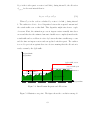
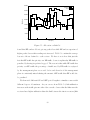
Single Domain with 8 Border Routers and 2 Interior Routers (ST)
81
5.4
Allocation on Link 4-5 . . . . . . . . . . . . . . . . . . . . . . . .
82
5.5
Allocation on Link 5-6 . . . . . . . . . . . . . . . . . . . . . . . .
83
viii
5.6
Single Domain with 24 Border Routers and 9 Interior Routers
(BBN) . . . . . . . . . . . . . . . . . . . . . . . . . . . . . . . . .
86
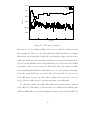
5.7
Allocation on Link 8-6 . . . . . . . . . . . . . . . . . . . . . . . .
87
5.8
Delay of Flow 59-42 . . . . . . . . . . . . . . . . . . . . . . . . . .
87
6.1
Artificial Allocation increase . . . . . . . . . . . . . . . . . . . . .
90
6.2
Inter-Domain protocol message exchanges
. . . . . . . . . . . . .
91
6.3
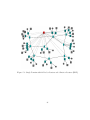
TwoTier Topology . . . . . . . . . . . . . . . . . . . . . . . . . .
93
6.4
Allocation on Inter-domain link 3-11, parameter set 1 . . . . . . .
95
6.5
Allocation on Inter-domain links 3-11, parameter set 2 . . . . . .
96
6.6
Delays for flows 103-216 and 105-223, parameter set 1 . . . . . . .
96
6.7
Delays for flows 103-216 and 105-223, parameter set 2 . . . . . . .
97
7.1
RSVP as an Intra-Domain protocol for source networks . . . . . .
99
7.2
RSVP as an Intra-Domain protocol for destination networks . . . 104
7.3
Propagation of Data . . . . . . . . . . . . . . . . . . . . . . . . . 112
8.1
Implementation Architecture . . . . . . . . . . . . . . . . . . . . . 116
8.2
Forwarding Path Architecture . . . . . . . . . . . . . . . . . . . . 119
8.3
Allocation of resources at the output interface . . . . . . . . . . . 120
8.4
Message Exchange between BB and Edge Routers . . . . . . . . . 124
8.5
Implemetation Topology . . . . . . . . . . . . . . . . . . . . . . . 126
8.6
Incoming traffic from host Camelot . . . . . . . . . . . . . . . . . 127
8.7
Incoming traffic from host Gawain . . . . . . . . . . . . . . . . . . 127
8.8
Outgoing traffic to host Lancelot . . . . . . . . . . . . . . . . . . 128
ix
List of Tables
2.1
Objects Included in Digest Computation . . . . . . . . . . . . . .
27
5.1
Simulation Topologies . . . . . . . . . . . . . . . . . . . . . . . .
79
5.2
Link Speeds . . . . . . . . . . . . . . . . . . . . . . . . . . . . . .
80
5.3
BE and EF Flow Loss Rate (%) . . . . . . . . . . . . . . . . . . .
84
5.4
Link Utilization and Source Burstiness . . . . . . . . . . . . . . .
85
6.1
Topology Characteristics and link speeds . . . . . . . . . . . . . .
94
x
Acknowledgments
I would like to thank my advisor, Lixia Zhang for all the support and guidance
she has given me during the course of my graduate studies. I would also like
to thank my collegues in the UCLA Internet Research Lab and Lan Wang in
particular for all their help.
xi
Vita
1972
Born, Patras, Greece
1995
B.S. (Computer Engineering) University of Patras, Greece
1997
M.Sc. (Computer Science), UCLA, Los Angeles, California.
Publications
• Andreas Terzis, Konstantinos Nikoloudakis, Lan Wang, Lixia Zhang, ”IRLSim: A general purpose packet level network simulator”. Appeared in 33rd
Annual Simulation Symposium, Washington D.C., April 16-20, 2000.
• Andreas Terzis, Lan Wang, Jun Ogawa, Lixia Zhang, ”A Two-Tier Resource Management Model for the Internet”. Appeared in Global Internet
99, Dec 1999.
• Lan Wang, Andreas Terzis, Lixia Zhang, ”A New Proposal for RSVP Refreshes”. Appeared in 7th International Conference on Network Protocols
(ICNP’99), October 1999.
• Andreas Terzis, Jun Ogawa,Sonia Tsui,Lan Wang,Lixia Zhang. ”A Prototype Implementation of the Two-Tier Architecture for Differentiated Services”. Appeared in RTAS99 Vancouver, Canada.
xii
• Andreas Terzis, Mani Srivastava, Lixia Zhang. ”A Simple QoS Signaling
Protocol for Mobile Hosts in the Integrated Services Internet”. Appeared
in INFOCOM99 NY, NY
• Andreas Terzis, Lan Wang, Lixia Zhang. ”A Scalable Resource Management
Framework for Differentiated Services Internet”. Appeared in the third
NASA/NREN Workshop on QoS for the Next Generation Internet.
• Andreas Terzis, Lixia Zhang and Ellen Hahne. ”Making Reservations for
Aggregate Flows: Experiences from an RSVP Tunnels Implementation”.
Appeared in IWQoS’98 Napa Valley, CA.
• Andreas Terzis, Subramaniam Vincent, Lixia Zhang, Bob Braden. ”RSVP
Diagnostic Messages”. RFC 2745
• A. Terzis, J. Krawczyk, J. Wroclaswki, L. Zhang. ”RSVP Operation Over
IP Tunnels”. RFC 2746
• L. Ong, F. Reichmeyer, A. Terzis, L. Zhang, R. Yavatkar. ”A Two-Tier Resource Management Model for Differentiated Services Networks”. Internet
Draft, work in progress
• L. Wang, A. Terzis, L. Zhang. ”RSVP Refresh Overhead Reduction by State
Compression”. Internet Draft, work in progress.
xiii
Abstract of the Dissertation
A Two-Tier Resource Allocation Framework
for the Internet
by
Andreas Terzis
Doctor of Philosophy in Computer Science
University of California, Los Angeles, 2000
Professor Lixia Zhang, Chair
This dissertation research addresses one of the fundamental issues in networking
research: how to provide support for data delivery with assured quality over the
global Internet. The Internet today provides robust, global-scale data delivery
with one single best effort service class. To become the ubiquitous communication
infrastructure of the 21st century, however, the Internet must be enhanced to
effectively support the diverse quality of service requirements of different network
users and applications.
Finding a good solution to this problem is challenging because of the following
two facts: (1) the solution must scale with extremely large numbers of network
users and applications; and (2) the solution must work well in today’s Internet
environment which is made of an interconnection of a large number of networks,
each under different administrative control. Although previous efforts have led
to a rich literature in Quality of Service (QoS) support schemes, most solutions
apply only within limited scope of small networks; none of them have explicitly
addressed the issue of how to control resource allocation across multiple adminis-
xiv
trative domains in order to provide QoS assured end-to-end data delivery across
the global Internet.
In this dissertation research we developed a Two-Tier resource allocation architecture to address the above problems. Following the paradigm of the current
two-tier routing hierarchy, our architecture design divides the resource allocation
in two levels: intra-domain and inter-domain. Intra-domain resource control allocates resources within individual administrative domains according to the traffic
demand. The inter-domain control mechanism is used to coordinate resource
requests and allocations between domains.
Under this architecture, individual administrative domains are free to independently decide what strategies and protocols to choose for internal resource
allocation. At the inter-domain level, aggregate traffic crossing domain borders
is served according to relatively stable, long-lived bilateral service level agreements. The end-to-end QoS support is achieved through the concatenation of
intra-domain resource allocation coupled with bilateral inter-domain agreements
between neighboring domains.
The principal advantages of our Two-Tier architecture design, compared with
previous QoS support mechanisms include drastically improved scaling properties
and a close match to the business reality of the Internet. These benefits however
are associated with a number of new research challenges. Specifically, allocating
resources for traffic aggregates implies that detailed resource requirements along
different network paths are not communicated between domains. Furthermore,
resource allocation in a large system such as the global Internet, requires that
the frequency of re-adjustments must be limited to ensure system stability. To
overcome the lack of information on resource requirements we have developed
a measurement-based approach to estimate QoS traffic directions and allocate
xv
resources inside individual administrative domains. To keep the resource readjustment frequency low in face of rapid changes in traffic load we have devised a
cushion mechanism which inflates the allocation slightly above the actual request
level. The cushion mechanism provides a tool to control the tradeoff between the
level of resource under-utilization and the frequency of allocation re-adjustment.
The same mechanism is used to ameliorate the effects of traffic estimation errors
and shifts in traffic direction.
We have developed a set of intra-domain and inter-domain resource allocation
protocols which implement the Two-Tier architecture. Our simulation results
show that our design can effectively allocate network resources to meet enduser applications QoS requirement, at the same time requires drastically less
state inside the network compared to conventional per-flow resource allocation
approaches. As a proof of concept we have also implemented a partial prototype
of the Two-Tier architecture. This prototype showcases the ability of the TwoTier model to provide end user applications the service assurances they require.
xvi
CHAPTER 1
Introduction
As the Internet matures from a small research network in the 1960’s to the global
commercial infrastructure of the twenty-first century, user needs and expectations
change dramatically. While traditionally the Internet has offered only one level
of service, users already need different services from the network infrastructure.
For example, large corporations want to move their mission critical applications
away from the existing leased lines infrastructure to the public Internet given the
cost reduction, but will only do that when better assurances about the level of
service provided can be guaranteed. The appearance of broadband access technologies (i.e. cable modems and xDSL) coupled with streaming media offerings
from content providers will entice home users to the use of QoS. Along with
traditional network users, the emergence of Voice over IP is driving telecommunication companies (or their competitors) to move their infrastructure away from
the traditional circuit-switched architecture to an IP infrastructure. At the same
time, Internet Service Providers recognize the need for quality network service.
They want to provide their customers the distinct services that will set them
apart from their competitors and give them higher profit margins.
It is the way that these services should be implemented at the network that
brings us to the problem we want to solve. We could state our goal in very few
words as: Define a framework for the provision of service differentiation over the
Internet in a scalable and incrementally deployable way.
1
1.1
The need for Quality of Service Mechanisms
Having established the need for service differentiation in the network we want to
address another question before we begin presenting our solutions to the problem of resource allocation. The question can be roughly formulated as follows:
Given that, with the advent of technologies such as Dense Wavelength Division
Multiplexing (DWDM), bandwidth in the future will be plentiful and therefore
essentially free what is the need for any Quality of Service mechanisms?
One can immediately see that answering this question is essential before we
even begin to work on a resource allocation architecture. If bandwidth is ever
going to be free then there is no need to invent mechanisms that control how it
should be allocated between different network users. However, we believe that
bandwidth is not going to be free in the foreseeable future for several reasons
which we explain next. First of all, even if bandwidth is relatively inexpensive,
service providers will never build a network that cannot return their investment
in terms of building the infrastructure. This means that the utilization of this
network is going to be considerable. Network traffic however is long tailed (see
[WTS95], [LTW93] and [FGW98] among others for evidence and explanation of
this behavior) which means that there are going to be congestion epochs during
which the offered traffic is going to be higher than the network’s capacity. It is
exactly during those congestion epochs that service differentiation is needed.
Our second argument is that there are always going to be regions of the network where bandwidth is going to be less plentiful. Access networks (especially
wireless) fall into this category since technology forecasts show that these networks will have lower capacity for the foreseeable future. Bandwidth at domain
boundaries is also limited but the reasons in this case are not technical but rather
economical. Even in the case were bandwidth is more abundant in the core of
2
the network, resource allocation in the regions where bandwidth is more scarce
is the only way a provider can create the desired service differentiation.
For the reasons mentioned above we believe that resource allocation is going
to be important in future networks providing different levels of service. We now
continue discussing what are the steps in providing the Quality of Service in
future networks.
1.2
Providing Quality of Service
Providing QoS control over the Internet has been a research and engineering
challenge for many years. Achieving QoS in a small, controlled environment seems
simple: if adequate amount of bandwidth either is provisioned or otherwise can
be reserved along the path of a specific data flow, all the packets can be delivered
with minimal transmission delay and no congestion loss. The great challenge
however, is to assure such high performance over the global Internet. One does
observe good performance from time to time when the network is not congested,
but long delays and heavy packet losses are common when the network becomes
heavily loaded. Fundamentally, differentiation of network services requires only
four simple steps:
1. Defining packet treatment classes,
2. Allocating adequate resource to each class at each router,
3. Sorting packets to their corresponding classes and controlling the volume
to be within the allocated amount,
4. Limiting the traffic using the resources allocated to each service class.
3
Over the last three years the Differentiated Services architecture [BBC98] has
emerged trying to address the three points above. By definition, this architecture
contains two main components. The first component includes the fairly wellunderstood behavior in the forwarding path (corresponding to points 1 and 3
above), which is quickly moving through the Internet standardization process.
The second component, corresponding to points 2 and 4 in the list above, involves
the more challenging and largely open, research issues regarding the background
resource allocation component that configures parameters used in the forwarding
path. As we already said before, the topic of scalable resource allocation over the
global Internet is the topic of this thesis.
1.3
Design Goals
The first and foremost goal in our design is scalability. The Internet is expanding at a sustained exponential rate ([RRS98]). Internet backbones run currently
at OC-12 (622 Mbps) and OC-48 (2.4Gbps) speeds, while the introduction of
a OC-192 (10Gbps) is imminent ([Int],[Qwe98]). Any new approach in resource
allocation should therefore aggressively look towards simple solutions suitable for
tomorrow’s even faster, bigger and more complex network. The first step we took
towards achieving the goal of scalability is to adopt a hierarchical design, which
divides resource allocation at two levels: the inter-domain level and the intradomain level. As we describe in Chapter 4, our design specifically limits interdomain resource allocations to be bilateral only, so control overhead can remain
constant when the number of top level Autonomous Systems (AS’s) increases. In
order for resource allocation protocols to scale, no fine granularity information
about individual applications or even about individual client domains should be
propagated through the global network. However to support policy control over
4
resource usage, especially in situations where the network falls into unexpected
resource shortages due to link or node failures, one must keep necessary information regarding the usage of individual client domains, so that one can readjust
the allocation appropriately.
Our second design goal is system simplicity, robustness and responsiveness.
Any new mechanism as critical to network operation as resource management is,
should be very robust to failures and changes in network state.Considering that
down-time translates to lost revenue for ISPs and corporate users, continued operation under any circumstances is critical. Our intra-domain allocation protocol
adopts the soft-state approach to achieve both protocol simplicity and robustness. Following the work we proposed in [WTZ99] we also enhance the soft-state
protocol with acknowledgments for quick loss recovery, thereby improving system
responsiveness.
A commonly cited deficiency for previous QoS architectures was the lack of
mechanisms that associated the improved service that some of the customer’s
packets received, with an increased cost on the customer’s side. ISPs will deploy
QoS only when these mechanisms are in place since this is the only way that they
can protect the investment associated with the deployment of QoS. To keep our
proposal in perspective with the network reality, we want to make sure that our
architecture matches the business model used by Internet Service Providers (ISPs)
for offering network services to their customers. On the other hand, building a
billing architecture is not one of our goals.
Given the current size of the Internet as well as its decentralized administration nature, it is not reasonable to assume that all equipment could be upgraded
overnight to support the architecture we propose in this work. The proposed
solution should be amenable to incremental deployment and should inter-operate
5
as much as possible with other mechanisms for providing QoS as well as legacy
equipment.
1.4
Outline
The rest of this document is structured as follows: In Chapter 2 we present two
mechanisms we have proposed to increase the scalability of the RSVP signaling
protocol. Chapter 3 gives a brief overview of the routing infrastructure in the
Internet today and introduces the Differentiated Services architecture. These two
underlying architectures are discussed since they have influenced the design of the
Two-Tier architecture which we present next in Chapter 4. Chapter 5 elaborates
on the inner workings of the Intra-domain resource allocation protocol, while
Chapter 6 describes the Inter-domain protocol. In Chapter 7 we discuss how the
Two-Tier architecture can be integrated with other solutions to provide end-toend Quality of Service and describe a mechanism for providing feedback on the
state of the network in terms of delay and bandwidth available. Chapter 8 gives an
overview of a partial prototype implementation of the Two-Tier architecture and
in Chapter 9 we discuss about the relative merits of this architecture compared
to other proposals in the area of resource allocation. Finally, we close in Chapter
10 with a summary of our work and a list of future work topics.
6
CHAPTER 2
RSVP Enhancements
2.1
Introduction
In this Chapter we present two proposals for increasing the scalability of the
RSVP signaling protocol used in the Integrated Services architecture. These
two proposals are not directly connected to the Two-Tier resource allocation
architecture which is the main contribution of this work but are related to the
main goal of providing techniques for scalable resource allocation in the global
Internet.
Our starting point for these proposals was as we already said, improving the
scalability of the RSVP signaling protocol (which can be a candidate for the
intra-domain resource signaling protocol in the Two-Tier architecture). There is
however another side effect of this effort: the experience gained from the work
in these two projects influenced the character of the Two-Tier architecture. For
these two reasons we present these two enhancements before we present the TwoTier architecture in the following chapter.
In the sections that follow, we will present the RSVP Tunnels proposal for
encapsulating individual RSVP sessions to larger aggregates as a way of reducing
the amount of RSVP state kept at routers in the core of the network. The second
proposal, involves mechanisms for reducing the overhead of RSVP refreshes as
another way of enabling RSVP to scale. Before we begin though, as a way of
7
introduction we give a brief overview of RSVP.
2.1.1
RSVP
RSVP [ZDE93],[BZB97] is the signaling protocol for the Integrated Services architecture. RSVP is a soft-state, receiver-oriented, two-phase resource reservation
protocol for simplex flows supporting one-to-one and multi-party communication.
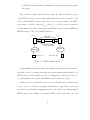
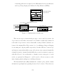
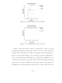
Figure 2.1 provides a representative example of RSVP’s operation.
[rgb]0,0,0PATH
[rgb]0,0,0Sender
[rgb]0,0,0RESV
[rgb]0,0,0Receivers
Figure 2.1: Basic RSVP Operation
Senders advertise the characteristics of the traffic they generate (i.e. in terms
of token buffer parameters), by sending PATH messages to the potential receiver(s). When there are more than one receivers, they are members of a multicast group and senders send their PATH messages to receivers’ multicast group.
Receivers interested in receiving higher QoS send RESV messages requesting a
specific level of service. RESV messages travel on the reverse path from receivers
to senders reserving resources along the way. Receiver orientation matches the Internet multicast model where receivers are responsible for initiating data delivery
and simplifies receiver heterogeneity.
Senders and receivers periodically send their PATH and RESV messages respectively. Routers that do not receive regular refreshes tear down the associated
RSVP state and network resources are released. This approach (Clark in [Cla88]
used the term soft state) provides an elegant yet powerful way of handling net-
8
work failures and stale state. At the same time, periodic refreshes capture very
well the dynamics of large multicast groups where group membership is highly
dynamic.
2.2
2.2.1
RSVP Tunnels
Introduction
IP-in-IP tunnels have become a widely used mechanism for routing packets over
regions of the network that do not implement a particular service (e.g., multicast)
or for augmenting and modifying the behavior of the deployed routing architecture (e.g., mobile IP). Recently IP-in-IP tunneling has been used to implement
Virtual Private Networks (VPNs) over the public Internet. The proposal of providing RSVP support over IP-in-IP Tunnels [TWK00] was born from the need
to support resource reservations over general purpose IP-in-IP tunnels. On the
other hand, RSVP Tunnels can be used to aggregate reservations over the common path shared by a number of individual RSVP flows. The basic idea is to
encapsulate all flows that share the same path with an outer container and then
allocate resources for the container rather than allocate resources for each of the
individual flows.
During the development of the RSVP Tunnels proposal, a number of issues
related to making resource reservations for aggregate data flows became apparent
to us. We believe that these findings are general in nature and are common in
all reservations schemes for aggregate flows.
9
2.2.2
Encapsulation Tunnels
Many large corporations would like to move their networking infrastructure away
from leased lines to the public Internet, as a way of cutting down communication
costs. Virtual Private Networks (VPNs), offered today by most of the nation-wide
Internet service providers, are the response to this market demand.
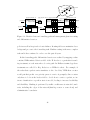
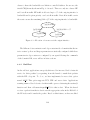
A VPN provides the illusion of a private network overlaid over the public
Internet. In a VPN scenario, as Fig. 2.2 shows, the company’s sites are connected
over the public Internet with virtual links called “tunnels”. Packets that have
to cross sites, enter one end of the virtual link and are transported, through the
common infrastructure, to the other end of the link.
Corporate
Headquarters
Tunnel
Exit Point
Public Internet
Tunnel
Entry Point
Virtual Link
Virtual Link
Telecommuters
Branch Office
Figure 2.2: A Virtual Private Network
The encapsulation technique used in tunneling is fairly simple. An outer IP
header is added in front of the original IP header. This is done by the tunnel
“entry” point as a way to ensure that the packet will first reach the desired
intermediate point specified in the outer destination address, before reaching its
final destination. When the encapsulated packet reaches the tunnel exit point, the
outer header is discarded and the packet is routed towards its final destination.
10
2.2.3
Mechanism Description
From RSVP’s point of view a tunnel, and in fact any sort of link, may participate
in an RSVP-aware network in one of two ways:
1. The (logical) link may not support resource reservation or QoS control at
all. We call this a “best-effort” link.
2. The (logical) link may be able to promise some overall level of level of
resources to carried traffic. Moreover the link may be able to support
reservations for individual end-to-end data flows.
The first type of tunnels exist when some of the routers or the links comprising
the tunnel do not support RSVP. In this case, the tunnel acts as a best-effort link.
The best that we can do is to make sure that the RSVP messages traverse this
logical link correctly, and that the presence of the uncontrolled link is detected.
On the other hand, when the intermediate routers along the tunnel are capable
of supporting RSVP, we would like to have proper resources reserved along the
tunnel to meet clients’ QoS control requests.
Unfortunately, such reservations are not possible with the current IP-in-IP
encapsulation model. Since all the packets that reach one of the tunnel endpoints are encapsulated before being sent to the other side, two main problems
arise:
1. The end-to-end RSVP messages become invisible to intermediate RSVPcapable routers residing between the tunnel end-points.
2. The usual RSVP filters can no longer be used, since data packets are also
encapsulated with an outer IP header, making the original IP (and UDP
11
or TCP) header(s) invisible to intermediate routes between the two tunnel
end-points.
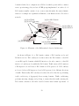
Fig. 2.3 shows a simple tunnel topology, where the senders and the receivers
of an RSVP session are connected through a tunnel between Rentry and Rexit . We
refer to the first RSVP session as the end-to-end or original session. An RSVP
session may be in place between Rentry and Rexit to provide resource reservation
over the tunnel. We refer to this as the tunnel RSVP session, and its PATH and
RESV messages as the tunnel RSVP messages.
Rentry
Tunnel
Rexit
Core Network
Intranet
Intranet
Receiver R1
Sender S1
Figure 2.3: RSVP-Tunnels Model
A tunnel RSVP session may exist independently from any end-to-end sessions.
One may create, for example through some network management interface, an
RSVP session over the tunnel to provide QoS support for data flows from S1 to
R1 , although there is no end-to-end RSVP session between S1 and R1 .
When an end-to-end RSVP session crosses an RSVP-capable tunnel, there
are two cases to consider in designing mechanisms to support the end-to-end
reservation over the tunnel: mapping the end-to-end session to an existing tunnel
RSVP session, and creating a new tunnel RSVP session. In either case, the
12
picture looks like a recursive application of RSVP. The tunnel RSVP session
views the two tunnel endpoints as two end hosts with a unicast Fixed-Filter style
reservation in between. The original, end-to-end RSVP session views the tunnel
as a single (logical) link along the path between the source(s) and destination(s).
The PATH and RESV messages of the end-to-end session are encapsulated at one
tunnel end-point and get decapsulated at the other end, where they get forwarded
as usual.
In both cases, it is necessary to coordinate the actions of the two RSVP sessions, to determine whether or when the tunnel RSVP session should be created
and torn down, and how to correctly map the errors and other reservation related
information from the tunnel RSVP session to the end-to-end RSVP session. The
association between the end-to-end and the tunnel sessions is conveyed through
the SESSION ASSOC object shown in Fig. 2.4.
length
class
c-type
SESSION object
Sender FILTER-SPEC
Figure 2.4: SESSION ASSOC Object
This object is carried by tunnel PATH messages and associates the end-to-end
session described by the SESSION object to the tunnel session described by the
FILTER-SPEC object. As explained below, Rentry encapsulates packets in IP and
UDP headers whose destination address and UDP destination port are the same
for all the tunnel sessions. Hence a tunnel session must be identified primarily
by the UDP source port. The tunnel exit point Rexit , records this association, so
13
that when it receives reservations for the end-to-end session, it knows to translate
them to reservations for the corresponding tunnel session.
Treating the two tunnel end-points as a source and destination host, one can
easily set up a FF-style reservation between them. Now the question is what
kind of filterspec to use for the tunnel reservation, which directly relates to how
packets get encapsulated over the tunnel. We discuss two cases below.
If all the packets traversing a tunnel can use the reserved resources, then the
current IP-in-IP encapsulation could suffice. The RSVP session over the tunnel
simply specifies a FF style reservation with Rentry as the source address and Rexit
as the destination address and zero as source and destination ports.
However if only a subset of the packets traversing the tunnel can use the
reservation, we encapsulate the qualified packets not only with an IP header but
also with a UDP header. This allows intermediate routers to use standard RSVP
filterspec handling without knowing the existence of tunnels. To simplify the
implementation by reducing special case checking and handling, we decided that
all data packets using reservations are encapsulated with an outer IP and a UDP
header. The source port for the UDP header is chosen by the tunnel entry point
Rentry when it establishes the initial PATH state for the new tunnel session. The
destination UDP port used in tunnel sessions is a well known port (363), assigned
by IANA.
2.2.4
Session Association and Error Mapping
In the previous paragraph we presented the SESSION ASSOC object which is
used to associate end-to-end sessions with tunnel sessions. We have already
mentioned two possible associations: mapping all end-to-end sessions to a single
tunnel session, or creating a one-to-one mapping between end-to-end sessions
14
and tunnel sessions. In general, deciding which end-to-end sessions map to which
tunnel sessions is a policy decision that should be left to network managers.
Numerous other modes of aggregation are also possible, for example all traffic for
one service could be aggregated, or all traffic for one customer, etc.
When more than one end-to-end sessions are mapped to the same tunnel
session, then including a “bind” object, that contains the full association, to
every tunnel PATH message may prove to be burdensome. A possible solution
would be to incrementally include and exclude end-to-end sessions to a specific
tunnel session. For example, when Rentry decides that a new end-to-end session
should be mapped to an existing tunnel session, then it includes only this one
in the SESSION ASSOC object, notifying Rexit about this association. When
Rentry wants to remove an end-to-end session from the association it sends a
“negative membership” SESSION ASSOC object to Rexit containing the session
to be removed. A new c-type could be defined for a “negative membership”
SESSION ASSOC object.
As long as the tunnel session is refreshed properly, there is no danger of Rexit
losing the associations between end-to-end and tunnel sessions. For added robustness, it might be desirable that the refresh period for tunnel sessions be
shorter than the one for end-to-end sessions and/or that the tunnel PATH messages include the full association list every K refreshes (where K is the value
defined in [BZB97] as the number of refreshes that can be lost before the session
is timed-out).
Since tunnel sessions “represent” end-to-end sessions in the tunnel, error messages from the tunnel session should be relayed back to the original session.
Specifically, when a tunnel session PATH message encounters an error, it is reported back to Rentry which should relay the error back to the original sender.
15
When Rexit receives a RESV for an end-to-end session, it first sends or refreshes (with possibly changed parameters) the corresponding tunnel RESV message and waits for a confirmation from Rentry that the reservation was successful
before forwarding the end-to-end reservation request. If Rexit immediately forwarded the end-to-end request over the tunnel, then if the tunnel reservation
failed, it would have to explicitly tear down, the installed reservation “past”
Rentry .
When a tunnel session RESV request fails, an error message is returned to
Rexit . Rexit must treat this as an error crossing the logical link and forward the
error back to the receiver.
2.2.5
Scaling Issues
As mentioned in [Bra97], a critical characteristic of any widely deployed QoS
framework is scalability. Quoting from the text: “QoS support must be extensible
eventually from the local network and the campus network through the Gigapop
to the backbone networks and other ISPs”.
Along with scalability, the need for control on the network’s resources from
network managers is identified by the authors of [Bra97] as an equally crucial
characteristic of every QoS framework. Recently, RSVP has been criticized as
lacking both of the above desired characteristics. Some of the arguments used to
support this claim include the following:
• Since the reservations are initiated, from the end hosts, and the reservation
granularity is a source IP address and port number, all the RSVP routers on
the path from the senders to the receivers, have to keep state per sender, per
group. This can burdensome, especially for backbone routers than connect
16
to high speed links, carrying thousands of flows.
• At the same time, network managers cannot configure static reservations
for aggregate flows.
Some authors [GBH97], [BV97], [Boy97], have already tried to identify the
sources of these problems, outlining some possible solutions. In the rest of this
section, we discuss the scaling properties of RSVP reservation over tunnels. We
show that tunnel reservations, when used properly, can substantially reduce the
amount of RSVP control state at backbone routers, reduce the number of RSVP
messages exchanged across backbone routers, as well as provide more control of
the network resources to network managers.
2.2.5.1
State reduction
Using Voice over IP as the candidate service, we can calculate the memory requirements of RSVP in a backbone router. Assuming that every voice flow over
an IP backbone has an RSVP connection a router may have to manage thousands
of flows. For example, if each voice call is using 16 KBps then an OC-3 link can
carry 38875 calls.
Taking into account that the current RSVP implementation from ISI1 uses
around 500 bytes per session, then using the same example as above a backbone
router needs approximately 19 MB to store RSVP related state. In comparison,
today’s routers require approximately 0.7MB to store the full routing table (close
to 80,000 entries).
In the RSVP Tunnels proposal, state aggregation is achieved for backbone
1
The authors of [PS97] quote similar numbers for an implementation of the protocol from
IBM.
17
routers because they do not have to inspect and record state for the end-to-end
RSVP messages, but only for the RSVP messages generated by Rentry and Rexit .
The larger the degree of aggregation at the tunnel endpoints the larger the
gain in reduced RSVP state in the network backbone routers. At one end of
the spectrum, we have individual end-to-end senders getting mapped to different
tunnel senders. Here of course, we have no state reduction in the network backbone routers. At the opposite end of the spectrum, we have the case where all
end-to-end sessions are mapped to a single tunnel sender. In this case we have
the largest amount of state aggregation for routers in the tunnel, since they only
see one aggregate session per tunnel, comprising of all the end-to-end sessions
crossing that tunnel.
2.2.5.2
Reducing the number of messages
Along with the memory requirements, the other source of overhead imposed on
routers from RSVP is the processing of RSVP messages. We will see in Section
2.3 another way to reduce the number of RSVP refresh messages but in the rest
of this section we will see how RSVP Tunnels can help reducing the number of
RSVP messages that have to be created and processed.
Let us consider the RSVP message exchanges for the tunnel sessions. Although end-to-end RSVP messages are still sent through the tunnel, since they
are encapsulated, they are invisible to intermediate routers in the tunnel and
therefore require no RSVP processing.
In the case of tunnel PATH messages, instead of sending every single PATH
message from all the end-to-end senders, Rentry collects the PATH information
from all the senders of end-to-end sessions and sends one PATH message per
tunnel session. The Tspec in the tunnel PATH message is equivalent to the
18
sum of Tspecs of all the senders belonging to end-to-end sessions mapped to the
specific tunnel session.
According to [TWK00], end-to-end RESV messages will trigger a new RESV
message if they represent changes from the originally reserved value. However, if
we change that rule so that the tunnel end points can only send RESV messages
for specific increments (for example only in the order of hundreds of kilobits) then
Rexit could send a new tunnel RESV message only when the aggregate amount
from end-to-end reservations became higher than this threshold value. We call
this scheme, the threshold scheme.
The threshold scheme does not affect the soft-state character of the protocol. After a crash Rexit will have to re-acquire the PATH state and send RESV
messages to restore the amount of reserved resources in any case. Once Rentry becomes alive after the crash, the end-to-end RESV messages will drive the amount
of the tunnel reservations to the level that existed before the crash.
2.2.6
Limitations
While the solution of using RSVP Tunnels to aggregate RSVP sessions over the
core of the network offers a credible solution to the problem of scalability in
resource allocation is still has some fundamental problems that limit its applicability. The biggest limitation is the overhead imposed by having to encapsulate
packets with an outer IP (and UDP) header. This limitation could be ameliorated
by having a more lightweight encapsulation mechanism (e.g. MPLS [CDF99]) but
it can never be totally removed. The second limitation is that tunnel endpoints
have to be statically configured and therefore the mechanism is difficult to adapt
to routing changes. Finally the tunneling mechanism does not address the issue
of inter-domain resource allocation which as we said in Chapter 1 is the most im-
19
portant problem that has to be solved if a QoS architecture is to be commercially
deployed.
We believe that these problems are evidence of the fundamental limitations of
the Integrated Services Architecture and RSVP in particular to provide scalable
resource allocation. These observations were one of reasons that propelled us to
create the Two-Tier resource allocation architecture we present in Chapter 4.
2.3
2.3.1
RSVP Refresh Overhead Reduction
Introduction
In this section we present a mechanism we created for reducing the overhead
created by RSVP refresh messages. As we already said in Section 2.1.1, RSVP is
a soft-state protocol in the sense that all the state established by RSVP messages
has an associated lifetime. RSVP nodes update this state by periodically sending
refresh messages along the data path. If a session’s state is not refreshed, it’s
deleted when its refresh timer expires. Thus the network is free from obsolete or
orphaned reservations.
Refresh messages play the following important roles in assuring correct protocol operation:
1. Automatic adaptation to route changes. Routing changes cause data
flows to switch to different paths. Because RSVP refresh messages follow
the data paths, the first RSVP messages along the new paths will establish
new reservations, while the state along the old path is either explicitly torn
down or automatically timed out.
2. Persistent state synchronization. Since RSVP messages are sent as IP
20
datagrams which can be lost on the way, and RSVP state at individual
nodes may change due to rare or unexpected causes (e.g. undetected bit
errors), periodic refreshes serve as a simple repairing mechanism to correct
any and all inconsistencies in RSVP state along data flow paths.
3. Built-in adaptation mechanism for parameter adjustment. When
either a sender or a receiver needs to change its traffic profile or reservation
parameters during a session, it simply puts these modified parameter values
in the next refresh message.
There is, however, a price to pay for the advantages of simplicity and robustness that come with soft state: the overhead of RSVP refresh messages grows
linearly with the number of active RSVP sessions. Even in the absence of new
control information generated by sources or destinations, an RSVP node sends
one message per active sender-session pair per refresh period to its neighboring
nodes. A related problem is the state setup or tear-down delay caused by the
occasional loss of RSVP messages. Although periodic RSVP refreshes eventually
recover from any previous losses, the recovery delay, which is proportional to
the refresh period, is considered unacceptable for certain applications. One may
consider reducing the recovery delay by reducing the refresh period. Doing so,
would however worsen the refresh overhead problem since refresh messages would
be sent at a higher frequency. To resolve this dilemma we have proposed a new
approach to soft-state overhead reduction by state compression.
The crux of our proposal is to replace all the refresh messages sent between
neighboring nodes for each of the RSVP sessions with a digest message that
contains a compressed “snap shot” of all the shared RSVP sessions between
two neighbor nodes. When an RSVP node, say N, receives a digest from a
neighbor node, it compares the value carried in the digest message with the value
21
computed from N’s local RSVP state. If the two values agree, N refreshes all
the corresponding local state; otherwise N will start the state re-synchronization
process to repair the inconsistency. To assure quick state synchronization we also
enhance RSVP with an acknowledgment option, so instead of waiting for the next
refresh, any lost RSVP messages can be quickly retransmitted.
Before we proceed with our proposed RSVP state compression algorithm we
give the definitions of some terms that will be used in the rest of this section.
RSVP State An RSVP path or reservation state.
Regular/Raw RSVP Message RSVP messages defined in RFC2205 [BZB97],
e.g. PATH, RESV, PathTear and ResvTear messages.
Refresh Message An RSVP message triggered by a refresh timeout to refresh
one or a set of RSVP states. It can be a PATH message for a path state, a
RESV message for a reservation state or a Digest message (in our scheme)
for aggregate state.
MD5 Signature The result of the computation of the MD5 algorithm.
Digest A set of MD5 signatures that represents a compressed version of the
RSVP state shared between two neighboring RSVP nodes.
2.3.2
Design Overview
The goal of our proposal is to improve RSVP’s scalability allowing efficient operation with large number of sessions (e.g. tens of thousands sessions). More
specifically, we aim at reducing the number of refresh messages while still preserving the soft-state approach of RSVP. In this section we briefly describe our
22
state compression approach; the details of the compression scheme are presented
in the next section.
Instead of sending a refresh message per session sender to a neighbor, our
approach is to let each RSVP node send a digest message which is a compact
way of representing all the RSVP session state shared between two neighboring
nodes. In this way, the number of refresh messages sent and processed per refresh
period is reduced from being proportional to the number of sessions to being
proportional to the number of neighbor nodes. Raw RSVP messages are sent
either when triggered by state changes or after state inconsistency is detected to
re-synchronize the state shared between two nodes.
These benefits cannot come without any overhead. Generally speaking, the
protocol overhead of RSVP can be divided into two components, the bandwidth
overhead for message transmissions, and the computation overhead for processing
these messages. One can further subdivide the computation overhead to system
overhead (e.g. system interrupts by packet arrivals) and message processing overhead. The state compression scheme can effectively decrease the bandwidth and
system overhead, however at the cost of increased message processing overhead
as we apply additional processing to compress RSVP state to a single digest message per neighbor. Therefore, one important part of our design is to minimize
the cost of digest computation.
To compress RSVP state into a digest, one can simply concatenate the state
of all the RSVP sessions into a long byte stream and compute a digest over it.
However this brute-force approach suffers from a high overhead of recomputing
the whole digest again whenever any change happens. To scale the digest computation we compute the digest in a structured way. First, we hash all the RSVP
sessions into a table of fixed size. We then compute the signature of each session,
23
and for each slot in the hash table we further compute the slot signature from the
signatures of all the sessions hashed to that slot. On top of this set of signatures,
we build an N-ary tree to compute the final digest (a complete description of the
data structures used is given in section 2.3.3.3).
There are two advantages in using a tree structure to compute the digest:
1. Whenever the digests computed at two neighboring nodes differ, the two
nodes can efficiently locate the portion of inconsistent state by walking
down the digest tree;
2. When an RSVP session state is added/deleted/modified, an RSVP node
only needs to update the signatures along one specific path of the digest
tree, i.e. the branches from the root of the tree to the the leaf node where
the changed session resides.
In our current design, we use the MD5 algorithm to compute state signatures.
As stated in [Riv92], “it is computationally infeasible to produce two messages
having the same message digest, or to produce any message having a given prespecified target message digest.” We can therefore conclude, with a high level
of assurance, that no two sets of different RSVP states will result in the same
signature. However, it should be noted that our state compression scheme can
work well with any hash function that has a low collision probability, such as
CRC-32, as long as two neighboring nodes agree upon their choice of the hash
function.
As a further optimization, we also add an acknowledgment option (ACK) to
the RSVP protocol. The ACK is used to minimize the re-synchronization delay
after an explicit state change request. A node can request an ACK for each
RSVP message that carries state-change information, and promptly retransmit
24
the message until an acknowledgment is received. It is important to note the
difference between a soft-state protocol with ACKs and a hard-state protocol.
A hard-state protocol relies solely on reliable message transmission to assume
synchronized state between entities. A soft-state protocol, on the other hand,
uses ACKs simply to assure quick delivery of messages; it relies on periodic
refreshes to correct any potential state inconsistency that may occur even when
messages are reliably delivered, for example state inconsistency due to undetected
bit errors, or due to undetected state changes.
2.3.3
State Organization
One can suspect that the increase in refresh efficiency cannot come for free. This
is indeed the truth and the trade-off comes in the form of increased storage and
computation. The increase in storage originates from the need to keep per neighbor state, since separate digests are sent to different neighbors. Consequently,
computation costs are inflated since we have to compute the per-neighbor digests
and we have to operate on the per-neighbor data structures.
In the sections that follow we elaborate on the requirements for extra state
introduced by the compression mechanism. Computation costs are further analyzed in Section 2.3.5.
2.3.3.1
Neighbor Data Structure
Current RSVP implementations structure the RSVP state inside a node as a
common pool of sessions, regardless of their destinations. On the other hand,
digest messages sent towards a particular neighbor contain a compressed version
of the RSVP state shared with that neighbor. The need therefore arises to further
organize RSVP state inside a node according to the neighbor(s) each session
25
comes from or goes to. To satisfy this need we introduce the Neighbor data
structure which holds all the information needed to calculate, send and receive
digests to and from a specific node.
In essence the Neighbor data structure is the collection of RSVP sessions that
the current node sends to or receives from a particular neighbor. For efficiency,
neighbor data structures may not actually store the sessions but contain pointers
to the common pool of sessions. This way a session shared with multiple neighbors is not copied multiple times to the corresponding neighbor structures. In
addition to sessions, the neighbor structure contains the digest computed from
the sessions shared with the neighbor and some other auxiliary information such
as retransmission and cleanup timers.
A node needs to compute two digests for each neighbor, one for the state
refreshed by messages received from that neighbor and one for the state the
local node is responsible for refreshing towards that neighbor. We call these two
digests InDigest and OutDigest respectively. OutDigest is sent in lieu of raw
refreshes while InDigest is used to compare whether the local state matches the
state refreshed by that neighbor. In the next section we present how we compress
each session state into an MD5 signature. In section 2.3.3.3 we delve into the
details of the data structure and algorithm we use to derive a digest from the
session signatures.
2.3.3.2
Session Signature
To compress a session state into a signature, we first need to identify which
session parameters need to be constantly synchronized between neighbors. Table
2.1 shows the session objects included in the digest computation. A session is
uniquely identified by a session object which contains the IP destination address,
26
RSVP Objects
Session
PSB
sub-objects to Include
session object
sender template, sender tspec,
adspec, policy
RSB
filterspec, flowspec, reservation style,
policy
Table 2.1: Objects Included in Digest Computation
protocol ID and optionally a destination port number of the associated data
packets. A Path State Block (PSB) is comprised of a sender template (i.e. IP
address and port number of the sender), and a Tspec that describes the sender’s
traffic characteristics and possibly objects for policy control and advertisements.
A Reservation State Block (RSB) contains filterspecs (i.e. sender templates) of
the senders for which the reservation is intended, the reservation style and a
flowspec that quantifies the reservation. It may also contain objects for policy
control and confirmation. Although PSBs and RSBs contain some other fields
such as incoming interface and outgoing interfaces, these fields have only local
meaning to a specific node and therefore should be excluded from the digest
computation. As for RSVP objects defined in the future, the digest computation
can also be applied to them if necessary.
We noticed that, in the current RSVP specification, RSBs record only reservations made on links to downstream neighbors, but not reservation requests
forwarded upstream. However, for a multicast session or many-to-one unicast
session, the reservation request a node receives from a downstream neighbor may
not be the same as the one it sends to an upstream neighbor if the node is a
merging or splitting point. Since the sender of a digest has to compute the digest
based on what flowspec and filterspec are sent to its neighbor, we require such
27
information to be kept in associated RSBs to facilitate the digest computation.
2.3.3.3
Hash Table and Digest Tree
The existence of the structures described in this section is not fundamental for the
correct operation of our compression scheme. However given the context where
our proposed solution will be most useful (e.g. tens of thousands of sessions),
these structures provide the desired performance to make the scheme practically
viable. Two are the principal reasons that compelled us to include these data
structures:
• Given the need for expeditious response to state changes and the high
volatility resulting from the high volume of sessions, updates, insertions
and deletions must be done efficiently. This requirement can be translated
to two subgoals: a data structure that supports efficient session insertions
and deletions and second, incremental digest computation. Unfortunately,
the design of the MD5 algorithm does not allow incremental digest computation. To overcome this limitation we compute the state digest recursively,
by applying the algorithm to session sets of increasing size.
• State inconsistencies must be resolved rapidly without requiring complete
state retransmission. To do so, we need to quickly locate which part of
RSVP state contains the inconsistency and then send raw refreshes only for
these sessions.
In addition to the two primary reasons, simplicity and robustness are essential
if this mechanism is to supersede the minimalism and potency of raw refreshes.
With this set of goals in mind, we continue by presenting each one of the two
data structures next.
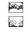
28
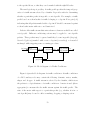
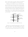
Sessions are stored inside a hash table. The size of the hash table is M
and sessions are hashed to one of the M hash table slots. Hashing is done over
some fixed session fields (e.g the session’s address). If multiple sessions hash
to the same slot, they are inserted in a linked list. Sessions inside the linked
list are stored in-order according to their destination address. Figure 2.5 shows
the session hash table. Slot i contains a pointer to the head of the linked list
of all stored sessions that hash to i. It also contains an MD5 signature that is
computed by concatenating all the sessions’ MD5 signatures and applying the
MD5 algorithm on the compound message.
[rgb]0,0,0Hash Table
[rgb]0,0,0.
[rgb]0,0,0.
[rgb]0,0,0.
[rgb]0,0,0.
[rgb]0,0,0.
[rgb]0,0,0.
[rgb]0,0,0S1
[rgb]0,0,0i
[rgb]0,0,0M
[rgb]0,0,0T /M
[rgb]0,0,0j
Figure 2.5: Hash Table
The second step is to reduce the total number of signatures from M to N,
the number of signatures that can fit inside a single message. To do that we have
introduced a complete N-ary tree whose leaves are the slots of the hash table.
This digest tree is shown in Figure 2.6.
A node constructs the digest tree in the following way: As we said earlier,
the leaves of the tree are the signatures stored in the slots of the hash table. The
signatures of N slots are concatenated and the MD5 algorithm is applied on the
compound message. The result is stored at the parent node on the tree. Looking
at Figure 2.6, signatures x1 , . . . , xN are concatenated and the MD5 algorithm
result is stored in node y1 . This grouping results in M/N level-1 signatures. If
29
[rgb]0,0,0Digest
[rgb]0,0,0...
[rgb]0,0,0h =[rgb]0,0,0y
log M
[rgb]0,0,0...
[rgb]0,0,0...
[rgb]0,0,0...
[rgb]0,0,0...
[rgb]0,0,0...
[rgb]0,0,0N
[rgb]0,0,0x
[rgb]0,0,0x [rgb]0,0,0N
N
1
1
N
[rgb]0,0,0M
Figure 2.6: Digest Tree
the number of level-1 signatures is still larger than N, the node continues on to
group each of N level-1 signatures to compute a level-2 signature to get M/N 2
level-2 signatures. If Ci is the number of level-i signatures, we repeat the grouping
until Ci is less than or to equal to N. The top level signatures represent the digest
of that RSVP state.
We have chosen the degree of the tree to be the same as the maximum number
of MD5 signatures inside the digest object to simplify the data structure and to
reduce the number of parameters. Note that all insertions and deletions are done
in the hash table while the purpose of the digest tree is to reduce the number
of signatures from M to N and to store intermediate results that will be used
during the recovery phase, after inconsistencies are detected.
The hashing table size M and the maximum number N of signatures in a
digest are two important factors that affect the performance of digest computation
and exchange. A larger M means fewer sessions on average hashed to each hash
slot and less overhead in updating a level-1 signature. A large N means possibly
fewer levels in the digest tree and thus fewer messages exchanged during recovery.
In general, one would like M to be comparable to the expected number of active
sessions and N to be the largest value allowed by the link MTU. Furthermore,
30
when the actual number of sessions exceeds the expected number of sessions, the
sender of a digest may choose a higher M and the receiver will need to use the
modified M in its digest computation.
2.3.4
Mechanism Description
2.3.4.1
New RSVP Messages and Objects
Our compression mechanism requires three new RSVP messages, namely: Digest,
ACK and DigestErr. A Digest message carries a timestamp object that uniquely
identifies it and a digest object that represents the state shared between a node
and its neighbor (i.e. the receiver of the message). After a node discovers a
neighbor capable of exchanging digests (see section 2.3.4.2), it periodically sends
Digest messages refreshing the total RSVP state of that neighbor. If a node wishes
to send Digest messages at a different interval than the standard, it can specify
that interval in the Digest message. In this way, the receiver will know when to
expect Digest messages and in their absence when to delete the associated state.
ACK messages are used to acknowledge raw RSVP messages or Digest messages. Since many messages may be outstanding when an ACK is received at
the sender side, the ACK message contains the timestamp of the message it
acknowledges. The receipt of an ACK message indicates that the original message was received and processed by the receiver. Moreover, the message was
processed at the receiver side without creating any errors. Otherwise, an error
message (ResvErr, PathErr or DigestErr) would have arrived instead of the ACK
message.
A DigestErr message acts as a negative acknowledgment to a Digest message.
Similar to ACK messages, the DigestErr message carries the timestamp of the
31
received digest message. In addition, it contains the digest value computed at
the receiver side, which is used later in the recovery process (see section 2.3.4.4).
The timestamp object mentioned before, contains two basic fields: the Timestamp field which is the time that the packet was sent and the Epoch field which is
a random 32-bit value initialized at boot time. All timestamp objects sent from
a node should use the same Epoch value as long as the node is not rebooted.
If, after the initialization phase, a node receives two consecutive messages with
different Epoch values, it can conclude that the sender of these messages has
rebooted. The receiving node must then purge all state associated with that
sender.
We chose to use time as the message identifier because it is always increasing
and so a sender does not have to check if the value is in use or has been used before.
It also helps the receiver to identify which of the RSVP messages for the same
state is the most recent one. However, depending on the node’s processing speed
and timer granularity, two consecutive messages may get the same timestamp
value. Therefore, we define the timestamp to be max(t, tlast + 1), where t is the
current time and tlast is the last timestamp value used.
Furthermore, the timestamp object carries a flag indicating whether the sender
is requesting an acknowledgment for this message. This flag should be turned off
in the timestamp objects carried by ACK and DigestErr messages to avoid an
infinite exchange of ACK messages.
Last, the digest object carries a set of MD5 signatures. These signatures can
be either the digest or some set of MD5 signatures from some other level of the
digest tree.
32
2.3.4.2
Neighbor Discovery
To use the compressed refresh scheme, a node needs to discover which of its
neighbors are capable of exchanging digests. For this reason, when a RSVP
node starts sending (raw) RSVP messages for a session, it should request that
the neighbor(s) acknowledge these messages by including a timestamp object
with the ACK Requested flag turned on. If the node receives an ACK message
in response from a neighbor whose address is not currently on the Neighbor
Structure list, it has then discovered a new compression-capable neighbor. If on
the other hand, that neighbor does not understand timestamp objects (legacy
node), it will return an error message. We can then conclude that this neighbor
is compression-incapable.
When a non-RSVP cloud exists between two RSVP neighbor nodes, although
the nodes can discover each other using acknowledgments during the initial message exchanges, the upstream neighbor may not be able to detect whether sessions
crossing the cloud switch next hops. These changes are caused by route changes
inside the non-RSVP cloud and are not detectable if the upstream neighbor’s
outgoing interface remains the same. The original RSVP specification does not
share this problem since RSVP messages for individual sessions carry the session’s
address and therefore naturally follow any route changes. In the compression
scheme however, digest messages are explicitly addressed to particular next hops
and therefore the same solution cannot be used.
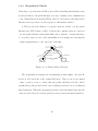
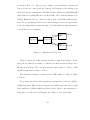
Figure 2.7 illustrates our point. In this scenario node A originally has B as
its downstream neighbor for session D. After a route change, node C becomes
A’s downstream neighbor for that session. However, since A’s outgoing interface
remains unchanged, A will not notice the route change, hence it will continue to
include session D when calculating the digest to B. Node B will not be informed
33
of the change either as long as A sends it the same digest. Therefore, node C will
never get a PATH message from A. As a result, resources will be reserved on the
path between A and B while data packets will follow the path from A to C.
[rgb]0,0,0Original Route [rgb]0,0,0B
[rgb]0,0,0A
[rgb]0,0,0D
[rgb]0,0,0Non RSVP Cloud
[rgb]0,0,0New Route
[rgb]0,0,0C
Figure 2.7: RSVP Session over a non-RSVP cloud
The digest scheme therefore, cannot be used over non-RSVP clouds until an
effective way of detecting route changes is found. Fortunately, the existence of
non-RSVP clouds can be detected by mechanisms described in [BZ97]. If a nonRSVP cloud exists between two nodes, regular refreshes should be used instead
of the compression mechanism.
2.3.4.3
Normal Operation
Neighboring nodes start by exchanging regular RSVP messages as usual. Once
a node discovers a compression-capable neighbor, it creates a digest for the part
of its RSVP state that it shares with each of this neighbors. Subsequently, the
node sends Digest messages instead of raw RSVP refreshes at regular refresh
intervals. When an event that changes the RSVP state (e.g. a sender changes its
traffic characteristics (Tspec)) occurs, raw RSVP messages are sent immediately
to propagate this change.
Raw RSVP messages are sent as before, with the added option of asking
for an ACK. A sender requesting an acknowledgment, includes in the message a
34
timestamp object with the ACK Requested flag turned on. The sender also sets a
retransmission timer for the packet sent. Processing at the receiver side includes
updating the digest of the session that the message belongs to as well as updating
the digest tree. If during processing a condition occurs that requires sending back
an error message back to the sender (e.g a ResvErr) then the receiver sends back
to the sender that error message. This error message will cancel any pending
retransmissions of the original message.
If no ACK is received before the retransmission timer expires, the sender
retransmits the message up to a configured number of times. Each of the retransmissions carries the same timestamp contained in the original message. If
an updated message (i.e. a PATH message from the same sender but with different Tspec) is sent before an ACK is received, the original message becomes
obsolete and no longer needs to be retransmitted. If no ACK arrives even after the message has been retransmitted for the maximum number of times, the
message is purged from the node’s list of pending messages. Any inconsistencies
created by the possible loss of this message will be later resolved by digests.
Digest messages are always sent with the ACK Requested flag turned on.
Digest messages are also retransmitted for a maximum number of times in the
absence of ACK messages. However, following the original RSVP design where
an RSVP node never stops sending refresh messages for each active session, a
node should not stop sending digest refreshes even if it fails to receive an acknowledgment in the previous refresh interval. If the neighbor node crashed and
becomes alive again, it will find the digest value different from its own and the
two routers will start the re-synchronization process. When the digest value is
changed, the node needs to cancel any pending retransmission of the obsolete
Digest message and promptly send a Digest message with the new digest value.
35
When a node receives a Digest message, it checks to see if the state reported
by the Digest message is consistent with the corresponding state stored locally.
To do so the node does a binary comparison between each of the MD5 signatures
contained in the digest object and the corresponding MD5 signatures in the
InDigest (see section 2.3.4.2). If all of them agree then the state is consistent
and an ACK is sent back. Otherwise the receiver returns a DigestErr message
containing its InDigest and the process described in the next section begins.
Figure 2.8 gives an example of message exchanges between two nodes under
normal condition. Nodes A and B had consistent state at time t1 . A sent a Digest
message to B and received an ACK message for it. A then had a state change
at time t2 which triggered a PATH message sent to B. This message was lost, so
A didn’t receive an ACK until it timed out and it had to retransmit the PATH
message (using the same timestamp t2 ). B received the retransmitted PATH
message and sent an ACK message back to A. Up to this point, the two nodes
were synchronized. When the digest refresh timer timed out at t3 , A sent a Digest
message with updated digest value to B. Since A and B were still consistent, B
sent an ACK to A for the Digest message.
2.3.4.4
Recovery Operation
Two RSVP neighbors may become out-of-sync due to a number of reasons. For
instance, a state-changing RSVP message got lost and the sender did not ask for
ACK. It may also happen that a node crashed and lost part or all of its state.
Since it is impossible to enumerate all the possible reasons, the best that one can
do is to detect state inconsistencies once they arise and have a way of repairing
the damaged state.
As we mentioned in section 2.3.4.3, a node sends a DigestErr message if the
36
[rgb]0,0,0Node A[rgb]0,0,0NodeB
[rgb]0,0,0t1
[rgb]0,0,0Digest(t1 )
[rgb]0,0,0Time
[rgb]0,0,0Ack(t1)
[rgb]0,0,0t
[rgb]0,0,0Refresh
2
[rgb]0,0,0PATH(t
2)
[rgb]0,0,0Period
[rgb]0,0,0PATH(t2 )
[rgb]0,0,0Ack(t2)
[rgb]0,0,0t
3
[rgb]0,0,0Digest(t
3)
[rgb]0,0,0Ack(t3)
Figure 2.8: Message Exchange
received digest value disagrees with the local digest. The timestamp and digest
value in the DigestErr message help the two neighbors localize the problem. If
the timestamp acknowledged is smaller than the timestamp of the last Digest
message sent, this error message is for an obsolete message. This message should
be ignored since it may not represent the current state of the neighbor. If they
are equal, the node starts a depth-first search of the mismatching signatures from
the root of the digest tree.
When a node receives a DigestErr message it compares the digest value with
its own to find the states that are inconsistent. When it finds the first mismatching signature (call it S1 ), it sends a Digest message containing the signatures used
to compute S1 . A DigestErr is expected for this Digest message since at least one
of the children signatures should not match. The node again looks for the first
mismatching signature (S2 ) in the second DigestErr message and sends the children of S2 in a Digest message. This procedure is repeated until the leaf signature
(Sh )2 causing the problem is found. Now, the node knows that one or more of
2
h = dlogN M e, see Figure 2.6
37
the sessions in that hash table slot (represented by Sh ) must be inconsistent with
those in the neighbor. It can then locate these sessions by further exchanging
the session signatures with the receiver. However, we found that locating specific
sessions may get quite complicated in some cases, for example, when the sender or
receiver has sessions that do not exist in the peer. When a node encounters these
cases, it can simply send raw refreshes for all the sessions in that particular bin.
After refreshing these sessions, the node re-examines Sh−1 (the parent of Sh ) for
other inconsistencies and continues to traverse the tree until all the mismatching
sessions are located and refreshed.
Notice there is a tradeoff between the latency of the recovery procedure and
the transmission efficiency. For example, if the tree has many levels, many RTTs
are needed to exchange the digests at all the tree levels in order to find the
leaf-level sessions that contribute to the inconsistency. However, if speed of convergence is more important than efficiency, one can stop at an intermediate tree
level and refresh all the states represented by the mismatching signature at that
level.
2.3.4.5
Time Parameters
There are two time parameters associated with digest messages: the refresh period
between successive digest refreshes R and the retransmission timeout T . A node
sends digests at intervals of r, where r is randomly chosen from the range [0.5 ∗
R, 1.5∗R]. Randomization is used to avoid the synchronization of digest messages.
If an acknowledgment is not received after time T from the transmission of a
digest, the node will retransmit that digest message.
The current RSVP specification [BZB97] states that the default refresh period
for regular RSVP messages is 30 seconds but the interval “should be configurable
38
per interface”. To be consistent, digest refreshes are also sent every 30 seconds
by default and this interval should be configurable. As we mentioned in Section
2.3.4.3, digest messages are explicitly acknowledged and therefore there is no
need to decrease R to protect against lost digest messages. However, R affects
the frequency of consistency checking between neighbors, so smaller values of
R should be used in environments where prolonged periods of inconsistency are
unacceptable. The retransmission timeout T should be proportional to the roundtrip time between two directly connected neighbors. A node can measure the time
interval between a message and the corresponding ACK and estimate the mean
RTT by performing exponential averaging on the measurements.
Another important time parameter is the state lifetime L. If state represented
by a digest is not refreshed for a period L, it is considered stale and is deleted.
The naive approach would be to set L to be equal to the refresh period R. This
would however lead to premature state time-outs at the receiving side. There
are at least two reasons for this: first, clocks at neighboring nodes may drift and
second as we said before the refresh timer is randomly set to a value in the range
[0.5 ∗ R, 1.5 ∗ R], which means that the sender may send digests at intervals larger
than R. These examples illustrate that L should be larger than R. Following
the current RSVP specification, we decided to set L = (K + 0.5) ∗ 1.5 ∗ R, where
K = 3.
2.3.4.6
Backward Compatibility
The extensions we have introduced are fully compatible with the existing version
of RSVP. If an RSVP node sends a message with a timestamp object and subsequently receives an “Unknown Object Class” error, it should stop sending any
more messages with attached timestamp object and start using regular refreshes
39
instead of digest refreshes. Digest messages do not pose a compatibility problem
since a node will start sending Digest messages only when it discovers that its
particular peer is compression-capable using the procedure outlined in section
2.3.4.2.
2.3.5
Computation Costs
In this section we focus on the operations applied to the data structures described
in Section 2.3.3 and analyze their requirements in terms of processing.
We begin with some definitions. Let the number of sessions be T , the size
of the hash table be M and the maximum number of MD5 signatures inside
the digest message be N. Let’s further define the cost of computing the MD5
signature of a message of size x to be f (x). To determine the behavior of f (x),
we have to study the algorithm’s behavior. Summarizing the description in RFC
1321 [Riv92], the algorithm divides the input message to 64-byte blocks and
applies a sixty-four step process to each one of these 64-byte blocks. In each
of the sixty-four steps, a number of bit-wise logical operations are applied to
that 64-byte block. The results of the computation on the nth block are used as
input for the computation of the (n + 1)th block. After all the blocks have been
processed, the message’s signature is produced. From this description, one can
see that f (x) is a linear function of x, the size of the input message measured in
bytes.
When a session is modified, a new signature for that session as well as a new
digest of the whole RSVP state has to be computed. To illustrate this procedure,
imagine that we want to update session S1 inside the hash table of Figure 2.5.
First, we look up the session inside the hash table. In our example, we would
come up with the index i. If multiple sessions map to the same hash table slot,
40
we traverse the linked list of sessions until we find the session in question. Once
the session is found and its new MD5 signature is computed, we have to compute
the new MD5 signature stored at the base of the linked list which represents all
the sessions mapped to that hash table slot. On the average dT /Me sessions
will occupy the same slot. The total time needed for this operation is therefore
f (16 ∗ dT /Me), since each MD5 signature is 16 bytes long. The next step is to
update the values on the digest tree. We begin by computing the MD5 signature
of the contents of slot i concatenated with its N − 1 siblings which will be stored
in their parent node on the digest tree. We continue this procedure until we reach
the top of the tree. Since there are dlogN (M)e levels on the tree and at each level
we apply the MD5 algorithm on a message of size 16 ∗ N (the combined size of N
MD5 signatures), the time spent during this step is (dlogN (M)e − 1) ∗ f (N ∗ 16).
Notice that the term is dlogN (M)e−1 since we do not calculate an MD5 signatures
out of the N topmost signatures.
From the discussion above, we can conclude that the total time needed to
calculate the new digest after a session is modified is given by the following
formula, where S is the size of a session in bytes:
f (S) + f (16 ∗ dT /Me) + (dlogN (M)e − 1) ∗ f (N ∗ 16)
(2.1)
When a new session has to be inserted in the hash table, we locate the slot
this session hashes to and insert the session to that slot’s linked list, if one exists.
Given that the list is ordered, the new session has to be inserted in order inside
the list, which means traversing the list until we find a session whose destination
address is larger than the destination address of the session we want to add and
inserting the new session before that session. Deleting a session, involves finding
the slot it hashes to, searching for it inside the linked list, and “splicing” its
predecessor to its successor on the list.
41
The computation cost for the creation of the new digest after an insertion or
deletion operation, is almost identical to the update cost. The only difference is
that in the case of deletion we don’t calculate the MD5 signature of the session
(since we are deleting it). Equations 2.2 and 2.3 respectively, show the insertion
and deletion costs.
f (S) + f (16 ∗ dT /Me) + (dlogN (M)e − 1) ∗ f (N ∗ 16)
(2.2)
f (16 ∗ dT /Me) + (dlogN (M)e − 1) ∗ f (N ∗ 16)
(2.3)
We can see from Equations 2.1, 2.2 and 2.3 that when the size M of the hash
table is small compared to the number of sessions T , the cost of updating the
linked list of sessions will be linear to T . In this case, updating the linked list
becomes the most expensive operation, forcing the total cost to also be linear to
T . The size M of the hash table should therefore be comparable to T to avoid
increased update complexities.
2.3.6
Limitations of our Approach
The ability of two RSVP neighbors to exchange digests in place of raw RSVP
messages relies on the assumption that the two nodes know precisely all the
RSVP sessions that go through these two nodes in sequence. Whenever a route
change occurs, the upstream node must be able to receive a notification from the
RSVP/Routing interface and synchronize the state with the new downstream
node (as well as tear down the session with the old downstream neighbor). For
multicast sessions, another complication arises if a router is attached to a broadcast LAN. A router must detect all changes of membership in the downstream
neighbors, for example when a downstream router on the broadcast LAN joins
or leaves a group, which does not affect the list of outgoing interfaces of the as-
42
sociated RSVP state. Again the proposed scheme relies on the RSVP/Routing
interface to provide notification of such changes.
Furthermore, we have identified two cases where an RSVP node must resort to
the current refresh scheme. The first case is when both compression-capable and
compression-incapable downstream neighbors exist on the LAN. To accommodate the compression-incapable neighbors one must use per session RSVP refresh
messages. The second case is when two RSVP nodes are interconnected through
a non-RSVP cloud as we explained in Section 2.3.4.2.
In summary, a seemingly inevitable limitation of the state compression approach is the loss of RSVP’s automatic adaptation to routing changes. Because
refresh messages for each RSVP session follow the same path as data flow, RSVP
reservation can automatically adapt to routing changes including multicast group
membership changes. When a node compresses the RSVP sessions currently
shared with a neighbor node to a single digest, however, RSVP loses the ability
to trace down the paths of individual flows.
43
CHAPTER 3
Underlying Architectures
3.1
Introduction
In this chapter we will present the two underlying architectures which have influenced the Two-Tier Architecture. The type of reliance is different for each of
these two architectures. For the first one, namely the Internet’s routing architecture, the influence is conceptual since many of the principles first presented
in the routing architecture are also shared by the Two-Tier architecture. On the
other hand for Differentiated Services, which is the second related architecture,
the influence is more technological. What we by this is, that the Two-Tier architecture uses the building blocks created by former architecture as the low level
mechanisms for providing the Quality of Service requested by network users.
In the sections that follow we introduce the two architectures mentioned here
in more detail and explain the ways the Two-Tier architecture relates to them.
3.2
Routing in the Internet
One of the major criticisms for Integrated Services and RSVP is that they require
per-flow state in the network and end-to-end signaling. Result of this criticism
was the search for aggregation schemes in resource reservation. We believe in
this respect, that the evolution of resource management in the Internet closely
44
resembles the evolution of routing protocols that also had to employ aggregation
schemes to cope with exponential increase in routing state as the network’s size
increased. In a similar fashion, routing was the first technology that had to
take into account the administratively diverse nature of the Internet where the
network is a collection of different domains under different administrative control.
For these two reasons, we briefly describe the evolution of the routing architecture
in this section trying to draw any possible analogies.
In the original days of the ARPAnet, all routers had full knowledge of the
network topology and they all participated in the network-wide routing protocol.
As the network grew, memory size needed to keep the routing tables, processing
time needed to update routes and size of routing updates increased substantially.
At the same time, the network had grown administratively diverse, having many
organizational entities wanting to control their own part of the network. Furthermore, given that some of these entities were service providers, they wanted
to hide the internal topology of their network from their competitors.
To address these two problems, the single routing domain of the early network
was replaced by a collection of independent Autonomous Systems (by definition
an Autonomous System (AS for short) is a collection of inter-connected routers
under a single administrative control) connecting to each other. Figure 3.1 shows
such a collection of interconnected ASes.
Each of the administrative domains, or Autonomous Systems, is free to choose
whatever routing protocol that deems proper to run internally (This routing protocol is the Internal Gateway Protocol, or IGP for short). To assure global connectivity, neighboring domains exchange network reachability information using
an Exterior Gateway Protocol (the EGP of choice these days is BGP-4 [RL95]).
One of the features of BGP is that reachability information can be aggregated.
45
[rgb]0,0,0IGP
[rgb]0,0,0AS 1
[rgb]0,0,0AS 2
[rgb]0,0,0Border Router
[rgb]0,0,0BGP
[rgb]0,0,0i-BGP
[rgb]0,0,0AS 3
[rgb]0,0,0AS 4
Figure 3.1: Intra Domain Routing in the Internet
For example, if nearby networks share common address prefixes, then reachability
reports for them can be merged, so a remote site will need to have a single entry
in its forwarding table only for the common prefix.
We believe that any wide-scale resource allocation scheme should recognize
the structure in the Internet today and try to take advantage of it. There are two
characteristics of the routing hierarchy that are specifically relevant to resource
allocation. First, the independence between intra- and inter-domain mechanisms
and second the ability to handle and export information (or in the case of resource
allocation, resources) on different scales, are directly applicable in the resource
allocation scope.
46
3.3
Differentiated Services
The Differentiated Services architecture [BBC98] was conceived by the IETF
community as a way to overcome the shortcomings of Integrated Services in
providing scalable service discrimination in the Internet. This new framework
achieves scalability and flexibility by making a fundamental distinction between
the two components of the architecture:
1. Forwarding Path. This part includes the differential treatment of individual packets at each network node, as implemented by queue service
disciplines and/or queue management disciplines. In addition, the forwarding path may require that some monitoring, policing and shaping be done
on the network traffic designated for “special” treatment.
2. Management Plane. This component includes the co-ordinated configuration of network nodes with respect to which packets get special treatment
and what kind of rules are to be applied to the use of resources.
The division between forwarding path and management plane is beneficial
because it decouples the deployment of the forwarding path elements from the
evolution of the management plane mechanisms. Figure 3.2 shows the division
between the two components of the differentiated services architecture and exposes the resemblance with a similar division followed earlier in the Internet
architecture; the division between forwarding and routing components. Packet
forwarding is the relatively simple task that needs to be performed on a per-packet
basis as quickly as possible. Forwarding uses the packet header to find an entry
in a forwarding table that determines the packet’s output interface. Routing sets
the entries in that table and may need to reflect a range of transit and other
47
[rgb]0,0,0C
[rgb]0,0,0X
[rgb]0,0,0B
[rgb]0,0,0A
[rgb]0,0,0DS Node
[rgb]0,0,0Policies [rgb]0,0,0Node A
[rgb]0,0,0Requests
[rgb]0,0,0Management
[rgb]0,0,0Plane
[rgb]0,0,0Packets
[rgb]0,0,0Forwarding
[rgb]0,0,0Path
[rgb]0,0,0Node B
[rgb]0,0,0RIP
[rgb]0,0,0OSPF
[rgb]0,0,0Routing
[rgb]0,0,0X
[rgb]0,0,0B
[rgb]0,0,04
[rgb]0,0,0Routing
[rgb]0,0,0X
[rgb]0,0,0C
[rgb]0,0,04
[rgb]0,0,0Engine
[rgb]0,0,0Engine
[rgb]0,0,0Packets
[rgb]0,0,0Forwarding
[rgb]0,0,0Forwarding
[rgb]0,0,0X
[rgb]0,0,0B
[rgb]0,0,0C
[rgb]0,0,0Path
[rgb]0,0,0Path[rgb]0,0,0X
Figure 3.2: Division between forwarding path and management plane in routing
and differentiated services
policies as well as keep track of route failures. Routing tables are maintained as a
background process to the forwarding task. Further routing is the more complex
task and it has continued to evolve over the past 20 years.
In the forwarding path, differentiated services are realized by mapping a value
contained Differentiated Services field of the IP header to a particular forwarding treatment, at each network node on its path. In Diffserv terminology these
treatments are called Per Hop Behaviors or PHBs for short. For example, if
the value that a packet carries translates to the “low delay” PHB then a router
would put that packet on a priority queue to service it promptly. Since routers
only have to look at the header field to decide how to service a packet, no intricate classification or per-flow state is needed, leading to increased scalability
and flexibility. Marking is performed by traffic conditioners at network boundaries, including the edges of the network (first-hop router or source host) and
administrative boundaries.
48
Given the mode of operation described above, it is to easy to see that if packets
are marked irrespectively of the amount of underlying resources then the desired
behavior cannot be obtained. The need therefore arises to control the amount of
traffic injected to the network at every service level. This is done in two ways.
First, applications have to request for specific amounts of resources and they
have to get authorization before they can start using them. Usage is policed at
points close to the source where the traffic load is light. Second, if data flows
across domains then resources must also be allocated at the boundaries between
domains. To achieve scalability these resources are allocated in bulk for all the
flows crossing domains and not on a per flow basis. Agreements between domains
on the aggregate amount of traffic crossing the domains’ boundaries are called
Service Level Agreements (SLAs). SLAs represent business agreements and are
supposed to be long lived.
The idea of using a simple bit pattern in the header to specify differentiated
treatment was also used in Frame Relay networks as well as in ATM for the
ABR service. The difference here is that while these networks worked on a perconnection basis, Diffserv applies to aggregates. Also Frame-Relay and ATM are
connection oriented networks, while Diffserv has to work on a connection-less
network making resource allocation more complicated.
3.3.1
Network Elements
In the Differentiated Services architecture the fundamental network entity acting
as a building block for the creation of end-to-end services is a Differentiated Services node. A DS node is a network node (which can be a end-host or a switching
element) implementing at least some of the Per Hop Behaviors. DS nodes are
grouped to administrative entities called Differentiated Services domains. Such a
49
domain is defined as a contiguous set of DS nodes which operate with a common
service provisioning policy and set of PHB groups implemented on each node. A
DS domain normally consists of one or more networks under the same administration; for example an organization’s Intranet or an Internet Service Provider’s
network.
[rgb]0,0,0Traffic
[rgb]0,0,0Conditioning
6
7
[rgb]0,0,0DS Domain
6
7
6
7
6
7
(
)
(
)
*
+
,
-
*
+
(
)
*
+
*
+
(
)
6
7
8
<
9
=
8
<
9
=
$
%
,
-
*
+
(
)
6
7
8
<
9
=
*
+
,
-
$
%
6
7
$
%
*
+
$
%
*
+
(
)
6
7
*
+
6
7
,
-
6
7
(
)
[rgb]0,0,0Ingress
[rgb]0,0,0Router
6
7
6
7
6
7
6
7
*
+
(
)
*
+
*
+
D
E
(
)
6
7
8
<
9
=
8
<
9
=
$
%
8
<
9
=
$
%
$
%
$
%
"
#
,
-
*
+
,
-
8
<
9
=
*
+
(
)
8
<
9
=
*
+
(
)
8
<
9
=
$
%
"
#
*
+
,
-
:
;
*
+
*
+
*
+
"
#
*
+
B
C
"
#
B
C
D
E
(
)
$
%
$
%
*
+
:
;
*
+
:
;
!
!
F
G
!
F
G
!
!
$
%
"
#
,
-
"
#
"
#
*
+
"
#
"
#
*
+
B
C
B
C
:
;
"
#
D
E
(
)
(
)
(
)
!
8
<
9
=
8
<
9
=
$
%
8
<
9
=
$
%
4
5
$
%
4
5
4
5
&
'
4
5
&
'
*
+
,
-
:
;
*
+
:
;
*
+
:
;
!
$
%
<
=
4
5
$
%
*
+
$
%
4
5
$
%
&
'
,
-
*
+
:
;
*
+
:
;
*
+
"
#
*
+
4
5
4
5
&
'
&
'
>
?
2
3
*
+
:
;
*
+
:
;
F
G
!
>
?
>
?
>
?
"
#
.
/
>
?
2
3
*
+
.
/
>
?
@
A
2
3
2
3
*
+
.
/
>
?
2
3
2
3
*
+
.
/
>
?
2
3
2
3
*
+
>
?
2
3
*
+
@
A
*
+
.
/
>
?
@
A
*
+
.
/
>
?
@
A
>
?
@
A
2
3
.
/
*
+
>
?
*
+
>
?
*
+
4
5
[rgb]0,0,0SLA
*
+
:
;
2
3
.
/
>
?
@
A
.
/
2
3
.
/
>
?
@
A
.
/
>
?
@
A
!
@
A
*
+
*
+
:
;
"
#
F
G
!
"
#
*
+
>
?
>
?
>
?
>
?
0
1
B
C
@
A
F
G
!
0
1
!
0
1
"
#
@
A
@
A
0
1
*
+
:
;
D
E
!
0
1
B
C
>
?
0
1
"
#
>
?
:
;
F
G
!
"
#
.
/
F
G
4
5
*
+
0
1
B
C
!
"
#
*
+
&
'
"
#
*
+
4
5
:
;
!
0
1
B
C
"
#
0
1
"
#
*
+
>
?
:
;
!
4
5
:
;
F
G
!
0
1
"
#
&
'
"
#
*
+
:
;
F
G
&
'
[rgb]0,0,0Interior
[rgb]0,0,0Router
"
#
:
;
!
<
=
,
-
!
$
%
&
'
"
#
,
-
<
=
[rgb]0,0,0Egress
[rgb]0,0,0Router
F
G
0
1
@
A
@
A
@
A
@
A
0
1
>
?
[rgb]0,0,0Data
[rgb]0,0,0Upstream
[rgb]0,0,0Domain
[rgb]0,0,0PHB
[rgb]0,0,0Differentiated
[rgb]0,0,0Service
Figure 3.3: Elements of the Differentiated Services Architecture
As shown in Figure 3.3, a DS domain consists of DS boundary nodes and
DS interior nodes. DS boundary nodes interconnect the DS domain to other DS
or non-DS-capable domains, whilst DS interior nodes only connect to other DS
interior or boundary nodes within the DS domain. Traffic enters a DS domain at
a DS ingress node and leaves a DS domain at a DS egress node. DS boundary
nodes act both as a DS ingress node and a DS egress node for different directions
of traffic. Functionally, DS boundary nodes have the added burden of performing
traffic conditioning of (aggregate) flows crossing domains. Traffic conditioning
performs metering, shaping and policing to ensure that the traffic entering the
DS domain conforms to the rules described in the inter-domain agreement. A
50
DS ingress node is responsible for ensuring that the traffic entering a DS domain
conforms to the agreement between it and the upstream domain to which the
ingress is connected. A DS egress node may perform traffic conditioning functions
on traffic forwarded to a directly connected peering domain, depending on the
details of the agreement between the two domains. In what follows we describe
the network elements that accomplish these traffic conditioning functions.
The first part in the process of traffic conditioning is the identification of
packets belonging in particular streams or behavior aggregates. Packet classifiers
select packets in a traffic stream based on the content of some portion of the
packet header. Two types of classifiers are defined:
1. The BA (Behavior Aggregate) classifier, that classifies packets based only
on the value of the DS field in the IP header.
2. The MF (Multi-Field ), classifier selects packets based on the value of a
combination of one or more header fields, such as source address, destination
address, DS field, protocol ID, source and destination port numbers and
other information such as incoming interface.
Given that the classification problem becomes much harder as the number of field
that have to be matched increases, BA classifiers are preferable to MF classifiers,
so one would prefer to have BA classifiers at the domain’s core and position MF
classifiers close to the data sources where the traffic load is lighter. Alas, there
are cases where MF classifiers have to be installed at the edges of domains, such
as the case where a customer’s domain has no DS capabilities but has contracted
a service provider to provide differentiated service to some of its flows. What the
service provider can do is install a MF classifier with filters for the specified flows
at the boundary of the two networks. The classifier identifies packets belonging
51
to the specified flows, so that they can be marked with the right DS value.
The next logical step is profiling. A traffic profile specifies the temporal properties of a traffic stream selected by a classifier. It provides rules for determining
whether a particular packet is in-profile or out-of-profile. For example, a traffic
profile based on a token bucket for traffic belonging to codepoint X is a pair (r, b)
indicating that all packets marked with codepoint X should be measured against
a token bucket meter with rate r and burst size b.
Packets of the traffic stream that arrive when no tokens are available are called
out-of-profile. Different conditioning actions may be applied to out-of-profile
packets. These packets may be queued until they become in-profile (shaping),
discarded (policing) marked with a new codepoint (re-marking) or forwarded
unchanged while triggering some accounting procedure.
[rgb]0,0,0Packets
[rgb]0,0,0Classifier
[rgb]0,0,0Marker
[rgb]0,0,0Shaper/
[rgb]0,0,0Dropper
[rgb]0,0,0Meter
Figure 3.4: Block diagram of a Traffic Conditioner
Figure 3.4 gives the block diagram of a traffic conditioner. A traffic conditioner
of a DS boundary node may contain the following elements: meter, marker,
shaper and dropper. A traffic stream is selected by the classifier, which steers
the packets to a logical instance of a traffic conditioner. A meter is used (where
appropriate) to measure the the traffic stream against the traffic profile. The
state of the meter with respect to a particular packet (e.g., whether it is in- or
out-of-profile) may be used to affect a marking, dropping or shaping action.
52
3.3.2
Per Hop Behaviors
As we said earlier there are two components in the Differentiated Services framework. The first of these components is concerned with defining the treatment
that packets receive in the forwarding path. In this path, differentiated services
are realized by mapping the codepoint contained in the IP packet header to a
particular forwarding treatment, or per-hop behavior (PHB), at each network
node along its path. [NBB98] defines a PHB as: A description of the externally
observable forwarding behavior of a DS node applied to a particular DS behavior
aggregate.
An example of a simple PHB is one which guarantees a minimal bandwidth
allocation of X% of a link to a behavior aggregate. PHBs are expected to be
implemented by employing a range of queue service and/or queue management
disciplines on a network node’s output interface queue. Example of those are
weighted round-robin (WRR) queue servicing or drop-preference queue management. But PHBs are defined in terms of behavior characteristics relevant to
service provisioning policies and not in terms of particular implementation mechanisms.
A replacement header field, called the DS field, is defined in [NBB98], which is
intended to supersede the existing definitions of the IPv4 ToS octet [Pos81a]and
the IPv6 Traffic Class octet [DH98]. The DS field structure is presented below:
[rgb]0,0,00
[rgb]0,0,01
[rgb]0,0,02
[rgb]0,0,03
[rgb]0,0,04
[rgb]0,0,05
[rgb]0,0,06
[rgb]0,0,07
[rgb]0,0,0DSCP
[rgb]0,0,0CU
Figure 3.5: DS Field in IPv4 and IPv6
Six bits of the DS field are used as a codepoint (Differentiated Services Code-
53
point or DSCP) to select the PHB a packet experiences at each node. A two-bit
currently unused (CU) field is reserved and it is supposed to be used for purposes
other than Differentiated Services.
With some exceptions the mapping of codepoints to PHBs is configurable.
Conceptually, there is a configurable mapping from codepoints to PHBs. Even
though specifications of PHBs must include a recommended default codepoint,
in the spirit of every domain being independent, different domains may choose
to use different codepoints for a PHB either in addition or in place of the the
recommended default. If a domain chooses to do so, remarking the DS fields may
be necessary at administrative boundaries even if the same PHBs are implemented
on both sides of the boundary.
PHBs may be specified individually, or as a group (a single PHB is a special
case of a PHB group). A PHB group usually consists of a set two or more PHBs
that can only be meaningfully specified and implemented simultaneously, due to
a common constraint applying to each PHB within the group, such as a queue
servicing or queue management policy. As an example, imagine implementing
drop priority with 4 levels of priority. Then the 4 PHBs needed to define each
of the levels of drop priority would belong to the same drop-priority PHB group.
The DS field in packets requiring a service implemented by a PHB group could
change from one codepoint of the group to some other codepoint in the same
group. Such an action could be taken for example when a flow is out-of-profile.
A PHB group specification should describe conditions under which a packet might
be re-marked to select another PHB within the group.
The structure of the DS field shown above is incompatible with the existing
definition of the IPv4 ToS octet in [Pos81a]. There is although limited backwards
compatibility with current practice in two ways. First, there are per-hop behav-
54
iors that are already in widespread use (e.g., those satisfying the IPv4 Precedence
queuing requirements specified in [Bak95]) and the IETF felt that use of these
behaviors should be allowed with DS-compliant nodes. Second, some codepoints
that correspond to historical use of the IP Precedence and those codepoints were
reserved to map to PHBs having functionality equivalent to the historic use.
Those codepoints are collectively referred as Class Selector Codepoints. For more
on those codepoints, look at [NBB98].
There is a “default” PHB that specifies the common, best-effort forwarding
behavior available in existing routers. A reasonable implementation for this PHB
would be a queuing discipline that sends packets of this class whenever the output
link is not required to satisfy another PHB. A reasonable policy for constructing
services would ensure that the default class was not “starved”. In the paragraph
that follows we present the other two PHBs that have been so far proposed in
the Differentiated Services WF of the IETF.
3.3.2.1
Examples of Per Hop Behaviors
Other that the Default PHB (which corresponds to best-effort service) the Differentiated Services Working Group has defined two other PHBs: the Expedited
Forwarding PHB[JNP99] and the Assured Forwarding PHB [HBW99]. In what
follows, we will briefly talk about these two services as a way of providing examples of per hop behaviors and services that can be constructed from them.
The Expedited Forwarding (EF) PHB was proposed by Van Jacobson et al as
a way of building a low loss, low latency, low jitter and assured bandwidth service
through DS domains. As the authors of [JNP99] explain, loss delay and jitter
are all due to queues that packets experience while going through the network.
Therefore the way to provide low loss, latency and and jitter is to ensure that no
55
(or very small) queues are created on transit nodes. From elementary queuing
theory we know that this can only happen when the (total) arrival rate in a
node, is always smaller than the departure rate. Achieving such a goal requires
two actions: 1. Configuring nodes so that the aggregate EF traffic has a welldefined minimum departure rate (that is independent of other traffic arriving at
the node) and 2. Conditioning the aggregate incoming rate to be always less than
any node’s configured minimum departure rate. The EF PHB tries to provide the
first part while the second part is achieved with mechanisms described in Section
3.3.1 and in later sections. Several types of queue scheduling mechanisms may
be used to deliver the EF PHB. A simple priority queue will give the appropriate
behavior as long as there is no higher priority queue that could preempt the
EF from more than a packet time at the configured rate. Another possible way
suggested, is to used a single queue but a with a weighted round robin scheduler
where share of the output bandwidth assigned to the EF queue is equal to the
configured rate.
In contrast with EF which wants to provide a quantifiable service to Diffserv
customers, Assured Forwarding chooses to define a service in relative terms. The
Assured Forwarding (AF) PHB group [HBW99] is a means for a provider DS
domain to offer different levels of delivery assurances for IP packets received
from a customer DS domain. Four AF classes are defined, where each AF class
has allocated in each DS node a certain amount of forwarding resources (buffer
space, bandwidth). IP packets that wish to use the services provided by the AF
PHB group are assigned by the customer or the provider DS domain into one or
more of these AF classes according to the subscribed services.
Within each AF class IP packets are marked (again by the customer or the
provider DS domain) with one of three possible drop precedence values. In case of
56
congestion, the drop precedence of a packet determines the relative importance of
the packet within the AF class. A congested DS node tries to protect packets with
a lower drop precedence value from being lost by preferably discarding packets
with a higher drop precedence value.
57
CHAPTER 4
The Two-Tier Architecture
The tenet of our design is what we call Two-Tier resource allocation. By this
term we mean that resource allocation should be done in two levels. The first
level is resource allocation inside each administrative domain while the second
level is resource allocation across neighboring domains. Inter-domain resource
allocations are bilateral between neighboring domains. Following the paradigm
of Internet Routing, each domain is free to choose whatever mechanism it wishes
for internal resource management as long as its bilateral resource agreements with
neighboring domains are met.
\
]
\
]
\
]
`
a
`
a
[rgb]0,0,0BBs2
\
]
^
_
\
]
^
_
\
]
^
_
`
a
`
a
b
c
\
]
^
_
b
c
\
]
^
_
b
c
b
c
\
]
^
_
`
a
`
a
[rgb]0,0,0Data Flows
b
c
^
_
^
_
b
c
b
c
^
_
b
c
`
a
`
a
b
c
b
c
b
c
b
c
^
_
^
_
^
_
`
a
`
a
X
Y
d
e
d
e
b
c
b
c
V
W
b
c
Å
^
_
^
_
Ä
V
W
X
Y
V
W
d
e
¶
·
b
c
b
c
b
c
^
_
V
W
b
c
®
¯
X
Y
V
W
X
Y
d
e
¶
·
^
_
Ä
^
_
d
e
[rgb]0,0,0BB2
d
e
b
c
X
Y
X
Y
V
W
V
W
V
W
«
®
¯
^
_
X
Y
X
Y
X
Y
°
±
¼
¼
¼
½
d
e
d
e
¾
¿
À
À
d
e
r
s
Æ
b
c
Æ
b Ç
c
b
c
Ç
Â
Ã
d
e
p
q
r
s
p
q
r
s
p
q
r
s
R
S
R
S
V
W
r
s
V
W
p
q
m
T
U
Z
[
X
Y
T
U
¨
©
T
U
R
S
r
s
r
s
r
s
h
i
r
s
n
o
T
U
¨
©
R
S
Z
R
S
R
S
T
U
Z
[
T
U
n
o
r
s
r
s
h
i
r
s
T
U
[rgb]0,0,0IR2
h
i
Z
t
u
t
u
l
p
q
m
n
o
n
o
l
m
r
s
m
n
o
n
o
n
o
n
o
t
u
n
o
n
o
n
o
n
o
n
o
t
u
l
t
u
l
m
m
n
o
n
o
n
o
t
u
j
v
w
v
w
j
k
v
w
n
o
n
o
N
O
j
k
j
k
v
w
x
y
z
{
z
{
¤
¥
H
I
H
I
H
I
j
v
w
x
y
j
k
[rgb]0,0,0IR1
n
o
¤
¥
H
I
v
w
n
o
t
u
n
o
x
y
t
u
l
[rgb]0,0,0BBs1
x
y
l
z
{
¤
¥
j
v
w
x
y
j
k
v
w
z
{
¤
¥
n
o
n
o
z
{
N
O
f
g
f
g
f
g
f
g
N
O
[rgb]0,0,0BB3
t
u
f
g
n
o
N
O
N
O
N
O
j
k
v
w
x
y
Z
[
T
U
r
s
T
U
n
o
r
s
t
u
l
Z
[
T
U
[rgb]0,0,0Domain 1
[rgb]0,0,0ER1
n
o
r
s
T
U
p
q
m
Z
[
T
U
n
o
r
s
l
p
q
Z
[
T
U
t
u
T
U
h
i
¨
©
t
u
p
q
m
n
o
R
S
T
U
Z
[
Z
ª
l
p
q
m
n
o
Z
[
X
Y
r
s
p
q
m
l
p
q
n
o
Z
[
X
Y
V
W
T
U
r
s
R
S
X
Y
r
s
Z
R
S
T
U
Z
[
T
U
V
W
ª
«
R
S
¨
©
X
Y
V
W
X
Y
T
U
r
s
V
W
r
s
X
Y
r
s
p
q
p
q
Z
R
S
T
U
r
s
X
Y
[rgb]0,0,0Domain 2
V
W
ª
«
R
S
p
q
X
Y
V
W
R
S
R
S
r
s
p
q
V
W
p
q
V
W
ª
«
R
S
[rgb]0,0,0Stub Network
V
W
p
q
[rgb]0,0,0BB1
p
q
r
s
V
W
Ä
d
e
r
s
Ä
Á
d
e
r
s
b
c
Å
Â
f
g
z
{
[rgb]0,0,0Data Flows
[rgb]0,0,0ERS
¦
§
H
I
H
I
H
I
x
y
~
j
k
~
x
y
z
{
N
O
N
O
N
O
H
I
j
~
x
y
j
k
f
g
f
g
f
g
z
{
¦
§
¡
H
I
H
I
H
I
~
x
y
f
g
z
{
f
g
|
}
|
}
¡
L
M
H
I
¡
H
I
¸
H
I
¹
|
}
f
g
f
g
N
O
¬
|
}
|
}
H
I
¡
L
M
¡
H
I
H
I
J
K
L
M
N
O
J
K
È
|
}
x
y
É
È
Ê
Ë
²
³
Ì
J
K
J
K
J
K
J
K
J
K
µ
x
y
È
P
Q
N
O
J
K
H
I
µ
x
y
J
K
P
Q
x
y
¬
P
Q
N
O
J
K
¢
£
f
g
x
y
P
Q
N
O
J
K
H
I
¸
¢
x
y
L
M
J
K
[rgb]0,0,0Domain 3
f
g
z
{
N
O
|
}
N
O
¢
£
~
x
y
N
O
L
M
H
I
¢
~
x
y
N
O
L
M
¡
´
P
Q
P
Q
´
Ì
|
}
|
}
H
I
º
H
I
Î
¸
Î
º
»
¹
H
I
¸
L
M
»
J
K
L
M
J
K
H
I
Ï
Í
L
M
P
Q
J
K
L
M
P
Q
J
K
[rgb]0,0,0IR3
P
Q
[rgb]0,0,0Stub Network
J
K
J
K
J
K
P
Q
J
K
Figure 4.1: Two-Tier Resource Management
While Intra-domain resource allocation can be fined grained (per flow), we
58
require that Inter-domain resource agreements are made for the aggregate traffic
crossing domains. Furthermore, Inter-domain agreements should change infrequently at a larger time-scale than that of individual applications. These two
requirements on Inter-domain agreements provide substantial scaling characteristics by decoupling Inter-domain allocations from individual end-to-end flows.
Figure 4.1 shows how resource allocation information is distributed in the
Two-Tier model. Leaf Domains contact their service providers asking for resources to cover for the aggregate amount of high quality traffic leaving the domain. Once the agreement is in place, individual applications can request and use
portions of the aggregate allocated amount. When and if the allocated resources
are exhausted, the leaf domain may be able to re-negotiate the agreement with
its provider, allocating a larger amount of resources.
Note that the leaf domain only contacts its immediate neighbor for all its
traffic, independent from the traffic’s final destination. It is the responsibility
of the downstream domain, after agreeing to carry the client traffic, to allocate
resources for this traffic both internally but also at its domain boundaries for the
portions of the traffic that exit the domain. The concatenation of intra-domain
management and SLAs between domains creates End-to-End Quality of Service.
4.1
Research Challenges
In order for resource allocation protocols to scale, no fine granularity information
about individual applications or even about individual client domains should be
propagated through the network. The requirement to keep no detailed information introduces however new research challenges that the Two-Tier architecture
has to solve. The domain that receives traffic has to predict where traffic flows
59
to and to make appropriate allocations both internally and externally, since the
upstream domain does not provide any information about the destinations of its
traffic flows. Furthermore each domain that has accepted to carry QoS traffic has
to adapt resource allocations to match shifts in traffic directions. Second, in the
event of a failure, or when sufficient resources are not available to serve the total
amount of traffic, the affected leaf domains should be notified. Given that those
domains do not make explicit requests for traffic going to specific destinations it
becomes harder to notify those domains.
As the authors of [SLC00] have shown, if Inter-domain requests are allowed
to propagate through the domain mesh without control, over time the global allocations can become unstable in a manner that is conceptually similar to route
flapping. We therefore believe that at the inter-domain level the greatest challenge is how we can dampen the request dynamics so the allocation system does
not get into oscillatory behavior.
In the next paragraph we outline the solutions we have proposed to address
the research challenges presented while in the chapters that follow we give in
detail presentation of all the solution components.
4.2
Proposed Solutions
Domains use existing traffic measurements to predict future traffic destinations.
Specifically, ingress routers measure how much traffic entering a domain through
them, exits through each of the domain’s other border routers. Using these measurements ingress routers decide how to divide inter-domain resource allocations
into a number of equivalent intra-domain requests. After an inter-domain request
has been divided to a number of intra-domain requests, these requests are ad-
60
mitted using Measurement Based Admission Control (MBAC) techniques such
as the one present in [JDS95]. We will describe the details of this mechanism in
Sections 5.2, 5.3 and 5.3.1
Our design uses cushions to damp the Inter-Domain resource allocation dynamics and to accommodate errors in the destination estimation process. By
cushion, we mean a safety margin between the request amount and the actual allocation (e.g if the request is for 10 units of bandwidth and 12 units are allocated,
we say that we have a cushion of 2 units of bandwidth). By this mechanism, incremental changes arriving at a domain’s egresses are temporarily ”absorbed”
by the cushion area, giving egresses the ability to delay readjustments of interdomain allocations. The level of cushions is dynamically re-adjusted based on
the observed traffic and request dynamics. We will elaborate on the way cushions
are calculated and their use in Chapters 5 and 6.
The idea of a Bandwidth Broker (BB for short) was first introduced by Van
Jacobson et al in [NJZ99] as the logical entity in charge of resource management
in an administrative domain. Being the locus of control for a domain’s resource
management, the Bandwidth Broker has a dual role:
• Manage the domain’s internal resources. The BB can be responsible
for resource allocation itself or it can delegate resource allocation to an
internal resource management protocol and be responsible only for special
events and policy decisions (e.g. the admission of a new flow.)
• Allocate Inter-domain resources. Each BB maintains bilateral agreements with its neighboring Bandwidth Brokers to allocate resources for the
aggregate amount of traffic crossing domains.
If Inter-domain resource agreements were on a per application-flow basis, the
61
amount of state that would have to be kept by border routers and Bandwidth Brokers would increase linearly with the number of flows crossing domains. Moreover
agreements between domains would have to change very frequently to accommodate for arrivals and departures of individual flows.
Such a behavior would seriously affect the scalability and stability of the
Inter-domain mechanism and of the resource allocation model in general. We
therefore require that resource allocations between domains are for the total aggregate amount of Inter-domain traffic belonging to each service class.
Since Bandwidth Brokers are responsible for resource agreements and resource
agreements are associated with monetary cost it becomes important to protect
Bandwidth Broker communications from malicious attacks. IPsec [KA98] can be
used to provide authentication and confidentiality to messages exchanged between
Bandwidth Brokers. A related issue is how Bandwidth Brokers discover securely
neighboring Bandwidth Brokers and border routers belonging to their domain.
While manual configuration is a first step towards this direction, if the set of
border routers and neighboring Bandwidth Brokers is large and varying, some
discovery mechanism will be required.
For reasons similar to those mentioned about security, robustness is equally
important to the operation of Bandwidth Brokers. As we mentioned before,
the Bandwidth Broker is a logical entity that can map to a single or multiple
physical entities. If the Bandwidth Broker is materialized by multiple physical
entities then robustness is increased (one can imagine a system with one primary
and multiple backup systems implemented BB functionality). This increased
robustness though introduces the problem of consistency between the multiple
physical entities playing the role of the Bandwidth Broker.
An important question related to relationship between neighboring Band-
62
width Brokers, is that of state (and fate) sharing. Depending on the granularity
of resource allocation and negotiation time scales, the amount of state information shared between two BBs may vary. For the sake of robust, fault tolerant
operation, we believe that any sharing of state between BBs should be based on
the soft state model, so that necessary state can be re-established and recovered
quickly when a BB recovers from a crash or a BB is replaced by another one as
part of fault recovery. Therefore, we stipulate that any interaction among BBs
that requires establishment of shared state must involve periodic timeout and
refresh of shared state for robust operation.
63
CHAPTER 5
Intra Domain Protocol
5.1
Introduction
The Intra-Domain protocol serves a dual purpose: First it decides whether to admit or not new Inter-Domain requests performed by a domain’s upstream neighbors and second it periodically adjusts internal allocations to match the shifts in
traffic distribution. The sections that follow present each of the protocol’s tasks
in detail.
5.2
Handling of New Requests
The resource allocation process logically begins when an upstream domain C
sends a resource request to domain P . We will see later in Chapter 6 the details
of Inter-domain messages exchanges, but for now it suffices to say that an external
request reaches domain P . This request is for total projected QoS traffic that the
upstream domain will be sending. The customer domain does not specify the set
of destinations its traffic will flow to. Figure 5.1 represents this situation.
Once the request arrives at domain P , the domain has to decide whether to
admit the request or not. To do so, ingress router I splits the external request to
separate requests towards the domain’s other border routers. The split is done
according to the distribution of the current traffic the ingress sees. Suppose that
64
[rgb]0,0,0E1
[rgb]0,0,0p1 ∗ Rd
[rgb]0,0,0Domain
[rgb]0,0,0I [rgb]0,0,0P
[rgb]0,0,0EC
[rgb]0,0,0Domain
[rgb]0,0,0E2
[rgb]0,0,0C
[rgb]0,0,0p2 ∗ Rd
[rgb]0,0,0Rd
[rgb]0,0,0p3 ∗ Rd
[rgb]0,0,0E3
Figure 5.1: Inter-Domain and Inter-Domain Delta Requests
the request was for Rd units of bandwidth and that I estimates (using the process
described in Section 5.3.1) that p1 percent of traffic goes towards egress router
E1 , p2 percent of traffic goes to egress E2 and p3 percent of traffic goes towards
E3 . I will then send a delta request (it’s called a delta request to differentiate it
from regular requests sent periodically from ingress to egress routers) for p1 ·Rd
to E1 , for p2 ·Rd to E2 and a request for p3 ·Rd to E3 .
Each request message carries a sequence number which has to be unique
among all border routers. In reality if the sequence number field is large enough
(i.e 64 or 128 bits) and ingress routers choose randomly a number from this
sequence space the probability of collision is practically zero. In addition to
the sequence number, each request carries the address of the egress router it is
destined to and is forwarded through the domain traveling towards that egress
router. Requests are forwarded in a hop-by-hop reliable fashion, that is each node
that sends a request message sets a timer and retransmits the request if it does
not receive an acknowledgment before the timer expires. Duplicate requests are
identified by identical sequence numbers.
Interior routers that receive these request messages have to make an admission
decision for the added traffic the messages represent. To do so, an interior router
65
first finds the output link the request will be forwarded through and then checks
whether the current allocation (which is the amount of resources set aside for
existing traffic going out though that link) plus the new request is less than
the maximum amount of resources this traffic class can use. If so, the interior
node forwards the request downstream and increases its allocation by the amount
contained in the request, otherwise it sends a negative response message back to
the ingress router that sent the delta request. Interior routers copy the request’s
sequence number before they forward it, for reasons that we will see later.
Assuming the requests are admitted by all the routers on their path, they will
eventually arrive at the domain’s egress routers. These egress routers perform a
similar check to see whether these requests can be admitted. The admittance test
this time is whether there are enough resources to forward the traffic to the next
domain downstream or not. We will see in Chapter 6 exactly how egress routers
make this decision. For now, it suffices to say that if the new request cannot be
admitted the egress router will try to renegotiate the level of resources allocated
at the boundary with the next downstream domain. On the other hand, if the
new request can be admitted the egress router sends back a positive response
towards the ingress that originally sent this request.
Positive response messages are sent by the egress routers directly to the ingress
that generated the requests. Since response messages sent by the egresses can
be lost, the ingress sets a timeout interval and retransmits its requests if the
responses have not been received before the timers expire. Interior routers that
have already admitted the delta request being retransmitted can detect this by
checking the sequence number in the request against the set of sequence numbers
they have previously received and don’t apply admission control to the duplicate
request. Interior routers purge the list of sequence number they have received at
66
the end of their allocation period (we will see the definition of allocation period
in the next interval) and therefore the amount of state required for sequence
numbers is bounded by the number of the domain’s border routers in the worst
case.
When the ingress router I, that originated the Intra-Domain delta requests
receives replies for all the messages it sent, it can reply back to the upstream
domain. If all the responses were positive, then the ingress also sends back a
positive response and updates its policing rate, otherwise it sends back a negative
response and keeps the policing rate unchanged.
If the ingress router crashes during the time where delta requests are outstanding it will not be able to respond to pending upstream domains’ requests
even if it does receive the response messages. The rebooted ingress router then,
notifies all of it’s exterior neighbors of this failure. Upstream domains should
then try to resubmit their original request after the ingress comes online again.
5.3
Normal Operation
Ingress Routers periodically send Intra-Domain request messages to allocate resources inside the domain for the Inter-Domain requests they have received from
upstream domains. We call these requests refresh or regular requests to differentiate them from delta requests covered in the previous section. The purpose of
these requests is to adjust the allocation levels inside the domain trying to match
the variations in traffic going towards each of the domain’s border routers For
example suppose that in Fig. 5.1, 30% of the traffic entering through I initially
goes towards E1 . Later on this percentage rises to 45% (while the total external
request remains constant). The following refresh request sent by I to E1 will then
67
be for 0.45·Rd.
Ingress routers calculate the request amounts sent in refresh requests by splitting the total external request according to the traffic distribution towards each
of the domain’s other border routers (see Section 5.3.1 for the traffic distribution
estimation). So in our example in Fig. 5.1, router I will send every Ta seconds
(where Ta is the refresh or allocation interval) one request message towards each
other border router it detects is active (i.e. traffic from ingress I goes to that
egress). The requested amount will be the total externally requested amount
multiplied by the estimated percentage of traffic sent towards that egress router.
Refresh request messages also carry the address of the egress router and are forwarded hop-by-hop towards that egress. The same reliability mechanism used for
delta requests is used for refresh requests as well.
Interior routers also divide their time in allocation intervals. For now, let’s
assume that all routers both interior and border have the same allocation interval
Ta (we will see how we can relax this requirement in Section 5.3.2). At the beginning of each allocation period each interior router initializes the total request for
each of it’s outgoing links to zero. For each subsequent refresh request messages
it receives, each interior node increases the total request for the link the message
is forwarded through by the amount contained in the request and forwards the
request downstream towards the egress.
At the end of each allocation interval each interior router must decide how
much resources to allocate on each of its links for the next interval. Allocation
is based on the requested amount but depends also on locally observed network
conditions. The fact that interior routers do not depend entirely on the signals
sent by border routers to make local decisions but also consider information
gathered locally gives our design an added level of robustness against failures. If
68
Ri,j,k is the total request on router i and link j during interval k, the allocation
Ai,j,k+1 for the next interval then is:
Ai,j,k+1 = Ri,j,k + Ci,j,k
(5.1)
Where Ci,j,k is the cushion calculated by router i for link j during interval
k. The cushion’s role is to absorb disparities between the requested amount and
the actual traffic seen on that link. This disparities might arise from a couple
of reasons: First, the estimation process at ingress routers normally introduces
errors and therefore the estimated amount of traffic never completely matches the
actual traffic and second there is a time lag between the time a traffic surge occurs
and the time an ingress router sends an updated refresh request. The cushion
is a node’s protection against those two factors ensuring that the allocation is
rarely overrun by the QoS traffic.
[rgb]0,0,0Traffic
[rgb]0,0,0Rate
[rgb]1,0,0Allocation
[rgb]1,.84,0Request
[rgb]0,0,.82Estimation
[rgb]0,0,0Cushion
[rgb]0,0,0Traffic
[rgb]0,0,0Ta
[rgb]0,0,0Ta
[rgb]0,0,0Ta
[rgb]0,0,0Ta
[rgb]0,0,0Ta [rgb]0,0,0Time
Figure 5.2: Intra-Domain Requests and Allocations
Figure 5.2 illustrates our point. The figure shows the correlation among al-
69
location, request and cushion on a specific link. The total requested amount is
represented by the dashed line, the upper solid line is the allocation while the
lower solid line which is close to traffic volume represents the estimation of the
forwarding path rate. During the first three allocation periods the requested
amount remains constant and the allocation is equal to the requested amount
plus the computed cushion. Approximately at the middle of the third period,
actual traffic rises above the requested amount possibly due to a traffic shift.
The existence of the cushion however, enables the router to successfully serve
the traffic until the end of the third interval where the requested amount is increased. If data traffic had overrun the allocation QoS packets would either have
been buffered or in the worst case dropped.
From the example above, one can see that for cushion to be effective it’s value
should be in the order of the difference between the request level and the actual
traffic rate. With this observation in mind, let’s see now how the cushion Ci,j,k
is calculated in more detail. At the end of each Tf interval (cf. Sec 5.3.1) the
traffic rate estimate fp rate is updated and then the following algorithm is used
to update the cushion:
if(fp_rate > cur_req)
extra = fp_rate - cur_req;
else
extra = 0;
err = extra-avg_cushion;
avg_cushion = avg_cushion + gamma*extra; /* gamma = 1/8 */
dev_cushion = dev_cushion + delta*(abs(err)-dev_cushion);
/* delta = 1/4 */
70
The code fragment above computes the cushion as an exponential weighted
moving average (EWMA) of the positive difference between fp rate and cur req
which is the current request level. This is as we said above is what we are looking
for. Finally, Ci,j,k is equal to avg cushion+beta*dev cushion where beta=2.
From the description so far, one can see that the state requirements for interior
routers are proportional to the number of links each router has. The reason is that
interior routers need to hold information about the current allocation, requested
amount and cushion for each of their adjacent links.
The second role of refresh requests apart from updating allocations on internal
paths is to detect allocation failures. These failures can be the result of either
routing changes or dramatic shifts in traffic distribution. Suppose for example
that an internal link fails and all the traffic previously flowing through that link
has to be re-routed through a different path. It may then happen that the new
path does not have enough capacity to serve the additional traffic routed through
it. Since refresh messages follow the same route as data packets, subsequent
refreshes will flow through the new path raising the request level on nodes on
that path. The interior router where the request level is above the maximum
possible allocation will then send an alert to the domain’s Bandwidth Broker
notifying it about this failure. We will see later on in Section 5.4, how a domain
collectively responds to a failure notification.
Refresh request messages eventually arrive at the domain’s egress routers.
Refresh request messages do not trigger any positive response messages as delta
requests do. We made this design decision since a positive response for refresh
packets does not provide any information to the ingress (to put it another way:
refresh requests are supposed to succeed). The only useful information is that
a refresh was rejected, but this information is delivered by negative response
71
messages from the point of failure.
5.3.1
Traffic Estimation Techniques
Given that upstream domains do not provide any information about the destinations or the current level of injected traffic, domains that have agreed to carry
this traffic have to discover where traffic is headed, check resource availability and
allocate resources on the paths from the point where traffic enters the domain up
to the point where traffic exits the transit network.
Border routers have an enhanced forwarding table, where for each known
destination not only the next hop is listed, but also a set of counters are kept.
Each of these counters counts the number of bytes contained in packets of a
particular service class sent towards that specific destination. Each time that a
packet arrives at an ingress router, the routers looks up the packet’s destination
address in its forwarding table to properly forward the packet towards its next
hop. Additionally, for packets that require higher than best effort service the
ingress router increases the counter associated with that destination.
Once the amount of traffic sent towards each destination in the forwarding
table is measured, the next step is to map destinations to egress routers. For this
task, we assume that each of the border routers participates in the BGP routing
protocol [RL95]. Each BGP router in an Autonomous System, advertises the
destinations learned by exterior peers to all other interior BGP peers in that AS.
Using this information, an ingress router can map each destination to the egress
router used to reach it.
Having this information, ingress routers periodically execute the following
algorithm to compute the amount of traffic sent towards each egress router:
72
for (k=0;k < num_of_BRs;k++) {
egress_router = BR[k];
counter[k] = 0;
for (i=0;i < num_of_destinations;i++) {
if(egress(dest[i]) == egress_router) {
counter[k] += dest[i].counter;
}
}
}
num of destinations is the number of destinations in the router’s forwarding table, num of BRs is the number of the domain’s border routers while the
table BR[...] holds the addresses of the domain’s border routers. The function
egress() returns the egress router towards a destination (by looking at the BGP
routing table). The table dest[i] contains the i-th destination in the forwarding
table, while counter[k] holds the number bytes sent towards egress router k.
The pseudo-code above assumes a single class of service but it is trivial to extend
it to account for multiple classes of service. The only addition required would be
another loop for that collects counters for each of the supported services.
Each ingress router uses the number of bytes sent towards each exit point
during the previous measurement period to calculate the average traffic rate over
the last measurement period. This rate is then used to update the long term
traffic estimate of traffic sent to each of the domain’s egress routers. The traffic
estimation model we have used is a time window measurement process borrowed
from [JDS97], [JB97]. The time window measurement process uses two parameters, Tf and S. Tf is the measurement window and S is the sampling period,
with Tf being a multiple of S. During every sampling period, S, the average rate
mentioned above is computed. The rate estimate, r, is then updated as follows:
73
1. If a newly computed average rate for a given sampling period S is larger
than the current value of r, r is set to the newly computed average.
2. At the end of every measurement window, Tf , r is set to the highest average
rate computed for any S during the previous window.
Increasing Tf increases the amount of history remembered by the measurement process. For a fixed Tf , decreasing S makes this measurement process more
sensitive to bursts of data. Appropriate values of S are likely to be on the order
of thousands of packet transmission times.
5.3.2
Variable Allocation Intervals
In Section 5.3 we used the assumption that all routers use the same allocation
interval Ta . The question that naturally arises then is: What is an appropriate
value for the interval Ta ?
We believe that the only answer to this question
is that there is no single value for Ta which is appropriate for all situations.
Ingress routers that observe frequent traffic fluctuations would like to have a
small Ta value to quickly adapt to the changing conditions, while ingress routers
that observe stable traffic flow could use a large allocation interval value thereby
reducing the protocol’s overhead. In order to accommodate both operational
regimes, we have extended the mechanism described above to include variable
allocation intervals.
Ingress routers adaptively change the allocation interval used for their refresh
messages based on external request variations. The justification for this adaptation algorithm is that when an ingress router observes that its external request
has remained stable for a long time period it gradually increases its Ta replacing
multiple identical refresh requests with a single one that has a larger allocation
74
interval. On the other hand when an ingress router notices variable external
requests it decreases its allocation interval Ta . Furthermore, we want to slowly
increase the allocation internal, while on the other hand we want to quickly respond to changes in external requests. The rationale behind this decision is that
the system has to react slowly to “good news” (the fact that requests are stable) while it has to react fast to “bad news” (in this case the fact that external
requests vary a lot with time). This philosophy is similar to the TCP window
adjusting algorithm using additive increase and multiplicative decrease.
Having these rules in mind we present the adaptation algorithm performed at
ingress I, below:
• I decides what the next allocation interval will be at the end of the current
allocation interval.
• If the external request level has remained stable (by stable we mean that
0.6 ∗ Re ≤ Re0 ≤ 1.2 ∗ Re , where Re0 is the total external request in this
period and Re is the total external in the previous period) for K (e.g.
K = 5) consecutive allocation internals, the ingress additively increases its
Ta by a fixed amount Ti , (Ta0 = Ta + Ti ).
• If Re0 ≥ 1.2 ∗ Re or Re0 ≤ 0.6 ∗ Re then I decreases Ta by a 0.8 multiplicative
factor (Ta0 = 0.8 ∗ Ta ).
• Otherwise, I keeps Ta constant for the next allocation internal.
The complication that arises from using variable allocation intervals is that
interior routers can no longer use the simple update algorithm described in Section
5.3 to calculate the request level at the end of each allocation period. Fortunately
the modifications required are minimal.
75
Requests messages carry, in addition to the requested amount r, the allocation
interval Tr this amount is requested for. Interior routers choose as their allocation
interval the largest Tr value they have seen in the previous interval. Then, when
an interior router i with allocation interval Ti receives a request message for r
for link j it updates the request level Ri,j,k = Ri,j,k + r ∗ (Tr )/(Ti ). For example
suppose that Ti = 3 ∗ Tr , then for each r request Ri,j,k is incremented by r/3.
However, since Ti is 3 times larger than Tr three requests should arrive in a single
Tr interval. One can see then, that at the end of the interval Ri,j,k contains the
requested amount r.
The careful reader at this point may argue that due to delays in requests
arrivals and unsynchronized clocks fewer than Tr /Ti refresh requests can arrive
during an allocation period. The safeguard against these situations is that the total request amount Ri,j,k is not allowed to decrease by more than a multiplicative
factor (e.g 0.8) and so the effect of delayed refresh requests is reduced. Furthermore since the cushion is calculated as the difference between total request and
actual traffic rate the decrease in the request level will be compensated by the
cushion’s increase.
5.4
Reject Behavior
Our discussion so far has been about successful allocations. It is now time to see
how resource allocation failures are handled by our design. The term resource
allocation failure denotes resource requests that cannot be honored because not
enough resources are available. There are at least two reasons why this can
happen: First a physical failure can happen (i.e. a link goes down) or second,
due to a traffic shift more traffic may start traveling towards a new path that
does not have enough capacity.
76
From a domain’s perspective, failures can happen at two different locations:
(1) at an interior router or (2) at the domain’s boundary. Let’s see first what
happens when a failure is detected at an interior node. As we said in Section
5.3 such a failure will be detected when an interior router observes that the total
request on an outbound link is above the maximum possible allocation. At this
point multiple ingress nodes might be using the internal link where the failure
occurred and at least some of them have to be notified about the failure.
In order to find which ingress routers send requests towards the failure point,
the interior router waits until the end of the next allocation interval by when all of
the ingress routers will have sent new requests trying to allocate resources over the
failed path. During this interval, the ingress collects the identities of these ingress
routers and at the end of the next allocation interval sends a failure message
(containing this list of ingresses) to the domain’s Bandwidth Broker. The fact
that the system waits until the end of the next allocation period and does not try
to respond immediately follows the spirit of system where allocation of resources
is done “loosely” without trying to keep tight control over resource allocation.
However loose control does not mean reckless control. The system protects excess
traffic during the time when information is collected by utilizing the cushion set
aside during normal operation. Another way to protect high performance traffic
during this period is to use the bandwidth allocated to best-effort traffic, letting
the best-effort traffic get penalized instead of the high performance traffic.
Once the Bandwidth Broker has been notified, it then consults its Policy
Database to decide which of the ingress routers contained in the failure message
should be notified to reduce their sending rates. For example, if two customers
are affected (because they connect to the ingresses contained in the failure message) and one of them pays a higher price in exchange for higher availability,
77
the domain’s Bandwidth Broker will try to limit the effect on the higher paying customer. In addition to ordering the chosen ingress routers to reduce their
policing rates, the domain’s Bandwidth Broker contacts the affected upstream
peering Bandwidth Brokers to reduce the traffic sent towards the failure point,
which brings us to the second failure scenario: failure at a domain boundary.
In this case, the Bandwidth Broker after receiving the notification from a
downstream domain, it instructs the affected egress router to reduce its sending rate by the amount contained in the notification. Egress routers as interior
routers, keep a list of the ingress routers that have received requests from. So
when an egress router receives a request to reduce its sending rate it forwards a
reply back containing this list of ingress addresses to the domain’s BB which can
then decide (based on the domain’s policy and its agreements with its upstream
neighbors) how much each of the involved ingress routers have to reduce their
sending rate.
In this domain-by-domain manner, failure information is propagated upstream
until it finally reaches the leaf domains that will be ultimately affected by the
resource exhaustion.
5.5
Simulation Results
To validate the design of the intra-domain protocol we have simulated it using a
simulator we have written ourselves. Our simulator is written in PARSEC [Que98]
and is based on a RSVP simulator [TWN98] we had earlier developed. There
are five entities in the simulator: Senders, Border Routers, Interior Routers,
Bandwidth Brokers and Receivers. Senders are the sources of data and receivers
are the final destinations. Interior and Border Routers forward packets according
78
to their service class. In addition, Border Routers are responsible for measuring
data, creating intra- and inter-domain resource allocation messages as well as
shaping and policing traffic. In our simulations we have used the EF PHB as an
example of a service for which resources can be allocated using our protocols. To
implement the EF PHB we have used a priority queue.
To help readers better understand our intra-domain protocol, we first simulate
a single domain with sparse connectivity as shown in Figure 5.3. With this simple
topology (call it ST), we show the relationship among three components of our
intra-domain protocol, i.e. traffic estimation, periodic refreshing of requests, and
resource allocation. We also measured link utilization and loss rate with traffic
sources of different degree of burstiness. The second set of experiments involve a
more realistic topology derived from BBN’s backbone network (Figure 5.6). We
use this topology to verify the conclusions we drew based on the observations
from the simple topology. Moreover, we collected delay and loss statistics to
show the end-to-end services received by receivers. Table 5.1 and 5.2 summarize
the main characteristics of the two topologies.
Topology Border
Core
EF
BE
Receivers
Links
Routers Routers Senders Senders
ST
8
2
8
4
4
33
BBN
24
9
26
0
19
104
Table 5.1: Simulation Topologies
In all the experiments, we use ON/OFF UDP sources. Sources send at constant rate during ON periods and then become silent during OFF periods. To
simulate customer domains where traffic destinations change over time, we switch
the destination of each source at the end of each OFF period (each source has
79
Topology Border-Core Core-Core Access Links
ST
1.5M
5M
1.5M
BBN
1M
10M
250K
Table 5.2: Link Speeds
a list of destinations and they randomly pick one for the next ON period). The
ON and OFF periods are Pareto distributed with shape parameter 1.2 and 1.1
respectively, the same as those of the POO1 sources in [JDS97]. All the sources
start sending traffic at time 0 and continue to send traffic until the simulation
terminates. All the experiments are run for 1000 seconds of simulated time.
As we said before, EF PHB is implemented using a priority queue. The EF
queue is serviced at a rate specified by the management plane. At the end of
each allocation period, the management plane decides how much bandwidth to
allocate for the EF traffic for the next period and it adjusts the service rate of
the EF queue accordingly. The maximum bandwidth that can be allocated for
EF is 40% of the link capacity. Both EF and BE queues have a queue size of 20
packets.
In the ST topology (Figure 5.3), there are two EF senders and one BE sender
connected to each of the four border routers on the left, simulating traffic from
customer domains. Both EF and BE senders send 200-byte packets. As we have
mentioned before, we simulate traffic switching by changing the destination of
packets at the end of each OFF period using a uniform distribution. Since destinations are selected randomly, multiple senders may send to the same receiver
at the same time, resulting in a sudden traffic surge on the links to that particular receiver. Indeed, we have observed such traffic surges in our simulations,
but since our allocation process periodically receives refresh requests that are
80
11
12 S/EF
S/BE
10
BB
19
R
23
S/EF
13
S/EF
14
S/BE
24
S/EF
15
S/EF
16
S/BE
0
BR
1
BR
6
BR
4
IR
5
IR
2
BR
25
S/EF
17
S/EF
8
BR
3
BR
26
18
S/BE S/EF
20
R
7
BR
21
R
9
BR
S/EF: EF Sender
S/BE: BE Sender
R: Receiver
BR: Border Router
IR: Interior Router
BB: Bandwidth Broker
22
R
Figure 5.3: Single Domain with 8 Border Routers and 2 Interior Routers (ST)
adjusted based on traffic estimation, it can quickly adapt its allocation to absorb
the extra traffic.
In the first experiment, we set the ON period to be 860ms and OFF period to
be 140ms. The peak rate for EF senders is 125Kbps and 400Kbps for BE senders.
Figure 5.4 and 5.5 show the estimated traffic rate, the requested bandwidth and
the allocated bandwidth in each allocation period for EF traffic (they are ncur,
tr and alloc respectively in the figures) on two links. As you can see, the traffic
is much smoother on the link from 4 to 5 than that on the link from 5 to 6,
due to a higher degree of multiplexing. One can also observe that the curves
corresponding to requested bandwidth and allocated bandwidth in Figure 5.4
eventually converge. This is because the estimated traffic rate never exceeds
the requested bandwidth. In other words, we do not need a cushion to absorb
extra traffic for this particular link. However, one should note that the cushion
size does not abruptly drop to 0, but it gradually reaches 0, i.e. the cushion
mechanism we use reacts to good news relatively slowly. On the other hand, the
81
1.2e+06
"ncur4-5"
"alloc4-5"
"tr4-5"
1e+06
Rate (bps)
800000
600000
400000
200000
0
0
200
400
600
800
1000
Time (sec)
Figure 5.4: Allocation on Link 4-5
link from 5 to 6 has burstier traffic and we can see that the cushion size has
larger variations. There are a few times when the estimated traffic rate is higher
than the allocated bandwidth, but the allocation quickly adjusts to the increased
traffic rate afterwards. One may suspect that there are packets lost during those
periods, but the simulation traces show that there is no loss for any flows in this
experiment. There are two reasons for this result. First, the estimated traffic
rate is usually higher than the actual traffic rate, so we can actually get warnings
before the actual traffic rate exceeds the allocated bandwidth. Second, as long
as the EF queue does not get full, packets coming in those periods do not get
dropped but are rather queued, experiencing higher delay than usual.
To verify that, under our scheme, EF traffic gets its desired service without
being affected by BE traffic, we increased the rate of BE senders until the sum
of EF and BE traffic exceeded the maximum capacity of the bottleneck link. We
82
350000
"ncur5-6"
"alloc5-6"
"tr5-6"
300000
Rate (bps)
250000
200000
150000
100000
50000
0
0
200
400
600
800
1000
Time (sec)
Figure 5.5: Allocation on Link 5-6
found that EF senders did not get any packet loss while BE senders experienced
higher packet loss as their sending rate increased. Table 5.3 contains the average
loss rate of flows destined to each receiver. We have to note here that just the
fact that EF traffic has priority over BE traffic does not explain why BE traffic is
penalized by having its packets dropped. The reason is that while EF traffic has
priority over EF traffic the percentage of traffic used by EF traffic is configured
by the management plane as we said before and therefore if the management
plane is consistently miscalculating the amount of EF traffic then EF would also
be penalized.
We then tried different ON and OFF period lengths to simulate sources with
different degrees of burstiness. As you can see from Table 5.4, link utilization
increases as the traffic gets smoother. One can also observe that the links near the
receivers have higher utilization than the link between the interior routers (link
83
Receiver
BE Sender’s Rate (Kbps)
19
20
21
22
BE
EF
BE
EF
BE
EF
BE
EF
400
0
0
0
0
0
0
0
0
800
0.9
0
1.8
0
0.9
0
3.7
0
1600
18.9
0 25.5
0
18.4
0 33.2
0
Table 5.3: BE and EF Flow Loss Rate (%)
4–5). This is because all the flows (and requests) go through link 4–5. Recall that
the bandwidth to be allocated for EF traffic on an intra-domain link is the sum
of the requested bandwidth and the cushion size (the cushion size is 0 in this case
as explained before), so the allocated bandwidth on link 4–5 is essentially the
sum of all the senders’ subscribed rates. On the other hand, the links near the
receivers receive requests that match the actual traffic more closely. Figure 5.5
shows that the requested bandwidth is actually lower than the estimated traffic,
because the traffic estimation at internal links is quite conservative (it always
remembers the maximum traffic rate in each time window).
After analyzing the results of the simple topology, we turn to the more complex BBN topology (Figure 5.6). In the following experiments, EF sources send
125-byte packets at 64Kbps with an average ON/OFF period of 300ms/300ms.
Our results show that 73% of the links between interior routers have a utilization higher than 70%. Let’s now look at the resource allocation process. Figure 5.7 shows three curves corresponding to the estimated traffic rate, requested
bandwidth and allocated bandwidth on link 8–6 (other links are similar). It is
consistent with what we saw in Figure 5.5, where traffic is quite bursty and the
allocation curve follows the traffic curve closely to cover traffic surges in a timely
fashion.
84
ON/OFF 500ms/ 750ms/
860ms/ 960ms/
990ms/
500ms
250ms
140ms
40ms
10ms
Link 4–5
0.54
0.55
0.55
0.61
0.77
Link 0–4
0.59
0.62
0.62
0.60
0.63
Link 1–4
0.56
0.56
0.58
0.57
0.63
Link 2–4
0.56
0.55
0.55
0.58
0.60
Link 3–4
0.56
0.59
0.58
0.58
0.64
Link 5–6
0.75
0.82
0.72
0.72
0.76
Link 5–7
0.74
0.76
0.82
0.80
0.83
Link 5–8
0.76
0.76
0.77
0.78
0.81
Link 5–9
0.78
0.75
0.75
0.78
0.82
Table 5.4: Link Utilization and Source Burstiness
What’s more, receivers experienced low loss and low delay jitter in this experiment. We observed the flow from 59 to 42 which goes through 4 interior routers
(router 8, 6, 5 and 1) and 2 border routers (router 24 and 14). Figure 5.8 plots the
packet delay as the simulation proceeds. Analyzing the results from this figure
we find that 93.9% of the packets had a delay of 91 ms while the maximum delay
is 97ms, a 6.6% difference from the minimum.
85
Figure 5.6: Single Domain with 24 Border Routers and 9 Interior Routers (BBN)
86
300000
"ncur8-6"
"alloc8-6"
"tr8-6"
250000
Rate (bps)
200000
150000
100000
50000
0
0
200
400
600
800
1000
Time (sec)
Figure 5.7: Allocation on Link 8-6
0.098
’del42-59’
0.097
Delay (sec)
0.096
0.095
0.094
0.093
0.092
0.091
0
200
400
600
Time (sec)
Figure 5.8: Delay of Flow 59-42
87
800
1000
CHAPTER 6
Inter-Domain Protocol
6.1
Introduction
The function of the Inter-Domain protocol is to adjust Inter-domain allocations
according to changes in traffic distribution and the arrival and departure of new
resource requests originating from leaf domains. These adjustments are however
constrained by two crucial factors: (1) the frequency and sequence of adjustments
has to be regulated if instability is to be contained and (2) the allocation amount
should not be artificially “inflated” (e.g. by adding successive cushions on top
of original requests) as it travels through successive domains. We will see in this
Chapter how our Inter-Domain protocol tries to achieve these two (sometimes
conflicting) goals.
6.2
Protocol Description
Adjustments in Inter-Domain allocations are initiated by an egress router detecting that the amount of resources allocated at the domain boundary with the
downstream domain does not reflect the current request level. There are two
situations when this condition can be triggered.
As we saw in Sections 5.2 and 5.3, delta as well as refresh interior requests are
terminated at the domain’s egress routers. Requests arriving at egress routers
88
are apportioned according to the traffic distribution towards each of the egress’
external neighbors. If the egress then finds that the current traffic level plus
the new request (be it delta or refresh) is above the existing allocation, then a
readjustment is necessary. The level of readjustment is equal to (Fi,j,k + rn ) Ai,j,k , where Fi,j,k is the traffic estimate on the link between egress i and it’s
downstream neighbor j, rn is the new request and Ai,j,k is the current allocation
level.
The second case where a Inter-domain readjustment can occur, is during the
regular refresh cycle used by egress routers. This inter-domain refresh cycle
is decoupled from the intra-domain refresh cycle and is negotiated by the two
external peers. During each refresh cycle an egress router checks for the following
conditions:
e
e
1. If Fi,j,k + Ci,j,k
> Ai,j,k , where Ci,j,k
is the inter-domain cushion that is if the
current traffic estimate plus the cushion is above the allocation, then the
egress requests an increase in the allocation. The additive increase request
e
should be equal to Fi,j,k + Ci,j,k
− Ai,j,k .
e
2. If Fi,j,k + Ci,j,k
< ∗ Ai,j,k , ( ≤ 1 is a constant specifying the low water-
mark threshold ), for M consecutive refresh intervals, the egress requests a
decrease in the inter-domain allocation. We use the hysteresis interval of
M consecutive refresh periods so that decrease requests are sent only when
the existing allocation is persistently higher than the actual request level.
The total new allocation should be equal to the level of actual traffic plus
e
the cushion, that is Fi,j,k + Ci,j,k
.
3. Otherwise, the egress keeps the allocation constant.
At this point the reader will notice that while internally the allocation level
89
is equal to the total amount requested by requests messages plus the cushion, in
domain borders the allocation is equal to the actual traffic rate plus a (different)
cushion. This disparity is indeed intentional and has to do with keeping interdomain allocations from being artificially inflated.
[rgb]0,0,0Rd
[rgb]0,0,0Customer
[rgb]0,0,0Domain
e
00
e
e
[rgb]0,0,0Rd0 = Rd + CA
[rgb]0,0,0R
d = (Rd + CA ) + CB
[rgb]0,0,0rA
[rgb]0,0,0rB
[rgb]0,0,0Provider
[rgb]0,0,0A
[rgb]0,0,0Provider
[rgb]0,0,0B
[rgb]0,0,0Provider
[rgb]0,0,0C
Figure 6.1: Artificial Allocation increase
Fig. 6.1 shows an example of what would happen if Inter-domain requests were
based on intra-domain requests rather than actual traffic estimates. The customer
domain in Fig. 6.1 sends an Inter-domain request Rd . Provider domain A then
creates an intra-domain request r = Rd ,
1
which eventually reaches the egress of
domain A. If this egress was to add it’s cushion CAe on top of the intra-domain
request then it would have to forward an Inter-domain request Rd0 = Rd + CAe .
Similarly the egress of domain B would have to request Rd00 = (Rd +CAe )+CBe . On
the other hand the actual traffic traveling between the chain of domains remains
unchanged and so applying the cushions on top of the traffic estimate to compute
the Inter-domain allocation eliminates the demonstrated potential inflation effect.
The last point we want to make is about the difference between cushions C
and C e applied at interior nodes and domain boundaries respectively. Cushions
at domain boundaries have one extra role in addition to those outlined in Section
5.3. This role is to absorb most new Intra-domain requests. If all Intra-domain
requests were immediately forwarded through domain boundaries then a ripple
1
actually the intra-domain request could be larger than Rd given errors in the traffic distribution estimation process
90
effect would be created in the network leading to the instabilities described in
[SLC00]. For this purpose C e has an additional factor used to compensate for
increases intra-domain requests. We call this new factor the request cushion Cr .
Egress routers keep an exponential weighted moving average of the request deltas
(that is the difference between the total request in the current period and the
previous total request) and Cr is calculated as the mean of the weighted moving
average plus a constant multiple ζ of the variation of this exponential weighted
moving average.
6.3
Inter- and Intra-domain protocol relations
[rgb]0,0,0(6)
[rgb]0,0,0(2)
Ú
Û
Ú
Û
Ú
Û
Ü
Ý
Ü
Ý
Ü
Ý
Ü
Ý
Ú
Û
Ü
Ý
Ú
Û
Ú
Û
Ú
Û
Ü
Ý
Ú
Û
Ú
Û
Ú
Û
[rgb]0,0,0BB1
Ú
Û
Ú
Û
Ü
Ý
Ú
Û
Ú
Û
Ú
Û
Ú
Û
Ú
Û
Ú
Û
Ð
Ð
Ñ
Ü
Ý
Ú
Û
Ü
Ý
Ü
Ý
Ü
Ý
Ú
Û
Ú
Û
Ü
Ý
Ü
Ý
Ð
Ò
Ó
Ò
Ó
Ò
Ó
Ò
Ó
Ò
Ó
Ò
Ó
Ò
Ó
Ò
Ó
Ð
Ñ
Ò
Ó
Ú
Û
Ú
Û
Ú
Û
Ú
Û
Ú
Û
Ú
Û
Ú
Û
Ú
Û
Ú
Û
Ü
Ý
Ð
Ñ
Ò
Ó
Ð
Ú
Û
Ú
Û
Ú
Û
Ü
Ý
Ü
Ý
Ü
Ý
Ð
Ñ
Ò
Ó
Ð
Ú
Û
Ú
Û
Ð
Ñ
Ð
Ñ
Ð
Ñ
Ð
Ñ
Ð
Ñ
Ð
Ñ
Ð
Ñ
Ð
Ñ
Ð
Ñ
Ð
Ñ
Ð
Ñ
Ð
Ñ
Ð
Ñ
Ð
Ñ
Ð
Ñ
Ð
Ñ
Ð
Ñ
Ð
Ñ
Ð
Ñ
Ð
Ñ
[rgb]0,0,0(7) [rgb]0,0,0BB2
[rgb]0,0,0(3)
Ü
Ý
Ð
Ü
Ý
Ð
Ñ
Ü
Ý
Ú
Û
Ð
Ñ
Ò
Ó
Ð
Ñ
Ò
Ó
Ð
Ñ
Ò
Ó
Ð
Ñ
Ò
Ó
Ð
Ñ
Ò
Ó
Ò
Ó
Ò
Ó
Ò
Ó
Ò
Ó
ê
ë
ê
ë
ê
ë
Ü
Ý
Ü
Ý
Ü
Ý
Ü
Ý
Ü
Ý
Ü
Ý
Ú
Û
Ú
Û
Ú
Û
à
á
Ú
Û
Ü
Ý
Ú
Û
Ú
Û
Ü
Ý
Ü
Ý
Ò
Ó
Ò
Ó
Ú
Û
Ú
Û
à
á
Ü
Ý
[rgb]0,0,0(6)
[rgb]0,0,0ER3
[rgb]0,0,0(4)
[rgb]0,0,0Transit
[rgb]0,0,0Network B
[rgb]0,0,0IR1
[rgb]0,0,0(5)
Ð
[rgb]0,0,0(8)
Ú
Û
Ü
Ý
Ú
Û
à
á
Ü
Ý
Ü
Ý
Ú
Û
Ü
Ý
Ð
Ñ
Ò
Ó
Ð
Ò
Ó
Ö
×
Ú
Û
æ
Ü
Ý
Ò
Ó
Ð
Ñ
Ò
Ó
Ö
×
Ö
×
Ð
Ò
Ó
Ú
Û
à
á
Ú
Û
à
á
Ü
Ý
Ú
Û
Ú
Û
Ú
Û
æ
Ü
Ý
Ü
Ý
Ü
Ý
Ø
Ù
Ú
Û
à
á
Ú
Û
à
á
Ü
Ý
Ø
Ù
Ú
Û
Ú
Û
ä
Ü
Ý
Ü
Ý
Þ
ß
Þ
ß
Ú
Û
à
á
Ú
Û
à
á
Ø
Ù
Þ
ß
Ú
Û
Ü
Ý
Ú
Û
Ü
Ý
Ú
Û
Þ
ß
Þ
ß
Ô
Õ
Ö
×
ç
ä
å
Ø
Ù
Þ
ß
Ò
Ó
Ð
Ñ
Ò
Ó
Ö
×
Ô
Õ
Ò
Ó
Ö
×
Ö
×
Ð
Ñ
Ô
Õ
Ö
×
Ð
Ò
Ó
Ú
Û
Ü
Ý
Ø
Ù
Þ
ß
Ö
×
æ
Ø
Ù
Þ
ß
ä
à
á
Ü
Ý
Þ
ß
Ô
Õ
ç
ä
å
Ü
Ý
Þ
ß
Ò
Ó
Ð
Ò
Ó
Ú
Û
Ø
Ù
Ü
Ý
Ø
Ù
[rgb]0,0,0(1)
Ú
Û
à
á
Ü
Ý
Þ
ß
Ö
×
Ú
Û
à
á
Ü
Ý
Ø
Ù
Þ
ß
Ò
Ó
Ô
Õ
Ò
Ó
Ö
×
Ð
Ñ
Ô
Õ
Ö
×
Ð
Ò
Ó
Ú
Û
à
á
Ú
Û
à
á
Ü
Ý
Ú
Û
Ú
Û
Ú
Û
Ú
Û
ä
à
á
Ü
Ý
Ü
Ý
Ü
Ý
Þ
ß
Þ
ß
Ô
Õ
Þ
ß
Þ
ß
Ø
Ù
Ø
Ù
Þ
ß
Ô
Õ
à
á
à
á
Þ
ß
Þ
ß
Þ
ß
Þ
ß
Ø
Ù
Ø
Ù
Þ
ß
Ô
Õ
à
á
à
á
à
á
[rgb]0,0,0ER1
[rgb]0,0,0Transit
[rgb]0,0,0Network A
Þ
ß
à
á
Þ
ß
Þ
ß
Þ
ß
Ø
Ù
à
á
à
á
Þ
ß
Þ
ß
Þ
ß
Þ
ß
Þ
ß
Þ
ß
Ø
Ù
Ø
Ù
Ø
Ù
Ø
Ù
Ø
Ù
Ø
Ù
Ø
Ù
Ô
Õ
Ô
Õ
Ô
Õ
Ö
×
Ö
×
Ö
×
Ò
Ó
Ð
Ñ
Ô
Õ
Ô
Õ
Ô
Õ
Ö
×
Ö
×
Ö
×
Ð
Ñ
Ò
Ó
Ò
Ó
Ò
Ó
Ò
Ó
Ð
Ñ
Ô
Õ
Ð
Ñ
Ô
Õ
Ð
Ñ
Ô
Õ
Ò
Ó
Ò
Ó
Ò
Ó
Ð
Ñ
Ð
Ñ
Ð
Ñ
Ð
Ñ
Ð
Ñ
Ð
Ñ
Ð
Ñ
Ð
Ñ
Ò
Ó
Ò
Ó
Ð
Ñ
Ð
Ñ
Ð
Ñ
Ð
Ñ
â
ã
Ð
Ñ
Ô
Õ
Ð
Ñ
Ô
Õ
Ð
Ñ
Ô
Õ
â
ã
Ô
Õ
â
ã
â
ã
Ð
Ñ
Ô
Õ
Ð
Ñ
â
ã
â
ã
Ð
Ñ
Ô
Õ
Ð
Ñ
Ô
Õ
â
ã
Ô
Õ
â
ã
Ô
Õ
â
ã
â
ã
Ð
Ñ
Ð
Ñ
Ð
Ñ
â
ã
Ð
Ñ
Ð
Ñ
Ô
Õ
Ô
Õ
Ô
Õ
Ô
Õ
Ô
Õ
Ô
Õ
Ô
Õ
Ô
Õ
Ô
Õ
Ô
Õ
Ô
Õ
â
ã
Ô
Õ
â
ã
Ô
Õ
Ô
Õ
Ô
Õ
Ô
Õ
â
ã
Ô
Õ
â
ã
â
ã
Ô
Õ
â
ã
â
ã
Ô
Õ
Ö
×
Ô
Õ
Ö
×
â
ã
â
ã
â
ã
è
é
Ô
Õ
à
á
Þ
ß
à
á
Ö
×
Þ
ß
Ø
Ù
à
á
Ø
Ù
Ò
Ó
Ð
Ñ
Ò
Ó
Ò
Ó
è
é
Ô
Õ
à
á
Þ
ß
Þ
ß
Ø
Ù
Þ
ß
Ø
Ù
Þ
ß
Ö
×
à
á
Ø
Ù
Þ
ß
Ö
×
à
á
Ø
Ù
Þ
ß
Ö
×
ç
ä
å
Ü
Ý
Ø
Ù
Þ
ß
Ð
Ñ
Ò
Ó
Ö
×
Ô
Õ
Ö
×
Ô
Õ
Ö
×
Ô
Õ
Ô
Õ
Ô
Õ
Ô
Õ
â
ã
Ô
Õ
â
ã
â
ã
è
é
Þ
ß
Ô
Õ
Ô
Õ
Ô
Õ
Ô
Õ
Ô
Õ
Ô
Õ
Ô
Õ
â
ã
Ô
Õ
â
ã
â
ã
à
á
Ø
Ù
Þ
ß
Þ
ß
Þ
ß
Þ
ß
Þ
ß
Þ
ß
Þ
ß
Þ
ß
Þ
ß
Þ
ß
è
é
Þ
ß
Ø
Ù
Ô
Õ
Ô
Õ
Ô
Õ
Ô
Õ
Ô
Õ
Ô
Õ
Ô
Õ
Ô
Õ
Ô
Õ
Ô
Õ
Ô
Õ
Ô
Õ
Ô
Õ
Ô
Õ
Ô
Õ
Ô
Õ
Þ
ß
Ø
Ù
Ø
Ù
Þ
ß
Þ
ß
Þ
ß
Þ
ß
Þ
ß
Þ
ß
Þ
ß
Þ
ß
Þ
ß
Þ
ß
Þ
ß
Þ
ß
Þ
ß
Þ
ß
Þ
ß
Þ
ß
Þ
ß
Þ
ß
[rgb]0,0,0ER2
Ø
Ù
Figure 6.2: Inter-Domain protocol message exchanges
Once the egress has decided that an Inter-domain adjustment is required the
sequence of messages shown in Figure 6.2 is executed. We present the sequence
of events required for an increase adjustment but decreases are also similar. The
sequence begins when egress router ER1 notifies BB1 by sending it a message
91
containing the delta Rd between the current allocation and the new increased
inter-domain allocation. BB1 in turn, sends a message to its downstream neighbor BB2 asking for this additional allocation. When BB2 receives this increase
request, it forwards a request to ingress router IR1 querying whether there are
sufficient internal resources to service this increase in entering traffic. The mechanism used by IR1 to make this decision is the one we presented in Section 5.2.
If enough internal resources are available, IR1 replies positively to BB2 , at the
same time adjusting the parameters of it’s policer for incoming traffic from domain A based on the contents of the request. When BB2 receives the positive
reply from IR1 it sends a reply to BB1 accepting the requested increase in traffic.
As a last step then BB1 informs ER1 to increase it’s shaper parameter by Rd .
In the case of a decrease request, steps (4) and (5) would be omitted since no
admission control has to be applied.
6.4
Simulation Results
The purpose of our Inter-Domain simulations is to show how our Inter-domain
protocol can dynamically adjust to changes in traffic crossing domain boundaries
while complying to the constraints we set forth in Section 6.1. Specifically we
want to show how the tuning of inter-domain parameters, such as the cushions
sizes and the hysteresis interval M affect the level and the dynamics of interdomain allocations.
Figure 6.3 shows the topology we have used for our inter-domain simulations. In this topology, traffic sources and destinations are connected to domains
C5, . . . , C15 while Domains 0, . . . , 4 are transit domains. Senders start sending
traffic at time t = 0, 100, 200 and 300 sec and switch destinations at the end
of each ON period. Each source has destinations at different customer domains
92
[rgb]0,0,0s103
[rgb]0,0,0s105
[rgb]0,0,0C6
[rgb]0,0,0C5
[rgb]0,0,0C7
[rgb]0,0,0r216
[rgb]0,0,0Domain
[rgb]0,0,03
0
[rgb]0,0,0C8
[rgb]0,0,0C9
[rgb]0,0,011
[rgb]0,0,0C14
[rgb]0,0,0Domain 1
[rgb]0,0,0Domain 2
[rgb]0,0,0C15
[rgb]0,0,0Domain 3
[rgb]0,0,0Domain 4
[rgb]0,0,0C10
[rgb]0,0,0r223
[rgb]0,0,0C12
[rgb]0,0,0C13
[rgb]0,0,0C11
Figure 6.3: TwoTier Topology
thus creating a traffic variability at the inter-domain level. Table 6.1 shows the
characteristics of the inter-domain topology simulated.
Figures 6.4 and 6.5 present the allocation at the 3-11 inter-domain link for
two sets of inter-domain parameters. In Fig. 6.4 we have used a hysteresis
interval of M = 8 intervals and ζ = 2 (ζ is the multiplicative factor used in
request cushion Cr ) while Fig. 6.5 shows the allocation level for M = 20 and
ζ = 4. The effects of these two parameters on the allocation level are obvious. A
larger hysteresis interval (M = 20) makes the inter-domain allocation more stable
since a longer timer period is required for a decrease operation. For example, in
Fig. 6.4 the allocation level is reduced at t = 890 sec only to be increased
later on. Furthermore using higher requests cushions (Cr with ζ = 4) makes
the inter-domain allocation less sensitive to changes in intra-domain requests.
93
Border Routers 64
Core Routers
23
EF Senders
104
BE Senders
0
Receivers
48
Links
323
Border-Core
10M
Core-Core
15M
Border-Border
4.5M
Table 6.1: Topology Characteristics and link speeds
This effect is clear in Fig. 6.4 where inter-domain readjustments are triggered at
t = 100, t = 200 and t = 300. On the other hand in Fig. 6.5, the request cushion
increases fast during the first interval (t = 0) and stays high. New requests
then arriving at t = 100, 200 and 300 do not trigger inter-domain readjustments.
The downside however is that the inter-domain allocation level in Fig. 6.5 is
higher. The justification is that the cushion keeps the allocation high expecting
possible new increases in intra-domain requests. This cushion however gradually
subsides, as one case see in Fig. 6.5 and eventually the inter-domain allocation
will be reduced.
Figures 6.6 and 6.7 show the effects of the different inter-domain parameters
in application performance. Flow f1 (sender 103 to receiver 216) starts at t = 0
while flow f2 (sender 105 to receiver 223) starts at time t = 100. The delay
perceived by the first flow is initially large since the inter-domain agreements
have not yet been setup. Later on, however f1 ’s delay is virtually constant and
equal to the transmission and propagation delay. When f2 arrives at t = 100,
94
800000
Allocation
Traffic Estimation
Request Cushion
Traffic Cushion
700000
600000
Rate (bps)
500000
400000
300000
200000
100000
0
0
100
200
300
400 500 600
Time (sec)
700
800
900
1000
Figure 6.4: Allocation on Inter-domain link 3-11, parameter set 1
the situation is better since inter-domain resources have been already allocated
and for this reason f2 experiences a smaller initial delay. The difference however
is that in Fig. 6.6 the delay experienced by f1 temporarily increases while reallocations are on the way, while in Fig. 6.7 f1 is practically unaffected.
95
1.2e+06
Allocation
Traffic Estimation
Request Cushion
Traffic Cushion
1e+06
Rate (bps)
800000
600000
400000
200000
0
0
100
200
300
400 500 600
Time (sec)
700
800
900 1000
Figure 6.5: Allocation on Inter-domain links 3-11, parameter set 2
1.4
105-223 Flow
103-216 Flow
1.3
1.2
1.1
Delay (sec)
1
0.9
0.8
0.7
0.6
0.5
0.4
0
100
200
300
400
500
Time (sec)
600
700
800
900
1000
Figure 6.6: Delays for flows 103-216 and 105-223, parameter set 1
96
1.4
105-223 Flow
103-216 Flow
1.3
1.2
1.1
Delay (sec)
1
0.9
0.8
0.7
0.6
0.5
0.4
0
100
200
300
400
500
Time (sec)
600
700
800
900
1000
Figure 6.7: Delays for flows 103-216 and 105-223, parameter set 2
97
CHAPTER 7
End to End Resource Allocation
7.1
Introduction
In the previous chapters we have talked how the intra- and inter-domain protocols
can effectively allocate resources in transit networks, that is networks that are
neither the sources nor the destinations of data traffic. The goal of the TwoTier architecture is however the provision of service differentiation to end-user
applications, so in this chapter we will concentrate on the missing pieces of this
global architecture. Specifically we will discuss how resources can be allocated
at stub networks and how resource allocation in these networks is coupled with
resource allocation in transit networks. In Section 7.3 we are going to discuss the
mechanisms by which feedback information about resource allocation is provided
by the system.
7.2
Resource Allocation in Stub Networks
This section describes how the Two-Tier architecture can be integrated with other
QoS technologies to provide end-to-end Quality of Service support visible to user
applications. In our approach we don’t assume that an end-to-end RSVP session
exists between the source and the destination(s). This approach decouples the resource allocation mechanism used in the source domain from the mechanism used
98
in the destination domain following the guidelines of the Two-Tier architecture.
7.2.1
Source Domain
We look in this paragraph how resources are allocated in the domain where the
source of a traffic flow resides. A host at the source domain that requires for one
of its flows a level of service higher than best effort, starts sending RSVP PATH
messages containing its identification, the flow’s characteristics and the flow’s
destination. The first hop router intercepts those PATH messages and informs
the domain’s Bandwidth Broker about the new request.
[rgb]0,0,0Egress Router
[rgb]0,0,0(3)
[rgb]0,0,0BB
[rgb]0,0,0(2)
[rgb]0,0,0(4) RESV
[rgb]0,0,0First
[rgb]0,0,0PATH
[rgb]0,0,0Hop Router
[rgb]0,0,0(1)
[rgb]0,0,0Host
Figure 7.1: RSVP as an Intra-Domain protocol for source networks
The Bandwidth Broker then takes the following steps:
1. Decides whether the host has the right credentials, according to the domain’s policies to get the request level of service. If not, an error message
is sent back to the host and the whole process stops there.
2. If the request can proceed, the Bandwidth Broker maps the IntServ parameters in the PATH message to the appropriate Diffserv parameters. For
example, Guaranteed Service could be mapped to the EF PHB while the
Controlled Load service could be mapped to (some level of) AF.
99
3. Based on these parameters and the flow’s destination, the Bandwidth Broker decides if there are enough inter-domain resources available.
If enough resources are available, then the Bandwidth Broker instructs the
first hop router to forward the PATH message. The BB also informs the appropriate egress router to increase the total amount of traffic crossing the domain
by the requested amount and to start producing RESV messages for the host’s
flow. If on the other hand, the new flow cannot be admitted without violating the inter-domain agreement, then based on the type of SLA between the
two domains (static vs. dynamic) the Bandwidth Broker may request additional
resources from the downstream domain. If the resources are granted then the
request proceeds as in the case above, otherwise an error message is sent back to
the sending host.
Once the egress router receives the PATH message, it starts sending RSVP
RESV messages upstream towards the sender. PATH messages do not flow
through outside the domain but are terminated at the egress router. The RESV
messages reserve resources on the path from the egress router to the sending
host. If at some point on the path not enough resources are available then an
error message will be sent back to the egress router. In this case the egress router
notifies the Bandwidth Broker. The BB can in turn notify the sender about this
failure.
The reception of a RESV message from the first hop router is an indication
that resources have been reserved on the path to the egress router. There are
two possible next steps 1 :
• If the mapping between IntServ and Diffserv parameters is fixed, then based
1
We assume here that the first hop router is responsible for setting the DS field. We describe
another solution in the following section
100
on the parameters in the PATH message a filter can be set to recognize
packets belonging to the new flow. Packets belonging to this flow will be
stamped with the appropriate DS value and will be policed to the level
advertised by the source in its PATH messages.
• Otherwise, the first hop router receives the mapping between IntServ and
Diffserv parameters as part of the response by the Bandwidth Broker in the
first step described above.
7.2.1.1
Source Marking
In the previous section we said that the first hop router is responsible for setting
the DS field of application packets. An alternative is to have the source host to do
the marking instead. While this assumes that source hosts have this capability,
there are considerable advantages in source marking:
• Since the hosts are marking the packets, no MF classifiers are needed at
first hop routers leading to better scaling properties.
• The first hop router may not be able to identify specific application flows
based on network and/on transport layer fields in the packet. For example,
consider the case of encrypted traffic flows (IPSec) where transport layer
fields are not visible to the first hop router.
• Applications can mark their packets using knowledge that is not available
to first hop routers. For example, an application that stamps packets with
codepoints from the AF group can selectively decide which packets receive
the lowest drop priority based on application semantics, while the first hop
router could pick arbitrary application packets as long as the right amount
of packets is being stamped with the lowest drop priority.
101
The fact that the source host is marking packets does not mean that the first
hop router is relieved from all of its duties. It will still have to use policing to
make sure that hosts do not send more traffic at a specific PHB level, than what
they have asked for.
7.2.2
Destination Domain
At the destination domain, we have a similar goal of trying to allocate resources
from the domain’s ingress to the destination host. Our scheme works as follows:
the ingress router of the Destination domain starts sending PATH messages towards the final destination. The destination host responds by sending RESV
messages reserving the needed resources inside the destination domain.
There are two issues here. First, how does the receiving host at the destination
domain learn about the sending host and the characteristics of the flow it is
sending. The answer is that the sender and the receiver communicate with each
other through some application level protocol (what is sometimes called out of
band communication). Through that protocol the sender can “advertise” its flow
characteristics to potential receivers. The receiver after receiving the sender’s
advertisement can express its resource requirements from the local domain.
The second question is, who tells the ingress router of the destination domain
to start sending PATH messages. Based on our model, the right entity to do
this is the domain’s Bandwidth Broker. The alternative of having the end host
notifying the ingress router may be infeasible (since the receiving host may not
have enough routing information to discover the domain’s ingress router) and
also has security and policy problems. So the destination host requests from the
Bandwidth Broker that the specific flow coming from a particular host receives
the specified level of service inside the destination domain. The request from the
102
receiving host contains (at least) the following information.
• The address of the destination host along with any possible security credentials.
• The amount and level of resources needed.
• The source of the application flow for which the resources are requested.
Once the Bandwidth Broker receives the request it performs the following
steps:
1. Checks if the receiving host has the right according to the domain’s policy to
receive the requested resources. If not, then the Bandwidth Broker responds
with an error message back to the requesting host and the whole process
stops there.
2. The Bandwidth Broker, based on the address of the source host in the request and BGP information, decides which is the appropriate ingress router.
Note: This step is not necessary if there is only one ingress router for traffic
coming outside the domain.
3. If the existing SLA between the destination domain and its upstream provider
is in terms of the incoming as well as the outgoing traffic, then the Bandwidth Broker has to check if the admission of this new flow will violate the
SLA.
4. Next, the Bandwidth Broker sends a message to that ingress router instructing it to start sending PATH messages. The destination host is specified in the SESSION Object, the service requested by the host is in the
103
SENDER TSPEC Object while the PHB is specified in the SENDER TEMPLATE in the place of the port number.
[rgb]0,0,0Ingress Router
[rgb]0,0,0(2)
[rgb]0,0,0BB
[rgb]0,0,0(3) PATH
[rgb]0,0,0(1)
[rgb]0,0,0(4)
[rgb]0,0,0RESV
[rgb]0,0,0Host
Figure 7.2: RSVP as an Intra-Domain protocol for destination networks
When the end host receives the PATH messages sent by the ingress router
it responds by sending a RESV message with Fixed Filter style and the ingress
router as the only FILTER SPEC. The FLOWSPEC requested by the end host
is “equivalent” to the SENDER TSPEC sent in the PATH message.
7.2.3
Mapping between IntServ and Diffserv
There are two instances where mapping between IntServ and Diffserv is required.
First, when a domain’s Bandwidth Broker gets an IntServ request from an endhost and has to translate it to a Diffserv request to the appropriate edge router so
that availability of resources at the domain’s boundary can be checked. Second,
once the new flow is admitted the sending host (or the first hop router) has to
translate the request for a specific level of IntServ to a value for the DS field in
applications packets.
We assume that one of two schemes is used to map IntServ service types to
Diffserv service levels. In the first scheme (called default mapping), a standard
mapping from IntServ service type to a PHB that will invoke the appropriate
104
behavior is defined. The mapping is not necessarily one-to-one. For example,
controlled-load interactive voice traffic will likely map to a PHB having different latency characteristics than controlled-load latency tolerant traffic. For this
reason we suggest adding a qualifier to the IntServ service type indicating its relative latency tolerance (high or low). The qualifier would be defined as a standard
object in IntServ signaling messages.
In an alternate scheme (called configurable mapping), we allow the edge devices to modify the well-known mapping. Under this approach, RESV messages
originating at hosts carry the usual IntServ service type (with a qualifier, as described above). When RESV messages arrive at an edge device (e.g. the first
hop router in Figure 7.1), the edge device will determine the PHB (possibly by
consulting with the BB) that should be used to obtain the corresponding Diffserv
service level. This value is appended to the RESV message by the edge device
and is carried to the sending host. When the RESV message arrives at the sending host, the sender (or intermediate IntServ routers) will mark outgoing packets
with the indicated PHBs.
The decision to modify the well-known mapping at the edge devices will be
based on edge-device configuration and/or policy decision at the edges. For example, when a reservation arrives at the edge of a Diffserv network and if enough
reservations have already been accepted to reach the pre-negotiated capacity
limit at the corresponding service level, the device may decide to use a PHB
corresponding to a different (with possibly less assurance) service level based on
an administratively set policy.
105
7.2.4
Support for legacy applications
So far we have discussed how applications that can invoke RSVP signaling can
work over a Differentiated Services infrastructure. There is, though, another
type of applications (much larger in number) that we collectively call Best-effort
applications. These are applications that were not designed to take advantage of
the improved level of service provided by Differentiated Services. Applications of
this type include e-mail and Web browsing.
Even-though these applications are not aware of the underlying capabilities
of the network they can still take advantage of them. For example, critical applications could use the AF PHB so that their packets would be the last to be
dropped during congestion epochs. Since applications are not aware of the underlying differentiated services, some other entity has to set the DS field in their
packets to take advantage of these services. This entity is different depending on
which side of the application flow we are, sending or receiving. We discuss these
two cases next.
7.2.4.1
Sender Domain
If we are managing resources from the sending side of the application then the
first hop router should be in charge of setting the DS field. In this case we install
an MF classifier at the first hop router for setting the right value in the DS field
of the application’s packets. Then the question naturally arises: what are the
parameters in the MF filter? Given that applications cannot supply us with any
information there has to be some form of static configuration that contains long
lived information about applications requiring different service. The domain’s
network administrator enters in a policy database the application specific information and then it is the Bandwidth Broker’s job to instruct the first hop router
106
to create the right MF classifiers.
Furthermore the Bandwidth Broker instructs the first hop router to start
sending PATH messages to either the last hop before the destination, if the
destination is local, or to the domain’s egress router, if the destination is beyond
the local domain. That router as well as the Tspec describing the application’s
sending rate is also defined in the policy database. The router on the receiving
side (or the egress router) responds by sending RESV messages thereby reserving
resources inside sender’s leaf domain.
7.2.4.2
Destination Domain
We assume here that the sender of traffic is outside the local domain, otherwise
the solution described above would be sufficient. There are two sub-cases that
we have to consider depending on whether packets arrive at the ingress router of
the domain with the right DS value or not.
The Bandwidth Broker instructs the appropriate ingress router to start sending PATH messages and the last hop router to respond with RESV messages.
Once again this information is available though configuration. If application
packets arrive at the local domain with their DS value set to Best Effort, then
the ingress router has the additional task of setting the appropriate value so that
the packets will receive the requested service inside the receiver’s domain.
7.3
Propagation of QoS Information
The last missing piece for a complete end-to-end Quality of Service architecture
is a feedback mechanism that provides information about the level of existing
allocations so network users can have an estimate about the service they should
107
expect to receive from the network. This information could be for example a
delay estimate that traffic belonging to a particular service will experience going
to a specific destination or the bandwidth that is available for this traffic class
towards that destination. This type of information could be used by end-user
applications (for example a service that requires an upper bound in delay or a
minimum amount of bandwidth to work properly, would use this information to
see whether communication is feasible) or by QoS routing protocols. For example
if there are two paths towards a particular destination with one of them having
lower delay than the other then a QoS routing protocol could decide to route delay
sensitive traffic over the shortest delay path. In this section we present a scheme
to provide this type of information in the context of the Two-Tier architecture.
7.3.1
Design Issues
Before we start with the description of the mechanism we want to provide a list
of design goals we set for this mechanism. We do this so the design decisions we
have been are justified later when we present the scheme in more detail.
• Measurement accuracy. We are not interested in high accuracy just ballpark
figures. The reason is that we want the feedback mechanism to be in tune
with the whole philosophy of the Two-Tier architecture where the system
is loosely controlled.
• Separation of measurement and report mechanisms. We want to decouple
the two mechanisms so domains can individually decide about the method
they will use to measure the local domain’s QoS characteristics.
• Measurement granularity. The granularity of our measurements is the address prefixes advertised in BGP. A consequence of this decision, is that
108
the mechanisms presented here cannot provide fine grain QoS characteristics (e.g the delay from one host to another host.)
• Service class granularity. We measure the QoS characteristics per service
class. In accordance with the Differentiated Services architecture no fine
grain service differentiation is supported rather only information about the
service that traffic aggregates will experience.
7.3.2
Data Collection
The first component of the feedback scheme is the mechanisms used to measure
the delay and throughput on the intra-domain path from a domain’s ingress to a
domain’s egress. We do not claim that we have any new mechanisms to perform
this tasks but we just briefly mention some candidate mechanisms for reasons of
completeness.
Before we present the delay and throughput measurement techniques in the
paragraphs that follow, we need to say that our scheme can also work with static
information instead of dynamic information. That is, a domain may choose to
statically define the delay and throughput on the path between the ingress(es)
and egress(es) of that domain. If the domain is small enough and if the traffic
through the domain is stable then the static approach can be of comparable
quality to the measurements approach we present below.
7.3.2.1
Delay
At this this point, is worth saying that we are measuring the QoS characteristics
in the direction towards the origin domain. That is if a domain O advertises
a prefix IPf , then we measure what are the QoS characteristics of the path to
109
reach O. Another way to say this, is that we measure the characteristics of the
path from a domain’s ingress to the domain’s egress, where ingress and egress are
defined by the direction of the traffic destined to domain O.
We measure delay by sending pings [Pos81b]. Since we are measuring delay
per DSCP, our ping packets have to carry the appropriate DSCP. If the border
routers are synchronized then we can measure one way delay. If they are not then
we measure round trip delay and divide it by two.
7.3.2.2
Throughput
The quantity we want to measure in this case is the available bandwidth that
is the bandwidth that is not currently being used by existing traffic. There are
two possible ways to collect this information, either by inferring the amount of
available bandwidth using measurements done by the border routers or by asking
interior routers about the amount of available bandwidth in each of their adjacent
links. The first mechanism does not rely on any support from interior routers
but will probably produces less accurate results. Paxson in [Pax99] presented a
mechanism that can be used to measure the available bandwidth on a network
path. His mechanism is based on packet pair a mechanism also used in [Bol93],
[RC96] and [Kes91]. The basic idea is to transmit a number of packets from one
side and measure the the packet inter-arrival time at the other end. If a packet
carries a total of b bytes and the bottleneck bandwidth on the path from ingress
to egress is B Bps then Qb = b/B is the transmission time for this packet at
the bottleneck link. If the sender transmits two b−byte packets with an interval
of ∆Ts < Qb between them, then the second one is guaranteed to have to wait
behind the first one at the bottleneck link. However this mechanism discovers the
bottleneck bandwidth and not the available bandwidth. [Pax99] discusses how
110
the mechanism can be modified to discover the available bandwidth.
The second mechanism, where interior routers co-operate in the process of
discovering available bandwidth, works as follows: Ingress routers send probe
messages towards each of the domains other border routers. Each message carries
an estimate on the available bandwidth on the path from the domain’s ingress to
the domain’s egress. Interior routers forward the message towards its destination
updating the bandwidth estimate each step of the way. As we saw in Chapter
5 each router knows how much resources have been allocated on each outbound
link. By subtracting the amount currently allocated from the total link capacity,
the router can update the available bandwidth estimate before forwarding the
probe downstream. If the bandwidth available locally is less than the current
estimate then the estimate is replaced by the local value, otherwise the probe is
forwarded downstream unchanged.
7.3.3
Propagation of Data
Our mechanism leverages on the existence of BGP [RL95] to propagate the QoS
information between domains. Given BGP’s prevalence as the mechanism to
propagate routing information between administrative domains, this solution can
be implemented with the minimum amount of effort and can be deployed relatively easily. Our scheme requires two additions to the current version of BGP.
First we need to add the attributes carrying the QoS information and second we
have to slightly change the BGP processing rules so routers can update the QoS
information carried in routing updates. Specifically, we propose adding two optional transitive attributes one for carrying delay information and one for carrying
throughput information. We describe the required changes in the processing rules
next.
111
0
[rgb]0,0,0A3
[rgb]0,0,0ISP A
[rgb]0,0,0ISP E
[rgb]0,0,0Measurement
[rgb]0,0,0Egress
[rgb]0,0,0Router
[rgb]0,0,0Measurements
0
[rgb]0,0,0A4
[rgb]0,0,0A4
0
[rgb]0,0,0A2
[rgb]0,0,0A3
[rgb]0,0,0ISP F
[rgb]0,0,0Ingress
[rgb]0,0,0Router
[rgb]0,0,0ISP D
[rgb]0,0,0I[rgb]0,0,0ISP
B
B
[rgb]0,0,0EC
0
[rgb]0,0,0EB [rgb]0,0,0A
[rgb]0,0,0Measurement
[rgb]0,0,0Origin
1
[rgb]0,0,0BGP
00
[rgb]0,0,0Advertisement
[rgb]0,0,0A3
[rgb]0,0,0A2
[rgb]0,0,0A
[rgb]0,0,0I
[rgb]0,0,0E
[rgb]0,0,0Stub Domain
1
C
C
[rgb]0,0,0Stub Domain
[rgb]0,0,0ISP C
Figure 7.3: Propagation of Data
Figure 7.3 shows how our scheme works. The Origin domain at the right,
advertises one or more IP prefixes to neighboring domains B and F . The original
0
advertisements A1 and A1 contain the delay and throughput values for the Origin
domain. Egress routers EB and EF forward this prefix (using I-BGP) to the
respective ingress routers IB and IF in their domains after updating the delay
and throughput characteristics based on the inter-domain connection between the
egress and the ingress of the Origin domain. Ingress routers then use the delay
and throughput measurements they have obtained using the methods described
in the previous section to update the QoS characteristics of the path, before
advertising it to their upstream neighbors.
In the case of delay, the ingress router takes the sum of the reported delay
plus the delay from the ingress to the egress. For throughput the ingress router
takes the minimum of the reported throughput and the measured intra-domain
path throughput.
After updating the QoS characteristics, the ingress router re-advertises the
112
prefix to the domain’s upstream neighbors. The same process of domain-wise
measurement, updating and re-advertising is repeated until the prefix is globally
advertised.
7.3.4
Issues related with propagation of QoS data
The way that BGP currently works, after a router has advertised a list of prefixes
it does not have to re-advertise them as long the session between the two BGP
peers is still active and the routing policy has not changed. On the other hand,
QoS characteristics potentially have to be updated on a shorter time-scale to
reflect changes in delay and available throughput on the advertised path. This
higher update frequency requirement can potentially create a burden on BGP
routers that have to process and forward these updates. We believe however, that
the increased update frequency will first be bounded (under certain conditions
which we explain later) and second it will be justified since it provides extra
information which otherwise would not be available. In some respects we can
view changes in delay and throughput as potential policy changes since they may
change the path selection for a particular address prefix that have therefore to
be propagated.
In the previous paragraph we mentioned that, at least in some cases, the
increase in the frequency of updates is going to be modest. To show why this
is the case, consider the case of delay for EF traffic. If the resource allocation
mechanisms are allocating resources for EF traffic successfully then the delay that
EF traffic experiences will be close to the sum of transmission and propagation
delays on the path from ingress to egress and therefore relatively stable. For
throughput, if the amount of allocated resources is static (or slowly changing)
then the available throughput is also stable.
113
Another way that propagation of QoS data may potentially impose larger
load on BGP routers, is that aggregation of address prefixes now becomes harder
since individual aggregatable prefixes may have different QoS characteristics and
aggregation would result in loss of information. The reader can see that in this
case, there is a tradeoff between the number of prefixes being advertised and
the accuracy of the information contained in the routing updates. If processing
and forwarding of updates is at a premium then aggregation of QoS information
could be done in a conservative way: In the case of delay, the largest of all the
paths delays would be reported, while in the case of throughput the smallest of
all paths throughputs should be reported.
114
CHAPTER 8
Implementation
8.1
Introduction
To validate the Two-Tier architecture and gain actual experience on the performance that can be delivered to applications, we built a partial research prototype
of this architecture. Our prototype implements resource allocation on a single
administrative domain through a combination of a Bandwidth Broker that contains administrative policies and a set of routers which impement these policies
giving different services to different network flows.
8.2
Architecture
As Fig. 8.1 reveals, the implementation design is divided in two major components:
1. Bandwidth Broker: The entity responsible for resource allocation. The
Bandwidth Broker contains a domain’s Quality of Service policies and communicates these policies to the domain’s network nodes handling the network traffic.
2. Routers: The network nodes that forward packets from source to destination providing the required level of service. Routers implement all the
115
forwarding path services required by the Differentiated Services architecture
such as policing, shaping and different Per Hop Behaviors (PHBs).
[rgb]0,0,0Web Interface
[rgb]0,0,0Bandwidth
[rgb]0,0,0Broker
[rgb]0,0,0dB
[rgb]0,0,0dB/COPS Interface
[rgb]0,0,0COPS Server
[rgb]0,0,0Edge Router
[rgb]0,0,0COPS
[rgb]0,0,0Management
[rgb]0,0,0Plane [rgb]0,0,0COPS Client
[rgb]0,0,0Router
[rgb]0,0,0Forwarding
[rgb]0,0,0FPD
[rgb]0,0,0Path
[rgb]0,0,0Packets
Figure 8.1: Implementation Architecture
There are two types of routers in the prototype: interior and edge routers. An
edge router is a router that connects the local domain to neighboring domains. It
is the task of edge routers to enforce that traffic crossing domain boundaries conforms to the existing SLAs. Edge routers do so, by utilizing policing and shaping
for incoming and outgoing traffic respectively. Another difference between edge
and interior routers is that while resource allocation at edge routers is dynamically
adjustable from the domain’s Bandwidth Broker, resources at interior routers are
statically allocated. As an alternative, a dynamic resource setup protocol, such
as the one presented in Chapters 5, could be used to allocate resources on the
intra-domain paths from Ingress to the Egress Routers.
The Bandwidth Broker (BB) maintains the domain’s policy, which contains
information regarding flows requesting increased level of service. These flows are
116
either local or represent aggregate requests from neighboring domains for transit
traffic through the local domain. Based on the contents of the flow database,
the Bandwidth Broker instructs the domain’s edge routers to set their policer
and shaper parameters appropriately. The protocol used for this communication
is COPS [BCD00]. The Bandwidth Broker contains a COPS server that sends
configuration commands to COPS clients residing at edge routers. At the edge
router side, the COPS client receives these commands and via the Forwarding
Path Driver (FPD), translates them to parameters understood by the forwarding
path elements.
8.3
Forwarding Path
As outlined in the previous section, the set of forwarding path elements implemented at routers is one of the two major components of our implementation. By
forwarding path elements we mean all the low level mechanisms used to forward
packets from one network node to the next, ensuring that packets receive the
requested network level service. In our prototype we use PCs running FreeBSD
as end hosts as well as routers. We took this decision since FreeBSD offers high
performance, is freely available and is based on the BSD code, which has been
highly optimized and well documented. In addition we use the ALTQ [Cho98]
package, that provides a wide range of queuing disciplines for FreeBSD and is
freely available from SONY CSL.
As an example of improved network service we decided to implement the
EF per hop behavior described in [JNP99]. The EF behavior can be used to
build a low loss, low latency, low jitter, assured bandwidth, end-to-end service
through differentiated services domains. Even-though we have implemented only
one service other than best effort, our implementation is extensible and in the
117
future we plan to implement more services.
If we subdivide the forwarding path functionality furthermore we can distinguish two subsets: the functionality required at the routers and the functionality
required at the end-hosts. Routers do shaping, policing and forwarding according
to Per Hop Behaviors, while end-hosts set the DS field in outgoing application
packets. We describe each of these in the next two sections.
8.3.1
Router
As we have already mentioned, we use PCs running FreeBSD as our routers.
Figure 8.2 shows the path that packets follow inside a router. The shaded areas
show the places where changes were made in the existing router code to implement
policing and shaping. Packets arrive through an incoming interface, are processed
inside the kernel and are finally forwarded through an outgoing interface. The
processing phase consists of several stages. Initially the packet is delivered from
the network interface to kernel space. After some sanity checks are performed
to make sure that the packet is in good shape, the packet is delivered to the
forwarding code that decides which is the appropriate outgoing interface based
on the destination address in the packet’s header. Once this decision has been
made, the packet is delivered in the outgoing interface’s queue where it awaits its
turn to be transmitted.
In our architecture policing is implemented in the incoming interface while
shaping is implemented in the outgoing interface. We took the decision of implementing policing at the input interface to make flow identification and separation
easier, since flows from different incoming interfaces that converge to the same
outgoing interface can be policed separately before getting multiplexed over the
same outgoing interface. Had we decided to do policing at the outgoing inter-
118
[rgb]0,0,0Packets
[rgb]0,0,0BE
[rgb]0,0,0Output
[rgb]0,0,0Input
[rgb]0,0,0A[rgb]0,0,0B [rgb]0,0,0C[rgb]0,0,0D [rgb]0,0,0Interface
[rgb]0,0,0Interface [rgb]0,0,0EF
[rgb]0,0,0C: Forwarding
[rgb]0,0,0A: DS Classification
[rgb]0,0,0B: Policing [rgb]0,0,0D: Shaping
Figure 8.2: Forwarding Path Architecture
face, we would have to implement more complex classifiers able to discern between
packets belonging to flows from each of the incoming interfaces.
Since all of ALTQ’s functionality is implemented at the outgoing interface we
had to enhance it with the needed functionality in the incoming interface. Once
packets arrive at the kernel, they go through a classifier that categorizes them
according the value of the DS field in the IP header. If the packet is an EF
packet, it is passed to the Policer module otherwise it is immediately given to
the forwarding module. The Policer module is implemented using a token bucket
mechanism. A token bucket has two parameters: a token rate and a bucket depth.
Tokens are generated at the specified rate. No more tokens than the bucket depth
can be accumulated. Each time a packet arrives, the Policer checks if there are
enough tokens. If there aren’t the packet is dropped, otherwise the packet moves
to the next stage. This next stage is forwarding where a route lookup is made
and the appropriate outgoing interface is found.
The specification of the EF behavior dictates that EF packets should be given
priority at the outgoing interface over best-effort packets. Moreover at domain
boundaries the amount of EF traffic must be shaped according to the existing
SLA. For these two tasks, we use the existing CBQ module [FJ95] provided by
ALTQ. CBQ is a mechanism that allows a hierarchy of arbitrary defined traffic
119
classes to share the bandwidth on a link in a controlled fashion. In our case, the
trivial CBQ hierarchy shown in Fig. 8.3 is used. There are only two classes: EF
and best effort traffic. EF traffic is allocated up to x% of the outgoing interface’s
bandwidth and is given priority over best effort traffic. Best effort traffic can in
the worst case use the remaining (100−x)% of the outgoing interface’s bandwidth.
[rgb]0,0,0Root
[rgb]0,0,0100 − x%
[rgb]0,0,0x%
[rgb]0,0,0EF
[rgb]0,0,0BE
Figure 8.3: Allocation of resources at the output interface
The difference between interior and edge routers inside a domain is that the interior routers’ policer and shaper parameters are statically configured while these
parameters in edge routers are configured by an agent following the commands
of the domain’s BB, as we will see in later sections.
8.3.2
End Host
At the end host, applications can specify their need for increased level of network
service for their packets by requesting from the kernel to mark their packets
with the EF codepoint. To do so, we have implemented a new socket option
named SO EF. This option supports TCP, UDP and raw sockets. Applications
wanting enhanced level of service for their traffic open a socket using the socket()
function and then call setsockopt(SO EF) for that socket. When the kernel
receives a packet from that socket it sets the appropriate value in the DS field of
the IP header and forwards the packet. Based on this feature, we have modified
120
the tg traffic generator utility to make it send EF packets. We have used this
utility to test our router implementation and measure its performance.
8.4
The Bandwidth Broker
As we said in Section 4.2, the Bandwidth Broker is the entity in charge of resource management in an administrative domain. There are two fundamental
requirements for an entity to be able to perform this task:
1. The entity must have enough information regarding the flows requiring
network service inside and through the local domain.
2. The entity should be able to control the behavior of the domain’s forwarding
elements in order to provide the required service.
To satisfy this dual needs our Bandwidth Broker implementation consists of
two parts: i.) A flow database that contains information about flows requiring
differentiated levels of service and ii.) a COPS server that communicates with
a COPS client at the edge routers to set the appropriate parameters at the
forwarding path. We present each of the components in more detail, in the
following two sections.
8.4.1
Flow database
The Flow Database stores information about the flows that request increased level
of network service from the local domain. For this database a flow is defined as
a set of packets that have the sane DS codepoint, enter the domain through
a common interface, share the same path through the domain and finally exit
through the same interface. The flows stored in the datanase are either local
121
flows whose sender resides in the local domain or flows that transit through the
local domain on their way to their final destinations. The database stores the
following information about each of these flows:
• Ingress interface: This is the interface through which the flow enters this
domain.
• Egress interface: This is the interface from which a flow exits the domain.
• Resources requested: These are expressed as token bucket parameters, that
is a pair [r, b] where r is the rate in bytes/second and b is the bucket depth
in bytes.
• Start time: Starting from this instant, the flow requires the above mentioned resources.
• Finish time: After this time has passed, no resources should be allocated
for this flow and the ones reserved must be revoked.
• Auxiliary information: such as contact information etc.
We have implemented the database using the freely available MySQL RDBMS
[TcX]. To provide easier access to the flow database we have also implemented
a Web-based front-end to it. Using this front-end, the network administrator
after being authenticated can make queries about existing flows, add new flows
or delete old ones. The implementation of the front-end has been based on the
PHP3 scripting language. PHP3 is a server-side scripting language that integrates
nicely with our database back-end, is relatively easy to use and is supported by
the Apache web server. For more information on PHP3, the interested user can
find a wealth of information in [PHP].
122
8.4.2
COPS Server
Once the requested resource allocation information is loaded into the flow database,
the next step is for the Bandwidth Broker to send the appropriate configuration
parameters to the domain’s edge routers. But before this is done, an intermediate
step takes place. As we have seen in the previous section, the policy database
contains individual flows that have an entry and an exit point through the local
interface. Some of these flows will have the same entry or exit points and therefore
their resource requirements have to be aggregated before configuration parameters for the total resource usage can be passed to the domain’s routers. The BB
goes through this process twice, once for incoming traffic and once for outgoing
traffic and when this process is complete, it contacts each of the domains edge
routers to configure the shaping and policing parameters. The detailed message
exchange between the BB and the edge routers is described in detail in Section
8.5.1.
8.5
8.5.1
Edge Router
Edge router-BB Communication
The COPS (Common Open Policy Service) Protocol [BCD00], is a client/server
protocol used for the communication between policy servers and policy clients.
In this model, a server, named Policy Decision Point (PDP), keeps configuration
information about a domain’s resource management and installs these configurations to clients, named Policy Enforcement Points (PEPs). Although COPS
supports several operations, we mainly use the Configuration operation. In this
method of operation, the PDP sends configuration commands to the PEPs. In
our architecture, the BB plays the role of the PDP and edge routers contain the
123
PEPs. A detailed specification of the message exchanges between the BB and
the edge routers is contained in [CDG00], but we also briefly present here.
Communication between the BB and the edge routers consists mainly of three
kinds of the COPS messages namely Request, Decision and Report messages.
When an edge router requires some configuration, such as during initialization,
it sends a Request message to the BB, requesting configuration information. The
BB replies by sending a Decision message containing the appropriate parameters
for each interface. The edge router replies to this message, by sending the configuration results (i.e. success or failure) to the BB via a Report message. Figure
8.4 shows this sequence of messages exchanged between the Bandwidth Broker
and one edge router.
[rgb]0,0,0Edge
[rgb]0,0,0Router
[rgb]0,0,0BB
[rgb]0,0,0Initialization[rgb]0,0,0REQ[rgb]0,0,0dB
[rgb]0,0,0Lookup
[rgb]0,0,0DEC
[rgb]0,0,0Resource
[rgb]0,0,0Confifuration [rgb]0,0,0RPT
[rgb]0,0,0dB
[rgb]0,0,0Change
[rgb]0,0,0DEC
[rgb]0,0,0Resource
[rgb]0,0,0Confifuration
[rgb]0,0,0RPT
Figure 8.4: Message Exchange between BB and Edge Routers
As time passes, some of the installed parameters may have to be altered. One
example of such a situation, is when a network administrator adds or deletes a
flow from the flow database. A situation like this will trigger the transmission
of an updated Decision message from the BB towards the edge router and the
124
subsequent transmission of a Report message from the edge router.
Our current implementation supports a list of configuration parameters. These
include enabling and disabling a router’s policer and shaper, setting the rate and
the depth token bucket parameters for the EF policing, and setting the shaper
parameters.
8.5.2
Forwarding Path Driver (FPD)
The Forwarding Path Driver provides an interface between the COPS client and
the Forwarding Path. When the PEP receives a configuration request from the
BB, it removes the COPS specific headers and sends it to the FPD. The FPD
then installs the appropriate parameter to the forwarding path (e.g. the policing
parameters) and sends the reply received from the forwarding path back to the
PEP. It is this value that will be sent back to the BB inside a Report message.
One of the significant characteristics of the FPD is its ability to do parameter
checking. The FPD before installing any parameters received in a request to the
Forwarding Path, it verifies their validity. For example, a request that requests
more bandwidth than the interface’s capacity does not make sense. If any errors
are found, the FPD sends a negative notification to the PEP without installing
any parameters. Finally, the FPD can also be used to install a static configuration
at the forwarding path independently from the BB. Such a capability provides
increased robustness against BB crashes.
8.6
Experimental Results
To test our implementation and to get some first estimates of its capabilities
we run some initial experiments. The topology we used for these experiments
125
is shown in Fig. 8.5. The topology contains 3 hosts (Camelot, Gawain and
Lancelot) and one router (Avalon). Camelot and Gawain are the sending hosts
and Lancelot is the destination for all traffic streams. Gawain is sending EF traffic
while Camelot is sending EF and best effort traffic. All of Avalon’s interfaces are
10Mbps Ethernets and are connected with point-to-point links with the three
hosts. In our experiment, Avalon acts both as an ingress and as an egress router.
So the incoming interfaces fxp1 and fxp2 do policing while the outgoing interface
towards Lancelot does shaping.
[rgb]0,0,0Camelot
[rgb]0,0,0fxp1
[rgb]0,0,0Lancelot [rgb]0,0,0Avalon
[rgb]0,0,0fxp2
[rgb]0,0,0Gawain
Figure 8.5: Implemetation Topology
Figure 8.6 shows the traffic arriving at interface fxp1 from Camelot. As the
figure shows, Camelot is sending a constant best effort stream at 6Mbps and a
EF stream at 4 Mbps. The best effort stream begins at time t = 100 sec, while
the EF stream starts at time t = 110 sec.
Host Gawain is sending a constant stream of EF traffic at 5 Mbps as Figure
8.7 shows.
For policing, the token bucket parameters on fxp1 have been set to [4Mbps,
30000bytes] where 4Mbps is the policing rate and 30000 bytes is the bucket depth
while fxp2 has a [2MBps,30000bytes] token bucket. On the outgoing interface 6
Mbps have been allocated to EF traffic and 4 Mbps to best effort traffic.
126
Figure 8.6: Incoming traffic from host Camelot
Figure 8.7: Incoming traffic from host Gawain
Figure 8.8 shows the traffic at Avalon’s output interface. There are several
interesting results shown in this graph. First of all note that while Gawain is
sending 5 Mbps of EF traffic only 2 Mbps exit through Avalon’s output interface.
This is because Gawain’s traffic is policed at 2 Mbps on Avalon’s fxp2 interface.
On the other hand Camelot’s EF traffic goes through Avalon unharmed since it
conforms to it’s policing rate on interface fxp1. The last interesting point is that
when at time t = 120 sec, the EF flow from Camelot starts to send packets, the
throughput the best effort traffic gets drops from 6 to 4 Mbps. This effect is due
127
Figure 8.8: Outgoing traffic to host Lancelot
to the shaping done at Avalon’s output interface and the fact that EF traffic has
priority over best effort traffic.
128
CHAPTER 9
Previous and Related Work
9.1
Introduction
The goal of this chapter is to present previous attempts to provide Quality of
Service in different types of networks. The reason for this presentation is to expose
the differences between the Two-Tier architecture and these previous attempts.
This way the reasons for some of the decisions we have made in our architecture
will be justified.
9.2
ATM
Asynchronous Transfer Mode [Bou92], [Gor95] (ATM for short) was proposed
in the early 90’s as a new network architecture that would unite many existing
networks under a single technology. The main idea behind ATM is to transmit all information in small, fixed-size packets called cells. Unlike the Internet,
ATM networks are connection-oriented. Making a call requires first setting up
the connection between the endpoints. This process, called connection setup creates a virtual circuit in the network that all subsequent cells are going to follow.
ATM supports two ways of creating virtual circuits: Permanent Virtual Circuits
(PCVs) that are created in advance by network operators and Switched Virtual
Circuits that are established at connection setup time. Permanent virtual circuits
129
resemble the idea of Per Hop Behaviors in the Differentiated Services architecture
since they are established in advance and they provide application flows with a
predefined level of service. However PVCs couple Quality of Service with routing
(all packets through a PVC will follow the same path), while PHBs are the absolutely simplest building block providing simply predefined forwarding behavior
at a single node.
Since ATM networks were envisioned to carry a large amount of real-time traffic, such as audio and video, Quality of Service is an important issue. Therefore
at connection setup time a host can ask for a particular service from the network
for its traffic. As of version 4.0 of the ATM specification, [Com96b] there are four
main services provided by ATM networks: CBR, VBR, ABR and UBR. UBR is
the equivalent of best-effort in the Internet, CBR provides the equivalent of a
physical link at a specified rate and finally VBR as well as ABR are designed for
bursty traffic whose bandwidth is roughly known.
Once the application has defined the characteristics of its traffic1 and the level
of service it is requesting, the network will try to build a virtual circuit to the
destination that can provide the level of service requested. The protocol used for
this task is PNNI [Com96a]. If such a virtual-circuit is found, the application is
notified and it can start sending traffic, otherwise an error is returned and the
application can try re-establishing a new connection with new parameters.
Even-though the amount of research done in supporting QoS in ATM networks was considerable, the premise of ATM QoS was never realized. One of the
main reasons for this failure, was that the architecture was complex and therefore not scalable. Moreover PNNI, which was the signaling protocol for ATM
was extremely complex resulting in buggy early implementations which couldn’t
1
this traffic descriptor is expressed in terms of a token bucket filter
130
provide the QoS guarantees promised by the architecture.
9.3
Integrated Services
In the early 90’s, when multicast was being developed along with the first generation of multimedia conferencing tools, it was thought that the best-effort service
model provided by the Internet could not satisfy the requirements of multimedia applications. What sets multimedia applications apart from traditional data
applications is that they have more stringent requirements for bandwidth and
delay. For example, user studies have shown that interactive conversation between two parties requires at most 200ms of round-trip time. Many researchers
therefore concluded at that time, that the existing Internet architecture should
be augmented with provisions for real time applications such as bounded delay
and minimum bandwidth. The outcome of this work, was the Integrated Services
architecture [CSZ92], [BCS94].
The architecture is defined in terms of two major elements: the services offered to applications and the structural elements needed to implement these services. Two new services were proposed: Guaranteed service [SPG97] provides
firm (mathematically provable) bounds on end-to-end packet queuing delays.
This service makes it possible to provide a service that guarantees both delay
and bandwidth. In contrast to the guaranteed service, the controlled load service [Wro97] provides only statistical guarantees on available bandwidth but has
the advantage of increased network utilization. One important aspect of both
services is that applications are required to give a description (e.g., in terms of
token bucket parameters) of the traffic they will generate.
To implement these new services the architects of IntServ argued that the
131
network architecture should be augmented with the following building blocks: at
each node a packet scheduler, manages the forwarding of different packet streams
using a set of queues and perhaps other mechanisms like timers. Admission
control implements the decision algorithm that a router or host uses to determine
whether a new flow can be granted the requested QoS without impacting earlier
guarantees. Finally a signaling protocol which is necessary to create and maintain
flow-specific state in the endpoint hosts and in routers along the path of a flow.
Lately many researchers ([EBB97] provides an example of the critique) have
expressed their concerns about the limitations of the IntServ model. The most
important of those concerns are the following:
• Scalability. If the IntServ model is used to make per application flow
reservation then the amount of signaling state kept on routers increases
proportionally to the the number of separate flows. Supporting numerous small reservation on a high-bandwidth link may create an considerable
burden on routers. Furthermore, implementing the packet classification
and scheduling capabilities currently used to provide enhanced services for
reserved flows may be very difficult for some router products or on some of
their high-speed interfaces.
• Complexity. Many researchers argue that,the need for application signaling and the per flow processing at routers introduce excessive complexity
to the network infrastructure. Furthermore, for the services to be available
on a large scale, a large portion of all the routers on the Internet have to
be upgraded or replaced. On the client side, legacy applications have to be
rewritten to take advantage of the new services.
• Lack of Policy Control. Policy control addresses the issue of who can,
132
or cannot, make reservations once a reservation protocol can be used to set
up unequal services. A related matter is monetary cost of reservations and
how compensations for services provided are shared among providers. Eventhough the architecture has provisions for transporting policy information,
there is no clear understanding of these topics and ISPs are unwilling to
deploy new technologies without knowing the financial benefits from the
introduction of new services.
9.4
BGRP
Recently the authors of [PHS99], have proposed the Border Gateway Reservation
Protocol (BGRP) as a mechanism inter-domain aggregate resource reservations.
The main idea of this approach is to build a sink tree for each destination domain. Each sink tree aggregates reservations from all data sources in different
source domains. Sink tree initiation, maintenance and termination involve only
backbone border routers. Within each domain, the network service providers
manage network resource and direct user traffic independently. At the border
routers, the service providers can use BGRP to setup domain-level reservation
trunks. Since routers only maintain the sink tree information, the total number
of reservation states at each router scales, in the worst case, linearly with the
number of domains in the Internet.
The differences between BGRP and the Two-Tier architecture are numerous.
First of all, the solution in BGRP does not follow the business realities of the
Internet since it is still based on multilateral agreements among the ISPs participating in the sink tree towards each destination domain. Second, BGRP still
depends on end signals (e.g RSVP reservations) to establish inter-domain resource
reservations. The result of this dependence is a higher degree of variability in
133
inter-domain allocations if care is not take to dampen the reservation dynamics.
Finally BGRP provides a solution only for the inter-domain problem while the
work presented here also address the issue of intra-domain resource allocation
9.5
Dynamic Packet State
Stoica et al proposed Dynamic Packet State (DPS) in [SZ99] as another approach
to solve the resource allocation problem in the core of the network. The idea
behind DPS is to carry resource allocation requests in each of the data packets
traveling through the network rather than sending separate signaling messages.
Routers then collect individual requests from each of the packets they forward and
decide the level of allocated resources. In this model each end-user flow performs
admission control by sending a single message that tests resource availability
before any data packets are sent. This message also pins the path that subsequent
packets will follow.
The DPS approach has a number of limitations. First of all it does not address the issue of resource allocations between neighboring ISPs. Either ISPs
have to trust each other and believe that the amount of resources requested
by the initial request message is not lower than the actual traffic used by data
flows, or if they do not trust each other they will have to install per-flow state
at domain boundaries to police each of the incoming flows. Even-though, DPS
requires only constant state at interior routers the overhead of this system can
be high since each data packet carries state (i.e. request to allocate resources)
and therefore has to be processed before it is forwarded downstream. This added
processing required by DPS might be prove to be burdensome for today’s high
end routers which are optimized to forward packets fast by implementing forwarding path actions in hardware (specialized ASICs are used by most high end
134
routers). Packets that carry DPS headers then have to be taken out of the fast
path for further processing, thereby reducing the router’s throughput. On the
other hand low volume signaling messages (such as those used by the protocols
described in Chapter 5 and Chapter 6 can be processed separately without any
degradation of performance for the forwarding path. Finally the need for route
pinning requires special low-level forwarding mechanisms that can provide this
function (e.g. MPLS) thereby limiting the applicability of this solution and at
the same time making it vulnerable to route changes.
9.6
MultiProtocol Label Switching (MPLS)
The MultiProtocol Label Switching (MPLS) architecture [CDF99] currently being developed by the MPLS group of the IETF is another proposal for QoS inside
an ISP’s network. The major difference between an MPLS network and a standard IP network is that individual packets are assigned to Forwarding Equivalent
Classes (FECs) at the edge of the network. All packets that belong to the same
FEC are encapsulated with the same outer label [RRT99]. Interior routers route
packets by only looking at the label each packet carries without looking at the IP
header. In that sense, FECs can be thought as equivalent to PVCs in the ATM
network.
The path which data packets will follow through the network can be controlled
by appropriately assigning packets to different FECs and controlling the path that
FECs will follow inside the domain. This ability to control the path that packets
follow is often called Traffic Engineering and is the conceived benefit from the
introduction of MPLS. At the same time, network resources can be allocated
to different FECs in a way that provides different levels of service to different
network flows.
135
From our description, one can see that MPLS is another low level forwarding path mechanism providing QoS capabilities such as ATM or Differentiated
Services IP networks and therefore does not the solve the problem of resource allocation. To cover this missing gap, Li et al have proposed in [LR98] the PASTE
mechanism where aggregate reservations are made between edges of an MPLS
domain. Reservations can be between pairs of ingress and egress routers or on a
sink tree towards each egress and a modified version of RSVP is used to allocate
the resources along the Label Switched Paths. Our view is that PASTE fits easily in our model as a possible alternative to our Intra-domain resource allocation
mechanism presented in Chapter 5. However PASTE (as well as MPLS) does not
address the problem of inter-domain resource allocation addressed in this work.
136
CHAPTER 10
Conclusions
10.1
Summary of Existing Work
Our task has been defining and realizing a scalable resource allocation architecture for the global Internet. The outcome of this work is the Two-Tier resource
allocation architecture presented in Chapter 4. But before we reached the point of
coming up with the concept of the Two-Tier architecture we worked on enhancements to the RSVP signaling protocol used in the previous QoS architecture of
the Internet, the Integrated Services architecture. These mechanisms presented
in Chapter 2, had the goal of increasing the scalability of the RSVP protocol
both by reducing the number of RSVP sessions carried through the backbone
and reducing the overhead created by the periodic refresh of RSVP sessions.
This exercise with RSVP lead us to look at the fundamental problems of RSVP
and Integrated Services in general and search for alternatives. In short, two of
the fundamental shortcomings of the previous architecture are that it scales with
the number of end-to-end flows and that it does not match the business reality
of the Internet where all agreements between service providers are bilateral.
The Two-Tier architecture addresses these two problems by proposing a radically different architecture. At the core of the architecture lies the division of
the resource allocation problem into two levels. The intra-domain level which is
responsible for resource allocation inside individual administrative domains and
137
the inter-domain level which is responsible for resource allocations between domains. Inter-domain resource allocations are based on long lived bilateral service
level agreements which describe the level of service that traffic crossing domains
will receive. Domains do not exchange detailed information about the individual flows crossing domain, only information about the aggregate resource needs.
Each administrative domain is free to choose the internal mechanism that best
fits its needs as long as it can honor the external agreements it has made with
neighboring domains.
The advantages of this architecture are numerous. First of all long-term bilateral inter-domain agreements between neighboring service providers fit perfectly
into the business model of service providers. Second, by keeping only aggregate state at the core of network the Two-Tier architecture scales much better
compared to other solutions. With these advantages however come new research
challenges. Since at the core of network no per flow state is kept, domains have to
predict the traffic’s spatial distribution inside their domain and allocate resources
for this traffic. Domains have also to adapt resource allocations following traffic
changes and at the event of resource exhaustion or physical failure they have to
notify upstream domains affected by the failure. At the inter-domain level, the
major challenge is how to keep resource allocations relatively stable in order to
avoid resource allocation oscillations.
The Two-Tier architecture introduces a logical entity, called the BandwidthBroker which is responsible for resource allocation in an administrative domain.
The task of the Bandwidth Broker is to coordinate resource allocation between
the inter-domain and the intra-domain levels following a domain’s policy rules.
Being a logical entity, the Bandwidth Broker can be implemented either as a
centralized server or as a distributed entity where a number of different physical
138
entities collectively play the role of the Bandwidth Broker. For our work we have
chosen a distributed implementation given the benefits both in terms of scaling
as well as reliability. Chapters 5 and 6 presented our work in Intra- and Interdomain resource allocation protocols that let a set of routers to collectively play
the role of a Bandwidth Broker.
In Chapter 5 we presented the set of solutions for the intra-domain resource
allocation problem. The main idea is that ingress routers measure the amount
of traffic that enters the domain through them and exits at each of the domains
other border routers and try to allocate resources for this traffic. New requests
are distributed internally using the spatial distribution of existing traffic and measurement based admission control is used to check whether enough resources are
available inside the domain for them. Ingress routers periodically send requests
messages towards each egress router they detect traffic to, trying to allocate resources on the internal path from ingress to egress. Interior routers periodically
collect these request messages and decide how much resources to allocate on each
of their outbound links. The amount of resources allocated is equal to the sum
of the requests plus a cushion calculated from locally observed traffic conditions.
This cushion protects QoS traffic from estimation errors done by ingress routers
as well as shifts in traffic destinations. The fact that cushions are computed locally gives our system a high degree of robustness since interior routers do not
solely rely on the information sent by border routers but make resource allocation
decisions reinforced by local information. When a failure occurs, interior routers
collect the identities of the ingress routers that send towards the failure point
and report them to the domain’s Bandwidth Broker which then makes a policy
decision regarding which of the upstream domains should be notified about the
failure.
139
Our solutions for the inter-domain problem were presented in Chapter 6. A
similar theme to the one that exists in the intra-domain solution is followed
at the inter-domain level as well. Egress routers measure the outbound traffic
destined to domains downstream and adjust the allocations when actual data
traffic approaches the allocated amount of resources. Cushions are used on interdomain allocations also but their main role in this case is to dampen inter-domain
request dynamics. Simulation results in Section 6.4 have shown that inter-domain
cushions provide an effective mechanism to explore the trade-offs between high
frequency of inter-domain updates and resource under-utilization.
To complete the end-to-end QoS path, in Chapter 7 we have shown how the
Two-Tier architecture can be integrated with other solutions to provide end-toend resource allocations. The Two-Tier architecture is mainly used to provide
resource allocation in transit or provider domains than neither source or are the
destinations of user traffic. The missing part therefore is how resource allocation
is done at end-user (or stub) domains in a manner that is consistent with the
rules of the Two-Tier architecture. The solutions we have presented are variants
of RSVP with the difference that RSVP is no longer used to allocate resources
on the end-to-end path but rather only on the path inside the source and/or
destination domain. Finally, in Section 7.3 we presented a mechanism based on
BGP for providing feedback about the current QoS status (in terms of end-to-end
delay and available bandwidth) of routing paths advertised in the global routing
architecture. This feedback mechanism closes the cycle of resource allocation
since it provides information to resource users about what to expect from the
network.
140
10.2
Future Work
While our work so far in the Two-Tier Architecture has covered the largest issues
there are a few issues that we would like to work on in the future:
1. The design of a measurement infrastructure for the Two-Tier architecture.
Since the Two-Tier architecture and Differentiated Services in general, are
associated with monetary exchanges between parties that do not fully trust
each other, there is going to be a need to monitor that agreements between
neighboring domains about the level of service provided are kept.
2. Bring the intra- and inter-domain allocation protocols to a mature enough
state that they will be ready for standardization. As we saw in Chapter
8 the prototype we have built is only partial since it covers only a single
administrative domain and does not implement the intra-domain protocol
described in Chapter 5. In the future we plan to implement both protocols
in a bigger test-bed to gain more experience on their behavior.
3. To further test the performance of our Two-Tier architecture we would like
to get real network traffic traces from large Internet backbones. Only when
we have access to these traces our assumptions about the predictability of
network traffic can be verified.
4. We want to further study the relation between the guarantees that a service
provider gives its customers and how aggressive or conservative the provider
is in allocating resources both internally as well as the borders with other
downstream providers. Our intuition says that the stronger the guarantee
the more conservative one has to be but we would like to get a better
idea exactly how the tradeoff between utilization and the level of assurance
provided looks like.
141
5. Finally we would like to refine the algorithms for adjusting the cushions.
Even-though at their current form cushions provide all the functions we
have defined in Chapters 5 and 6, they need to be fine tuned in order to
reduce the resource waste while at the same traffic protecting data traffic
from under-allocation.
142
References
[Atk95]
R. Atkinson. “IP Encapsulating Security Payload (ESP).” RFC 1827,
Aug 1995.
[Bak95]
F. Baker. “Requirements for IP Version 4 Routers.” RFC1812, June
1995.
[BBC98] D. Black, S. Blake, M. Carlson, E. Davies, Z. Wang, and W. Weiss.
“An Architecture for Differentiated Services.” Internet-Draft, work in
progress, Oct 1998.
[BCD00] J. Boyle, R. Cohen, D. Durham, S. Herzog, P. Rajan, and A. Sastry.
“The COPS (Common Open Policy Service) Protocol.” RFC2748, Jan
2000.
[BCS94]
R. Braden, D. Clark, and S. Shenker. “Integrated services in the
Internet architecture: An overview.” RFC 1633, 1994.
[Bol93]
J.-C. Bolot. “End-to-end packet delay and loss behavior in the Internet.” In Proceedings of SIGCOMM 93, Aug 1993.
[Bou92]
J. Boudec. “The Asynchronous Trasnfer Mode: A Tutorial.” Computer Networks and ISDN Systems, May 1992.
[Boy97]
J. Boyle. “RSVP extensions for CIDR aggregated data flows.”
Internet-Draft, work in progress, June 1997.
[Bra97]
S. Bradner. “Internet Protocol Quality of Service Problem Statement.” Internet-Draft, work in progress, September 1997.
[BV97]
S. Berson and S. Vincent. “Aggregation of Internet Integrated Services
State.” Internet-Draft, work in progress, November 1997.
[BZ97]
R. Braden and L. Zhang. “Resource ReSerVation Protocol (RSVP),
Version 1 Message Processing Rules.” RFC 2209, September 1997.
[BZB97]
R. Braden, L. Zhang, S. Berson, S. Herzog, and S. Jamin. “Resource
ReSerVation Protocol (RSVP), Version 1 Functional Specification.”
RFC 2205, September 1997.
[CDF99] R. Callon, P. Doolan, N. Feldman, A. Fredette, G. Swallow, and
A. Viswanathan. “A Framework for Multiprotocol Label Switching.”
Internet-Draft, work in progress, Sep 1999.
143
[CDG00] Kwok Ho Chan, D. Durham, S. Gai, S. Herzog, K. McCloghrie, F. Reichmeyer, J. Seligson, A. Smith, and R. Yavatkar. “COPS Usage for
Policy Provisioning .” Internet Draft, work in progress, Mar 2000.
[Cho98]
K. Cho. “A Framework for Alternate Queueing: Towards Traffic Management by PC-UNIX Based Routers.” In In Proceeding of USENIX
Annual Technical Conference, June 1998.
[Cla88]
D. Clark. “The Design Philosophy of the DARPA Internet Protocols.”
In Proceedings of SIGCOMM’88, 1988.
[Com96a] The ATM Forum Techical Committee. “Private Network-Network
Interface Specification Version 1.0.” Technical report, ATM Forum,
1996.
[Com96b] The ATM Forum Technical Committee. “Traffic Management Specification Version 4.0.” Technical report, ATM Forum, April 1996.
[CSZ92]
D. Clark, S. Shenker, and L. Zhang. “Supporting Real Time Applications in an Integrated Services Packet Network: Architecture and
Mechanisms.” In Proceedings of SIGCOMM ’92, pp. 14–26, August
1992.
[DH98]
S. Deering and R. Hinden. “Internet Protocol, Version 6 (IPv6) Specification.” RFC 2460, Dec 1998.
[EBB97] A. Mankin Ed., F. Baker, B. Braden, S. Bradner, M. A. Romanow,
A. Weinrib, and L. Zhang. “Resource ReSerVation Protocol (RSVP) –
Version 1 Applicability Statement Some Guidelines on Deployment.”
RFC2208, Sep 1997.
[FGW98] A. Feldmann, A. Gilbert, and W. Willinger. “Data networks as cascades: Explaining the multifractal nature of Internet WAN traffic.” In
Proceedings of SIGCOMM’98, Aug 1998.
[FJ95]
S. Floyd and V. Jacobson. “Link Sharing and Resource Management
Models for Packet Networks.” IEEE/ACM Transactions on Networking, 3(4):365–386, Aug 1995.
[GBH97] R. Guerin, S. Blake, and S. Herzog. “Aggregating RSVP-based QoS
Requests.” Internet-Draft, work in progress, November 1997.
[Gor95]
W. Goralsky. Introduction to ATM Networking. McGraw-Hill, 1995.
144
[HBW99] J. Heinanen, F. Baker, W. Weiss, and J. Wroclawski. “Assured Forwarding PHB Group.” RFC 2597, June 1999.
[Int]
“http://www.internet2.edu.”.
[JB97]
S. Jamin and L. Breslau. “A Measurement-based Admission Control Algorithms for Controlled -load Service.” Internet Draft, work in
progress, Oct 1997.
[JDS95]
Sugih Jamin, Peter Danzig, Scott Shenker, and Lixia Zhang. “A
Measurement-based Admission Control Algorithm for Integrated Services Packet Networks.” In Proceedings of SIGCOMM ’95, 1995.
[JDS97]
S. Jamin, P. Danzig, S. Shenker, and L. Zhang. “A Measurementbased Admission Control Algorithm for Integrated Services Packet
Networks,.” IEEE/ACM Transactions in Networking, Feb 1997.
[JNP99]
V. Jacobson, K. Nichols, and K. Poduri. “An Expedited Forwarding
PHB.” RFC 2598, June 1999.
[KA98]
S. Kent and R. Atkinson. “Security Architecture for the Internet Protocol.” RFC 2401, Nov 1998.
[Kes91]
S. Keshav. “A control-theoretic approach to flow control.” In Proceedings of SIGCOMM 91, Aug 1991.
[LR98]
T. Li and Y. Rekhter. “Provider Architecture for Differentiated Services and Traffic Engineering (PASTE).” RFC 2430, October 1998.
[LTW93] W.E. Leland, M.S. Taqqu, W. Willinger, and D.V. Wilson. “On the
Self-Similar Nature of Ethernet Traffic.” In Proceedings of ACM SIGCOMM’93, Aug 1993.
[NBB98] K. Nichols, S. Blake, F. Baker, and D.L Black. “Definition of the Differentiated Services Field (DS Field) in the IPv4 and IPv6 Headers.”
Internet-Draft, work in progress, Oct 1998.
[NJZ99]
K. Nichols, V. Jacobson, and L. Zhang. “A Two-bit Differentiated
Services Architercture for the Internet.” RFC 2638, Jul 1999.
[Pax99]
V. Paxson. “End-to-End Internet Packet Dynamics.” Transactions on
Networking, 7(3), Jun 1999.
[PHP]
PHP, http://www.php.net/manual/. PHP Annotated Manual.
145
[PHS99]
P. Pan, E. Hahne, and H. Schulzrinne. “BGRP: A Tree-Based Aggregation Protocol for Inter-domain Reservations.” Technical report,
Bell-Lab Technical Memorandum, and Columbia Technical Report
CUCS-029-99, Dec 1999.
[Pos81a]
J. Postel.
“DARPA Internet Program Protocol Specification.”
RFC791, Sep 1981.
[Pos81b] J. Postel. “Internet Control Message Protocol.” RFC 792, Sep 1981.
[PS97]
P. Pan and H. Schulzrinne. “YESSIR: A Simple Reservation Mechanism for the Internet.” Technical Report TR-20697, IBM Research,
September 1997.
[Que98]
R. Meyer.
“PARSEC User Manual.”
Available
http://pcl.cs.ucla.edu/projects/parsec/manual, August 1998.
[Qwe98]
“Qwest Delivers World’s First OC-192 Four-Fiber Network Ring.”
Available at: http://www.qwest.com/press/061698.html, Jun 1998.
[RC96]
R.Carter and M. Crovella. “Measuring bottleneck link speeds in
packet-switched networks.” Technical Report BU-CS-96-006, Boston
University, Mar 1996.
[Riv92]
Ron Rivest. “The MD5 Message-Digest Algorithm.” RFC 1321, April
1992.
[RL95]
Y. Rekhter and T. Li. “A Border Gateway Protocol 4 (BGP-4).”
RFC1771, March 1995.
[RRS98]
A. Rai, T. Ravichandran, and S. Samaddar. “How to Anticipate the
Internet’s Global Diffusion.” Communications of the ACM, 41(10),
Oct 1998.
at
[RRT99] E. C. Rosen, Y. Rekhter, D. Tappan, D. Farinacciand, G. Fedorkow,
Tony Li, and A. Conta. “MPLS Label Stack Encoding.” Internet
Draft, work in progress, Sep 1999.
[SLC00]
N. Semret, R. Liao, A. Campbell, and A. Lazar. “Peering and Provisioning of Differentiated Internet Services.” In IEEE Infocom 2000,
Apr 2000.
[SPG97]
S. Shenker, C. Partridge, and R. Guerin. “Specification of Guaranteed
Quality of Service.” RFC 2212, Sep 1997.
146
[SZ99]
I. Stoica and H. Zhang. “Providing Guaranteed Services Without Per
Flow Management.” In Proceeding of SIGCOMM’99, 1999.
[TcX]
TcX,
http://web.mysql.com/Manual chapter/manual toc.html.
MySQL 3.23 Reference Manual .
[TWK00] A. Terzis, J. Wroclawski, J. Krawczyk, and L. Zhang. “RSVP Operation Over IP Tunnels.” RFC 2746, January 2000.
[TWN98] A. Terzis, L. Wang, and C. Nikoloudakis.
“Simulation of
the Resource ReSerVation Protocol in PARSEC.” Available at
http://irl.cs.ucla.edu/software/rsvp-simulator/report.ps.gz, Feb 1998.
[Wro97]
J. Wroclawski. “Specification of the Controlled-Load Network Element
Service.” RFC 2211, Sep 1997.
[WTS95] W. Willinger, M.S. Taqqu, R. Sherman, and D.V Wilson. “SelfSimilarity through High-Variability: Statistical Analysis of Ethernet
LAN Traffic at the Source Level.” In Proceedings of ACM SIGCOMM’95, 1995.
[WTZ99] L. Wang, A. Terzis, and L. Zhang. “ A New Proposal for RSVP
Refreshes .” In Proceeding of ICNP 99, Nov 1999.
[ZDE93]
L. Zhang, S. Deering, D. Estrin, S. Shenker, and D. Zappala. “RSVP:
A New Resource ReSerVation Protocol.” IEEE Network, 7(5),
September 1993.
147