1
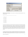
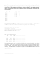
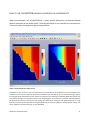
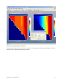
W2 VERSION 3.6 RELEASE NOTES
February 3, 2012
The code, updates and further information on the W2 model are available from the following web
page (subject to change):
http://www.ce.pdx.edu/w2
Please address questions about the code to
Scott Wells, Department of Civil and Environmental Engineering, Portland State University, P. O.
Box 751, Portland, OR 97207-0751, (503) 725-4276 FAX (503) 725-5950, e-mail:
[email protected]
Table of Contents
W2 Version 3.6 Release Notes ........................................................................................................................................... 1
W2 V3.6 Release Package ................................................................................................................................................... 2
How to use the Water balance Utility ................................................................................................................................ 4
How to use the MATFOR graphical interface on a windows PC ....................................................................................... 11
W2 Model Assistance for GUI Interface ........................................................................................................................... 13
W2 Known Issues .............................................................................................................................................................. 14
Internal weirs ................................................................................................................................................................ 15
Multiple dams into one downstream reach ................................................................................................................. 15
Problems reading file in GUI ......................................................................................................................................... 15
W2 V3.6 Bug Fixes, Enhancements, and User Manual Changes ...................................................................................... 16
W2 Planned Enhancements.............................................................................................................................................. 30
Differences between Version 3.6 and Version 3.5 ........................................................................................................... 30
Differences between Version 3.2 and Version 3.5 ........................................................................................................... 32
Differences between Version 3.1 and Version 3.2 ........................................................................................................... 43
W2 Version 3.6 Release Notes
1
W2 V3.6 RELEASE PACKAGE
The current release of the model includes the following:
1. The w2 model and preprocessor executables, source codes, and an example application
The model source code is found in 2 files: w2_IVF_source.zip and w2_generic_source.zip. The w2
executable is in w2_ivf.zip. The preprocessor source code and executable is in v36_
preprocessor.zip. The executables (prew2_ivf.exe and w2_ivf.exe) were compiled using Intel
Fortran 11 and are for 32-bit and 64-bit Windows computers. These executables need to be run in
the same directory as the input files (*.npt), unless the control file specifies file locations in other
directories. Also, generic FORTRAN source codes are included that the user can compile with
his/her FORTRAN 90/95 compiler on another platform.
Compiler settings for the Intel Visual Fortran compiler that were used for the w2_ivf.exe ‘release’
executables are:
/nologo /O3 /Og /Qparallel /real_size:64 /module:"Release\\" /object:"Release\\" /libs:static
/threads /winapp /c /Qopenmp-link:static
For WATER-QUALITY.F90, WQCONSTITUENTS.F90, and TRANSPORT.F90 the options were:
/nologo /Og /Qparallel /Qopenmp /real_size:64 /module:"Release\\" /object:"Release\\"
/libs:static /threads /winapp /c /Qopenmp-link:static
Included in this package is another set of files in the zip file: w2v36matfor.zip. This is an
executable and DLL files that include a PC animator that runs graphs up to 4 at a time based on
input from the file graph.npt and is only for Win32 bit environments at this time. This package
allows users to view during the model run a specified model state variable or derived variable and
to record that movie as an AVI file for later use. See the notes included below on how to use this
interface.
2. The GUI preprocessor
The GUI preprocessor is found in the file “gui.zip”. There is a “setup.exe” routine that installs the
Visual Basic W2 V3.6 Model Preprocessor called W2CONTROL. Once installed, the GUI
preprocessor is able to aid the model user in setting up the Control File and in evaluating and
W2 Version 3.6 Release Notes
2
changing the bathymetry of the system. This preprocessor does not automatically set-up the
bathymetry of the system, nor does it provide post-processing support. A lot of effort is required
to properly set-up the model bathymetry prior to using the Bathymetry editor within W2Control.
Also, note that on the W2 web page there may be updates to the file “w2control.exe”. If there are,
copy this new file over the one installed during the setup program. There is no need to run the
setup program again. Note that there is now a separate pdf user manual for the GUI interface. The
exe file, w2control, may work without going through the setup routine if you have Windows XP.
3. User’s Manual
On the web page the User’s Manual is provided in a zipped PDF file.
4. Waterbalance Utility
The code and executable for this are in the file “waterbalance.zip”. The purpose of this code is to
approximate the waterbalance for a reservoir by computing flows (positive and negative) that will
allow the model predicted water level to agree to water level data for a reservoir. See the notes
included below on how to use this interface. The code has been developed for a PC.
Registration information will be required for model download in order to alert users to bug fixes
and enhancements.
W2 Version 3.6 Release Notes
3
HOW TO USE THE WATER BALANCE UTILITY
RUNNING THE WATER BALANCE PROGRAM
When the executable is run, a window appears that allows the following inputs (note that the executable
runs under the Windows operating system only):
:
When the dialog box first appears, default values populate the edit boxes. The user can then edit
each one if the default values are not correct. Selecting Run will run the waterbalance utility to
completion as show in the following dialog box.
W2 Version 3.6 Release Notes
4
Observed elevations filename. This file consists of a Julian day and observed elevation as in the
following example:
2000-2001 Oologah Reservoir observed water surface elevations
JDAY
90.792
90.833
90.875
90.917
90.958
91.000
91.042
91.083
91.125
91.167
91.208
91.250
91.292
ELO
195.453
195.456
195.459
195.441
195.444
195.450
195.441
195.441
195.447
195.441
195.444
195.438
195.432
This example is prepared similar to all other CE-QUAL-W2 time-varying inputs with a fixed format with eight
columns each for the JDAY and ELO values. However, the utility will read in values using variable field
lengths so long as the JDAY and ELO values are separated by a space. Data need not be at regular intervals
that might cause a repeat of the same values. Better results will be obtained if the same values that repeat
over a time interval are not included. Doing this compresses the time interval that the utility uses to
compute the flows thus generating much larger flows over a shorter time interval, which is generally not
desirable.
For example, the water surface elevation at day 91.083 should be deleted in the above example. Also note
that the degree of accuracy in the observed elevations can have an impact on the computed flows. The
above example will yield different water balance flows if the elevations are rounded off to two decimal
W2 Version 3.6 Release Notes
5
places. If flows are computed at three and two decimal places for each date, the resulting files will have the
following positive/negative flows at the given time intervals if repeating elevations are eliminated,
assuming that the observed water surface elevation is constant at 195.453 m and 195.45, respectively,
over the time period. It is up to the user to decide the necessary precision used in the observed water
surface elevations.
JDAY
90.792
90.833
90.875
90.917
90.958
91.000
91.042
91.125
91.167
91.208
91.250
91.292
QWB
+
+
+
+
+
+
+
-
JDAY
90.792
90.958
91.000
91.083
91.125
91.292
QWB
+
+
-
Computed elevations filename. The following shows an example output file (the ……. leader indicates
that additional information is included in the time series output file, but is not included here):
Density placed inflow, point sink outflow
Default hydraulic coefficients
Default light absorption/extinction coefficients
Temperature simulation - run 29 turned WQ on
Tom Cole and Dottie Tillman - WES
Model run at 13:11:22 on 08/22/03
JDAY
DLT
ELWS..............................
92.000
456.39
195.37..............................
93.000
952.28
195.28..............................
94.000
494.28
195.27..............................
95.000
34.43
195.17..............................
96.000
170.88
195.08..............................
97.000
211.93
194.99..............................
98.000
255.11
194.92..............................
99.000
1459.08
194.78..............................
The water balance utility reads in the [JDAY] and [ELWS] values and uses these in the water balance
computations. The user must turn on time series output in the model control file and specify the segment
at which the water surface elevation values are output (typically the segment next to the dam for
reservoirs). Information on how to accomplish this is given in the User’s Manual under the Time Series
output file discussion.
W2 Version 3.6 Release Notes
6
Add to previous water balance. For various reasons, the water balance utility may not perfectly close
the water balance the first time through the computations. Depending upon the discrepancies between
computed and observed elevations, the utility may need to be used iteratively by rerunning the model
using output from the first run of the water balance utility and then rerunning the water balance utility on
the water surface elevations output in the new time series file. For a system with multiple branches, each
iteration of the utility and the resulting output file can be saved as a separate file that is then incorporated
as a distributed tributary for branch 2, then branch 3, etc. In the case of a system with only one branch,
this approach cannot be used. Rather, the new flows generated at the second iteration need to be added
to the previously computed flows and incorporated as an “improved” distributed tributary inflow file. This
option allows the user to continue adding flows to the same inflow file.
The computed flows are contained in the “qwb.opt” file. For most simulations, these flows will generate
water surface elevations sufficiently close to the observed elevations such that further refinement is
unnecessary. However, as mentioned above, the solution may need to be iterated. Rarely, manual
adjustment of the generated flows may be required. This is usually only needed when observed water
surface elevations change significantly over a short time period.
Previous water balance filename. If the “Add to previous water balance” option is used, you must
specify the existing water balance output file for the computed flows to be added to
Skip interval. Some reservoirs have a lot of noise in the observed water surface elevation data, such as in
peaking hydropower operations, and this option allows the user to specify how many observed elevations
are ignored when computing the flows between observed elevations. For example, if water surface
elevations are available on an hourly interval, the resulting flows generated by the water balance utility can
have large + and – flows that are completely unrealistic as opposed to using observed elevations on a daily
basis taken during periods of no hydropower generation. In order to smooth out the computed flows, a
skip factor of 24 would result in computed flows being output on a daily basis with all of the “noise”
generated by hydropower operations ignored over the 24 hour period.
Averaging interval. This option computes a running average of the water surface elevation based on the
input value. This is an additional aid to smooth out water surface elevation “noise”. For example, consider
the case in which there is no inflow/outflow to the system, but there is considerable wind seiching. The
water balance utility would compute alternating inflows and outflows from the system that, depending on
the amount of seiching, could be very large when in reality there should not be any flows added to or
subtracted from the system. Using a running average alone or in combination with skipping over a number
of observed elevations specified in (4) can help alleviate many of the problems caused by an automated
water balance computation.
W2 Version 3.6 Release Notes
7
Waterbody number. In the case of multiple waterbodies each of which has a separate bathymetry input
file, the user must specify which waterbody (and thus which bathymetry file) the water balance is being
computed for. This capability is necessary for modeling systems with multiple reservoirs.
INCORPORATING THE COMPUTED FLOWS INTO THE SIMULATION
The water balance utility can be used for lakes and reservoirs in which water surface elevations are a
function of inflows and controlled outflows from the system. The utility computes the flows necessary to
match observed water surface elevations (typically taken at the dam) and outputs them to the “qwb.opt”
file. This file is composed of a Julian date and an inflow (m3 sec-1). The flows can be either positive or
negative. Temperatures and/or constituent concentrations must also be provided in the corresponding
temperature and constituent concentration input files if the computed flows are incorporated as inflows to
the system. The water balance utility does not provide this information, but this information needs to be
provided by the user depending upon how the computed flows are incorporated into the simulation.
Considerable thought should go into how best to incorporate temperature and constituent concentrations
and is discussed in more detail below.
Note that negative flows use temperatures/concentrations in the waterbody when calculating the impact
on the system of these flows rather than the temperatures/concentrations in the corresponding inflow
temperature and constituent concentration files. This ensures that negative flows generate no change in
temperature or constituent concentrations. However, positive flows can impact simulation results and care
must be taken as to how the flows are incorporated into the simulation.
The flows required to complete the water balance are computed as a step function. If they are
incorporated into the model as an additional inflow or outflow whose current values are being linearly
interpolated, such as a branch inflow, then the resulting water balance will not be correct. Typically, the
flows in the qwb.opt file are first included as a distributed tributary inflow assigned to the mainstem branch
and interpolation [DTRIC] is turned “OFF”. The corresponding distributed tributary inflow temperatures are
usually set to air temperatures in the qdt_br1.npt file. When running water quality, care must be taken as
to what constituents should be included in the corresponding inflow constituent concentration file.
Typically, only DO values are included if the distributed tributary option of incorporation is used, and they
are set to saturated values corresponding to the observed air temperatures. Keep in mind that if the water
balance flows are incorporated as branch inflows, then the mass loading of organic matter and nutrients
will be increased as well.
W2 Version 3.6 Release Notes
8
The branch corresponding to the distributed tributary inflow is usually assigned to the mainstem branch of
a reservoir. Using a distributed tributary minimizes the impact of the flow, temperature, and/or water
quality associated with the distributed tributary by distributing the flow throughout all segments in a
branch weighted by surface area. Be aware that large flows as a result of large errors in inflow/outflow
measurements can and have had a significant impact on temperature and water quality calibration in the
surface layers. Usually, this is not a problem, but sensitivity analyses should be conducted to see if the flow
and associated temperature/constituent concentrations have an impact on the simulation results. If so,
then the following discussion is of particular relevance.
As emphasized previously, a great deal of thought should go into how the flows generated from the water
balance utility are incorporated into the simulation. As discussed previously, these are typically
incorporated as distributed tributary inflows so as to minimize the impact of the flows on the simulation.
However, this may not always be the best, most accurate, or most realistic method. For example, suppose
that the water balance flows are consistently negative. This would indicate that either inflows are
consistently overestimated or outflows are consistently underestimated. Obviously, incorporating the
flows as a positive increase in the outflows as opposed to subtracting them from the inflows can potentially
have a very significant impact on simulation results. In this case, sensitivity analyses should be conducted
to determine which method improves the simulation results. If, say, hypolimnetic temperatures are
consistently being underestimated, then incorporating the flows into a hypolimnetic outflow could improve
the simulation results. Conversely, if hypolimnetic temperatures were being overpredicted, then the
inflows should probably be reduced. The key point to keep in mind is that there are a number of different
ways to incorporate the computed flows, and they generally should all be tested to determine the best way
to incorporate the computed flows into the simulation.
As another example, consider the case in which the generated flows are consistently positive and a branch
in which sometimes significant inflows are ungauged. In this case, a sensitivity analyses should be
performed to determine if incorporating the flows or a portion of the flows into the ungauged branch
inflow improves model results. Oftentimes, the model can be used as a guide as to how best to incorporate
the computed flows into the simulation.
REAL WORLD EXAMPLE
Walter F. George is a U.S. Army Corps of Engineer reservoir located on the Chattahoochee River in
Alabama. The reservoir is operated as a peaking hydropower facility. During calibration, the model
consistently underpredicted hypolimnetic temperatures by 0.5-1ºC. Wind sheltering could be adjusted to
increase hypolimnetic temperatures, but this adjustment always adversely impacted thermocline depth.
After considerable thought, it was concluded that including possible seepage at the dam might improve
W2 Version 3.6 Release Notes
9
hypolimnetic temperature predictions. A portion of the distributed tributary flows were incorporated as an
additional outflow at the bottom of the dam. The final value used was 5 m3 sec-1, which was less than 1% of
the average outflows, and brought hypolimnetic temperatures into almost exact agreement with observed
temperatures. Further investigation of the outflows revealed that during times of no power generation, an
additional flow of 5.1 m3 sec-1 was specified in a file that was not originally sent as part of the outflow data.
Thus, the model pointed the way as to how best to incorporate the computed flows and was a surprisingly
accurate indicator of what was actually occurring in the prototype.
W2 Version 3.6 Release Notes
10
HOW TO USE THE MATFOR GRAPHICAL INTERFACE ON A WINDOWS PC
When the executable “w2_ivf_MATFOR.exe” is used, another dialog box is presented showing
dynamic animation of the model results. The dialog box below is one example of an animation for
a reservoir system showing water age and temperature.
FIGURE 1. MATFOR ANIMATION OF MODEL RESULTS.
The model DLL files must be in the same directory as the executable for this animation to work. The details of the
animation are set out in the graph.npt file which is described in the User Manual. For this animation though, only the
first 4 graphs will be animated. If the user presses the red button for recording, the following dialog box asks the user
to record the animation as an AVI file as shown in the following figure. The model user must enter a filename with the
AVI file suffix to produce an AVI file for later viewing. Be careful when setting the SCR update frequency to a high
frequency since the file size of the AVI file can grow significantly such that your AVI file is too big for later viewing. This
can be adjusted in the control file (w2_con.npt SCR FREQ).
W2 Version 3.6 Release Notes
11
FIGURE 2 DIALOG BOX FOR RECORDING THE ANIMATION.
The “pause” button allows the user to pause the animation so that a graph can be printed. By pausing the animation,
the model stops running until the play button is pushed.
W2 Version 3.6 Release Notes
12
W2 MODEL ASSISTANCE FOR GUI INTERFACE
The following list provides information to assist the model user to set up the program and files.
#
Item
Description
2
GUI Interface
Install this using the setup.exe file. Also, if there is a newer w2control.exe file in
the zip file on the FTP site than installed during setup, use this latest
w2control.exe file by overwriting the one installed during setup. The latest file
includes the latest bug fixes.
W2 Version 3.6 Release Notes
13
W2 KNOWN ISSUES
The following list shows known bugs and issues with the current release of the code - these are
being addressed in the next release:
#
Item
Description
1
Water levels
"bowl"
2
Pipes under high head
The pipes algorithm does not handle high-head, dynamic flow conditions in a
pipe.
3
Time step limitation in
a complex system
model
The time step for stability in a system model is governed by the lowest time
step for numerical stability. If you have a very dynamic river with several
reservoirs, the time step for the river will control. This can result in very long
run times. One can still break apart the model and run the pieces separately
using the WDOUT files to provide boundary conditions for downstream
waterbodies.
4
Partitioning
The partitioning coefficient is currently constant for all organic and inorganic
compartments
5
Internal weir at a Dam
segment
Putting an internal weir at a Dam segment does not affect the outflow from
the selective withdrawal structure. One must limit selective withdrawal rather
than use an internal weir at the dam segment. Remember the internal weir
works for the right-hand-face of a model layer.
6
W2 multiple file error
check
If the model user accidentally enters duplicate file names for an input file, the
w2 executable will "bomb" because it will try to read the file in more than
once. The first use of the file will lock its availability for the second instance.
The W2 error message that comes on the screen (traceback error) should
mention the file name that has problems. The W2 preprocessor should catch
this potential error.
7
Raising
level
of
spillway/weir
above
grid
The preprocessor will say there is an error if the user raises the weir, spillway,
gate, water level control or any other hydraulic element above the current
top-of-the-grid. The w2 code will still run properly though. But more correctly,
the model user should increase the DZ of the upper-most layer to a value that
would eliminate this problem. But keep in mind that the segment widths from
the top layer then extend upward at that same width.
in
W2 Version 3.6 Release Notes
a
If water levels decrease in a waterbody shaped like a "bowl", the removal of
model layers as the water level decreases will cause the model to bomb if an
upstream segment dries up.
14
#
8
9
Item
Description
INTERNAL WEIRS
The internal weir algorithm does not work when all vertical layers of a
segment are blocked by the weir.
MULTIPLE DAMS INTO
ONE DOWNSTREAM REACH
10
11
PROBLEMS READING FILE
IN GUI
RESTART FROM RUN
WINDOW
W2 Version 3.6 Release Notes
Currently, the code will allow one dam inflow to a downstream branch by a
user-specified outflow file. The code though does allow multiple dams
inflowing to a common downstream branch if the outflow is specified as a
hydraulic structure.
Sometimes the control file or bathymetry file cannot be read properly by the
GUI interface. This can be a result of the text editor used to produce the file.
[You will find that the problem file(s) look all messed up in NOTEPAD but look
OK in the PFE Editor or in WORD; and W2 usually can read them OK.]
Sometimes the following will “fix” the formatting:
(1)
Copy the file to a UNIX workstation and copy it back.
(2)
Load the file in WORD as a Text file, add a space somewhere in the
file (but don’t mess up the file formatting), then save it as a Text
file.
(3)
Convert all tabs to ‘spaces’
When using the MATFOR visualization, stopping a simulation and then
pressing the RESTART button results in the code exiting with an error
message. This is being worked on. The RESTART capability within the control
file works fine.
15
W2 V3.6 BUG FIXES, ENHANCEMENTS, AND USER MANUAL CHANGES
#
Code: W2
or PREW2
or GUI
Fix
or
Enhancement
Type
Description of Bug/Enhancement
Date
Bug
Fixed
or
Enhancemen
t added
1
W2
TKE1 model
The variable STRICK was incorrectly allocated as
an INTEGER rather than REAL.
10/11/2008
2
W2
PIPE
Code was streamlined in the subroutine ZBRENT
where calls were made directly to CDFUNC
rather than through the dummy function FUNC
10/11/2008
3
W2 Manual
Z0
The User Manual had Z0 in an incorrect line in
the control file (w2_con.npt). The write up and
example control file in the User Manual were
corrected.
10/28/2008
4
W2
Longitudinal
profile input
The W2 program did not read initial constituent
concentrations in the longitudinal profile file
when CCC was 'OFF'. This has been fixed.
12/4/2008
5
W2
TECPLOT
output
When using TECPLOT output for multiple
waterbodies, the output format did not allow
loading the information into TECPLOT. Fixed.
1/26/2009
6
W2
Epiphyton
input
5/21/2009
7
PreW2
Constituent
loads
For entering vertical profile data for periphyton, there was an
index error:
OLD CODE:
IF (VERT_EPIPHYTON(JW,JE)) EPD(:,I,JE) = EPIVP(K,JW,JE)
NEW CODE:
IF (VERT_EPIPHYTON(JW,JE)) EPD(:,I,JE) = EPIVP(:,JW,JE)
An enhancement was added to the Preprocessor to compute
loads in kg/day for all inflow, tributary and distributed
tributaries. Also, these are summed up for the model
application. These are shown in the file “pre.opt”. These are
approximate loads since the concentration data are used to
set the frequency of loading update. Flow rates at the time of
the concentration input data are used to compute load.
W2 Version 3.6 Release Notes
5/21/2009
16
#
Code: W2
or PREW2
or GUI
Fix
or
Enhancement
Type
Description of Bug/Enhancement
Date
Bug
Fixed
or
Enhancemen
t added
8
W2
Gas transfer
at spillways
A couple code fixes in the hydroinout.f90 subroutine:
(1) CGAS needed to be initialized in some cases to
CGAS=C2(K,ID,CN(JC)) prior to calling the
subroutine TOTAL_DISSOLVED_GAS
for use in the Butts and Evans (1983) equation:
NEW CODE:
CGAS=C2(K,ID,CN(JC)) ! MM 5/21/2009
5/21/2009
(2)
9
W2
Reaeration
from dams
W2 Version 3.6 Release Notes
Change logic in several lines from
IF(CAC(NDO) == ‘ ON’ to
IF(CAC(NDO) == ‘ ON’ .and. CN(JC)==NDO
NEW CODE:
IF (CN(JC)==NDO .AND. CAC(NDO) ==
'
ON' .AND. GASSPC(JS) == '
ON'
.AND. QSP(JS) > 0.0) THEN
! MM 5/21/2009
An error was found in the formulae from Butts and Evans
(1983).
OLD CODE:
DB = SAT-C
DA =
DB*(1.0+0.38*AGASGT(N)*BGASGT(N)*CGASGT(N
)*(1.0-0.11*CGASGT(N))*(1.0+0.046*T))
C = SAT-DA
NEW CODE:
DA = SAT-C
! MM 5/21/2009 DA: Deficit upstream
DB =
DA/(1.0+0.38*AGASSP(N)*BGASSP(N)*CGASSP(N
)*(1.0-0.11*CGASSP(N))*(1.0+0.046*T))
! DB: deficit downstream
C = SAT-DB
5/21/2009
17
#
Code: W2
or PREW2
or GUI
Fix
or
Enhancement
Type
Description of Bug/Enhancement
Date
Bug
Fixed
or
Enhancemen
t added
10
W2
Order of flux
parameters
The order of flux parameters in the User
Manual and output were incorrect. The
control file has them in this order:
RPOMSET
CBODDK
DOAP
DOAR
DOEP
DOER
DOPOM
DODOM
DOOM
6/2/2009
whereas the code assumed they were in
this order:
RPOMSET
CBODDK
DOAP
DOEP
DOAR
DOER
DOPOM
DODOM
DOOM
This has been corrected. The User Manual
and control file order is now reflected
in the W2 code.
11
Pre
False errors
for
inflow
location
The preprocessor sometimes gave false errors in the
pre.err for tributary, internal weirs, pipes, and other
hydraulic features saying that the pipe or tributary
was below the elevation of the bottom of the
segment. The W2 model ran fine even with this error
message given in the preprocessor. This has been
fixed.
6/18/09
Example of OLD CODE:
IF (EBTR(JT) <
EL(KB(ITR(JT)+1),ITR(JT))) THEN
CALL ERRORS
WRITE
(ERR,FMTFI)
'Inflow
placement
bottom
elevation
[EBTR=',EBTR(JT),'] < bottom active cell
elevation for tributary ',JT
New CODE:
IF (EBTR(JT) <
EL(KB(ITR(JT))+1,ITR(JT))) THEN
CALL ERRORS
WRITE
(ERR,FMTFI)
'Inflow
placement
bottom
elevation
[EBTR=',EBTR(JT),'] < bottom active cell
elevation for tributary ',JT
W2 Version 3.6 Release Notes
18
#
Code: W2
or PREW2
or GUI
Fix
or
Enhancement
Type
Description of Bug/Enhancement
Date
Bug
Fixed
or
Enhancemen
t added
12
Pre
Additional
error checking
6/22/09
13
Pre
Command line
processing
and working
directory
displayed for
windows
Additional error checking was added to help debug an
error in the bathymetry file when the problem was in
the branch connectivity specifically BS and BE. Also, a
false error was given when the temperature had an
isothermal initial condition, constituents were OFF,
and an initial concentration was set to “-2”. This was
fixed.
In the windows version of the preprocessor, the user
can now supply a command line argument that sets
the working directory of the code. Hence, one does
not need to copy the preprocessor into every
directory. In a batch file, for example, one can execute
the following command:
9/12/09
preW2_ivf.exe "C:\scott\w2workshop\2009
workshop\waterqual\problem3"
The preprocessor now uses the supplied directory (in
double quotes) as the working directory for all the
files. The command line argument has one blank space
between the end of the executable and the first
quote. Also, the working directory is now displayed at
the top of the window.
14
W2
#
of
processors
W2 Version 3.6 Release Notes
Additional checks were also added for checking the
grid linkage.
The model user can now control the # of physical
processors the model uses. At this point, dualprocessor model runs have shown an improvement of
about 20% over a single processor. But, QUAD
processors usually are slower. It is recommended that
NPROC be set to 2 in the control file. The user can
experiment on his/her own system. If this is not set by
the user or is left blank, the model still runs but sets it
to 2 processors.
GRID
NPROC
CLOSEC
2
ON
NWB
NBR
IMX
KMX
1
1
23
22
9/12/09
19
#
Code: W2
or PREW2
or GUI
Fix
or
Enhancement
Type
Description of Bug/Enhancement
Date
Bug
Fixed
or
Enhancemen
t added
15
W2
Command line
processing for
windows
In the windows version of the w2 model, the user can
now supply a command line argument that sets the
working directory of the code. Hence, one does not
need to copy the model executable into every
directory. In a batch file, for example, one can execute
the following command:
9/12/09
W2_ivf.exe "C:\scott\w2workshop\2009
workshop\waterqual\problem3"
16
W2
W2 window
closed at end
of successful
execution
The w2 model now uses the supplied directory (in
double quotes) as the working directory for all the
files. The command line argument has one blank space
between the end of the executable and the first
quote. The working directory is displayed in a text box
in the window.
At the end of a windows run, the windows dialog box
waits for the user to press ‘close’ to exit the window.
This allows the user to examine the final run
parameters. In the w2_con.npt file there is now an
option to close this window when the run has
completed. If this option is not set, then the dialog box
will stay until the user clicks ‘close’.
9/12/09
This allows for efficient batch processing of the model,
especially if user in conjunction with command line
processing mentioned in #15.
17
User
Manual
Updates
W2 Version 3.6 Release Notes
GRID
NPROC
CLOSEC
0
ON
NWB
NBR
IMX
KMX
1
1
23
22
When CLOSEC is set to ON, then the dialog box will
disappear once the run finishes. If it is set to OFF, then
the dialog box will remain until the user clicks ‘close’.
Updates and changes to the control file (#13-#16)
were reflected in an updated User Manual.
9/12/09
20
#
Code: W2
or PREW2
or GUI
Fix
or
Enhancement
Type
Description of Bug/Enhancement
Date
Bug
Fixed
or
Enhancemen
t added
18
GUI
Updates
The GUI was updated with the following:
(1) new control file parameters NPROC and
CLOSEC were added (see #14 and 16). There
is also a SELECTC that will be used in V3.7
that has been included – ignore it for now.
(2) The GUI also can be controlled by command
line passing of the working directory and file.
In a batch program or from the command
line in a DOS box you can execute the GUI as
follows:
9/12/09
"C:\scott\research\corps of
engineers\tomcole\w2code\GUI36\w2control\
w2control36.exe" C:\scott\w2workshop\2009
workshop\waterqual\problem1\w2_con.npt
The first string in quotes executes the GUI. The
command line argument is NOT in quotes. This
program was developed in VB6 and does not take
quotes around the command line. Note that this is
different than the FORTRAN command line argument.
So the above command will open the GUI and load the
control file automatically.
(3) A text box now shows the file path and
name of the file that you are working on
(4) In file open, earlier all *.npt files were
shown. Since only “w2_con.npt” files are
loaded into the GUI, only the “w2_con.npt”
file was shown for opening.
W2 Version 3.6 Release Notes
21
#
Code: W2
or PREW2
or GUI
Fix
or
Enhancement
Type
Description of Bug/Enhancement
Date
Bug
Fixed
or
Enhancemen
t added
19
W2
Gates,
spillways,
pipes
Whenever DOWN was specified for a gate, spillway or
pump, the model estimated the water level at the end
of the segment, rather than using the branch center
water level. This is important in sloping river systems
where a long segment may have a water surface
elevation drop between the segment center and the
edge. In the past this was computed assuming the
slope of the channel. This was updated to estimate the
water surface elevation using linear interpolation
rather than the grid slope. Below is an example of the
code fix – in this case for GATES:
9/25/09
OLD CODE:
ELIU=ELWS(IUGT(JG))SINA(JBUGT(JG))*DLX(IUGT(JG))*0.5
NEW CODE:
ELIU= ELWS(IUGT(JG)) + (ELWS(IUGT(JG))ELWS(IUGT(JG)1))/(0.5*(DLX(IUGT(JG))+DLX(IUGT(JG)1)))*DLX(IUGT(JG))*0.5
20
W2
New
executable
W2 Version 3.6 Release Notes
A new executable was made using a new release of
Intel Version 11 compiler that corrected problems
with Windows 7 applications.
9/25/09
22
#
Code: W2
or PREW2
or GUI
Fix
or
Enhancement
Type
Description of Bug/Enhancement
Date
Bug
Fixed
or
Enhancemen
t added
21
W2
ICE
cover
algorithm
There were a couple logic errors in the ice cover
algorithm. These were corrected below:
10/20/09
!************** Ice thickness
ICETH(I) =
ICETH(I)+ICETHU+ICETH1+ICETH2
IF (ICETH(I) < ICE_TOL)
ICETH(I) = 0.0
IF (WINTER .AND. (.NOT.
ICE_IN(JB))) THEN
IF (.NOT. ALLOW_ICE(I))
ICETH(I) = 0.0
END IF
ICE(I)
= ICETH(I) > 0.0
IF (ICE(I))THEN
!
3/27/08 SW
ICESW(I) = 0.0
ELSE
ICESW(I) = 1.0
ENDIF
ICETHU
= 0.0
ICETH1
= 0.0
ICETH2
= 0.0
IF (ICETH(I) < ICE_TOL
.AND. ICETH(I) > 0.0) ICETH(I) = ICE_TOL
ELSE
IF(TERM_BY_TERM(JW))CALL
EQUILIBRIUM_TEMPERATURE
! SW
10/20/09 Must call this first otherwise
ET and CSHE are 0
HIA
=
0.2367*CSHE(I)/5.65E-8
! JM 11/08 convert SI units of m/s to
English (btu/ft2/d/F) and then back to SI
W/m2/C
!
ICETH(I) =
MAX(0.0,ICETH(I)+DLT*((RIMTET(I))/(ICETH(I)/RK1+1.0/HIA)-(T2(KT,I)RIMT))/RHOIRL1)
! OLD CODE
ICETH(I) =
MAX(0.0,ICETH(I)+DLT*((RIMTET(I))/(ICETH(I)/RK1+1.0/HIA)HWI(JW)*(T2(KT,I)-RIMT))/RHOIRL1)
! SW
10/20/09 Revised missing HWI(JW)
ICE(I)
= ICETH(I) > 0.0
ICESW(I) = 1.0
IF (ICE(I)) THEN
!
TFLUX
= 2.392E7*(RIMT-T2(KT,I))*BI(KT,I)*DLX(I) ! OLD
CODE
TFLUX
= 2.392E7*HWI(JW)*(RIMT-T2(KT,I))*BI(KT,I)*DLX(I)
! SW 10/20/09 Revised missing HWI(JW)
TSS(KT,I) = TSS(KT,I)
+TFLUX
TSSICE(JB) =
TSSICE(JB)+TFLUX*DLT
ICESW(I) = 0.0
END IF
END IF
END DO
END IF
END IF
W2 Version 3.6 Release Notes
23
#
Code: W2
or PREW2
or GUI
Fix
or
Enhancement
Type
Description of Bug/Enhancement
Date
Bug
Fixed
or
Enhancemen
t added
22
W2
Gates output
in QWD file
The following bug was found in defining which branch
a gate was located. This affected the output for the
withdrawals at a location where there were gates that
were not tied to other branches.
3/24/10
Old code:
JWUGT(JG) = JW
IF (IDGT(JG) > 0) THEN
DO JB=1,NBR
IF (IDGT(JG) >= US(JB) .AND.
IDGT(JG) <= DS(JB)) EXIT
END DO
JBDGT(JG) = JB
DO JW=1,NWB
IF (JB >= BS(JW) .AND. JB <=
BE(JW)) EXIT
END DO
JWDGT(JG) = JW
else ! BUG FIX 9/27/07
jbdgt(jp)=1
jwdgt(jp)=1
END IF
New code:
JWUGT(JG) = JW
IF (IDGT(JG) > 0) THEN
DO JB=1,NBR
IF (IDGT(JG) >= US(JB) .AND.
IDGT(JG) <= DS(JB)) EXIT
END DO
JBDGT(JG) = JB
DO JW=1,NWB
IF (JB >= BS(JW) .AND. JB <=
BE(JW)) EXIT
END DO
JWDGT(JG) = JW
else ! BUG FIX 9/27/07
jbdgt(jg)=1
! SW 3/24/10
jwdgt(jg)=1
! SW 3/24/10
END IF
W2 Version 3.6 Release Notes
24
#
Code: W2
or PREW2
or GUI
Fix
or
Enhancement
Type
Description of Bug/Enhancement
Date
Bug
Fixed
or
Enhancemen
t added
23
PreW2
Reading
WSC
Reading in of the WSC file was limited to only 100
dates in the preprocessor. This limitation was fixed by
the code shown below:
3/26/10
of
!
DO J=1,100
28995 continue ! cb 3/26/10
READ
(NPT,'(10F8.0:/(8X,9F8.0))',END=29000)
SDAY,(WSC(I),I=1,IMX)
IF (SDAY <= SDAYO) THEN
CALL ERRORS
WRITE (ERR,'(3(A,F0.3))')
'Julian date ',SDAY,' <= previous date of
',SDAYO,' in '//WSCFN
END IF
DO I=1,IMX
IF(WSC(I) <= 0.0)THEN
CALL ERRORS
WRITE (ERR,'(A,F0.3,A,I4,A)')
'Julian date ',SDAY,': WSC AT
SEG(I)=',I,' <= 0.0 in '//WSCFN
ENDIF
IF (WSC(I) > 2.0) THEN
CALL WARNINGS
WRITE (WRN,'(A,F0.3,A,I4,A)')
'Julian day ',SDAY,': WSC(I) AT
SEG(I)=',I,' > 2.0 in '//WSCFN
END IF
IF (WSC(I) > 0.0 .and. wsc(i) <
0.5) THEN
CALL WARNINGS
WRITE (WRN,'(A,F0.3,A,I4,A)')
'Julian day ',SDAY,': WSC(I) AT
SEG(I)=',I,' < 0.5 in '//WSCFN
END IF
ENDDO
SDAYO=SDAY
! ENDDO
go to 28995
24
PreW2
Check on LAT
or DOWN
25
W2 Manual
Light
extinction, ice
26
W2 Manual
Precipitation
input file
W2 Version 3.6 Release Notes
! cb 3/26/10
Added an enhancement to do a check in case a
spillway, pipe, pump, or gate was specified as ‘DOWN’.
In all cases where ‘DOWN’ is specified, the segment
that the hydraulic structure originates must be at the
end of a branch. Additional logic was added to check
for this in all the hydraulic structures.
Added more text to the section on computation of
light extinction and inserted a missing reference.
Revised an equation for clarity in ICE algorithm and
added more explanation on how to estimate HICE.
The units of precipitation are in m/s. The example
precipitation input file was changed to more realistic
values.
3/26/10
4/13/2010
4/14/2010
25
#
Code: W2
or PREW2
or GUI
Fix
or
Enhancement
Type
Description of Bug/Enhancement
Date
Bug
Fixed
or
Enhancemen
t added
27
W2
ICE
Added code to account for the need to compute long
wave radiation in case user chose the equilibrium
temperature approach. Fixed subscript error in ice
melt computation. Also, made the variable TICE
double precision since it is assumed double precision
in the call to Surface_terms.
4/19/10
New code:
IF (ICE(I)) THEN
TICE = TAIR(JW)
DEL = 2.0
J
= 1
if(tair(jw).ge.5.0)then ! SW 4/19/10
RANLW(JW) = 5.31E13*(273.15+TAIR(JW))**6*(1.0+0.0017*CLOUD
(JW)**2)*0.97
else
RANLW(JW) = 5.62E8*(273.15+TAIR(JW))**4*(1.-0.261*exp(7.77E4*TAIR(JW)**2))*(1.0+0.0017*CLOUD(JW)**2)
*0.97
endif
RN1=SRON(JW)/(REFL*RHOWCP)*SHADE(I)*(1.0ALBEDO(JW))*BETAI(JW)+RANLW(JW)
! SW 4/19/10
DO WHILE (DEL > 1.0
.AND. J < 500)
CALL SURFACE_TERMS
(TICE)
RN(I) = RN1-RB(I)RE(I)-RC(I)
! 4/19/10
!
RN(I) =
SRON(JW)/(REFL*RHOWCP)*SHADE(I)*(1.0ALBEDO(JW))*BETAI(JW)+RANLW(JW)-RB(I)RE(JW)-RC(I) ! OLD CODE
DEL
=
RN(I)+RK1*(RIMT-TICE)/ICETH(I)
IF (ABS(DEL) > 1.0)
TICE = TICE+DEL/500.0
J = J+1
END DO
28
W2
Evaporation
W2 Version 3.6 Release Notes
Units for EV in the SNP file were given in m/s but were
actually m^3/s
4/21/10
26
#
Code: W2
or PREW2
or GUI
Fix
or
Enhancement
Type
Description of Bug/Enhancement
Date
Bug
Fixed
or
Enhancemen
t added
29
W2
Ice
In the ice melt algorithm, SRON should not have been
divided by RHOCP in computing RN1 and DEL in the
DO WHILE loop should have been ABS(DEL) rather
than DEL:
4/21/2010
RN1=SRON(JW)/REFL*SHADE(I)*(1.0ALBEDO(JW))*BETAI(JW)+RANLW(JW)
! SW 4/19/10 eliminate spurious divsion
of SRO by RHOCP
DO WHILE (ABS(DEL) > 1.0 .AND. J <
500)
! SW 4/21/10 Should have been ABS of DEL
CALL SURFACE_TERMS (TICE)
30
PRE
Constituent
loading
The output from the preprocessor in the pre.opt file
for constituent loading was in kg rather than the
output header of kg/day. The output was updated to
kg/day by adding the following lines of code:
5/10/10
cdtload(incdt(1:NACdt(Jb),Jb),jb)=cdtload
(incdt(1:NACdt(Jb),Jb),jb)/(jday-tstart)
! CB 5/10/10 Change units to kg/day
ctrload(trcn(1:NACtr(Jt),Jt),jt)=ctrload(
trcn(1:NACtr(Jt),Jt),jt)/(JDAY-TSTART)
!CB 5/11/10 convert to units of kg/day
W2 Version 3.6 Release Notes
27
#
Code: W2
or PREW2
or GUI
Fix
or
Enhancement
Type
Description of Bug/Enhancement
Date
Bug
Fixed
or
Enhancemen
t added
31
W2
Gate,
spillways,
pipes
In the case where the user has specified that the flow
is DOWN, in the case of reverse flow, the model did
not assign the flow correctly if the user had no other
tributaries or withdrawals specified in the control file.
For this rare event, additional code was written to
account for this fact. Also, a logic error was discovered
in reverse flow for spillways and gates. This was
corrected.
6/4/10
New code added to hydroinout.f90:
JWW = NWD
withdrawals = jww > 0
JTT = NTR
tributaries = jtt > 0
JSS = NSTR
IF (SPILLWAY) THEN
! 6/4/10 SW
! 6/4/10 SW
…
END IF
tributaries = jtt > 0
withdrawals = jww > 0
! 6/4/10 SW
! 6/4/10 SW
DO JW=1,NWB
KT = KTWB(JW)
DO JB=BS(JW),BE(JW)
New code in gate-spill-pipe.f90:
For spillway:
IF (ISUB == 0) THEN
DLEL = ELIU-ESP(JS)
IF (ELID > ESP(JS)) DLEL = ELIU-ELID
! SW 6/7/10
IF (DLEL < 0.0) THEN
DLEL
= -DLEL
For gates:
IF (A2GT(JG) == 0.0 .AND. G2GT(JG) /= 0.0)
DLEL = ELIU-G2GT(JG)
IF (ELID > EGT(JG)) DLEL = ELIU-ELID
! SW 6/7/10
IF (DLEL < 0.0) THEN
W2 Version 3.6 Release Notes
28
#
Code: W2
or PREW2
or GUI
Fix
or
Enhancement
Type
Description of Bug/Enhancement
Date
Bug
Fixed
or
Enhancemen
t added
32
W2
Branch
intersections
with multiple
waterbodies
In cases where there are branch intersections
between waterbodies, it was possible that the variable
KBI and KB were incorrectly set. Here is the fix: Move
the statement defining KBI in the subroutine initgeom.f90 to the place shown below (delete the earlier
reference):
10/30/2010
IF (B(K,ID+1) == 0.0) B(K,ID+1) = B(K1,ID+1)
IF (IEXIT == 1) EXIT
END IF
END IF
END IF
END DO
END DO
! SW 1/23/06
END DO
! SW 1/23/06
bnew=b
! SW 1/23/06
KBI = KB ! SW 10/30/2010
!**** Upstream active segment and single
layer ! 1/23/06 entire section moved SW
DO JW=1,NWB
KT = KTWB(JW)
DO JB=BS(JW),BE(JW)
33
W2
SS
resuspension
The code index was incorrect in the loop for
computing resuspension. This led in some compilers to
an infinite loop.
The corrected code is shown below:
2/3/2012
SSSS(KT,I,J)
=
SSS(J)*SS(KT,I,J)*BI(KT,I)/BH2(KT,I)+SSR
! DO K=KT-1,KB(I)-1
DO
K=KT,KB(I)-1
! JP 2/3/12
IF (SEDIMENT_RESUSPENSION(J)) THEN
Thanks to James Pasley for this bug report/fix.
W2 Version 3.6 Release Notes
29
W2 PLANNED ENHANCEMENTS
The following list shows planned enhancements:
#
Item
Description
1
Sediment
Diagenesis
Complex sediment diagenesis model
2
Simultaneous
Currently, water surface is solved branch-by-branch.
water
level The new technique will involve solving all water
solution
surfaces for the system or waterbody simultaneously.
3
W3
4
Hypoheric
algorithm
5
Sediment channel Dynamic heat transfer between channel bottom and
bottom
heating stream
algorithm
3D version of W2
flow Groundwater-surface water interaction
DIFFERENCES BETWEEN VERSION 3.6 AND VERSION 3.5
Version 3.6 can be run without changing any of the input files, even though the preprocessor will identify errors in the
control file because of missing variables. Below is a highlighted list of locations in the file w2_con.npt where additional
variables have been added. There are no other changes in the input files for Version 3.6.
The TKE algorithm has been updated with new algorithms that match experimental tank data for kinetic energy and
dissipation. This is based on a Master’s degree project by Sam Gould at Portland State University. A new user option is
the TKE1 algorithm, in add addition to the legacy algorithm TKE. This results in several new input variables on the
following line of the w2_con.npt file that are only active if TKE1 is chosen for AZC:
EDDY VISC
WB 1
AZC
W2
AZSLC
AZMAX
IMP 1.00000
FBC
3
E
9.535
ARODI STRCKLR BOUNDFR
0.430
24.0
10.00
TKECAL
IMP
The roughness height of the water for correction of the vertical velocity wind profile is now a user-defined input, z0.
Prior to this the model had hardwired the value of z0=0.003 m for wind speed correction at 2m (for evaporation where
W2 Version 3.6 Release Notes
30
wind height at 2 m is typical) and z0=0.01 m for wind at 10 m (for shear stress calculations where wind height of 10 m
is typical). For consistency, both conversions now use the same value of roughness height. If the user does not specify
the value of z0 (for example if he/she leaves the spaces blank for z0 using a V3.5 control file), the code uses 0.001 m.
HYD COEF
AX
DX
CBHE
TSED
FI
TSEDF
WB 1
1.00000 1.00000 0.30000 11.5000 0.01000 1.00000
FRICC
MANN
Z0
0.001
A new option for output is in the format required for TECPLOT. For TECPLOT animation there is only a flag in the CPL
output line. This allows for easy model animation of the variables U, W, T, RHO, and all active constituents at the
frequency specified by the CPL file as a function of distance and elevation.
CPL PLOT
WB 1
CPLC
ON
NCPL TECPLOT
1
ON
A new variable for determining the fraction of NO3-N that is diffused into the sediments that becomes organic matter,
or SED-N was introduced. According to one study, only about 37% of NO3-N that diffuses into the sediments becomes
incorporated into organic matter in the sediments. The rest is denitrified.
NITRATE
Wb 1
Wb 2
NO3DK
0.05
0.05
NO3S FNO3SED
0.0
0.37
0.0
0.37
In V3.5 the model computed an average decay coefficient of the sediments based on what was deposited. The user
now has the option to dynamically compute that decay rate or to have it fixed and controlled by the model user. A
new variable was introduced called DYNSEDK which is either ON/OFF to allow or not allow dynamic computation of
the sediment decay rate.
SEDIMENT
Wb 1
Wb 2
SEDC
ON
ON
PRNSC
ON
ON
SEDCI
0.0
0.0
SEDK
0.1
0.1
SEDS
0.0
0.0
FSOD
1.0
1.0
FSED
1.0
1.0
SEDBR DYNSEDK
0.001
OFF
0.001
OFF
The User can now specify the # of processors to use on the host computer. Most users find that setting NPROC=2 gets
the best results. Sometimes setting this greater than 2 results in slower model performance. Also, the CLOSEC control
closes the windows dialog box after the model completes its simulation. This is useful in using the windows version of
the release code in batch simulations. These are specified in the control file as follows:
GRID
NWB
1
NBR
4
W2 Version 3.6 Release Notes
IMX
66
KMX
117
NPROC
2
CLOSEC
ON
31
DIFFERENCES BETWEEN VERSION 3.2 AND VERSION 3.5
The differences in V3.5 and V3.2 input files are found in the control file: w2_con.npt and in the graph.npt file. All
other files are the same between the 2 versions.
w2_con.npt
Below is an example of parts of the control file from V3.5 where all new variables are highlighted. Most of these
changes have to do with the new zooplankton, macrophyte, and new state variables added to the model. See the User
Manual for a list of changes between V3.2 and V 3.5 in the version history. Also there were some deletions from the
V3.2 w2_con.npt file. These are shown below.
New variables added to the control file are highlighted
.
.
IN/OUTFL
NTR
1
NST
1
NIW
0
NWD
0
NGT
0
NSP
0
NPI
0
CONSTITU
NGC
5
NSS
1
NAL
1
NEP
1
NBOD
5
NMC
0
NZP
1
MISCELL
NDAY
100
LIMC
ON
CUF
10
.
.
CST COMP
CST ACTIVE
TDS
Gen1
Gen2
Gen3
Gen4
Gen5
ISS1
PO4
NH4
NO3
DSI
PSI
FE
LDOM
RDOM
LPOM
RPOM
BOD1
BOD2
BOD3
BOD4
BOD5
ALG1
CCC
ON
NPU
0
CAC
OFF
ON
OFF
OFF
OFF
OFF
OFF
OFF
OFF
OFF
OFF
OFF
OFF
OFF
OFF
OFF
OFF
OFF
OFF
OFF
OFF
OFF
OFF
W2 Version 3.6 Release Notes
32
DO
TIC
ALK
ZOO1
LDOM_P
RDOM_P
LPOM_P
RPOM_P
LDOM_N
RDOM_N
LPOM_N
RPOM_N
OFF
OFF
OFF
OFF
OFF
OFF
OFF
OFF
OFF
OFF
OFF
OFF
CST DERI
DOC
POC
TOC
DON
PON
TON
TKN
TN
DOP
POP
TOP
TP
APR
CHLA
ATOT
%DO
TSS
TISS
CBOD
pH
CO2
HCO3
CO3
CDWBC
OFF
OFF
OFF
OFF
OFF
OFF
OFF
OFF
OFF
OFF
OFF
OFF
OFF
OFF
OFF
OFF
OFF
OFF
OFF
OFF
OFF
OFF
OFF
CDWBC
CDWBC
CDWBC
CDWBC
CDWBC
CDWBC
CDWBC
CDWBC
CST FLUX
TISSIN
TISSOUT
PO4AR
PO4AG
PO4AP
PO4ER
PO4EG
PO4EP
PO4POM
PO4DOM
PO4OM
PO4SED
PO4SOD
PO4SET
NH4NITR
NH4AR
NH4AG
NH4AP
NH4ER
NH4EG
NH4EP
NH4POM
NH4DOM
NH4OM
CFWBC
OFF
OFF
OFF
OFF
OFF
OFF
OFF
OFF
OFF
OFF
OFF
OFF
OFF
OFF
OFF
OFF
OFF
OFF
OFF
OFF
OFF
OFF
OFF
OFF
CFWBC
CFWBC
CFWBC
CFWBC
CFWBC
CFWBC
CFWBC
CFWBC
W2 Version 3.6 Release Notes
33
NH4SED
NH4SOD
NO3DEN
NO3AG
NO3EG
NO3SED
DSIAG
DSIEG
DSIPIS
DSISED
DSISOD
DSISET
PSIAM
PSINET
PSIDK
FESET
FESED
LDOMDK
LRDOM
RDOMDK
LDOMAP
LDOMEP
LPOMDK
LRPOM
RPOMDK
LPOMAP
LPOMEP
LPOMSET
RPOMSET
CBODDK
DOAP
DOAR
DOEP
DOER
DOPOM
DODOM
DOOM
DONITR
DOCBOD
DOREAR
DOSED
DOSOD
TICAG
TICEG
SEDDK
SEDAS
SEDLPOM
SEDSET
SODDK
CST ICON
TDS
Gen1
Gen2
Gen3
Gen4
Gen5
ISS1
PO4
NH4
NO3
DSI
PSI
OFF
OFF
OFF
OFF
OFF
OFF
OFF
OFF
OFF
OFF
OFF
OFF
OFF
OFF
OFF
OFF
OFF
OFF
OFF
OFF
OFF
OFF
OFF
OFF
OFF
OFF
OFF
OFF
OFF
OFF
OFF
OFF
OFF
OFF
OFF
OFF
OFF
OFF
OFF
OFF
OFF
OFF
OFF
OFF
OFF
OFF
OFF
OFF
OFF
C2IWB
0.00000
0.00000
0.00000
0.00000
0.00000
0.00000
0.00000
0.03000
0.01000
0.30000
0.00000
0.00000
C2IWB
W2 Version 3.6 Release Notes
C2IWB
C2IWB
C2IWB
C2IWB
C2IWB
C2IWB
C2IWB
34
FE
LDOM
RDOM
LPOM
RPOM
BOD1
BOD2
BOD3
BOD4
BOD5
ALG1
DO
TIC
ALK
ZOO1
LDOM_P
RDOM_P
LPOM_P
RPOM_P
LDOM_N
RDOM_N
LPOM_N
RPOM_N
0.00000
0.10000
0.10000
0.10000
0.10000
0.00000
0.00000
0.00000
0.00000
0.00000
0.10000
12.0000
5.00000
19.8000
0.1000
0.0005
0.0005
0.0005
0.0005
0.0080
0.0080
0.0080
0.0080
CST PRIN
TDS
Gen1
Gen2
Gen3
Gen4
Gen5
ISS1
PO4
NH4
NO3
DSI
PSI
FE
LDOM
RDOM
LPOM
RPOM
BOD1
BOD2
BOD3
BOD4
BOD5
ALG1
DO
TIC
ALK
ZOO1
LDOM_P
RDOM_P
LPOM_P
RPOM_P
LDOM_N
RDOM_N
LPOM_N
RPOM_N
CPRWBC
OFF
ON
OFF
OFF
OFF
OFF
OFF
OFF
OFF
OFF
OFF
OFF
OFF
OFF
OFF
OFF
OFF
OFF
OFF
OFF
OFF
OFF
OFF
OFF
OFF
OFF
OFF
OFF
OFF
OFF
OFF
OFF
OFF
OFF
OFF
CPRWBC
CPRWBC
CPRWBC
CPRWBC
CPRWBC
CPRWBC
CPRWBC
CPRWBC
CIN CON
TDS
CINBRC
ON
CINBRC
CINBRC
CINBRC
CINBRC
CINBRC
CINBRC
CINBRC
CINBRC
W2 Version 3.6 Release Notes
35
Gen1
Gen2
Gen3
Gen4
Gen5
ISS1
PO4
NH4
NO3
DSI
PSI
FE
LDOM
RDOM
LPOM
RPOM
BOD1
BOD2
BOD3
BOD4
BOD5
ALG1
DO
TIC
ALK
ZOO1
LDOM_P
RDOM_P
LPOM_P
RPOM_P
LDOM_N
RDOM_N
LPOM_N
RPOM_N
CTR CON
TDS
Gen1
Gen2
Gen3
Gen4
Gen5
ISS1
PO4
NH4
NO3
DSI
PSI
FE
LDOM
RDOM
LPOM
RPOM
BOD1
BOD2
BOD3
BOD4
BOD5
ALG1
DO
TIC
ALK
ZOO1
OFF
ON
ON
ON
ON
ON
ON
ON
ON
OFF
OFF
OFF
ON
ON
ON
ON
ON
ON
ON
ON
ON
ON
ON
ON
ON
OFF
OFF
OFF
OFF
OFF
OFF
OFF
OFF
OFF
CTRTRC
ON
OFF
ON
ON
ON
ON
ON
ON
ON
ON
OFF
OFF
OFF
ON
ON
ON
ON
ON
ON
ON
ON
ON
ON
ON
ON
ON
OFF
CTRTRC
ON
OFF
ON
ON
ON
ON
ON
ON
ON
ON
OFF
OFF
OFF
ON
ON
ON
ON
ON
ON
ON
ON
ON
ON
ON
ON
ON
OFF
W2 Version 3.6 Release Notes
CTRTRC
CTRTRC
CTRTRC
CTRTRC
CTRTRC
CTRTRC
CTRTRC
36
LDOM_P
RDOM_P
LPOM_P
RPOM_P
LDOM_N
RDOM_N
LPOM_N
RPOM_N
OFF
OFF
OFF
OFF
OFF
OFF
OFF
OFF
OFF
OFF
OFF
OFF
OFF
OFF
OFF
OFF
CDT CON
TDS
Gen1
Gen2
Gen3
Gen4
Gen5
ISS1
PO4
NH4
NO3
DSI
PSI
FE
LDOM
RDOM
LPOM
RPOM
BOD1
BOD2
BOD3
BOD4
BOD5
ALG1
DO
TIC
ALK
ZOO1
LDOM_P
RDOM_P
LPOM_P
RPOM_P
LDOM_N
RDOM_N
LPOM_N
RPOM_N
CDTBRC
ON
OFF
ON
ON
ON
ON
ON
ON
ON
ON
OFF
OFF
OFF
ON
ON
ON
ON
ON
ON
ON
ON
ON
ON
ON
ON
ON
OFF
OFF
OFF
OFF
OFF
OFF
OFF
OFF
OFF
CDTBRC
CDTBRC
CDTBRC
CDTBRC
CDTBRC
CDTBRC
CDTBRC
CDTBRC
CPR CON
TDS
Gen1
Gen2
Gen3
Gen4
Gen5
ISS1
PO4
NH4
NO3
DSI
PSI
FE
LDOM
RDOM
LPOM
CPRBRC
ON
OFF
ON
ON
ON
ON
ON
ON
ON
ON
OFF
OFF
OFF
ON
ON
ON
CPRBRC
CPRBRC
CPRBRC
CPRBRC
CPRBRC
CPRBRC
CPRBRC
CPRBRC
W2 Version 3.6 Release Notes
37
RPOM
BOD1
BOD2
BOD3
BOD4
BOD5
ALG1
DO
TIC
ALK
ZOO1
LDOM_P
RDOM_P
LPOM_P
RPOM_P
LDOM_N
RDOM_N
LPOM_N
RPOM_N
ON
ON
ON
ON
ON
ON
ON
ON
ON
ON
OFF
OFF
OFF
OFF
OFF
OFF
OFF
OFF
OFF
EX COEF
WB 1
EXH2O
EXSS
EXOM
BETA
0.45000 0.01000 0.40000 0.45000
EXC
OFF
EXIC
OFF
ALG EX
EXA
0.10000
EXA
EXA
EXA
EXA
EXA
ZOO EX
EXZ
0.2
EXZ
0.2
EXZ
0.2
EXZ
EXZ
EXZ
MACRO EX
EXM
0.0100
EXM
EXM
EXM
EXM
EXM
GENERIC
CG 1
CG 2
CG 3
CG 4
CG 5
CGQ10
0.00000
0.00000
1.04000
0.00000
0.00000
CG0DK
-1.0000
0.00000
0.00000
0.00000
0.00000
CG1DK
0.00000
0.00000
0.50000
0.00000
0.00000
CGS
0.00000
0.00000
0.00000
0.00000
0.00000
S SOLIDS
SSS
SS1
1.50000
SEDRC
OFF
TAUCR
0.00
ALGAL RATE
AG
AR
AE
AM
AS
AHSP
AHSN
AHSSI
ASAT
ALG1
2.00000 0.12000 0.02000 0.05000 0.04000 0.00500 0.00500 0.00000 50.0000
ALGAL TEMP
AT1
AT2
AT3
AT4
AK1
AK2
AK3
AK4
ALG1
5.00000 12.0000 20.0000 30.0000 0.10000 0.99000 0.99000 0.10000
ALG STOI
ALGP
ALGN
ALGC
ALGSI
ACHLA
ALPOM
ALG1
0.00500 0.08000 0.45000 0.00000 65.0000 0.80000
ANEQN
ANPR
1 0.00100
EPIPHYTE
EPI1
EPIC
OFF
EPIC
EPIC
EPIC
EPIC
EPIC
EPIC
EPIC
EPIC
EPI PRIN
EPI1
EPRC
OFF
EPRC
EPRC
EPRC
EPRC
EPRC
EPRC
EPRC
EPRC
EPI INIT
EPICI
EPI1
10.0000
EPICI
EPICI
EPICI
EPICI
EPICI
EPICI
EPICI
EPICI
EPI RATE
EG
ER
EE
EM
EB
EHSP
EHSN
EHSSI
EPI1
2.00000 0.05000 0.02000 0.05000 0.01000 0.00200 0.00200 0.00000
W2 Version 3.6 Release Notes
38
EPI HALF
ESAT
EHS
EPI1
50.0000 40.0000
ENEQN
ENPR
2 0.00200
EPI TEMP
ET1
ET2
ET3
ET4
EK1
EK2
EK3
EK4
EPI1
2.00000 5.00000 20.0000 30.0000 0.10000 0.99000 0.99000 0.10000
EPI STOI
EP
EN
EC
ESI
ECHLA
EPOM
EPI1
0.00500 0.08000 0.45000 0.00000 65.0000 0.80000
ZOOP RATE
Zoo1
ZG
1.50
ZR
0.10
ZM
0.010
ZEFF
0.50
PREFP
0.50
ZOOMIN
0.0100
ZS2P
0.30
ZOOP ALGP
Zoo1
PREFA
1.00
PREFA
0.50
PREFA
0.50
PREFA
PREFA
PREFA
PREFA
PREFA
PREFA
ZOOP ZOOP
Zoo1
PREFZ
0.00
PREFZ
0.00
PREFZ
0.00
PREFZ
PREFZ
PREFZ
PREFZ
PREFZ
PREFZ
ZOOP TEMP
ZT1
0.0
ZT2
15.0
ZT3
20.0
ZT4
36.0
ZK1
0.1
ZK2
0.9
ZK3
0.98
ZK4
0.100
ZOOP STOI
ZP
ZN
ZC
0.01500 0.08000 0.45000
MACROPHYT MACWBC
Mac1
ON
MACWBC
OFF
MACWBC
OFF
MACWBC
MACWBC
MACWBC
MACWBC
MACWBC
MACWBC
MAC PRINT MPRWBC
Mac1
ON
MPRWBC
OFF
MPRWBC
OFF
MPRWBC
MPRWBC
MPRWBC
MPRWBC
MPRWBC
MPRWBC
MAC INI
Mac1
MACWBCI MACWBCI MACWBCI MACWBCI MACWBCI MACWBCI MACWBCI MACWBCI MACWBCI
0.00000
0.1
0.5
MAC RATE
Mac 1
MG
0.30
MR
0.05
MM
0.05
MSAT
30.0
MAC SED
MAC 1
PSED
0.5
NSED
0.5
MAC DIST
Mac 1
MBMP
40.0
MMAX
500.0
MAC DRAG
Mac 1
CDSTEM
2.0
DWV
7e4
DMSA
8.00
ANORM
0.80
MAC TEMP
Mac 1
MT1
7.0
MT2
15.0
MT3
24.0
MT4
34.0
MAC STOICH
MP
Mac 1
0.005
MN
0.08
MC
0.45
DOM
WB 1
LDOMDK RDOMDK
LRDDK
0.10000 0.00100 0.00100
POM
WB 1
LPOMDK RPOMDK
LRPDK
POMS
0.08000 0.00100 0.00100 0.10000
MHSP
0.0
MHSN
0.0
MHSC
0.0
MPOM
0.9
MK1
0.1
MK2
0.99
MK3
0.99
MK4
0.01
LRPMAC
0.2
OM STOIC
ORGP
ORGN
ORGC
ORGSI
WB 1
0.00500 0.08000 0.45000 0.18000
OM RATE
WB 1
OMT1
OMT2
OMK1
OMK2
4.00000 30.0000 0.10000 0.99000
W2 Version 3.6 Release Notes
39
CBOD
BOD 1
BOD 2
BOD 3
BOD 4
BOD 5
KBOD
0.04180
0.13020
0.04690
0.08800
0.05000
TBOD
1.01470
1.01470
1.01470
1.01470
1.01470
RBOD
1.00000
1.00000
1.00000
1.00000
1.00000
CBOD STOIC BODP
BOD 1
0.00500
BOD 2
0.00500
BOD 3
0.00500
BOD 4
0.00500
BOD 5
0.00500
BODN
0.08000
0.08000
0.08000
0.08000
0.08000
BODC
0.45000
0.45000
0.45000
0.45000
0.45000
CBODS
0.0
0.0
0.0
0.0
0.0
PHOSPHOR
PO4R
PARTP
WB 1
0.00100 0.00000
AMMONIUM
NH4R
NH4DK
WB 1
0.00100 0.50000
NH4 RATE
NH4T1
NH4T2
NH4K1
NH4K2
WB 1
5.00000 25.0000 0.10000 0.99000
NITRATE
WB 1
NO3DK
NO3S
0.05000 0.00000
NO3 RATE
NO3T1
NO3T2
NO3K1
NO3K2
WB 1
5.00000 25.0000 0.10000 0.99000
SILICA
WB 1
DSIR
PSIS
PSIDK PARTSI
0.10000 0.00000 0.30000 0.20000
IRON
WB 1
FER
FES
0.10000 0.00000
SED CO2
WB 1
CO2R
0.10000
STOICH 1
O2NH4
O2OM
WB 1
4.57000 1.40000
STOICH 2
O2AR
O2AG
ALG1
1.10000 1.40000
STOICH 3
O2ER
O2EG
EPI1
1.10000 1.40000
STOICH 4
O2ZR
ZOO1
1.10000
STOICH 5
MAC1
O2MR
1.1
O2 LIMIT
KDO
0.10000
SEDIMENT
WB 1
SEDC
ON
O2MG
1.4
SEDPRC
SEDCI
SEDK
ON 0.00000 0.10000
SEDS
FSOD
FSED
0.1 1.00000 1.00000
SEDBR
0.2
SOD RATE
SODT1
SODT2
SODK1
SODK2
WB 1
4.00000 30.0000 0.10000 0.99000
S DEMAND
SOD
SOD
W2 Version 3.6 Release Notes
SOD
SOD
SOD
SOD
SOD
SOD
SOD
40
REAERATION
WB1
0.6
0.6
0.6
0.6
0.6
0.6
0.6
0.6
0.6
0.6
0.6
0.6
0.6
0.6
0.6
0.6
0.6
0.6
0.6
0.6
0.6
0.6
0.6
0.6
0.6
TYPE
LAKE
EQN#
6
COEF1
COEF2
COEF3
COEF4
0.6
0.6
0.6
0.6
0.6
0.6
0.6
0.6
0.6
0.6
0.6
0.6
Lines removed from the V3.2 control file: These are a result of eliminating the pumpback and line printer settings.
Here is the part of the V3.2 control file that was deleted:
DST TRIB
Br 1
Br 2
Br 3
Br 4
Br 5
DTRC
ON
ON
OFF
OFF
OFF
PUMPBACK
JBG
0
PRINTER
LJC
IV
HYD PRINT HPRWBC
NVIOL
OFF
U
ON
KTG
KBG
JBP
KTP
KBP
HPRWBC
OFF
ON
HPRWBC
HPRWBC
HPRWBC
HPRWBC
HPRWBC
HPRWBC
HPRWBC
Graph.npt file changes. These changes are a result of the new state variables in W2 and are highlighted below.
Hydrodynamic, constituent, and derived constituent names, formats, multipliers, and array viewer
controls
....................HNAME...................
FMTH
Timestep violations [NVIOL]
(I10)
Horizontal velocity [U], m/s
(1PE10.1)
Vertical velocity [W], m/s
(1PE10.1)
Temperature [T1], <o/>C
(F10.2)
Density [RHO], g/m^3
(F10.3)
Vertical eddy viscosity [AZ], m^2/s
(F10.3)
Velocity shear stress [SHEAR], 1/s^2
(F10.3)
Internal shear [ST], m^3/s
(F10.3)
Bottom shear [SB], m^3/s
(F10.3)
Longitudinal momentum [ADMX], m^3/s
(F10.3)
Longitudinal momentum [DM], m^3/s
(F10.3)
Horizontal density gradient [HDG], m^3/s
(F10.3)
Vertical momentum [ADMZ], m^3/s
(F10.3)
Horizontal pressure gradient [HPG], m^3/s
(F10.3)
Gravity term channel slope [GRAV], m^3/s
(F10.3)
HMULT
1.0
1.0
1.0
1.0
1.0
1.0
1.0
1.0
1.0
1.0
1.0
1.0
1.0
1.0
1.0
HMIN
-1.0
-.1000
-.1E-6
-10.0
997.0
-1E-08
-1E-08
-1E-08
-1E-08
-1E-08
-1E-08
-1E-08
-1E-08
-1E-08
0.0
HMAX
1.0
0.15
-0.01
-26.0
1005.0
0.01
0.01
0.01
0.01
0.01
0.01
0.01
0.01
10.0
0.0
HPLTC
OFF
OFF
OFF
ON
OFF
OFF
OFF
OFF
OFF
OFF
OFF
OFF
OFF
OFF
OFF
#
1
2
3
4
5
6
7
8
9
10
11
12
13
14
15
....................CNAME....................
TDS, g/m^3
Age, days
Tracer, g/m^3
Bacteria, col/100ml
Conductivity, mhos
CMULT
CMIN
1.0
-1.0
1.0
-1.0
1.0 -20.000
1.0 -20.000
1.0 -20.000
CMAX
200.0
-200.0
100.0
100.0
100.0
CPLTC
OFF
ON
OFF
OFF
OFF
#
1
2
3
4
5
W2 Version 3.6 Release Notes
FMTC
(F10.3)
(F10.3)
(F10.3)
(F10.3)
(F10.3)
41
Chloride, mg/l
ISS, g/m^3
Phosphate, g/m^3
Ammonium, g/m^3
Nitrate-Nitrite, g/m^3
Dissolved silica, g/m^3
Particulate silica, g/m^3
Total iron, g/m^3
Labile DOM, g/m^3
Refractory DOM, g/m^3
Labile POM, g/m^3
Refractory POM, g/m^3
CBOD1, g/m^3
CBOD2, g/m^3
CBOD3, g/m^3
CBOD4, g/m^3
CBOD5, g/m^3
Algae, g/m^3
Dissolved oxygen, g/m^3
Inorganic carbon, g/m^3
Alkalinity, g/m^3
zooplankton1, mg/m^3
LDOM P, mg/m^3
RDOM P, mg/m^3
LPOM P, mg/m^3
RPOM P, mg/m^3
LDOM N, mg/m^3
RDOM N, mg/m^3
LPOM N, mg/m^3
RPOM N, mg/m^3
(F10.3)
(F10.3)
(F10.3)
(F10.3)
(F10.3)
(F10.3)
(F10.3)
(F10.3)
(F10.3)
(F10.3)
(F10.3)
(F10.3)
(F10.3)
(F10.3)
(F10.3)
(F10.3)
(F10.3)
(F10.3)
(F10.3)
(F10.3)
(F10.3)
(g10.3)
(g10.3)
(g10.3)
(g10.3)
(g10.3)
(g10.3)
(g10.3)
(g10.3)
(g10.3)
1.0
1.0
1000.0
1000.0
1.0
1.0
1.0
1.0
1.0
1.0
1.0
1.0
1.0
1.0
1.0
1.0
1.0
1.0
1.0
1.0
1.0
1000.0
1000.0
1000.0
1000.0
1000.0
1000.0
1000.0
1000.0
1000.0
-20.000
-20.000
-1.0
-0.1000
-0.1000
-1.0
-0.2000
-0.1000
-0.1000
-0.1000
-0.1000
-0.1000
-0.0100
-0.0100
-0.0100
-0.0100
-0.0100
-0.0100
-0.0100
-0.0100
-0.0100
-0.0100
0.0
0.0
0.0
0.0
0.0
0.0
0.0
0.0
100.0
100.0
500.0
300.0
5.0
10.0
15.0
2.0
-3.0
-4.0
-3.0
-4.0
3.0
3.0
3.0
3.0
3.0
3.0
-1.0
3.0
3.0
1.0
1.0
1.0
1.0
1.0
1.0
1.0
1.0
1.0
OFF
OFF
OFF
OFF
OFF
OFF
OFF
OFF
OFF
OFF
OFF
OFF
OFF
OFF
OFF
OFF
OFF
OFF
OFF
OFF
OFF
OFF
OFF
OFF
OFF
OFF
OFF
OFF
OFF
OFF
6
7
8
9
10
11
12
13
14
15
16
17
18
19
20
21
22
23
24
25
26
27
28
29
30
31
32
33
34
35
....................CDNAME...................
Dissolved organic carbon, g/m^3
Particulate organic carbon, g/m^3
Total organic carbon, g/m^3
Dissolved organic nitrogen, g/m^3
Particulate organic nitrogen, g/m^3
Total organic nitrogen, g/m^3
Total Kheldahl Nitrogen, g/m^3
Total nitrogen, g/m^3
Dissolved organic phosphorus, mg/m^3
Particulate organic phosphorus, mg/m^3
Total organic phosphorus, mg/m^3
Total phosphorus, mg/m^3
Algal production, g/m^2/day
Chlorophyll a, mg/m^3
Total algae, g/m^3
Oxygen % Gas Saturation
Total suspended Solids, g/m^3
Total Inorganic Suspended Solids,g/m^3
Carbonaceous Ultimate BOD, g/m^3
pH
CO2
HCO3
CO3
FMTCD
(F10.3)
(F10.3)
(F10.3)
(F10.3)
(F10.3)
(F10.3)
(F10.3)
(F10.3)
(F10.3)
(F10.3)
(F10.3)
(F10.3)
(F10.3)
(F10.3)
(F10.3)
(F10.3)
(F10.3)
(F10.3)
(F10.3)
(F10.3)
(F10.3)
(F10.3)
(F10.3)
CDMULT
1.0
1.0
1.0
1.0
1.0
1.0
1.0
1.0
1000.0
1000.0
1000.0
1000.0
1.0
1.0
1.0
1.0
1.0
1.0
1.0
1.0
1.0
1.0
0.0
CDMIN
-1.0
-1.0
-1.0
-1.0
-1.0
-1.0
-1.0
-1.0
-1.0
-1.0
-1.0
-1.0
-1.0
-5.0
-1.0
-1.0
-1.0
-1.0
5.0
-1.0
-1.0
-1.0
0.0
CDMAX
25.0
50.0
25.0
25.0
25.0
50.0
15.0
15.0
25.0
-1.0
5.0
20.0
5.0
145.0
60.0
50.0
5.0
20.0
9.0
10.0
10.0
10.0
0.0
CDPLTC
OFF
OFF
OFF
OFF
OFF
OFF
OFF
OFF
OFF
OFF
OFF
OFF
OFF
OFF
OFF
OFF
OFF
OFF
OFF
OFF
OFF
OFF
OFF
#
1
2
3
4
5
6
7
8
9
10
11
12
13
14
15
16
17
18
19
20
21
22
23
W2 Version 3.6 Release Notes
42
DIFFERENCES BETWEEN VERSION 3.1 AND VERSION 3.2
There are minor differences in 2 input files between the 2 versions: w2_con.npt and the graph.npt file. All other files
are the same between the 2 versions.
w2_con.npt
The only section where there is a slight difference in the control file is in the section where the inorganic suspended
solids group settling velocities are entered. In Version 3.1, this section looks like this:
ALG EX
EXA
0.10000
EXA
EXA
EXA
GENERIC
CG 1
CG 2
CG 3
CG 4
CG 5
CGQ10
0.00000
0.00000
1.04000
0.00000
0.00000
CG0DK
-1.0000
0.00000
0.00000
0.00000
0.00000
CG1DK
0.00000
0.00000
0.50000
0.00000
0.00000
CGS
0.00000
0.00000
0.00000
0.00000
0.00000
S SOLIDS
SSS
1.50000
SSS
SSS
SSS
EXA
EXA
SSS
SSS
SSS
SSS
SSS
ALGAL RATE
AG
AR
AE
AM
AS
AHSP
AHSN
AHSSI
ASAT
ALG1
2.00000 0.12000 0.02000 0.05000 0.04000 0.00500 0.00500 0.00000 50.0000
In Version 3.2, there is now a sediment resuspension capability for wind driven
resuspension along the shores of lakes and reservoirs. The Version 3.2 control
file has the following lines in this same section of the control file:
ALG EX
EXA
0.10000
EXA
EXA
EXA
GENERIC
CG 1
CG 2
CG 3
CG 4
CG 5
CGQ10
0.00000
0.00000
1.04000
0.00000
0.00000
CG0DK
-1.0000
0.00000
0.00000
0.00000
0.00000
CG1DK
0.00000
0.00000
0.50000
0.00000
0.00000
CGS
0.00000
0.00000
0.00000
0.00000
0.00000
S SOLIDS
SSS
SS1
1.50000
SEDRC
OFF
TAUCR
0.00
EXA
EXA
ALGAL RATE
AG
AR
AE
AM
AS
AHSP
AHSN
AHSSI
ASAT
ALG1
2.00000 0.12000 0.02000 0.05000 0.04000 0.00500 0.00500 0.00000 50.0000
For Version 3.2, SSS is the settling velocity for particle group 1, SEDRC is the control which turns ON or OFF sediment
resuspension, and TAUCR is the critical shear stress at which resuspension occurs. For Version 3.2, each line
represents 1 SS group, while in Version 3.1, each group settling velocity is in the next 8 columns moving across the
page.
W2 Version 3.6 Release Notes
43
graph.npt
The graph file controls output formatting and the graphing parameters used in Array Viewer (only for the PC
platform). The files have been rearranged significantly. A Version 3.1 graph file is shown below:
Constituent, hydrodynamic, and derived constituent names, formats, multipliers, and array viewer
controls
....................CNAME....................
TDS g/m^3 or Salinity kg/m^3
Generic Constituent,g/m^3, #1
Generic Constituent,g/m^3, #2
Generic Constituent,g/m^3, #3
Generic Constituent,g/m^3, #4
Generic Constituent,g/m^3, #5
Suspended solids,g/m^3, #1
Phosphate, g/m^3
Ammonium, g/m^3
Nitrate-Nitrite, g/m^3
Dissolved silica, g/m^3
Particulate silica, g/m^3
Total iron, g/m^3
Labile DOM, g/m^3
Refractory DOM, g/m^3
Labile POM, g/m^3
Refractory POM, g/m^3
CBOD, g/m^3,
#1
CBOD, g/m^3,
#2
CBOD, g/m^3,
#3
CBOD, g/m^3,
#4
CBOD, g/m^3,
#5
Algae, g/m^3,
#1
Dissolved oxygen, g/m^3
Inorganic carbon, g/m^3
Alkalinity, g/m^3
CMIN
-1.0000
-1.0000
-1.0000
-1.0000
-1.0000
-1.0000
-1.0000
-1.0000
-0.1000
-0.1000
-1.0000
-0.2000
-0.1000
-0.1000
-0.1000
-0.1000
-0.1000
-0.1000
-0.1000
-0.1000
-0.1000
-0.1000
-0.0100
-2.0000
-1.0000
-1.0000
CMAX
200.000
-200.00
1000.00
5.00000
-300.00
-3.0000
15.0000
-50.000
-300.00
-5.0000
10.0000
15.0000
2.00000
-3.0000
4.00000
3.00000
4.00000
10.0000
10.0000
10.0000
10.0000
10.0000
-3.0000
15.0000
10.0000
200.000
CPLTC
OFF
ON
OFF
OFF
OFF
OFF
OFF
OFF
OFF
OFF
OFF
OFF
OFF
OFF
OFF
OFF
OFF
OFF
OFF
OFF
OFF
OFF
OFF
OFF
OFF
OFF
#
1
2
3
4
5
6
7
8
9
10
11
12
13
14
15
16
17
18
19
20
21
22
23
24
25
26
....................HNAME...................
HFMT
HMIN
Timestep violations [NVIOL]
(F10.0) -1.0000
Horizontal velocity [U], m/s
(1PE10.1) -0.0100
Vertical velocity [W], m/s
(1PE10.1)-.10E-06
Temperature [T1], <o/>C
(F10.2) -2.0000
Density [RHO], g/m^3
(F10.2) 997.000
Vertical eddy viscosity [AZ], m^2/s
(1PE10.1) -1E-08
Velocity shear stress [SHEAR], 1/s^2
(1PE10.1) -1E-08
Internal shear [ST], m^3/s
(1PE10.1) -1E-08
Bottom shear [SB], m^3/s
(1PE10.1) -1E-08
Longitudinal momentum [ADMX], m^3/s
(1PE10.1) -1E-08
Longitudinal momentum [DM], m^3/s
(1PE10.1) -1E-08
Horizontal density gradient [HDG], m^3/s
(1PE10.1) -1E-08
Vertical momentum [ADMZ], m^3/s
(1PE10.1) -1E-08
Horizontal pressure gradient [HPG], m^3/s
(1PE10.1) -1E-08
Gravity term channel slope [GRAV], m^3/s
(1PE10.1) -1E-08
HMAX
100000
0.10000
0.01000
-30.000
1005.00
0.00100
0.01000
0.01000
0.01000
0.01000
0.01000
0.01000
0.01000
0.01000
10.0000
HPLTC
OFF
ON
OFF
ON
OFF
OFF
OFF
OFF
OFF
OFF
OFF
OFF
OFF
OFF
OFF
#
1
2
3
4
5
6
7
8
9
10
11
12
13
14
15
....................CDNAME...................
Dissolved organic carbon, g/m^3
Particulate organic carbon, g/m^3
Total organic carbon, g/m^3
Dissolved organic nitrogen, g/m^3
Particulate organic nitrogen, g/m^3
Total organic nitrogen, g/m^3
Total Kheldahl Nitrogen, g/m^3
CDMAX
3.00000
25.0000
50.0000
25.0000
25.0000
25.0000
5.00000
CDPLTC
OFF
OFF
OFF
OFF
OFF
OFF
OFF
#
1
2
3
4
5
6
7
W2 Version 3.6 Release Notes
CMULT
1.00000
1.00000
1.00000
1.00000
1.00000
1.00000
1.00000
1000.00
1000.00
1.00000
1.00000
1.00000
1.00000
1.00000
1.00000
1.00000
1.00000
1.00000
1.00000
1.00000
1.00000
1.00000
1.00000
1.00000
1.00000
1.00000
CDMULT
1.00000
1.00000
1.00000
1.00000
1.00000
1.00000
1.00000
CDMIN
-1.0000
-1.0000
-1.0000
-1.0000
-1.0000
-1.0000
-1.0000
44
Total nitrogen, g/m^3
Dissolved organic phosphorus, mg/m^3
Particulate organic phosphorus, mg/m^3
Total organic phosphorus, mg/m^3
Total phosphorus, mg/m^3
Algal production, g/m^2/day
Chlorophyll a, mg/m^3
Total algae, g/m^3
Oxygen % Gas Saturation
Total suspended Solids, g/m^3
Total Inorganic Suspended Solids,g/m^3
Carbonaceous Ultimate BOD, g/m^3
pH
CO2
HCO3
CO3
1.00000
1000.00
1000.00
1000.00
1000.00
1.00000
1000.00
1.00000
1.00000
1.00000
1.00000
1.00000
1.00000
1.00000
1.00000
1.00000
-1.0000
-1.0000
-1.0000
-1.0000
-1.0000
-1.0000
-1.0000
-1.0000
-5.0000
-1.0000
-1.0000
-1.0000
6.00000
-1.0000
-1.0000
-1.0000
50.0000
15.0000
15.0000
25.0000
-1.0000
5.00000
-70.000
5.00000
145.000
60.0000
50.0000
20.0000
9.00000
10.0000
10.0000
10.0000
OFF
OFF
OFF
OFF
OFF
OFF
OFF
OFF
OFF
OFF
OFF
OFF
OFF
OFF
OFF
OFF
8
9
10
11
12
13
14
15
16
17
18
19
20
21
22
23
An example of the same graph file but for Version 3.2 is shown below:
Hydrodynamic, constituent, and derived constituent names, formats, multipliers, and array viewer
controls
....................HNAME...................
Timestep violations [NVIOL]
Horizontal velocity [U], m/s
Vertical velocity [W], m/s
Temperature [T1], <o/>C
Density [RHO], g/m^3
Vertical eddy viscosity [AZ], m^2/s
Velocity shear stress [SHEAR], 1/s^2
Internal shear [ST], m^3/s
Bottom shear [SB], m^3/s
Longitudinal momentum [ADMX], m^3/s
Longitudinal momentum [DM], m^3/s
Horizontal density gradient [HDG], m^3/s
Vertical momentum [ADMZ], m^3/s
Horizontal pressure gradient [HPG], m^3/s
Gravity term channel slope [GRAV], m^3/s
FMTH
(I10)
(Z10.8)
(Z10.8)
(Z10.8)
(Z10.8)
(Z10.8)
(Z10.8)
(Z10.8)
(Z10.8)
(Z10.8)
(Z10.8)
(Z10.8)
(Z10.8)
(Z10.8)
(Z10.8)
HMULT
1.0
1.0
1.0
1.0
1.0
1.0
1.0
1.0
1.0
1.0
1.0
1.0
1.0
1.0
1.0
HMIN
-1.0
-.1000
-.1E-6
-10.0
997.0
-1E-08
-1E-08
-1E-08
-1E-08
-1E-08
-1E-08
-1E-08
-1E-08
-1E-08
0.0
HMAX
1.0
0.15
-0.01
-26.0
1005.0
0.01
0.01
0.01
0.01
0.01
0.01
0.01
0.01
10.0
0.0
HPLTC
OFF
ON
OFF
ON
OFF
OFF
OFF
OFF
OFF
OFF
OFF
OFF
OFF
OFF
OFF
#
1
2
3
4
5
6
7
8
9
10
11
12
13
14
15
....................CNAME....................
TDS, g/m^3
Age, days
Tracer, g/m^3
Bacteria, col/100ml
Conductivity, mhos
Chloride, mg/l
ISS, g/m^3
Phosphate, g/m^3
Ammonium, g/m^3
Nitrate-Nitrite, g/m^3
Dissolved silica, g/m^3
Particulate silica, g/m^3
Total iron, g/m^3
Labile DOM, g/m^3
Refractory DOM, g/m^3
Labile POM, g/m^3
Refractory POM, g/m^3
CBOD1, g/m^3
CBOD2, g/m^3
CBOD3, g/m^3
CBOD4, g/m^3
CBOD5, g/m^3
FMTC
(Z10.8)
(Z10.8)
(Z10.8)
(Z10.8)
(Z10.8)
(Z10.8)
(Z10.8)
(Z10.8)
(Z10.8)
(Z10.8)
(Z10.8)
(Z10.8)
(Z10.8)
(Z10.8)
(Z10.8)
(Z10.8)
(Z10.8)
(Z10.8)
(Z10.8)
(Z10.8)
(Z10.8)
(Z10.8)
CMULT
1.0
1.0
1.0
1.0
1.0
1.0
1.0
1000.0
1000.0
1.0
1.0
1.0
1.0
1.0
1.0
1.0
1.0
1.0
1.0
1.0
1.0
1.0
CMIN
-1.0
-1.0
-20.000
-20.000
-20.000
-20.000
-20.000
-1.0
-0.1000
-0.1000
-1.0
-0.2000
-0.1000
-0.1000
-0.1000
-0.1000
-0.1000
-0.0100
-0.0100
-0.0100
-0.0100
-0.0100
CMAX
200.0
-200.0
100.0
100.0
100.0
100.0
100.0
500.0
300.0
5.0
10.0
15.0
2.0
-3.0
-4.0
-3.0
-4.0
3.0
3.0
3.0
3.0
3.0
CPLTC
OFF
ON
OFF
OFF
OFF
OFF
OFF
OFF
OFF
OFF
OFF
OFF
OFF
OFF
OFF
OFF
OFF
OFF
OFF
OFF
OFF
OFF
#
1
2
3
4
5
6
7
8
9
10
11
12
13
14
15
16
17
18
19
20
21
22
W2 Version 3.6 Release Notes
45
Algae, g/m^3
Dissolved oxygen, g/m^3
Inorganic carbon, g/m^3
Alkalinity, g/m^3
(Z10.8)
(Z10.8)
(Z10.8)
(Z10.8)
1.0
1.0
1.0
1.0
-0.0100
-0.0100
-0.0100
-0.0100
3.0
-1.0
3.0
3.0
OFF
OFF
OFF
OFF
23
24
25
26
....................CDNAME...................
Dissolved organic carbon, g/m^3
Particulate organic carbon, g/m^3
Total organic carbon, g/m^3
Dissolved organic nitrogen, g/m^3
Particulate organic nitrogen, g/m^3
Total organic nitrogen, g/m^3
Total Kheldahl Nitrogen, g/m^3
Total nitrogen, g/m^3
Dissolved organic phosphorus, mg/m^3
Particulate organic phosphorus, mg/m^3
Total organic phosphorus, mg/m^3
Total phosphorus, mg/m^3
Algal production, g/m^2/day
Chlorophyll a, mg/m^3
Total algae, g/m^3
Oxygen % Gas Saturation
Total suspended Solids, g/m^3
Total Inorganic Suspended Solids,g/m^3
Carbonaceous Ultimate BOD, g/m^3
pH
CO2
HCO3
CO3
FMTCD
(F10.3)
(F10.3)
(F10.3)
(F10.3)
(F10.3)
(F10.3)
(F10.3)
(F10.3)
(F10.3)
(F10.3)
(F10.3)
(F10.3)
(F10.3)
(F10.3)
(F10.3)
(F10.3)
(F10.3)
(F10.3)
(F10.3)
(F10.3)
(F10.3)
(F10.3)
(F10.3)
CDMULT
1.0
1.0
1.0
1.0
1.0
1.0
1.0
1.0
1000.0
1000.0
1000.0
1000.0
1.0
1.0
1.0
1.0
1.0
1.0
1.0
1.0
1.0
1.0
0.0
CDMIN
-1.0
-1.0
-1.0
-1.0
-1.0
-1.0
-1.0
-1.0
-1.0
-1.0
-1.0
-1.0
-1.0
-5.0
-1.0
-1.0
-1.0
-1.0
5.0
-1.0
-1.0
-1.0
0.0
CDMAX
25.0
50.0
25.0
25.0
25.0
50.0
15.0
15.0
25.0
-1.0
5.0
20.0
5.0
145.0
60.0
50.0
5.0
20.0
9.0
10.0
10.0
10.0
0.0
CDPLTC
OFF
OFF
OFF
OFF
OFF
OFF
OFF
OFF
OFF
OFF
OFF
OFF
OFF
OFF
OFF
OFF
OFF
OFF
OFF
OFF
OFF
OFF
OFF
#
1
2
3
4
5
6
7
8
9
10
11
12
13
14
15
16
17
18
19
20
21
22
23
In Version 3.2, the user has format control of all output variables, as well as MULT control (see User Manual). In
Version 3.1, some groups had one but not the other. Also, in Version 3.2, the groups (HNAME, CNAME, CDNAME)
were reordered.
W2 Version 3.6 Release Notes
46