Download AW8920A Return Loss & Cable Fault Test Set

From Airwave Inc.
Revision 4.0
(Blank Page)
AIRWAVE
Communications & Electronics
AW8920A
Return Loss And Cable Fault Test Kit
User's Guide
By Bryan K. Blackburn
Edition 4.0
 Copyright 1993, 1994, 1995, 1996, 2006 Bryan K. Blackburn.
All Rights Reserved. Reproduction without
prior written permission prohibited.
AIRWAVE
Communications & Electronics
(Blank Page)
Table of Contents
SPECIFICATIONS ................................................................................................................................................................ 3
UNPACKING ......................................................................................................................................................................... 5
KIT CONTENTS .......................................................................................................................................................................... 5
CARE AND HANDLING ............................................................................................................................................................... 5
WARRANTY ............................................................................................................................................................................... 5
LIMITATION OF WARRANTY ...................................................................................................................................................... 5
QUICK START INSTRUCTIONS ....................................................................................................................................... 7
REFLECTION MEASUREMENTS..................................................................................................................................... 9
Reflection Coefficient ........................................................................................................................................................... 9
Return Loss........................................................................................................................................................................... 9
Impedance .......................................................................................................................................................................... 10
SWR .................................................................................................................................................................................... 10
TEST SETUP ............................................................................................................................................................................. 13
Spectrum Analyzer.............................................................................................................................................................. 13
Settings ...............................................................................................................................................................................................13
Normalizing .......................................................................................................................................................................................13
Settings Notes.....................................................................................................................................................................................13
Adaptors and Jumpers ......................................................................................................................................................................14
Testing................................................................................................................................................................................................14
Network Analyzers.............................................................................................................................................................. 14
MEASUREMENT PROCEDURES ................................................................................................................................................. 15
Cables................................................................................................................................................................................. 15
Base Antennas .................................................................................................................................................................... 15
Mobile Antennas................................................................................................................................................................. 16
Portable Antennas .............................................................................................................................................................. 17
Preamps and receivers ....................................................................................................................................................... 17
Isolators.............................................................................................................................................................................. 17
Duplexers and Filters ......................................................................................................................................................... 18
Site Noise and Receiver Sensitivity..................................................................................................................................... 19
IMPROVING ACCURACY ........................................................................................................................................................... 21
Reliable Measurement Range............................................................................................................................................. 21
Sources of Errors................................................................................................................................................................ 21
Establish a Reference Line ................................................................................................................................................. 22
Using an Adapter or Jumper .............................................................................................................................................. 23
CABLE TESTS ..................................................................................................................................................................... 25
FAULT LOCATION .................................................................................................................................................................... 25
Test Setup ........................................................................................................................................................................... 25
Testing ................................................................................................................................................................................ 26
VELOCITY OF PROPAGATION .................................................................................................................................................... 27
CUTTING CABLE TO A DESIRED WAVELENGTH ........................................................................................................................ 28
Preparation ........................................................................................................................................................................ 28
Cutting ................................................................................................................................................................................ 28
APPENDIX A
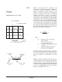
TEST EXAMPLES ................................................................................................................................................................ 29
Airwave Inc.
i
APPENDIX B
MAINTENANCE AND RETUNING PROCEDURES FOR ANTENNA DUPLEXERS..................................................... 35
DUPLEXER TYPES AND OPERATING FREQUENCY BANDS......................................................................................................... 35
Band Pass Type .................................................................................................................................................................. 35
Band Reject Duplexers ....................................................................................................................................................... 35
Pass Reject Duplexer Types ............................................................................................................................................... 36
Pass Reject - Band Pass Duplexers .................................................................................................................................... 36
Duplexer-Isolator Combinations........................................................................................................................................ 36
APPLICATION OF DUPLEXERS .................................................................................................................................................. 36
IMPEDANCE MATCH BETWEEN THE DUPLEXER, TRANSMITTER AND RECEIVER ...................................................................... 37
DUPLEXER RETUNING ............................................................................................................................................................. 37
Test Equipment Requirements ............................................................................................................................................ 38
Tuning Band Pass Duplexers ............................................................................................................................................. 38
Tuning Band Reject and Pass Reject Duplexers................................................................................................................. 40
Tuning Pass-Reject with Added Band Pass Element Duplexers......................................................................................... 40
Tuning Duplexers (“Isoplexers”) with Isolators in Transmit Branch ................................................................................ 41
Hints and Kinks, Errata...................................................................................................................................................... 41
SUMMARY ............................................................................................................................................................................... 41
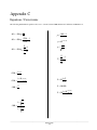
APPENDIX C
EQUATIONS / CONVERSIONS .......................................................................................................................................... 42
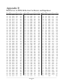
APPENDIX D
RETURN LOSS TO SWR, REFLECTION COEFFICIENT, AND IMPEDANCE .............................................................. 43
APPENDIX E
DBM TO POWER OR VOLTAGE AT 50 OHMS................................................................................................................ 44
APPENDIX F
DECIBELS TO PERCENTAGE GAIN OR LOSS................................................................................................................ 45
APPENDIX G
VELOCITY OF PROPAGATION FOR RG/U CABLE TYPES........................................................................................... 46
Other Cable Types ............................................................................................................................................................. 46
Airwave Inc.
i
Airwave Inc.
1
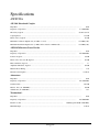
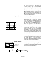
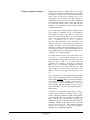
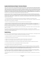
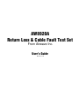
Typical Directivity of the Coupler (Red Trace), as measured on an HP8714B Network Analyzer (blue trace is
calibrated measurement limit of the 8714).
Airwave Inc.
2
Specifications
AW8920A
AW-20-4 Directional Coupler
50 Ω
Impedance ............................................................................................................................................................
Frequency of Operation. ..........................................................................................................................
Directivity, Typical ...............................................................................................................................
0.1-1000 Mhz
See Plot at Left
Coupling Factor ................................................................................................................................................
19.5 dB
Insertion Loss, Typical .......................................................................................................................................
0.7 dB
Maximum Continuous Input Power (at 1 Mhz or more) ........................................................................
+33 dBm (2 W)
Maximum Intermittent Input Power (1+ Mhz, 10 Seconds On, 1 Minute Off) .......................................
+38 dBm (6 W)
AWR-2050 Resistive Power Divider
50 Ω
Impedance ............................................................................................................................................................
Frequency of Operation. ..........................................................................................................................
DC-2000 Mhz
Isolation, Typical ................................................................................................................................................
6.6 dB
Insertion Loss Above 6 dB, Typical .....................................................................................................................
0.3 dB
Phase Unbalance, Typical ..........................................................................................................................................
Amplitude Unbalance, Typical ............................................................................................................................
Matched Power Rating .............................................................................................................................................
Internal load dissipation ..................................................................................................................................
2°
0.2 dB
1W
0.125 W
Attenuators
Impedance ............................................................................................................................................................
Frequency of Operation. ..........................................................................................................................
50 Ω
DC-1500 Mhz
Nominal Value .................................................................................................................................................
Flatness, max. (To 1000 Mhz) ............................................................................................................................
VSWR, max. (To 1000 Mhz) ................................................................................................................................
±0.3 dB
0.6 dB
1.5:1
Termination’s
Impedance ............................................................................................................................................................
Frequency of Operation. ..........................................................................................................................
Return loss, min. .....................................................................................................
DC-2000 Mhz
30 dB (Typical 40 dB @ 500 Mhz)
Maximum Input .................................................................................................................................................
Airwave Inc.
3
50 Ω
0.25 W
Airwave Inc.
4
Unpacking
Kit Contents
The standard AW8920A Return Loss and Cable Fault
Test Kit is supplied with the following Items:
1. Directional Coupler
2. Resistive Power Divider
3. Two (2) 6 dB Attenuators
4. Precision 50 Ω Termination
5. Two (2) Low Loss Test Leads
6. Carry Case
7. Users Manual and Quick Start Guide
Care and Handling
Every effort has been made to insure durability of all kit
components. They remain, however, delicate electronic
devices. The directional coupler is by far the most
sensitive part in the kit. NEVER drop the coupler on a
hard surface, and NEVER remove the cover.
The
physical placement of all the internal parts that make up
the coupler, the wires, transformers, etc. are very critical.
A hard shock to the coupler could adversely affect
performance. Other components of the kit are far less
sensitive to shock, but should be handled with care to
prevent damage to their connectors.
NEVER apply DC current to the directional coupler. DC
current will destroy the coupler and void your warranty.
The minimum frequency of operation for the coupler is
100 Khz, at no more than 0.5 watts below 1 Mhz.
Clean the connectors often using pure TF solvent. The
painted surfaces can be cleaned with glass cleaner.
Warranty
All components of the return loss and cable fault test kit
are warranted to be free from defects in material and
workmanship for a period of one year from the date of
shipment, except test leads, which are warranted for a
period of 90 days. During the warranty period, Airwave
Inc. will at its option, repair or replace at no charge any
kit item found to be defective, provided the item is
returned, shipping prepaid, to Airwave Inc. Airwave Inc.
shall pay return shipping charges to the buyer.
Limitation of Warranty
This warranty shall not apply to any item found to have
been subjected to abuse, misuse, or improper care. NO
OTHER WARRANTY, EXPRESS OR IMPLIED IS
GIVEN.
AIRWAVE
INC.
SPECIFICALLY
DISCLAIMS ANY IMPLIED WARRANTIES OR
WARRANTY OF MERCHANTABILITY OR FITNESS
FOR A PARTICULAR PURPOSE.
Repair or
replacement of the defective item is buyers sole and
exclusive remedy. AIRWAVE INC. SHALL NOT BE
LIABLE
FOR
ANY
DIRECT,
INDIRECT,
INCIDENTAL, OR CONSEQUENTIAL DAMAGES.
Airwave Inc.
5
Airwave Inc.
6
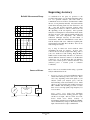
Quick Start Instructions For The AW8920A Test Kit
Return Loss
Connections
Setup
Signal Source
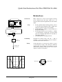
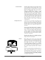
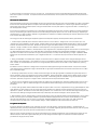
Make connections as shown in the diagram, allowing
power reflected from the device under test to be
separated and measured independently from the incident
signal.
1.
Analyzer Input
2.
3.
Directional Coupler
6 dB
Attenuator
4.
DUT
Normalizing
Normalize the analyzer using “Save B” / “A-B” if
available, or, use a grease pencil or dry erase marker to
trace this reference line on the screen.
Testing
Connect the device to be tested to the “Device” test port
of the directional coupler. The amount by which the
displayed line drops, in dB, is the return loss of the
device under test (DUT). This is plotted on the analyzer
display as a function of frequency.
Device
Under Test
Terminate All
Unused Ports
Set the spectrum analyzer tracking generator controls
to sweep the desired frequency range. Smaller span
settings are preferred for more exact readings.
Set RF Amplitude to 0 dBm (or near the high side of
the generators ability),
Set the input reference level, if available, to -20 dB,
or set the attenuator, vertical gain or position, and IF
gain controls until the displayed line is even with one
of the upper graticules.
Normal Sensitivity at 10 dB per division.
“Tracker” Port
“Analyzer” Port
“Device” Port
Lower Trace = Better Match
Airwave Inc.
7
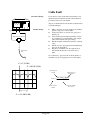
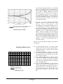
Cable Fault
Automated Testing
If your monitor offers an automated cable fault test, use
the Resistive Power Divider and follow the instructions
provided for this test in your manual.
All ports of the Resistive Power Divider are identical and
can be interchanged.
Signal Source
Analyzer Input
Manual Testing
1)
2)
3)
Resistive Power Divider
4)
5)
Cable Under
Test
6)
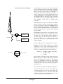
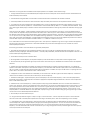
Make connections as shown at left and set tracking
generator output at (or near) 0 dBm.
Connect the cable to be tested to the open power
divider port.
Select analyzer span and input attenuation controls
for a standing wave pattern similar to the example.
(Short cables require wide span settings.)
Find the frequency difference between two adjacent
“dips”.
Find the velocity of propagation from manufacturer
data or from Appendix G.
Plug these two numbers into the equation below
and calculate the distance to the cable end (or
fault).
See “Cable Tests,” page 25 for more details and how to
determine velocity of propagation from a cable sample.
F1 = 67. 625 Mhz
F2 = 202. 03125 Mhz
One-half Speed
of Light
2.54’ =
491.7855 * 0.695
134.40625
Distance in Feet
to Fault
F3 = 134.40625 MHz
Airwave Inc.
8
Cable Velocity of
Propagation
Frequency in Mhz
(See Above)
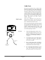
Reflection Measurements
The directional coupler in the AW8920A test kit is a
signal separation device. It provides a sample of the
power traveling in one direction only. The coupler has
three ports, an input port, a test port, and the
measurement sample port. A fourth port is internally
terminated in a precision 50 ohm load.
Measurement
Sample
An incident signal applied to the input or “Tracker” port
of the coupler is passed to the “Device” or test port
unattenuated (less the insertion loss).
Any signal
reflected at this port will be passed back to the input port,
with a sample (20 dB down), directionally isolated from
the incident signal, also present at the measurement, or
“Analyzer” port.
Internal
50 ohm
Termination
Test
Input
Incident
Reflected
Directional Coupler
When compared to the incident signal, This directionally
isolated reflection sample provides the basis for
calculating reflection coefficient, return loss, SWR, and
impedance. (See Appendix D for conversions.)
Reflection Coefficient
Reflection coefficient is the most basic of reflection
measurement values, and is simply the ratio of reflected
power to incident power. This number varies from zero
for a perfect match to one for a total mismatch. If your
spectrum analyzer offers a choice between linear and log
displays, you will be able to read this value directly from
the screen. The symbol for reflection coefficient is ρ
(magnitude only) or Γ (magnitude and phase).
Return Loss
The logarithmic expression of the reflection coefficient is
the return loss, and its value is given in decibels. A
return loss of 0 dB represents a total mismatch, and one
of 40 dB or more, a near perfect match. Since spectrum
analyzers are usually calibrated in decibels, reflection
measurements are read from the screen directly in return
loss. The abbreviation for return loss is RL, R.L. or R/L.
Use the equations
RL = −20 log 10 ρ
ρ = 10
RL
−20
to convert between return loss and reflection coefficient.
Airwave Inc.
9
Impedance
For every measured value of Γ, there is a corresponding
value of impedance. The two are directly related, their
relationship in a 50 Ohm system is shown by the
equation:
Z = 50
1+ Γ
1− Γ
To find reflection coefficient from impedance:
Z
−1
Γ = 50
Z
+1
50
SWR
Reflected signals on a transmission line form standing
waves on the line. Every half-wave along the line, highvoltage and low current points occur. Halfway between
the high-voltage points will be low-voltage, high current
points. The ratio of these voltages or currents is the
Standing Wave Ratio or SWR. SWR is also related to
return loss, impedance, and reflection coefficient, as
shown by the equations:
SWR =
1 + 10 (− RL / 20 )
1 − 10 (− RL / 20 )
SWR =
1+ ρ
1− ρ
and
SWR =
Reflected Power
Z
50
2
2
Since power is proportional to I (or E ), the power
reflected will be proportional the square of the reflection
coefficient, or:
Preflected = ρ 2 Pforward
Airwave Inc.
10
For example, a source impedance of 50 Ω, and load
impedance of 100 Ω, produces an SWR of 2:1 and a
reflection coefficient of 0.3333. The square of 0.3333 is
0.1111, or 1/9, fractional. This means that eight-ninths
of the power indicated by an in-line wattmeter would
actually be delivered to the load. The remaining oneninth is reflected from the load. The reflected power is
reactive power (volt-amperes), and is not actually
dissipated.
Airwave Inc.
11
Airwave Inc.
12
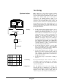
Test Setup
Spectrum Analyzer
Signal
Source
Analyzer Input
Settings
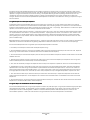
Make connections as shown in the diagram, allowing
power reflected from the device under test to be
separated and measured independently from the incident
signal. The “Tracker” input port of the coupler is
connected to the tracking generator output of the
spectrum analyzer. The “Analyzer” measurement port is
connected to the spectrum analyzer input. The 6 dB
attenuator is used to reduce errors caused by mismatches
between the directional coupler and the signal source. It
should be placed nearest the coupler rather than your
measurement instrument. The “Device” test port should
be left open at this time.
1.
Directional Coupler
6 dB
Attenuator
DUT
Device
Under Test
2.
Terminate All
Unused Ports
3.
4.
Normalized Display
Set the spectrum analyzer tracking generator controls
to sweep the desired frequency range. Use the
smallest span setting that will allow you to see the
desired band, set the bandwidth wider for wide span
settings and for tests on devices connected by long
feed lines. Set the sweep rate quick enough to see
rapid changes on the analyzer display. On the
HP8920A, for example, sweep rate is a function of
the span setting, therefore it is best to use an 18 Mhz
span width rather than 10 Mhz, and 1.5 Mhz rather
than 800 Khz (see HP8920A owner’s manual under
“Spectrum Analyzer” for more on span and sweep
rate relationships in the HP8920A).
Set the RF Amplitude to 0 dBm, or near the high
side of your tracking generator’s output capability.
At this point in the setup, you should see a fairly flat
trace near the top of the analyzer display.
Set the input reference level to -20 dBm. If your
monitor does not have a reference setting, adjust the
input attenuator, the vertical position and IF gain
controls until the displayed line is even with one of
the upper division lines.
Set the display range to read decibels at 10 dB per
division.
Normalizing
If your spectrum analyzer offers a “Save B” / “A-B” or
normalization function, perform that now. Otherwise,
use a grease pencil or dry erase marker to trace the line
on the screen if desired.
Settings Notes
The RF amplitude level is not very critical. Just
remember that there is a minimum loss of 26 dB in the
system when connected as described (6 dB loss in the
attenuator and 20 dB loss in the coupler from the
“Device” test port to the “Analyzer” measurement port;
Airwave Inc.
13
plus any test cables losses).
The analyzer must
compensate for this by using an increased sensitivity
level, or by increasing the generators’ output. With a
higher output level, the spectrum analyzer has a stronger
signal to work with and is easier to use and read.
Although the coupler will operate at levels as high as +38
dBm (at 1 Mhz or above), generator levels about 10 to 20
dB below the highest output level obtainable from your
tracking source (usually between -20 dBm and +15
dBm,) are preferred as this is usually a more stable and
leveled range for the signal generator.
Adaptors and Jumpers
If an adapter or jumper cable must be used between the
“Device” test port and the DUT, connect it now. Keep in
mind that the test set will add any mismatch in the
adapters or jumpers to your reading, effectively limiting
the measurement range of the test setup. A single,
average quality adapter can limit the measurement range
of the test setup to as little as 20 dB. Jumpers longer
than 1/20λ become a part of the DUT, no longer just a
jumper! It is always best to avoid using adaptors or
jumpers whenever possible.
Testing
Once connected and setup as described above, the
spectrum analyzer will display the return loss of anything
connected to the “Device” test port of the set. Since
return loss is a measure of the reflected power from the
device under test, a lower trace on the analyzer display
indicates a better impedance match to 50 ohms. Since
spectrum analyzers are calibrated in decibels, and since
return loss is a logarithmic expression, the analyzer reads
return loss directly.
Lower Trace = Better Match
To see the approximate measurement limits of the test
setup, connect the 50Ω precision termination to the test
port (after following setup procedures as outlined above).
The resulting display is an approximate limit of
measurement. (The actual measurement limit can only be
found by using a special calibration termination.)
Network Analyzers
Terminate All
Unused Ports
Source
It is assumed that most users of our kit will not have
access to an instrument of this class. If you happen to be
fortunate, setup as shown in the diagram and perform the
calibrations as described in your user's manual. By using
a network analyzer, reflection measurements can be made
with great precision and accuracy. Enjoy!
R A
Power
Splitter
DUT
Directional Coupler
Device
Under Test
Airwave Inc.
14
Measurement Procedures
The following are some examples of how the return loss
test set can be used to perform some useful tests. Many
more uses are possible than are listed here. Generally,
any passive network or low power amplifier designed for
50 ohms can be characterized using this return loss test
set. When testing a device with more than one port, it is
important to terminate all unused ports with a 50 ohm
termination. The directional coupler can also act as an
isolating combiner, combining two signals into one with
the signal sources isolated from each other.
The following examples assume that setup and any
calibration(s) as described previously have been
performed.
Cables
Setup the test set with a 0 dB reference line as described
under the section “Improving Accuracy” (page 21).
Attach one end of the cable under test to the coupler.
The other end should be unterminated or shorted, either
way is fine. (Use a shorting termination, not a piece of
wire!) Divide the measurement reading by two to find
the approximate loss of the attached cable and its
connectors. Perform a cable fault check to be sure there
are no breaks in the cable, since this measurement would
not indicate this except in the possible case of abnormal
results.
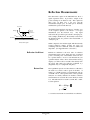
Base Antennas
Before attempting antenna measurements, the location of
the antenna to be tested must be considered. If high
power transmitters are anywhere within a few thousand
feet, it is possible that excessive power may be present at
the connector of the antenna to be tested. This must be
checked before proceeding. Terminate a wattmeter with
a dummy load and connect it to the antenna connector.
Any power measured must be less than 2 watts to insure
safety of the coupler, 1 watt if using attenuators supplied
with the kit, and in most cases, less than 640 mW to
insure the safety of most spectrum analyzers (640 mW
through the 6 dB attenuator results in 160 mW into the
“duplex out” port of the spectrum analyzer). At this
level, measurements can safely be made. Be sure that
any suspect transmitters are operating when you make
this measurement and be sure that your wattmeter is
capable of the full frequency range of all the suspect
transmitters! If the levels encountered are less than 2
watts but greater than 640 mW, a high power attenuator
will be needed. Use a 10 or 12 dB high quality
attenuator, one with good flatness across the frequency
band of interest. Place the attenuator between the
“duplex out” port of the spectrum analyzer and the
“tracker” input port of the directional coupler. If your
Airwave Inc.
15
test set is capable of generating the tracking signal
through a high power test port, it is possible that this port
may be used instead of the attenuator. Usually though,
signals generated from this port will be less accurately
leveled, causing errors in your readings. Avoid this
method if possible. If the levels you encounter are
greater than 2 watts, your only options are to turn off the
offending transmitter(s), or reduce their output power.
CAUTION: The maximum input power at the “Tracker”
or “Device” ports of the bridge is 6 watts under
intermittent operating conditions. Any sustained use at
power levels above 2 Watts could damage the coupler
and will void the warranty. For this reason, 2 Watts is
listed as the maximum input level for the above tests.
The maximum power that may be applied to the
“Analyzer” port of the coupler is 125 mW. Also, pay
attention to the maximum power ratings of the
attenuators. Attenuators supplied with the kit are rated at
1 watt maximum input power.
.
Wide sweep of a good antenna and cable
Once precautions have been taken, the return loss of the
base antenna is measured the same as a mobile antenna.
See below.
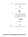
Mobile Antennas
.
Wide sweep of an open or shorted cable
Measure return loss by connecting the test set to the
antenna cable of the antenna under test. The reading is
the same quality of match the transmitter or receiver
“sees” when connected to the transmission line, and is a
composite signal of the return loss of the antenna, the
cable, any connectors, any losses, and a standing wave
pattern related to the length of the cable between the test
set and the antenna, and finally, the match at the end of
the cable (the antenna). Whew! For most purposes, this
reading is enough to determine whether or not you have a
problem. If the RL reading seems poor, increase the span
of the spectrum analyzer (or vary the center frequency up
and down) enough to see the composite wave effect of
the antenna and cable. Poor RL with no wave pattern
may indicate an open or shorted cable (pattern may be
very difficult to see with short antenna cables). It is also
possible that if the transmission line is cut to the wrong
fraction of a wavelength at the frequency of interest, the
standing wave pattern on the feed line can make an
acceptable RL from the antenna appear unacceptable at
the end of the cable. By just shaving a few inches off the
feed line (or by changing the length of a jumper), the RL
that the transmitter or receiver “sees” can, in some cases,
be improved. A SWR reading of 1.5:1 is equal to a
return loss reading of 14 dB. In most cases, this is the
value that manufactures specify as a minimum
performance level for their antennas.
The usable
bandwidth of such an antenna, is the span between the 14
dB points.
Airwave Inc.
16
Portable Antennas
Although portable antennas can be measured using this
test set, obtaining an accurate reading is tricky. A test
fixture must be made to hold the antenna over a ground
plane that simulates a portable radio in real world use.
Except for manufacturing, this may not be an
economically feasible venture compared to simply
replacing a suspect antenna. To do a simple test, connect
the antenna to the coupler test port through an adapter, if
needed, and watch the analyzer display. Hold the
coupler with the antenna near your head, as if it were on
a radio in use. Notice the degree of signal variance with
only small changes in how the coupler is held in the
hand! After testing several known good antennas, you
should at least have an idea of what to expect when
testing unknowns.
Preamps and receivers
Connect the test set to the input of the preamp or front
end to be tested. In the case of the preamp, terminate the
unused port with a 50 ohm termination. If the receiver
front end is part of a transceiver, disable the transmitter
before proceeding. It is also important to apply power to
the preamp.
The trace on the analyzer display is the plot of return loss
versus frequency, tune the front end for a minimum of
about 14 dB RL across the entire operating band of the
device, or for the best reading possible at the frequency
of interest. Usually, only the slugs or trimmers preceding
the first amplifier can be tuned with this method.
Disconnect the test set and continue tuning the remainder
of the device conventionally.
The RL at the output port of a preamp can also be
measured if the power levels involved do not exceed the
ratings of the test set or the analyzer.
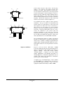
Isolators
Signal
Source
Analyzer Input
Input
6 dB
Attenuator
Isolator
Output
6 dB
Attenuator
Before tuning, test the isolator at the factory tuned
frequency and make note of its performance: Measure the
insertion loss of the isolator both forward and reversed.
Then measure the return loss at the input and output
ports. Make sure the isolator load is connected!
Compare this performance with the isolator after retuning
to be sure performance is acceptable. Also, be sure to
perform an RL test of the isolator termination(s) to be
sure of their acceptable performance (RL of 26 dB is
optimal).
Set up your spectrum analyzer and tracking generator as
shown. The 6 dB attenuators serve to move the
measurement plane directly to the isolator, and remove
the test leads from the measurement. This setup is
recommended if the test leads exceed 1/20 λ. Remember
to account for the 12 dB loss in your readings, or perform
a normalization function with a
Airwave Inc.
17
barrel connector in place of the isolator. Set the sweep
width to cover both the old frequency and the new
frequency, if possible. Tune capacitors C1 and C2 (C1,
C2, C3, and C4 for a dual isolator) to move the pass band
from the old frequency to the new, tuning for lowest loss.
Reduce the sweep width and continue adjusting until no
further improvement is noted. The fall off response
should be fairly symmetrical above and below the tuned
frequency. Reverse the connections at the isolator and
adjust C3 (C5, and C6 on a dual) for highest loss.
C2
C1
Input
Output
Single Isolator
C3
C1
C2
C3
Now terminate the isolator output port with a precision
termination. Set up for return loss measurement and
measure return loss at the input port of the isolator and
tune capacitors C1 and C2 (C1, C2, C3, and C4 for a
dual isolator) for best return loss at the transmit
frequency. Only minor adjustment should be necessary,
and a RL of around 26 dB should be the goal. Now,
reverse the connections at the isolator; place the
precision termination at the input port, and the
measurement set at the output port. Adjust C3 (C5, and
C6 on a dual) for best RL at the output port. Again, only
minor adjustments here for around 26 dB or better RL.
C4
Output
Input
C5
C6
Dual Isolator
We recommended this method of tuning (conventional
first, RL second) because it is possible for an improperly
tuned isolator to exhibit a seemingly acceptable RL (the
applied signal is dissipated primarily within the isolator).
Unacceptable insertion losses and performance would be
the result.
Duplexers and Filters
Duplexers and Cavity Filters-- Bill Lieske, of EMR
Corporation in Phoenix Arizona, has written what may be
the most comprehensive guide available on the subject of
duplexer retuning.
From Mr. Lieskes’ manual
“Technical Papers,” a complete copy of the chapter
entitled “Maintenance and Retuning Procedures for
Antenna Duplexers” is included in appendix B. We are
grateful to Mr. Lieske for his permission to include this
work as a part of our user manual.
A complete copy of “Technical Papers,” can be obtained
by calling EMR Corp. at (602) 581-2875. Also ask for a
price list and catalog of products. Some of the best
equipment available in the industry is Made at EMR.
Airwave Inc.
18
Site Noise and Receiver Sensitivity
The sensitivity of a receiver on the “bench” will always
be better than the same receiver connected to an antenna,
due to “site noise." Power lines, nearby transmitters,
sunspots and other sources of noise are everywhere. So
how do these noise levels effect receiver sensitivity? To
find out, set up the test set as in the diagram. Be sure any
associated transmitter(s) on the same line as the coupler
are disabled for this test, and it may be wise to measure
the received power at the coupler insertion point (see
“base antennas” section above for details) before
proceeding.
Adjust the generator output for 12 dB receiver SINAD
with the termination in place, and compare the generator
level to that required to obtain a 12 dB SINAD with the
antenna in place. Remember that the coupler has about a
20 dB loss in-line with the generator, so subtract 20 dB
from the measured values to find the actual generator
levels, if desired.
Signal
Generator
Termination
Receiver
The difference between the two noted generator levels is
the amount by which the site noise degrades the receiver
sensitivity. So, to find the actual receiver sensitivity of
the system during use, take the antenna system gain (or
loss), minus the site noise as determined above, and
subtract the results from (or add them to) the receiver
“bench” sensitivity.
Rx Sens. = “Bench” Sens. - (Ant. Gain or Loss - Noise)
Example: An antenna with 10 dB gain is used with a
cable having a loss of 3 dB. The measured site noise
degradation is 4 dB, and the bench sensitivity of the
receiver is -118 dBm. The actual system sensitivity is:
“Tracker” Port
Rx Sens. = -118 dBm - (+10 dB - 3 dB -4 dB)
= -118 dBm - 3 dB
= -121 dBm
“Analyzer” Port
“Device” Port
In this example, if the cable is replaced with one having 1
dB loss (instead of the current 3 dB loss), the measured
site noise would increase by 2 dB, to 6 dB, (since site
noise is also attenuated by cable losses). The resulting
system sensitivity would be... -121 dB! Thus, system
sensitivity would not necessarily benefit by upgrading the
transmission line.
As can be seen, this could be a valuable test to perform!
Note also that site noise is not a static value, but is
constantly changing, day by day, and varies with the time
of day and the time of year. Site noise studies must
therefore be conducted over a long enough period of time
to be sure the results are true and reliable.
Airwave Inc.
19
Airwave Inc.
20
Improving Accuracy
Reliable Measurement Range
A consideration in the quest for precision is the
resolution and accuracy of your display instrument. Most
low cost spectrum analyzers (the kind found in
communications service monitors, and the kind for which
this test set was primarily intended) will yield excellent
results when measuring return loss from between 5 to 30
dB -- and will provide reasonable accuracy when
measuring from around 1 or 2 dB to as much as 40 or 45
dB, depending on the test frequency. Most spectrum
analyzers are inadequate for measurements much outside
this range, however. They lack the tracking stability and
resolution, and most importantly, the advanced
calibration techniques necessary for that latitude of
measurement. When the AW8920A kit is used with a
network analyzer with vector calibration capability, RL
measurements from 0.001 dB to 60 dB or more can be
made with great accuracy.
Try to keep in mind real world situations when
determining the need for accuracy. In most cases,
someone else has already designed the thing, and it’s
your job to decide if it’s still working. Keep the RL to
SWR conversion table handy and refer to it often. Note
that the difference between a return loss of 30 dB, when
compared to one of 40 dB means that only 0.0898%
more of the forward power is reflected from the load
(reflected power = forward power x reflection
coefficient ).
Sources of Errors
Most of the errors encountered when using a spectrum
analyzer with this kit are from:
•
MEASUREMENT
ERRORS
Measured Data
Z?
Frequency response errors from within the analyzer
and the interconnecting cables to the test set. These
errors vary, depending on the actual quality of your
analyzer (check your analyzer specs,) and the
interconnecting cables used with the test set. Their
effects are most noticeable with readings between 0
dB to 5 dB RL. The best thing you can do to reduce
these errors is use high quality, high frequency low
loss test cables.
Source match errors result from impedance
mismatches between the tracking generator output
and the test set input. This is a minor error term.
Source match errors affects accuracy of
measurements primarily between 0 dB and 5 dB RL,
and are minimized by using a 6 dB attenuator at the
input of the directional coupler. When the kit
Unknown
Airwave Inc.
21
is used with the supplied attenuators, the maximum
effect of source match error on an RL reading of 5
dB is about ±0.5 dB, increasing to about ±0.75 dB
for a reading of 2 dB RL. Experience has shown
that these errors are almost always less than the
above maximums, and unless you are using a
specialized spectrum analyzer or network analyzer,
are usually insignificant compared to the frequency
response errors almost certain to exist in your
measurement instrument.
-4
-2
0
+2
+4
0
•
10
20
Measured Return Loss dB
30
40
Max. Source Match Error (using supplied attenuators)
Max. Directivity Error (at 40 dB directivity)
Measurement Uncertainties
Directivity error is the collective imperfections
within the directional coupler that allow a signal
from the source to “leak” directly to the
measurement port, and limit the directivity of the test
set. Directivity error is the most significant error
term for RL measurement. Directivity Error limits
the effective measurement range of the test setup and
contributes errors to readings primarily beyond 25
dB RL. With an RL reading of 25 dB, directivity
error will contribute an uncertainty of about ±1.0 dB,
and at an RL of 35 dB, uncertainty of about +3 to -2
dB. As a rule of thumb, if the directivity of the
coupler is about 10 dB greater than the reading at the
frequency of interest, the measurement will be
reasonably accurate.
Be sure to see the measurement comparison test results in
the appendix.
Establish a Reference Line
Open Termination
0 dB Reference
Shorted Termination
0 dB Reference Line
1) To obtain the highest degree of accuracy possible
from the return loss test set, setup as usual, without
attaching any adapters or jumper cables (if needed)
to the test port just yet.
2) Normalize the display by performing the “Save B” /
“A-B” analyzer function if available, or by tracing
the displayed line on the analyzer with a grease
pencil or dry erase marker.
3) Next, establish a 0 dB reference as follows. Connect
a short circuit termination (not included with the kit)
to the test port. One-half the return loss measured
for the short circuit termination from the normalized
line, is the 0 dB reference.
4) If you are using an HP8920A, you can enter this
number as the “reference” at the menu field “Lvl” If
your spectrum analyzer does not have a reference set
function, make a note of the 0 dB reference point, or
use a grease pencil to trace a reference line on the
analyzer screen. Reference your test results to this
line.
Airwave Inc.
22
Using an Adapter or Jumper
When using an adaptor or jumper at the test port, signal
reflections from impedance mismatches and losses within
the adaptor or jumper tend to limit the measurement
range of the test setup and contribute errors to the
measurement. If for instance, the adaptor exhibits a
small inductive reactance, and the test device exhibits an
equal capacitive reactance, the two will cancel each other
out. The result will be either a better than expected
reading, or worse depending on the non-reactive element
of the DUT impedance.
It is also important to understand that if a jumper is used
whose length is a significant portion of a wavelength at
the frequency of interest, longer than, say, 1/20 λ, the
return loss being measured will not be of the intended
device. The measurement will instead be of the test
cable, as terminated with a device of unknown
impedance (this information is very useful if the “test
cable” also happens to be the feed line to an antenna, for
example). In order to obtain an accurate measurement
under these conditions, the phase relationships and losses
involved must be known. Using this information along
with a Smith chart and a little math, the jumper can be
“calibrated out” of the measurement.
It is assumed that most users of our test kit will not have
easy access to a vector analyzer, and therefore, it is
recommended that all test leads at the device port of the
bridge be kept to 1/20 λ or less (This limits the
practicable use of jumpers to frequencies of around 50
Mhz or less). It is preferable to lengthen the test leads
from the analyzer to the coupler, and then use a high
quality adapter at the device port, if necessary. If an
adapter is used, have the right one handy and use only
one.
If you would like to see the approximate measurement
range of the test setup with an adaptor or jumper in-line,
attach (using no further adapters) a precision termination
to the end of your adapter or jumper. Unless you have a
good selection of precision termination’s, this is not
always possible. The trace displayed is the approximate
measurement limit of your test setup with the adapter or
jumper in-line.
To find the true measurement limit of the test setup, a
specially made calibration termination must be used.
Airwave calibration terminations exhibit a nearly flat RL
of about 50 dB. They are available for N, SMA, and
BNC connector types, and are priced according to the
difficulty involved in construction and tuning (inquire).
Calibration terminations are rarely necessary and used
mostly for laboratory work. The termination included
with the kit is suitable for nearly any application,
including most manufacturing situations.
Airwave Inc.
23
Airwave Inc.
24
Cable Tests
The resistive power divider is used to combine a swept
signal from a tracking generator with a reflected signal
from the cable under test. The resultant standing-wave
trace on the analyzer display can be used to find such
information as distance to a fault, velocity of propagation
of a known length of cable, and the exact length of cable
needed to form 1/4 λ, 1/2 λ, etc. stubs or jumpers. Some
service monitors such as the HP8920A, the IFR-1500, the
Motorola 2600, and others offer built-in cable fault
checking. These monitors use the FFT to find the
distance to a cable fault.
Fault Location
When using the HP8920A, run the cable fault test
program from the “Tests” screen and follow the
instructions provided with the software “System Support
Tests.” Instructions are provided on screen.
Other service monitors that offer a cable fault test function,
such as the IFR-1500 and IFR-1200 Super S may benefit by
substituting the resistive power divider in place of a “T”
connector specified in the instruction manual. This
presents a 50 ohm impedance not only to the service
monitor ports, but also to the cable under test, allowing a
more accurate pinpointing of the fault.
Signal
Source
Analyzer Input
Test Setup
1)
Connect the tracking generator output to “Port 1”
of the power divider, the analyzer to “Port 2,” and
a precision termination to the “Source” port (note
that all ports of the Resistive Power Divider are
identical and can be interchanged, labeling is for
convenience).
2)
Set the tracking generator and spectrum analyzer
to the widest sweep possible. The generator
output should be as high as possible, but not
greater than about 10 dBm.
3)
If your spectrum analyzer offers a normalization
function, set the input attenuation for the analyzer
to match the generator output (+10 dBm output,
10 dB attenuation) and normalize the display.
4)
Now set the analyzer input attenuation to a level
10 to 20 dB higher than the signal generator
output. The trace displayed should be relatively
flat, and about a graticle or two from the top line.
Resistive Power Divider
Cable Under
Test
Normalize with
Termination
Airwave Inc.
25
Testing
Example:
Display Results of a 2’ 6.5” Cable.
F1 = 67. 625 Mhz
F2 = 202. 03125 Mhz
When an unterminated cable is connected to the
“Source” port, a standing wave pattern is displayed on
the analyzer screen whose frequency of repetition is
related to the length of the cable under test or the
distance to a fault. The longer the cable the higher the
frequency of repetition. If the span of the spectrum
analyzer you are using is too narrow, or the length of
cable under test is too short, this pattern may not seem
evident at first. Using an IFR 1200 for example (10 Mhz
span maximum), any cable less than about thirty-five feet
long will be too short to see the standing wave pattern.
To view the wave, the center frequency of the generator
can be varied to find a “dip” in the analyzer trace. Make
a note of this frequency, and find the next adjacent dip,
then calculate the frequency difference between the two
dips. This is the half-wave frequency. The length of the
cable can now be found by the following:
D = .5 c Vr
f
(1)
Where:
F3 = 134. 40625 Mhz
D
c
Halfwave
Frequency
.Vr
f
One-half Speed
of Light
2.54’ =
Cable Velocity of
Propagation
491.7855 * 0.695
134.40625
Distance in Feet
to Fault
Frequency in Mhz
(See Above)
= Distance to fault or end of cable
= Speed of Light,
= 983.571 for ft per second, or
= 299.792 for m per second
= Velocity of Propagation of the cable
under test
= Frequency in Mhz determined by
the above test and calculations
The speed of light is expressed in feet or meters per
second, and will yield results in the same unit of measure.
The Velocity of Propagation can be determined from the
table in the appendix, or experimentally as described
below.
Example: Consider the example shown at left. This was
a section of RG/U 142 cable with a measured length of
exactly 2.5417 feet (2’ 6.5” ), including connectors. The
measured frequency of the first dip is 67.625 Mhz; the
second dip is at 202.03125 Mhz. The difference between
the two is 134.40625 Mhz; this is the half-wave
frequency. The published Velocity of
Airwave Inc.
26
Propagation for RG/U 142 is 69.5%, plugging into the
equation:
D=
=
491.7855 * 0.695
134.40625
341.790
134.40625
= 2.543 ft
As can be seen from this example, the results are quite
accurate.
Velocity of propagation
The Velocity of Propagation is the speed at which the RF
signal travels through a cable. This number is required to
find the distance to a cable fault as described in the
previous section. It follows then, that if all other
quantities are known in the equation above, Velocity of
Propagation can be found from the equation:
.Vr =
D* f
.5c
Using the numbers from the previous example:
.Vr =
2.543 * 134.40625
491.7855
= 0.695
This is the published Velocity of Propagation number for
this cable.
See appendix for RG/U Velocity of
Propagation table.
Once you have found Vr by using a known length sample
of the cable to be tested, you can then perform the
distance-to-fault test as described previously.
Airwave Inc.
27
Cutting Cable to a Desired Wavelength
Sometimes it is desirable that several cables be trimmed
to have a particular electrical length, such as when
preparing interconnecting cables for a duplexer or
isolator. Half wavelength cables present a well matched
source and load with phase relationships delayed but
essentially unchanged. A quarterwave stub can be useful
for suppressing interference at the tuned frequency, and a
length of cable can often serve as an impedance
transformer to match a mismatched source and load.
Preparation
Set up the test set as described in the previous section
entitled “Cable Tests”.
1. Using the following equation, calculate the
approximate length of cable needed for the desired
wavelength ( λ) of cable at your desired frequency
( f ).
Standing Wave Pattern of Unterminated Cable.
Length feet = ( λ)
(983571
. )(Vr )
f
or:
Length Meters = ( λ)
(299.792)(Vr )
f
See Appendix G to find the velocity of propagation
(Vr) for many cable types.
Cutting
2.
3.
Measure your cable length from the above equation,
plus a little extra to account for Vr variations. If you
are making a jumper, and the length of cable you
will need is longer than your calculated length; cut in
multiples of the calculated length, plus a small
amount to allow trimming.
Install one connector to the cable and connect to the
test setup. Set the center frequency of the monitor to
the “dip” frequency found from the following:
frequency cut = 0.25
Same Cable, Terminated in Short Circuit.
4.
Airwave Inc.
28
f
λ
Trim the cable for a “dip” on the display, making
sure that the cut end remains open (not shorted)
during measurements. Keep in mind that the length
of any adapters used at the test port, or connectors
not yet installed will add length to the cable. These
lengths are more significant at higher frequencies.
Appendix A
Test Examples
The following examples are of actual measurements made using the AW8920A test kit. An HP8920A communications test
set and an HP8714B network analyzer were used to produce the hardcopy.
View of the screen prior to performing normalization, (HP8920A).
Same test setup after performing a “Save B” / “A-B” normalization function.
__________________________________________________________________________________________________
Airwave Inc.
29
Test set is terminated with a precision termination, showing the approximate measurement range.
Same termination, with an adaptor in-line.
__________________________________________________________________________________________________
Airwave Inc.
30
Transmission characteristics of a band-pass filter.
RL reading of the same filter at the same frequency and span.
__________________________________________________________________________________________________
Airwave Inc.
31
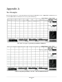
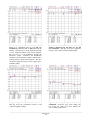
Above is a comparison plot of a 2.0 dB test
termination performed with an HP8714B network
analyzer. The blue trace is of the termination through
a vector calibrated channel of the network analyzer.
The red trace is of the termination through the
directional coupler, normalized but uncalibrated
(identical to the reading that would be obtained with a
tracking generator and spectrum analyzer). This plot
shows the comparative accuracy of the coupler at lowlevel RL readings.
Another comparison plot, this time of a 16.3 dB
test termination. This plot shows the comparative
accuracy of the coupler at mid-level RL readings.
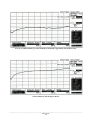
Comparison plot of a 39.8 dB test termination.
This plot shows the comparative accuracy of the
coupler at high RL readings.
Expanded scale comparison plot of a 16.3 dB test
termination. Notice the scale of the reading, and
how closely the coupler (red) trace matches the
vector calibrated (blue) trace.
__________________________________________________________________________________________________
Airwave Inc.
32
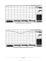
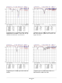
Comparison plot of a 800 Mhz portable antenna,
measured in a test fixture. Notice that the span
width has been increased to center the traces.
Comparison plot of a UHF yagi with a 54 ft feed
line. The interference pattern seen is related to the
length of the cable.
Comparison plot of a UHF yagi antenna with a 2ft
feed line.
Comparison plot of a VHF mobile antenna on a
mag-mount base with 12 ft of cable.
__________________________________________________________________________________________________
Airwave Inc.
33
Cable test standing wave pattern.
Automated test of fifty foot cable. Measurement made on the HP8920 running “System Support Tests” software.
__________________________________________________________________________________________________
Airwave Inc.
34
Appendix B

#
"
#
"
$
#
#
# #
!
$
&
'
(
%
#
#
"
) *
)
$
#
"
%&
+
&
+
+
'
$
$
"
%
+
#
%
/
#
#"
,
*
,
"
*
#
#
,
%
%
#
.
% .
$
"
%
*
#"
%
#
$
" %
,
"
%
2
33'34
#
# $'
"
#
"
"
%
=
, #
*
#
"
, = $
*
,
#
# # $
/ 44'564
"
"
#
"
#
"
,
#
,
*
0
#
'
#
1
+
%
"
#
,
"
"
,
,
% "
"
"
#
1
, "
*
$2
573'586 / 963'986 / 986'85: 463'4;3 /
4;3';36 /"
463'4:5<485'433 /
4;3';65<;78';96 /1
# "
1
, #
#
'
,
#
"
, " %
$
#
#
#
$
$
+ #
" %
#
*
'
"
"
*
"
"
#
"
#
"
#
"
/ 554'573 /
, "
"
#
, "
68
, -> .
"
#
$'
#
"
,
+
$
#
*
,
"
"
#
#
0
,
,
"
#
%
#
, "
$
,
,
" %
*
$
$'
#
"
,
*
+
$
#
*
#
, =-
.
#
#
% 573
"
$
#
"
"
,
"
,
*
#
+
"
%
%
#
*
%
/
*
,
"
"
*
"
?
#
/
#
,
,
,
"
$
#
%
#
"
#
,
#
,
#
,
#
"
,
#
=
#
,
,#
,
,
"
+
"
# 573
/
;36
/
#
/
__________________________________________________________________________________________________
Airwave Inc.
35
+
$
$
#
#
#
=
.
"
"
+
,
0
" ,
,
"
#
#
,
"
%
"
%
%
#
*
,
#
,
/
#
$ "
"
#
"
,
,
"
"
,
# 573
;36
"
,
+
,
"
#
,
,
,
#
"
)
#
,
/
#
#
86
' +
#
%
"
,
#
,
,
%
"
+
$'
"
#
%
"
#
"
#
"
##
#
#
,
'"
# "
*
"
#"
$
)
5
" %
#
#
@
#
'?
:
%
"
#
"
"
#
'
,
# #
?
+
"
"
/
$
"
#
#
+
+
"
,
%
573
,
" ,
#
#
/
#
%
%
%
,
#
#
#
" #
#
#
-
,
, .#
%
,
#
#
#
#
# %
"
,
,
$
#
#
&
#
,
,
7
" %
$
,
"
*
%
#
+#
"
" %
!
,
,
%
"
:
:
68
%
%
#
#
C
$
C
#
'
-?
#
%
"
#
#
-
"
.
*
#
.
#
#
+
%
+
+
7
8
#
#
?
#
"
"
!
5:;3
"
#
"
"
#
,
"
" %
3
$
# D8
#
!
##
5:6
"
,
# '"
#
!
,
#
" #
#
#/
%
*
*
#
:
"
"
" ' '
#
?
/
B
"
,
#
B?
%
#
#
$C
"
#
#
+
*
= $2
,
#
" %
"
) "
)
"
67
,
%
%
% #
A
,
%
) "
0
#
"
#
#
*
*
" %
#
#
%
#
$
%
+
*
#
#
,
C
*
%
+ #
,
,
,
#
"
*
"
"
E10 =
*
,
% ,
"
#
#
%
,
"
#
#
,
#
__________________________________________________________________________________________________
Airwave Inc.
36
?#
%
(
$
#
% "
#
#
#
86 #
#
%
, )
5<9% ,
#"
%
(
86
#
% ,
%
# #
%
"
%
# #
#
" #
%
" # #
%
#
"
%
$
#
+
: C
+#
"
7
%
#
#
%
=
*
# #
+ " #
" - ?. %
,
##
#
+
$
"
+
#
"
A%
86( #
+#
#
"
B
#
#
#
#
566%
"
# #
46%
%
#
,
$
"
$
"
%
"
#
%
?
" %
%
%
#
"
, "
"
"
,
"
"
%
,
,
$
#
+
5:
1?C
,
#
,
#
#
*
*
#
#
,
,
%
#
#
"
#
&
#
#
*
"
"
%
7
,
+ #
, %
#
"
*
3 $
"
%
#
?
#
"
%
/
1
%
0
%
%
,
*
+
+
"
#
/
#
"
"
#
466
# #
#
# #
&
/"
"
#
5G
B
#
$'
*
#/
A
#
*
&5 8
%
"
"
/
586
/
*
B
#
"
.
#
#
%
% #
,
-
"
,
D'4
"
$'
#
+#
,
*
"
#
#
AC
#
*
#
" # ,
986 /
/
%
#
"
"
#
%
#
&?
A
"
98
" " "
" %
#
B
#
$
"
86
%
5 :&5
,
#
#"
, %
+
#
8
%
86 # #
$
%
" %
5
#
9
"
#
)
%
#
,
%
'
#
#
#
"
"
%
#
#
#
: $
,
,
#
,
,
"
"
%
# "
#
'
5 1
%
#
#
$
%
,
%&
5 )
#
"
%
#
:&5
#
8
E10
#
+
,
#
+#
$
%
%
#
#
*
%
#
$
# #
%
9 F
#
,
#
%
#
"
#
#
"
=
"
__________________________________________________________________________________________________
Airwave Inc.
37
0
%
%
'
=
?
?
% % %
#
%
"
% %
#
"
"
$
*
#
*
#
,
, #
) % % '%
*
$
1
"
,
,
#
,
% "
#
% ,
#
/
/
#
#
,
#
#
%
"
%
#
#
"
#
#
,
*
+
%
*
"
"
#
"
68
%
D8
#
,
+ #
5:6
"
+ #
"
%
5
,
,
#
#
#
,
#
*
%
% ,
#
/
*
" %
?
,
1'
1
%
"
/
+
56
,
"
# J:8666
#
#
#
,
86
)"
" H %
"
#
#
46
#
#
65
* #
&
'
96
#
566
/
*
#
"
1 % /@
% ,
#
#
%
"
"
%
0 ,
"
* #
"
=#
% '%
?
I
#
# +
JD8666
#
0
$
#/ #
K
:
,
-
"
" % ,
.?
*
86H/ "
-"
.#
$
#
,
#
,
#/
,
#
,
# #
*
*
)"
"
!H)
#
86
$C
"
3
1(':7;B
%
#
@
*
, -!H).
#
,
#
"
"
"
#
1,
/ %
"
"
, 46
"
+"
#
"
46
, E10 A
% $
C
C
% "
,
E10
5 68&5
#
,
,
"
"
#
%
/
:
%
#
% ,
#
"
%
"
#
B
E10
#
#
#
"
%
*
"
%
!H) *
!H)
-
"
#
#/
#
#
#
*
(
# "
+
"
"
EH)
#/
"
$
,
#
"
"
%
#
#
#
"
%
,
5
#
,
+
=#
#
/ %
/
"
46
)"
,
"
, #
*
#
#
#
,
86 # "
#
#
*
%
8 ?
"
*
7 1,
9 $
/
"
"
#
*
% "
.$C 1
#
%
%
-!H).A ':84
"
$
$
#
# " ,
"
,
*
(",
"
,
+ #
# +
*
*
"
#
0
#
$
,
"
6 8G
"
#
'
"
+ #
,
,
#
+ #
%
"
__________________________________________________________________________________________________
Airwave Inc.
38
# #"
%
#
5 $
,
"
,
: $
%
7 $
"
#
"
'
"
%
%
#
#
/
*
%
#
: $ #
"
#
8
"
,
,
%
#
" %
#
B
#
%
,
, =
#
#
5 8&5E10
#
8G
#
E10 =
# #
%
,
#
*
,
#
%
&
5# '%
A6
B
%
"
,
"
A0
) #
"
#
'
#
*
%
+
#
/ !H)
# "
,
"
#
, = *
%
;8
3 / 466' ;36 /"
#
,
,
"
#
" %
C
,
#
B
% "
"
%
5 5&5
#
,
#
3 ? * #
,
#
#
<
+
*
#
5 5&5
#
,
#
"
%
/ "
) 5:8%
5 / EH) 7
A E10
#
(",
#
%
#
:3
,
,
%
*
+
#
, =
#
#
"
"
#
,
,
%
#
7 1
D
"
"
E10
"
A
#
##
5 C #
/
%
?
, "
%
9
%
#
#
#
%
" %
"
%
$
#
, "
#
#
% %
% "
=
59 B "
% % "
%
%
"
#
# #
#
5 8&5A
%
:6G
:3
#
#
(
%
%
"
#
E10 =B #
A
?
"
&
,
%
9
#
, "
,
,
,
)
#
566%
+
5:6
<
$2
:3
%
?
$
$'
#
*
"
D8
,
*
*
,
*
%
%
B
"
,
=
#
*
#
*
C %
,
+ #
#
#
4 ("
,
<
%
0
#
"
%
"
*
#
+
"
#
-
;
,
,
#
55 ?
#
,
#
=
%
"
# # C
C
?
-" #
.
F
,
$2
#
#
,
#
*
#
*
" #
?
*
%
,
"
2
56 !
"
" %
##
#
.
#
,
"
"
"
#
,
,
#
/
#
"
:3
5
#
*
2"
#
,
*
#
?
4
"
# , %
L
#
*
"
$
%
+
0
"
*
#
#
# %
L
"
" %
#
%#
,
%
$
# #
+
__________________________________________________________________________________________________
Airwave Inc.
39
? % "
*
#
"
%
#
*
#
#
,
$
#
#
"
*
#
##
"
"
0
##
,
"
#
0
?
,
" #
#
#
"
#
#
$
+
,
#
1#
+
#
%
"
,
"
%
"
0
->.#
"
586 /
% A
%
, "
%
#
%
#
%
"
$'
%
#
,
/
+
#
9 0
,
8 C %
,
,
,
,
*
%
:
+
8 C
,
4
#
#
$
'
$
,
,
#
#
" :3
?
##
*
+
+
#
=
#
?
#
+
#
+
,
%
*
"
+
,
# %
,
"
#
,
#
+
#
,
#
=
#
%
#
86
,
"
#
,
,
("
'
, 0
#
$
#
"
*
"
+
%
, " %
# '"
#
"
%
*
#
"
,
$ %
*
,
*
#
, #
" :3
C
#
D C %
,
*
#
,
#
#
#
%
*
#
#
3
,
,
546' :66F /
#
#
%
%&
#
#
#
,
,
%
#
' +
"
,
38
%
%
#
#
%
,
"
# "
0
"
,
,
"
#
#
"
,
*
,
,
$'
,
7
,
*
=
##
:
%
$'
*
"
C
B
#
5C #
,
$'
%
$
#
$
# %
,
%
%
#
#
#
,
*
"
,
'
%
, %"
,
"
#
#
,
*
%
#
#
+
,
,
' +
##
5:6
@
,
#
"
#
#
"
__________________________________________________________________________________________________
Airwave Inc.
40
$
A-?
.B%
?
$
#
)
%
'
5
,
#
'
A
AB
: C %
*
%
#
B
# B
%
,
#
7 ?
*
%
&?
"
H
,
:
#
AB
,
:2
#
=
"
'
+
+
A
+
+
C
"
%&
*
*
#
,
%
#
#
*
M7 " ,
F
(
"
+
#
"
,
,
"
#
% " "
,
"
"
?
$
"
*
,
A
B
,
,
: 1
*
"
*
?
+
(
% "
"
(
#
,
#
#
*
%
1
#
"
+
&6 8
,
" 54
"
C %
#
,
"
,
("
5
58
,
,
"
#
,
# 53
"
:8
% "
,
*
,
->.
"
"
"
"
#
7 ? % "
"
%&
#
%
+ #
"
#
,
,
$
"
#
+ #
"
C
+ "
5 ?
"
"
,
"
,
'
"
#
+
,
"
,
"
"
"
%
#
#
,
,
,
, "
"
#
" #
0
#
#
# #
"
,
"
1 ##
,
#
%
#
%
#
"
*
, %
,
/ ,
*
# #
'
#
"
"
#
#
,
# #
,
,
$
#
"
C
#
#
*
#
%
#
%
#
*
# "
(
=
# "
#
$
,
# #
%
$
"
#
#
#
#"
#
#
#
,
H
#
"
*
"
%
#
#
,
"
"
%
#
"
%
%
#
0
,
#"
,
566G
__________________________________________________________________________________________________
Airwave Inc.
41
Appendix C
Equations / Conversions
The following mathematical equations allow one to convert between SWR, Reflection Coefficient, and Return Loss.
RL = −20 log10 ρ
RL = −20 log10
SWR − 1
SWR + 1
Z
−1
RL = −20 log10 50
Z
+1
50
ρ=
SWR − 1
SWR + 1
ρ = 10 (− RL / 20 )
ρ=
Pr
Pf
Z
−1
50
Γ=
Z
+1
50
SWR =
1+ ρ
1− ρ
SWR =
1 + 10( − RL / 20)
1 − 10( − RL / 20)
Z = 50
SWR =
Z
50
Z = 50SWR
1+ Γ
1− Γ
Z = 50
1+
SWR =
1−
1 + 10 ( − RL / 20)
1 − 10( 1RL / 20)
Pr
Pf
Pr
Pf
__________________________________________________________________________________________________
Airwave Inc.
42
Appendix D
Return Loss to SWR, Reflection Coefficient, and Impedance
RL
40.0
39.8
39.6
39.4
39.2
39.0
38.8
38.6
38.4
38.2
38.0
37.8
37.6
37.4
37.2
37.0
36.8
36.6
36.4
36.2
36.0
35.8
35.6
35.4
35.2
35.0
34.8
34.6
34.4
34.2
34.0
33.8
33.6
33.4
33.2
33.0
32.8
32.6
32.4
32.2
32.0
31.8
31.6
31.4
31.2
31.0
30.8
30.6
30.4
30.2
30.0
29.8
29.6
29.4
29.2
29.0
28.8
28.6
28.4
28.2
28.0
27.8
27.6
27.4
27.2
27.0
26.8
SWR
1.020
1.021
1.021
1.022
1.022
1.023
1.023
1.024
1.024
1.025
1.025
1.026
1.027
1.027
1.028
1.029
1.029
1.030
1.031
1.031
1.032
1.033
1.034
1.035
1.035
1.036
1.037
1.038
1.039
1.040
1.041
1.042
1.043
1.044
1.045
1.046
1.047
1.048
1.049
1.050
1.052
1.053
1.054
1.055
1.057
1.058
1.059
1.061
1.062
1.064
1.065
1.067
1.068
1.070
1.072
1.074
1.075
1.077
1.079
1.081
1.083
1.085
1.087
1.089
1.091
1.094
1.096
ρ
0.0100
0.0102
0.0105
0.0107
0.0110
0.0112
0.0115
0.0117
0.0120
0.0123
0.0126
0.0129
0.0132
0.0135
0.0138
0.0141
0.0145
0.0148
0.0151
0.0155
0.0158
0.0162
0.0166
0.0170
0.0174
0.0178
0.0182
0.0186
0.0191
0.0195
0.0200
0.0204
0.0209
0.0214
0.0219
0.0224
0.0229
0.0234
0.0240
0.0245
0.0251
0.0257
0.0263
0.0269
0.0275
0.0282
0.0288
0.0295
0.0302
0.0309
0.0316
0.0324
0.0331
0.0339
0.0347
0.0355
0.0363
0.0372
0.0380
0.0389
0.0398
0.0407
0.0417
0.0427
0.0437
0.0447
0.0457
Z∠?°
51.01
51.03
51.06
51.08
51.11
51.13
51.16
51.19
51.22
51.25
51.27
51.31
51.34
51.37
51.40
51.43
51.47
51.50
51.54
51.57
51.61
51.65
51.69
51.73
51.77
51.81
51.85
51.90
51.94
51.99
52.04
52.08
52.13
52.18
52.24
52.29
52.34
52.40
52.46
52.52
52.58
52.64
52.70
52.77
52.83
52.90
52.97
53.04
53.11
53.19
53.27
53.34
53.42
53.51
53.59
53.68
53.77
53.86
53.95
54.05
54.15
54.25
54.35
54.46
54.56
54.68
54.79
Z∠?°
49.01
48.99
48.96
48.94
48.92
48.89
48.86
48.84
48.81
48.78
48.76
48.73
48.70
48.67
48.64
48.61
48.58
48.54
48.51
48.47
48.44
48.40
48.37
48.33
48.29
48.25
48.21
48.17
48.13
48.09
48.04
48.00
47.95
47.91
47.86
47.81
47.76
47.71
47.66
47.60
47.55
47.49
47.44
47.38
47.32
47.26
47.20
47.13
47.07
47.00
46.93
46.87
46.79
46.72
46.65
46.57
46.50
46.42
46.34
46.26
46.17
46.09
46.00
45.91
45.82
45.72
45.63
RL
26.6
26.4
26.2
26.0
25.8
25.6
25.4
25.2
25.0
24.8
24.6
24.4
24.2
24.0
23.8
23.6
23.4
23.2
23.0
22.8
22.6
22.4
22.2
22.0
21.8
21.6
21.4
21.2
21.0
20.8
20.6
20.4
20.2
20.0
19.8
19.6
19.4
19.2
19.0
18.8
18.6
18.4
18.2
18.0
17.8
17.6
17.4
17.2
17.0
16.8
16.6
16.4
16.2
16.0
15.8
15.6
15.4
15.2
15.0
14.8
14.6
14.4
14.2
14.0
13.8
13.6
13.4
SWR
1.098
1.101
1.103
1.106
1.108
1.111
1.114
1.116
1.119
1.122
1.125
1.128
1.131
1.135
1.138
1.141
1.145
1.149
1.152
1.156
1.160
1.164
1.168
1.173
1.177
1.181
1.186
1.191
1.196
1.201
1.206
1.211
1.217
1.222
1.228
1.234
1.240
1.246
1.253
1.259
1.266
1.273
1.281
1.288
1.296
1.304
1.312
1.320
1.329
1.338
1.347
1.357
1.367
1.377
1.387
1.398
1.409
1.421
1.433
1.445
1.458
1.471
1.484
1.499
1.513
1.528
1.544
ρ
0.0468
0.0479
0.0490
0.0501
0.0513
0.0525
0.0537
0.0550
0.0562
0.0575
0.0589
0.0603
0.0617
0.0631
0.0646
0.0661
0.0676
0.0692
0.0708
0.0724
0.0741
0.0759
0.0776
0.0794
0.0813
0.0832
0.0851
0.0871
0.0891
0.0912
0.0933
0.0955
0.0977
0.1000
0.1023
0.1047
0.1072
0.1096
0.1122
0.1148
0.1175
0.1202
0.1230
0.1259
0.1288
0.1318
0.1349
0.1380
0.1413
0.1445
0.1479
0.1514
0.1549
0.1585
0.1622
0.1660
0.1698
0.1738
0.1778
0.1820
0.1862
0.1905
0.1950
0.1995
0.2042
0.2089
0.2138
Z∠?°
54.91
55.03
55.15
55.28
55.41
55.54
55.68
55.81
55.96
56.11
56.26
56.41
56.57
56.73
56.90
57.07
57.25
57.43
57.62
57.81
58.01
58.21
58.42
58.63
58.85
59.07
59.30
59.54
59.78
60.04
60.29
60.56
60.83
61.11
61.40
61.70
62.00
62.32
62.64
62.97
63.31
63.67
64.03
64.40
64.79
65.18
65.59
66.01
66.45
66.90
67.36
67.84
68.33
68.83
69.36
69.90
70.46
71.03
71.63
72.24
72.88
73.54
74.22
74.93
75.66
76.41
77.19
Z∠?°
45.53
45.43
45.33
45.23
45.12
45.01
44.90
44.79
44.68
44.56
44.44
44.32
44.19
44.06
43.94
43.80
43.67
43.53
43.39
43.24
43.10
42.95
42.80
42.64
42.48
42.32
42.16
41.99
41.82
41.64
41.46
41.28
41.10
40.91
40.72
40.52
40.32
40.12
39.91
39.70
39.49
39.27
39.05
38.82
38.59
38.35
38.11
37.87
37.62
37.37
37.11
36.85
36.59
36.32
36.05
35.77
35.48
35.19
34.90
34.60
34.30
34.00
33.68
33.37
33.04
32.72
32.39
RL
13.2
13.0
12.8
12.6
12.4
12.2
12.0
11.8
11.6
11.4
11.2
11.0
10.8
10.6
10.4
10.2
10.0
9.8
9.6
9.4
9.2
9.0
8.8
8.6
8.4
8.2
8.0
7.8
7.6
7.4
7.2
7.0
6.8
6.6
6.4
6.2
6.0
5.8
5.6
5.4
5.2
5.0
4.8
4.6
4.4
4.2
4.0
3.8
3.6
3.4
3.2
3.0
2.8
2.6
2.4
2.2
2.0
1.8
1.6
1.4
1.2
1.0
0.8
0.6
0.4
0.2
0.0
SWR
1.560
1.577
1.594
1.612
1.631
1.651
1.671
1.692
1.714
1.737
1.760
1.785
1.811
1.837
1.865
1.894
1.925
1.957
1.990
2.025
2.062
2.100
2.140
2.182
2.227
2.274
2.323
2.375
2.430
2.488
2.549
2.615
2.684
2.758
2.836
2.920
3.010
3.106
3.209
3.320
3.440
3.570
3.711
3.864
4.032
4.216
4.419
4.644
4.894
5.174
5.490
5.848
6.258
6.731
7.284
7.938
8.724
9.686
10.888
12.435
14.500
17.391
21.730
28.964
43.437
86.863
∞
ρ
0.2188
0.2239
0.2291
0.2344
0.2399
0.2455
0.2512
0.2570
0.2630
0.2692
0.2754
0.2818
0.2884
0.2951
0.3020
0.3090
0.3162
0.3236
0.3311
0.3388
0.3467
0.3548
0.3631
0.3715
0.3802
0.3890
0.3981
0.4074
0.4169
0.4266
0.4365
0.4467
0.4571
0.4677
0.4786
0.4898
0.5012
0.5129
0.5248
0.5370
0.5495
0.5623
0.5754
0.5888
0.6026
0.6166
0.6310
0.6457
0.6607
0.6761
0.6918
0.7079
0.7244
0.7413
0.7586
0.7762
0.7943
0.8128
0.8318
0.8511
0.8710
0.8913
0.9120
0.9333
0.9550
0.9772
1.0000
Z∠?°
78.00
78.84
79.72
80.62
81.56
82.53
83.54
84.60
85.69
86.83
88.01
89.24
90.53
91.87
93.27
94.72
96.25
97.84
99.51
101.25
103.08
104.99
107.01
109.12
111.34
113.68
116.14
118.74
121.49
124.39
127.47
130.73
134.19
137.88
141.80
145.99
150.48
155.28
160.44
166.00
172.00
178.49
185.54
193.22
201.61
210.82
220.97
232.21
244.72
258.72
274.50
292.40
312.89
336.56
364.21
396.92
436.21
484.28
544.40
621.76
724.98
869.55
1086.50
1448.22
2171.86
4343.14
∞
Z∠?°
32.05
31.71
31.36
31.01
30.65
30.29
29.92
29.55
29.17
28.79
28.41
28.01
27.62
27.21
26.81
26.39
25.97
25.55
25.12
24.69
24.25
23.81
23.36
22.91
22.45
21.99
21.53
21.05
20.58
20.10
19.61
19.12
18.63
18.13
17.63
17.12
16.61
16.10
15.58
15.06
14.54
14.01
13.47
12.94
12.40
11.86
11.31
10.77
10.22
9.66
9.11
8.55
7.99
7.43
6.86
6.30
5.73
5.16
4.59
4.02
3.45
2.88
2.30
1.73
1.15
0.58
0.00
__________________________________________________________________________________________________
Airwave Inc.
43
Appendix E
dBm to Power or Voltage at 50 ohms
dBm
53
52
51
50
49
48
47
46
45
44
43
42
41
40
39
38
37
36
35
34
33
32
31
30
29
28
27
26
25
24
23
22
21
20
19
18
17
16
15
14
13
12
11
10
9
8
7
6
5
4
3
2
1
0
-1
-2
-3
-4
-5
-6
-7
-8
-9
Power
199.53
158.49
125.89
100.00
79.43
63.10
50.12
39.81
31.62
25.12
19.95
15.85
12.59
10.00
7.94
6.31
5.01
3.98
3.16
2.51
2.00
1.58
1.26
1.0
794.3
631.0
501.2
398.1
316.2
251.2
199.5
158.5
125.9
100.0
79.4
63.1
50.1
39.8
31.6
25.1
20.0
15.8
12.6
10.0
7.9
6.3
5.0
4.0
3.2
2.5
2.0
1.6
1.3
1.0
794.3
631.0
501.2
398.1
316.2
251.2
199.5
158.5
125.9
W
W
W
W
W
W
W
W
W
W
W
W
W
W
W
W
W
W
W
W
W
W
W
W
mW
mW
mW
mW
mW
mW
mW
mW
mW
mW
mW
mW
mW
mW
mW
mW
mW
mW
mW
mW
mW
mW
mW
mW
mW
mW
mW
mW
mW
mW
uW
uW
uW
uW
uW
uW
uW
uW
uW
Voltage
99.88
89.02
79.34
70.71
63.02
56.17
50.06
44.62
39.76
35.44
31.59
28.15
25.09
22.36
19.93
17.76
15.83
14.11
12.57
11.21
9.99
8.90
7.93
7.07
6.30
5.62
5.01
4.46
3.98
3.54
3.16
2.82
2.51
2.24
1.99
1.78
1.58
1.41
1.26
1.12
1.00
890.19
793.39
707.11
630.21
561.67
500.59
446.15
397.64
354.39
315.85
281.50
250.89
223.61
199.29
177.62
158.30
141.09
125.74
112.07
99.88
89.02
79.34
V
V
V
V
V
V
V
V
V
V
V
V
V
V
V
V
V
V
V
V
V
V
V
V
V
V
V
V
V
V
V
V
V
V
V
V
V
V
V
V
V
mV
mV
mV
mV
mV
mV
mV
mV
mV
mV
mV
mV
mV
mV
mV
mV
mV
mV
mV
mV
mV
mV
dBm
-10
-11
-12
-13
-14
-15
-16
-17
-18
-19
-20
-21
-22
-23
-24
-25
-26
-27
-28
-29
-30
-31
-32
-33
-34
-35
-36
-37
-38
-39
-40
-41
-42
-43
-44
-45
-46
-47
-48
-49
-50
-51
-52
-53
-54
-55
-56
-57
-58
-59
-60
-61
-62
-63
-64
-65
-66
-67
-68
-69
-70
-71
-72
Power
100.0
79.4
63.1
50.1
39.8
31.6
25.1
20.0
15.8
12.6
10.0
7.9
6.3
5.0
4.0
3.2
2.5
2.0
1.6
1.3
1.0
794.3
631.0
501.2
398.1
316.2
251.2
199.5
158.5
125.9
100.0
79.4
63.1
50.1
39.8
31.6
25.1
20.0
15.8
12.6
10.0
7.9
6.3
5.0
4.0
3.2
2.5
2.0
1.6
1.3
1.0
794.3
631.0
501.2
398.1
316.2
251.2
199.5
158.5
125.9
100.0
79.4
63.1
uW
uW
uW
uW
uW
uW
uW
uW
uW
uW
uW
uW
uW
uW
uW
uW
uW
uW
uW
uW
uW
nW
nW
nW
nW
nW
nW
nW
nW
nW
nW
nW
nW
nW
nW
nW
nW
nW
nW
nW
nW
nW
nW
nW
nW
nW
nW
nW
nW
nW
nW
pW
pW
pW
pW
pW
pW
pW
pW
pW
pW
pW
pW
Voltage
70.71
63.02
56.17
50.06
44.62
39.76
35.44
31.59
28.15
25.09
22.36
19.93
17.76
15.83
14.11
12.57
11.21
9.99
8.90
7.93
7.07
6.30
5.62
5.01
4.46
3.98
3.54
3.16
2.82
2.51
2.24
1.99
1.78
1.58
1.41
1.26
1.12
1.00
890.19
793.39
707.11
630.21
561.67
500.59
446.15
397.64
354.39
315.85
281.50
250.89
223.61
199.29
177.62
158.30
141.09
125.74
112.07
99.88
89.02
79.34
70.71
63.02
56.17
mV
mV
mV
mV
mV
mV
mV
mV
mV
mV
mV
mV
mV
mV
mV
mV
mV
mV
mV
mV
mV
mV
mV
mV
mV
mV
mV
mV
mV
mV
mV
mV
mV
mV
mV
mV
mV
mV
uV
uV
uV
uV
uV
uV
uV
uV
uV
uV
uV
uV
uV
uV
uV
uV
uV
uV
uV
uV
uV
uV
uV
uV
uV
dBm
-73
-74
-75
-76
-77
-78
-79
-80
-81
-82
-83
-84
-85
-86
-87
-88
-89
-90
-91
-92
-93
-94
-95
-96
-97
-98
-99
-100
-101
-102
-103
-104
-105
-106
-107
-108
-109
-110
-111
-112
-113
-114
-115
-116
-117
-118
-119
-120
-121
-122
-123
-124
-125
-126
-127
-128
-129
-130
-131
-132
-133
-134
-135
Power
50.1
39.8
31.6
25.1
20.0
15.8
12.6
10.0
7.9
6.3
5.0
4.0
3.2
2.5
2.0
1.6
1.3
1.0
794.3
631.0
501.2
398.1
316.2
251.2
199.5
158.5
125.9
100.0
79.4
63.1
50.1
39.8
31.6
25.1
20.0
15.8
12.6
10.0
7.9
6.3
5.0
4.0
3.2
2.5
2.0
1.6
1.3
1.0
0.794
0.631
0.501
0.398
0.316
0.251
0.200
0.158
0.126
0.100
0.079
0.063
0.050
0.040
0.032
pW
pW
pW
pW
pW
pW
pW
pW
pW
pW
pW
pW
pW
pW
pW
pW
pW
pW
fW
fW
fW
fW
fW
fW
fW
fW
fW
fW
fW
fW
fW
fW
fW
fW
fW
fW
fW
fW
fW
fW
fW
fW
fW
fW
fW
fW
fW
fW
fW
fW
fW
fW
fW
fW
fW
fW
fW
fW
fW
fW
fW
fW
fW
Voltage
50.06
44.62
39.76
35.44
31.59
28.15
25.09
22.36
19.93
17.76
15.83
14.11
12.57
11.21
9.99
8.90
7.93
7.07
6.30
5.62
5.01
4.46
3.98
3.54
3.16
2.82
2.51
2.24
1.99
1.78
1.58
1.41
1.26
1.12
1.00
0.890
0.793
0.707
0.630
0.562
0.501
0.446
0.398
0.354
0.316
0.282
0.251
0.224
0.199
0.178
0.158
0.141
0.126
0.112
0.100
0.089
0.079
0.071
0.063
0.056
0.050
0.045
0.040
uV
uV
uV
uV
uV
uV
uV
uV
uV
uV
uV
uV
uV
uV
uV
uV
uV
uV
uV
uV
uV
uV
uV
uV
uV
uV
uV
uV
uV
uV
uV
uV
uV
uV
uV
uV
uV
uV
uV
uV
uV
uV
uV
uV
uV
uV
uV
uV
uV
uV
uV
uV
uV
uV
uV
uV
uV
uV
uV
uV
uV
uV
uV
__________________________________________________________________________________________________
Airwave Inc.
44
Appendix F
Decibels to Percentage Gain or Loss
dB Change
0.10 dB
0.12 dB
0.14 dB
0.16 dB
0.18 dB
0.20 dB
0.22 dB
0.24 dB
0.26 dB
0.28 dB
0.30 dB
0.32 dB
0.34 dB
0.36 dB
0.38 dB
0.40 dB
0.42 dB
0.44 dB
0.46 dB
0.48 dB
0.50 dB
0.52 dB
0.54 dB
0.56 dB
0.58 dB
0.60 dB
0.62 dB
0.64 dB
0.66 dB
0.68 dB
0.70 dB
0.72 dB
0.74 dB
0.76 dB
0.78 dB
0.80 dB
0.82 dB
0.84 dB
0.86 dB
0.88 dB
0.90 dB
0.92 dB
0.94 dB
0.96 dB
0.98 dB
1.00 dB
1.02 dB
1.04 dB
1.06 dB
1.08 dB
1.10 dB
1.12 dB
1.14 dB
1.16 dB
1.18 dB
1.20 dB
1.22 dB
1.24 dB
1.26 dB
1.28 dB
1.30 dB
1.32 dB
Gain
2.33%
2.80%
3.28%
3.75%
4.23%
4.71%
5.20%
5.68%
6.17%
6.66%
7.15%
7.65%
8.14%
8.64%
9.14%
9.65%
10.15%
10.66%
11.17%
11.69%
12.20%
12.72%
13.24%
13.76%
14.29%
14.82%
15.35%
15.88%
16.41%
16.95%
17.49%
18.03%
18.58%
19.12%
19.67%
20.23%
20.78%
21.34%
21.90%
22.46%
23.03%
23.59%
24.17%
24.74%
25.31%
25.89%
26.47%
27.06%
27.64%
28.23%
28.82%
29.42%
30.02%
30.62%
31.22%
31.83%
32.43%
33.05%
33.66%
34.28%
34.90%
35.52%
Loss
2.28%
2.73%
3.17%
3.62%
4.06%
4.50%
4.94%
5.38%
5.81%
6.24%
6.67%
7.10%
7.53%
7.96%
8.38%
8.80%
9.22%
9.64%
10.05%
10.46%
10.87%
11.28%
11.69%
12.10%
12.50%
12.90%
13.30%
13.70%
14.10%
14.49%
14.89%
15.28%
15.67%
16.05%
16.44%
16.82%
17.21%
17.59%
17.96%
18.34%
18.72%
19.09%
19.46%
19.83%
20.20%
20.57%
20.93%
21.30%
21.66%
22.02%
22.38%
22.73%
23.09%
23.44%
23.79%
24.14%
24.49%
24.84%
25.18%
25.53%
25.87%
26.21%
dB Change
1.34 dB
1.36 dB
1.38 dB
1.40 dB
1.42 dB
1.44 dB
1.46 dB
1.48 dB
1.50 dB
1.52 dB
1.54 dB
1.56 dB
1.58 dB
1.60 dB
1.62 dB
1.64 dB
1.66 dB
1.68 dB
1.70 dB
1.72 dB
1.74 dB
1.76 dB
1.78 dB
1.80 dB
1.82 dB
1.84 dB
1.86 dB
1.88 dB
1.90 dB
1.92 dB
1.94 dB
1.96 dB
1.98 dB
2.00 dB
2.10 dB
2.20 dB
2.30 dB
2.40 dB
2.50 dB
2.60 dB
2.70 dB
2.80 dB
2.90 dB
3.00 dB
3.10 dB
3.20 dB
3.30 dB
3.40 dB
3.50 dB
3.60 dB
3.70 dB
3.80 dB
3.90 dB
4.00 dB
4.10 dB
4.20 dB
4.30 dB
4.40 dB
4.50 dB
4.60 dB
4.70 dB
4.80 dB
Gain
36.14%
36.77%
37.40%
38.04%
38.68%
39.32%
39.96%
40.60%
41.25%
41.91%
42.56%
43.22%
43.88%
44.54%
45.21%
45.88%
46.55%
47.23%
47.91%
48.59%
49.28%
49.97%
50.66%
51.36%
52.05%
52.76%
53.46%
54.17%
54.88%
55.60%
56.31%
57.04%
57.76%
58.49%
62.18%
65.96%
69.82%
73.78%
77.83%
81.97%
86.21%
90.55%
94.98%
99.53%
104.17%
108.93%
113.80%
118.78%
123.87%
129.09%
134.42%
139.88%
145.47%
151.19%
157.04%
163.03%
169.15%
175.42%
181.84%
188.40%
195.12%
202.00%
Loss
26.55%
26.89%
27.22%
27.56%
27.89%
28.22%
28.55%
28.88%
29.21%
29.53%
29.85%
30.18%
30.50%
30.82%
31.13%
31.45%
31.77%
32.08%
32.39%
32.70%
33.01%
33.32%
33.63%
33.93%
34.23%
34.54%
34.84%
35.14%
35.43%
35.73%
36.03%
36.32%
36.61%
36.90%
38.34%
39.74%
41.12%
42.46%
43.77%
45.05%
46.30%
47.52%
48.71%
49.88%
51.02%
52.14%
53.23%
54.29%
55.33%
56.35%
57.34%
58.31%
59.26%
60.19%
61.10%
61.98%
62.85%
63.69%
64.52%
65.33%
66.12%
66.89%
dB Change
4.90 dB
5.00 dB
5.10 dB
5.20 dB
5.30 dB
5.40 dB
5.50 dB
5.60 dB
5.70 dB
5.80 dB
5.90 dB
6.00 dB
6.10 dB
6.20 dB
6.30 dB
6.40 dB
6.50 dB
6.60 dB
6.70 dB
6.80 dB
6.90 dB
7.00 dB
7.10 dB
7.20 dB
7.30 dB
7.40 dB
7.50 dB
7.60 dB
7.70 dB
7.80 dB
7.90 dB
8.00 dB
8.10 dB
8.20 dB
8.30 dB
8.40 dB
8.50 dB
8.60 dB
8.70 dB
8.80 dB
8.90 dB
9.00 dB
9.10 dB
9.20 dB
9.30 dB
9.40 dB
9.50 dB
9.60 dB
9.70 dB
9.80 dB
9.90 dB
10.00 dB
10.10 dB
10.20 dB
10.30 dB
10.40 dB
10.50 dB
10.60 dB
10.70 dB
10.80 dB
10.90 dB
11.00 dB
Gain
209.03%
216.23%
223.59%
231.13%
238.84%
246.74%
254.81%
263.08%
271.54%
280.19%
289.05%
298.11%
307.38%
316.87%
326.58%
336.52%
346.68%
357.09%
367.74%
378.63%
389.78%
401.19%
412.86%
424.81%
437.03%
449.54%
462.34%
475.44%
488.84%
502.56%
516.60%
530.96%
545.65%
560.69%
576.08%
591.83%
607.95%
624.44%
641.31%
658.58%
676.25%
694.33%
712.83%
731.76%
751.14%
770.96%
791.25%
812.01%
833.25%
854.99%
877.24%
900.00%
923.29%
947.13%
971.52%
996.48%
1022.02%
1048.15%
1074.90%
1102.26%
1130.27%
1158.93%
Loss
67.64%
68.38%
69.10%
69.80%
70.49%
71.16%
71.82%
72.46%
73.08%
73.70%
74.30%
74.88%
75.45%
76.01%
76.56%
77.09%
77.61%
78.12%
78.62%
79.11%
79.58%
80.05%
80.50%
80.95%
81.38%
81.80%
82.22%
82.62%
83.02%
83.40%
83.78%
84.15%
84.51%
84.86%
85.21%
85.55%
85.87%
86.20%
86.51%
86.82%
87.12%
87.41%
87.70%
87.98%
88.25%
88.52%
88.78%
89.04%
89.28%
89.53%
89.77%
90.00%
90.23%
90.45%
90.67%
90.88%
91.09%
91.29%
91.49%
91.68%
91.87%
92.06%
__________________________________________________________________________________________________
Airwave Inc.
45
Appendix G
Velocity of Propagation for RG/U Cable Types
RG/U
5
6
7
8
9
10
11
12
13
14
17
18
19
20
21
22
29
34
35
54
55
57
58
59
62
63
70
71
Vr
.659
.659
.659
.659
.659
.659
.659
.659
.659
.659
.659
.659
.659
.659
.659
.659
.659
.659
.659
.659
.659
.659
.659
.659
.84
.84
.659
.84
RG/U
74
79
84
85
87
94
108
111
115
116
117
118
119
120
122
130
131
140
141
142
143
144
147
159
161
164
165
166
Vr
.659
.84
.659
.659
.695
.695
.659
.659
.695
.695
.695
.695
.695
.695
.659
.659
.659
.695
.695
.695
.695
.695
.659
.695
.695
.659
.695
.695
RG/U
174
177
178
179
180
183
187
188
195
196
211
212
213
214
215
216
217
218
219
220
221
222
223
224
225
226
227
228
Vr
.659
.659
.695
.695
.695
.91
.695
.695
.695
.695
.695
.659
.659
.659
.659
.659
.659
.659
.659
.659
.659
.659
.659
.659
.695
.695
.695
.695
RG/U
235
293
294
295
302
303
304
306
307
316
323
324
332
333
334
335
336
360
376
388
393
397
400
401
402
403
404
Vr
.695
.659
.659
.659
.695
.695
.695
.8
.8
.695
.8
.8
.8
.8
.8
.8
.8
.8
.8
.659
.695
.695
.695
.695
.695
.695
.695
Other Cable Types
If the type of cable you are testing is not listed here, keep in mind the following; The velocity of propagation for Teflon
dielectric cables is typically 0.695, and for typical cables with polyethylene dielectric, 0.659. Some foam dielectric cables
have Vr ratings from 0.78-0.88, and air dielectrics from 0.90-0.93.
__________________________________________________________________________________________________
Airwave Inc.
46
(Blank Page)
Airwave Inc. – [email protected]