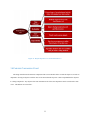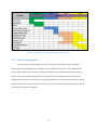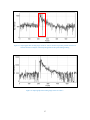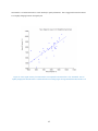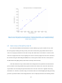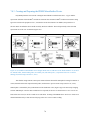
1
BME-DRA-AAG1
NEUROTRACKER 2.0: IMPROVED SOFTWARE FOR NEURAL IMAGING
IN FREELY-MOVING ANIMALS
A Major Qualifying Project Report:
Submitted to the Faculty
Of the
WORCESTER POLYTECHNIC INSTITUTE
In partial fulfillment of the requirements for the
Degree of Bachelor of Science
By
_____________________________________
Justin Hess
_____________________________________
Paul Cupido
_____________________________________
Ellva Feng
Date: May 6, 2014
Approved:
________________________________________
Prof. Dirk R. Albrecht, Major Advisor
1. C. elegans
2. Neural Imaging
3. Freely Moving Animals
________________________________________
Prof. Matthew O. Ward, Co-Advisor
________________________________________
Prof. Joseph B. Duffy, Co-Advisor
1
TABLE OF CONTENTS
Table of Figures ............................................................................................................................................ 4
Table of Tables ............................................................................................................................................. 6
Authorship .................................................................................................................................................... 7
Acknowledgements ....................................................................................................................................... 9
Abstract ....................................................................................................................................................... 10
Chapter 1: Introduction ............................................................................................................................... 11
Chapter 2: Literature Review ...................................................................................................................... 13
2.1
Background ................................................................................................................................. 13
2.1.1
Neuron Structure and Function ........................................................................................... 13
2.1.2
Behavioral Neuroscience .................................................................................................... 16
2.1.3
C. elegans Anatomy and Advantages for Laboratory Use .................................................. 17
2.1.4
The Use of C. elegans in Neuroimaging ............................................................................. 21
2.2 Current Methods and Technology..................................................................................................... 22
2.2.1 Single-Worm Tracking System .................................................................................................. 24
2.2.2 Faumont’s Opto-Mechanical System ......................................................................................... 25
2.2.3 Larsch et al. Microfluidics High throughput System ................................................................. 27
2.3 NeuroTracker 1.0 Function ............................................................................................................... 29
Chapter 3: Project Strategy ......................................................................................................................... 30
3.1
Client Statement and project goals.............................................................................................. 30
3.2
NeuroTracker 1.0 Challenges ..................................................................................................... 31
3.3
Objectives ................................................................................................................................... 32
3.4
Pairwise Comparison Chart ........................................................................................................ 33
3.4.1
Design Function and Pseudocode ....................................................................................... 34
3.5
Design Constraints ...................................................................................................................... 35
3.6
Project Approach ........................................................................................................................ 36
3.6.1
Project Management ........................................................................................................... 36
3.6.2
Financial Management ........................................................................................................ 37
Chapter 4: Alternative Designs ................................................................................................................... 38
4.1
Preliminary Designs .................................................................................................................... 38
4.2
Alternative Designs following Single Worm Tracking Functionality ........................................ 40
4.3
Conceptual Designs and Decisions ............................................................................................. 44
Chapter 5: Final Design .............................................................................................................................. 45
2
5.1
Decisions leading to the Final Design......................................................................................... 45
5.2
Final Design of the ImageJ Macro .............................................................................................. 46
Chapter 6: Discussion of Implementation and Metrics ............................................................................... 53
Analysis of Results ..................................................................................................................... 53
6.1
6.1.1. Single worm study .................................................................................................................... 53
6.1.2
Multiple worm study ........................................................................................................... 58
6.1.3
Comparison Study ............................................................................................................... 61
6.2
Limitations of NeuroTracker 2.0 ................................................................................................ 63
6.3
Applications of NeuroTracker 2.0 .............................................................................................. 64
Chapter 7: A Biological Hypothesis for Design Verification ..................................................................... 65
7.1 Behavioral Variability ....................................................................................................................... 65
7.2 NeuroTracker 2.0: Investigating AIY .............................................................................................. 68
7.3 AIY and Experimental Background .................................................................................................. 68
7.4
Experimental Methods ................................................................................................................ 69
7.4.1 Overview .................................................................................................................................... 69
7.4.2
AIY C. elegans Line Maintenance ...................................................................................... 69
7.4.3
Creating and Preparing the PDMS Microfluidics Device ................................................... 70
7.4.4
Creation of Stimuli and Solutions ....................................................................................... 72
7.4.5
System Set-up ..................................................................................................................... 72
7.5
Results ......................................................................................................................................... 73
7.5.1
7.6
NeuroTracker 2.0 Performance in Conjunction to Experiment .......................................... 73
Experiment Conclusion ............................................................................................................... 73
Chapter 8: Conclusions and Recommendations.......................................................................................... 74
8.1
Conclusions ................................................................................................................................. 74
8.2
Recommendations ....................................................................................................................... 75
References ................................................................................................................................................... 77
Appendix A: Alternative Designs of Code ............................................................................................. 79
Appendix B: User Guide for Final Code ................................................................................................ 83
Appendix C: Detailed Protocol for Preparing and Running an Investigative Experiment with Professor
Albrecht’s Neurotracker 1.0 System ....................................................................................................... 88
3
TABLE OF FIGURES
Figure 1: A detailed diagram of neuron structure (Neuron, 2008). .............................................................................14
Figure 2: Voltage-gated ion channels open in response to changes in membrane voltage. Once activated, these
channels become inactive for a brief period of time and will not open until the original charge is reestablished
(Rye et al, 2013)..................................................................................................................................................16
Figure 3: The structural organization of neural ganglia in C. elegans (Hobert, 2010). ...............................................19
Figure 4: C. elegans life cycle at 22oC. Fertilization in this diagram occurred at the start of the cycle. The blue
hours indicate the period of time it takes for a nematode to advance to the next stage. The length of each
animal is labeled in micrometers. .......................................................................................................................19
Figure 5: Anatomical breakdown of C. elegans involving their locomotion (Altun, 2012). .......................................20
Figure 6: Worm Tracker 2.0 hardware. A small camera (B) is attached to the system below the petri dish (A), with a
red LED bulb (D) facing down on the petri dish (Yemini, 2011). ......................................................................25
Figure 7: Schematic of Faumont’s tracking system (Faumont, 2011). ........................................................................26
Figure 8: Wide-field imaging of neural activity with precise microfluidic chemical stimulation system set-up (Larsch
et al., 2013). ........................................................................................................................................................28
Figure 9: PDMS microfluidics arena which houses multiple worms for behavioral analysis. A stimulus is seen
applied evenly distributed across the arena (right). Arena is pictured from 2.5X magnification. .......................28
Figure 10: The function and means by which NeuroTracker 1.0 collects neuron fluorescence intensity ....................30
Figure 11: Project Objective Tree for NeuroTracker 2.0 .............................................................................................33
Figure 12: NeuroTracker 2.0 pseudocode design structure. ........................................................................................35
Figure 13: Gantt Chart for creating NeuroTracker 2.0 and testing it ...........................................................................37
Figure 14: NeuroTracker button in ImageJ menu bar, designed for quick “one-click” running of the script created by
the group. Highlighted in red. .............................................................................................................................46
Figure 15: A final algorithm design for NeuroTracker 2.0 ..........................................................................................47
Figure 16: Branch information results table from AnalyzeSkeleton for a single worm in a slice. ..............................49
Figure 17: Particle analysis tracking of a single worm using distance formula method. .............................................55
Figure 18: Output graph after tracking single worm for video 1. ................................................................................55
Figure 19: Output graph after tracking single worm for video 2. ................................................................................56
Figure 20: Output graph after tracking single worm for video 3. Red box represents likely behavior of worm coiling
up in ball and collision of skeleton .....................................................................................................................56
Figure 21: Output graph after tracking single worm for video 4. Red box represents possible decreases in
fluorescence due to analysis of the body and gut florescence pixels during tracking .........................................57
Figure 22: Output graph after tracking single worm for video 5. ................................................................................57
Figure 23: Particle analysis tracking of multiple worms at once for every slice in a video. ........................................59
Figure 24: NeuroTracker 2.0 analyzed multiple worm study graphs. Three worms analyzed in each video, one box
represents a different video correlating to Table 3..............................................................................................60
Figure 25: Trace signal accuracy for NeuroTracker 2.0 compared to NeuroTracker 1.0 for 40 animals. Line of
equality displays that NeuroTracker 2.0 functions better for tracking single moving animals than NeuroTracker
2.0 .......................................................................................................................................................................62
Figure 26: Trace signal accuracy for NeuroTracker 2.0 compared to NeuroTracker 1.0 for 18 multiple paralyzed
animals. The line of equality shows that NeuroTracker 1.0 and NeuroTracker 2.0 behave similarly for tracking
multiple paralyzed animals. ................................................................................................................................63
Figure 27: Comparing AWA neural activity to a repeated applied stimulus, prompting the question of how AIY
neural activity correlates to behavior. .................................................................................................................66
Figure 28: A functional map of neurons controlling locomotory behavior in C. elegans (Tsalik and Hobert, 2003). .67
Figure 29: AIY preliminary data for paralyzed animals. Mean fluorescence traces for 3 peak categories (a). Note the
varying neural response to stimuli across animals and trials (b, c). Fraction of response in each category (d). 67
4
Figure 30: (a-d) Different microfluidic device designs. Black lines are indicative of the fluidic channels. A, B, and C
are stimulus inlets; animal loading inlets; an outflow port; and control ports. (e) Operation of device via stream
shifting (f-h) Fluid setup (Larsch et al., 2013). ...................................................................................................70
Figure 31: Wide-field Imaging set-up. (A) Schematic of the arena, camera, and solutions reservoirs. (B) Example of
imaged animals. White denotes microposts. (C-D) Camera images of an animal expressing GCaMP2.2b in
AWA Neurons. AIY animals were imaged in a similar manner (Larsch et al., 2013). .......................................71
5
TABLE OF TABLES
Table 1: Pair-wise Comparison Chart for NeuroTracker 2.0 .......................................................................................34
Table 2: Comparison of NeuroTracker 1.0 to NeuroTracker 2.0 versions of code for a single moving animal ..........54
Table 3: Comparison of NeuroTracker 1.0 to NeuroTracker 2.0 versions of code for multiple paralyzed animals. ...59
Table 4: Comparison of NeuroTracker 1.0 to NeuroTracker 2.0 of average user interventions and average time
tracking each animal ...........................................................................................................................................61
6
AUTHORSHIP
i. Abstract…………………………………………………………………………………………………..........JH, PC
1. Introduction……………………………………………………………………………………………….JH, PC, EF
2. Background and Literature Review…………………………………………………………………………...JH, PC
2.1. Background……………………………………………………….……..........................................JH, PC
2.1.1. Neuron Structure and Function……………………….……..........................................JH, PC
2.1.2. Behavioral Neuroscience………………………….……................................................JH, PC
2.1.3. C. elegans Anatomy and Advantages for Laboratory Use……………….….................JH, PC
2.1.4. The Use of C. elegans in the Laboratory and Neuroscience…………….......................JH, PC
2.2. Current Methods and Technology………………………..….…….................................................JH, PC
2.2.1. Worm Tracker 2.0……………………….…….....................................................................JH
2.2.2. Faumont’s Opto-Mechanical System……………….............................................................JH
2.3. Example of a Neuronal Disease.………………………..….……....................................................JH, PC
3. Project Strategy…………………………………………………………………………………………...JH, PC, EF
3.1. Initial Client Statement………………………………………………......................................JH, PC, EF
3.2. Revised Client Statement………………………………………………..........................................JH, PC
3.3. Objectives………………………………………………..........................................................JH, PC, EF
3.3.1. Design Function and Pseudocode……………….………….................................................JH
The Pseudocode was written by Justin Hess, Pseudocode diagram created by Paul Cupido.
3.4. Design Constraints……………………………………………….............................................JH, PC, EF
3.5. Project Approach………………………………………………......................................................JH, EF
3.5.1. Project Management………………………………………………................................PC, EF
3.5.2. Financial Management………………………………………......................................JH, EF
4. Alternative Designs …………………………………………………………………………………………..JH, PC
The original designs of the code were written by Justin Hess and Paul Cupido.
4.1. Preliminary Designs ……………………………………………………………….……...……....JH, PC
4.2. Alternative Designs Following Single Worm Tracking Functionality……………………...……..JH, PC
4.3. Conceptual Designs and Decisions…………………………………………………………….…..JH, PC
5. A Biological Hypothesis for Design Verification…………………………………………………...…....JH, PC, EF
The experiments were performed with the help of Paul Cupido, Justin Hess, Ellva Feng.
5.1. NeuroTracker 2.0 Restatement of Objectives………………………………………………………….PC
7
5.2. AIY and Experimental Background…………………………………………………………………....PC
5.3. Experimental Methods………………………………………………………………………………....PC
5.3.1. Overview…………………………………………………………………………………....PC
5.3.2. AIY C. elegans Line Maintenance……………………………………………….…….PC, EF
5.3.3. Creating and Preparing the PDMS Microfluidics Device…………………………JH, PC, EF
5.3.4. Creation of Stimuli and Solutions…………………………………………………...…PC, EF
5.3.5. System Set-up………………………………………………………………...……...……..PC
5.4. Results………………………………………….……………………………………………………....PC
6. Discussion of Implementation and Metrics…………………………………………………………………...JH, PC
The testing of the code and analysis of the data was performed by Justin Hess and Paul Cupido.
The testing of code and production of the result graphs was performed by Justin Hess.
The MATLAB data analysis of graphs was performed by Paul Cupido.
6.1. Analysis of Results………………………………………………………………………………...JH, PC
6.1.1. Single Worm Study………………………………………………………………..…...JH, PC
6.1.2. Multiple Worm Study……………………………………………………………...…...JH, PC
6.2. Limitations of NeuroTracker 2.0………………………………………………………………......JH, PC
6.3. Applications of NeuroTracker 2.0……………………………………………………….......................JH
7. Final Design and Validation…………………………………………………………………………………..JH, PC
The final version of the code was written by Justin Hess and Paul Cupido.
7.1. Decisions leading to the Final Design…………………………………………………………......JH, PC
7.2. Final Design of the ImageJ Macro………………………………………………………………...JH, PC
8. Conclusion and Future Recommendations……………………………………………………………………JH, PC
8
ACKNOWLEDGEMENTS
The project team would like to thank the Worcester Polytechnic Institute and their Biomedical Engineering
department for providing the resources and facilities needed to complete this project. We would like to specifically
acknowledge Professor Dirk Albrecht for being a superb advisor throughout the year and for providing us with the
proper guidance needed to overcome each new challenge we faced during the course of the project. We also want to
thank Ross Lagoy in Professor Albrecht’s lab for taking the time to train each of our group members in the
experimentation methods. We really appreciated him teaching us everything about the C. elegans laboratory in order
for us to learn how to operate the neural imaging system independently. We want to thank our co-advisor Professor
Matt Ward for advising the team on the programming aspects of the project when we began writing code for
NeuroTracker 2.0. We also want to thank our other co-advisor Professor Joseph Duffy for the additional advising
during the project for the Biology/Biotechnology department segments.
9
ABSTRACT
In the field of behavioral neuroscience, a need exists for an automated method of tracking neuronal activity in model
organisms with rapid high-throughput screening. Current imaging methods are designed to only examine a single
animal at a time, limiting the understanding of the range and variability of response to stimuli. A wide-field imaged
microfluidics system, designed for examining multiple animals can eliminate this problem. However, the bottleneck
now shifts from the experiment to the data analysis as neural experiments become accelerated by 100 fold. The
current software used for data analysis requires intense user supervision as moving neurons exhibit brief patterns of
ambiguity. We here present NeuroTracker 2.0, an improved software package used to automatically track neuronal
activity in Caenorhabditis elegans and then utilize the software to examine the role of the AIY neuron in its nervous
system.
10
CHAPTER 1: INTRODUCTION
The adult human brain consists of over 100 billion electrically excitable cells. These cells share over 100
trillion different connections between each other, making the human brain one of the greatest mysteries and
challenges in the field of medical science (Wang, 2003). The brain, spinal cord, and these conductive cells called
neurons, are the fundamental components of the nervous system. The brain is at the center of the nervous system and
is responsible for coordinating voluntary and involuntary actions between the other tissues of the body. Neurons are
liable for sending and receiving the electrical and chemical signals needed for this coordination. Networks of
neurons are called neural circuits, and they transduce and integrate sensory input signals to drive many behavioral
outputs such as muscle actions and decision making. Unfortunately, malfunctioning neural circuitry can lead to
behavioral output specific to neurological disease and disorder. Neural circuits are extremely difficult to understand
due to the complexity and vast amount of connections that exist between adjacent neurons. If the neural circuitry
within the human body can be mapped in detail and specific components can be correlated to behavior, possible
solutions to neurological malfunction can be sought after with great efficiency. A need exists for efficient
quantitative neural analysis systems that are designed to understand how neuronal circuits process the information
that governs behavior.
Currently, the complexity of the brain leads to difficult diagnosis and treatment of neurological disorders.
In a study performed across 30 European countries, it was found that in a typical year, about 165 million people, or
38% of the total population have fully developed mental illnesses (H. U. Wittchen et al., 2011). Neurological
malfunction is a pressing issue worldwide as schizophrenia, autism, Parkinson’s disease, Alzheimer’s disease,
epilepsy, depression, and traumatic brain injury continue to inflict suffering on patients and families. Alzheimer’s
disease alone affects 5.2 million people in America (Latest Facts and Figures Report, 2013). This disease is fatal as
the human brain slowly disintegrates and memory loss occurs through the severing and degeneration of interneuron
connections (West Virginia, 2011). It is estimated that 1 out of 88 children before the age of eight will develop
Autism Spectral Disorder (ASD) (Autism Fact Sheet, 2013). The estimated cost for caring for every person with
autism is $35 billion per year. It is estimated that it costs $91 billion annually to care for all Alzheimer’s patients
(Ganz, 2006).
11
With neurological disease a costly and prominent issue in medicine, difficulty in research exists as the use
of human subjects conflicts with many different human rights laws. Researchers turn to a variety of other living
organisms for obtaining knowledge about the brain. One species of animal that is a popular choice for behavioral
neuroscience research is Caenorhabditis elegans (C. elegans). C. elegans are a species of microscopic round worm
that only contain 302 neurons in their neurological system (Hobert, 2010). Surprisingly, they are very relatable to
human beings. All connections of the C. elegans neural network have been mapped out, making this animal a
tremendously advantageous learning tool. Due to their small size, the C. elegans anatomy can be considered
invariable from one animal to another. C. elegans are also inexpensive and widely available to obtain for laboratory
use. Various neuronal staining and neuroimaging techniques can be applied to this organism in order to rapidly
advance our knowledge of neuroscience in both humans and invertebrates. By isolating a particular neural circuit of
interest and probing the circuit with a chemical stimulus, a great amount of knowledge can be obtained from this
animal. However, neuroimaging tools that can accurately identify the neural signaling pathways behind behavioral
response in C. elegans do not function on a large scale. Current technologies can only analyze the neural function of
one animal at a time. Since most behaviors and neuronal responses are variable across individual animals, hundreds
to thousands of trials may be necessary to understand the probability and complete range of responses (Larsch et al.,
2013).
A microfluidic system presented by Larsch et al., can scale-up behavioral neuroscience experiments
involving C. elegans by using wide-field fluorescence imaging described in detail later on in this report (Larsch et
al., 2013). This system can analyze approximately 20 animals at a time. However, this increase in data collection
shifts the bottleneck from the experiment to the data analysis. Data analysis is typically performed using a Javabased image processing program called “ImageJ”, developed at the National Institutes of Health (Schneider, 2012).
A custom script titled NeuroTracker 1.0 collects recorded neural fluorescence intensity data from genetically
encoded calcium indicators expressed at a neuron of interest. NeuroTracker 1.0 has many limitations due to the
large amount of data this system generates. The custom script requires tremendous user supervision across large
data sets as a neuron’s position is often lost due to moments of ambiguity in a recording.
We here present NeuroTracker 2.0, an updated version of NeuroTracker 1.0, which eliminates time
consuming user adjustments. The midline of the invariable, non-ambiguous worm body is used to predict the
12
location of a neuron during these moments of ambiguity. This enables NeuroTracker 2.0 to be completely
automated. This report will first describe the necessary background the team learned in order to create this design.
The project’s plan will be presented in order to display the strategy involved in creating NeuroTracker 2.0. The
different designs explored will be examined before the final design is described in detail. Finally we present our
testing results and conclusions.
CHAPTER 2: LITERATURE REVIEW
2.1 BACKGROUND
In order to create this innovative design, it is important to have a strong foundation of background
knowledge pertaining to neuroscience. Neuron function, behavioral neuroscience, C. elegans anatomy, and modern
neuroimaging methods are all relevant topics that were of great value to the team. The objective of this chapter is to
provide an in depth foundation for each of these subjects and to establish a standard stemming from what can be
currently achieved in the lab using the original NeuroTracker 1.0 system that is planned to be expanded upon.
2.1.1 Neuron Structure and Function
Electrical energy and chemical impulses are essential for cellular process communication within
organisms. The basic unit of this communication is the neuron. A neuron is an electrically excitable cell that
receives and transmits information for orchestrating the functions of the body. Neurons are the core components of
the central nervous system (CNS), which includes the brain and spinal cord regions. A subset of the CNS is the
peripheral nervous system. This contains all ganglia and connections that lie outside of the brain and spinal cord
sectors.
The two fundamental types of neurons that exist are sensory and motor neurons. Sensory neurons respond
to touch, sound, light and a variety of other stimuli. These neurons modulate sensory organs and send signals to the
spinal cord and brain. Motor neurons are responsible for generating cellular action within the body. They receive
signals from the brain and spinal cord and have the ability to create muscular contractions. Interneurons are cells that
connect neurons together to provide signal pathways throughout all regions of the body.
13
Typical neuron structural components consist of a soma, an axon, and dendrites. Figure 1 depicts neuron
components in more detail. The soma is the center body of the cell from which the other two components derive
from. An axon is a special cellular extension that arises from the cell body at a site called the axon hillock and can
reach lengths as far as 1 meter in humans. The role of the axon is to carry a neurological signal to the other end of
the cell and convey that message to another neuron muscle or gland. Dendrites are finger-like structures that
protrude from the cell body and receive information from the axon via electrochemical signals.
Figure 1: A detailed diagram of neuron structure (Neuron, 2008).
14
To help understand how neurons send and receive information about the nervous system, afferent and
efferent neurons are referenced in order to describe the direction of the travelling neural signal. Afferent neurons
convey information from tissues and organs into the central nervous system. Efferent neurons transmit signals from
the central nervous system to the effector cells. Once a signal is delivered to the central nervous system via afferent
neurons regarding sensations experienced on or within the body, efferent neurons will help transmit signals
responsible for behavioral response. These signals include stimuli such as visual stimuli, pain, or pressure.
A voltage gradient is maintained across neuronal membranes by utilizing metabolically driven ion pumps
and gated channels as shown in Figure 2. These pumps and channels are embedded in the neuronal membranes and
coordinate to generate intracellular and extracellular ion concentrations between the signaling chemicals of sodium,
potassium, chloride, and calcium. When a neuron is not sending or receiving signals, the sodium potassium pumps,
using energy from ATP, actively transport sodium ions out of the cell and potassium ions in. This creates a negative
charge inside of the cell relative to the outside. An impulse from a stimulus creates an action potential or a
momentary change in electrical charge that occurs across the membrane. Gated sodium channels open and let
sodium ions flood into the cell, making the inside of the cell positively charged. The reversal of charge causes the
sodium channels to close and gated potassium channels to open, releasing potassium ions out of the cell. The
original charge difference is restored. This is how a signal is carried through an axon to other neurons. When this
inter-body communication system malfunctions, the result is unusual neurobehavioral that is representative of
neurological disease.
15
Figure 2: Voltage-gated ion channels open in response to changes in membrane voltage. Once activated, these
channels become inactive for a brief period of time and will not open until the original charge is reestablished (Rye
et al, 2013).
2.1.2 Behavioral Neuroscience
Behavioral neuroscience is the study of physiological, genetic, and developmental mechanisms involving
behavior in all organisms. This topic includes the studies of nerves, neurotransmitters, brain circuitry, and the basic
biological processes that underlie behavior. It is common practice for experiments of behavioral neuroscience to be
performed on non-human animal models to understand human pathology as many animals are relatable to human
construction. The majority of research in this field focuses on the mental process aspects and the behaviors that
correlate to it. Examples of some thoroughly researched behaviors include sensation, perception, and motivated
behavior such as hunger, thirst, sex, control of movement, learning, memory, and emotions.
The field of behavioral neuroscience aims to understand how neural circuits direct animal responses to
sensory stimuli and how genes and modulating neurons regulate and change their respective behavior. This
interdisciplinary area encompasses the neuroscience, psychology, behavioral psychology and biopsychology.
Scientists in this field can map neural networks from investigative discoveries that pinpoint specific interneuron
activity to a response stimulus. The field of behavioral neuroscience also can provide insight for how neurological
diseases are attributed to specific neurons in the brain and result in respective behavior patterns representative of
neuronal damage/degeneration.
16
This project utilizes an animal model as a tool to further explore neural networks that may exist in human
beings. The animal model used are C. elegans, thus it is important to understand their behavioral neuroscience
aspects.
C. elegans possess sensory neurons that are affected by different olfactory cues that can highlight distinct
behaviors such as attraction, avoidance, feeding, or mating. A C. elegans worm can detect chemical stimuli using a
small number of chemosensory neurons whose morphology and synaptic connections were discovered through
reconstruction of the whole nervous system from serial electron micrographs (Troemel, 1997). There are 11 pairs of
chemosensory neurons found within the bilateral, symmetric and amphid chemosensory organs. These networks
include three pairs of neurons with branched, extended sensory cilia called AWA, AWB, and AWC that detect these
olfactory cues, discriminate among them, and relay this information to the rest of the nervous system for appropriate
response (Troemel, 1997).
In humans, studies show that there is a neural system for evaluating general uncertainty (Hsu, 2005). The
orbital cortex (OFC) is a prefrontal cortex region in the frontal lobes of the brain which is involved in the cognitive
processing of decision-making. It is proposed that the OFC is involved in sensory integration, representing the
affective value of reinforces, and in expectoration. The amygdala is an almond-shaped group of nuclei located deep
and medially within the temporal lobes of the brain in complex vertebrates. It is found that the amygdala performs a
primary role in the processing of memory and emotional reactions. Both the amygdala and OFC are known to
receive rapid, multimodal sensory input. They are also bidirectionally connected and are known to function together
for evaluating the value of stimuli; and both are likely involved in detecting salient and relevant stimuli of uncertain
value. Such a function also provides a reward-related signal that can motivate behavior, by virtue of the known
connections between the amygdala/OFC and the striatum (Hsu, 2005). It is important to understand as much as we
can about neural networks and their relation to specific behavior in order to eventually design treatment for neural
ailments.
2.1.3 C. elegans Anatomy and Advantages for Laboratory Use
Caenorhabditis elegans (C. elegans) are a species of microscopic roundworms, more commonly known as
nematodes, which exist in temperate soil habitats around the world. They normally feed on microbes such as
bacteria and can be isolated from rotten vegetation. C. elegans average about 1 mm in length and are Eukaryotic
17
organisms that have been gaining popularity in research laboratories ever since Sydney Brenner selected them as a
promising model system for his studies in exploring the nervous system in 1965 (Wood, 1988). Brenner selected
these animals due to their anatomical simplicity, ease to grow in bulk, storage capabilities and relativity to human
beings. Due to such small size, C. elegans anatomy can be considered invariable from one animal to another. C.
elegans are widely available and inexpensive to obtain for laboratory use. They reproduce quickly and can be
cryogenically frozen while remaining viable after long-term storage until they are thawed. This animal model is
easily maintainable in a petri dish environment. The typical C. elegans worm nervous system consists of 302
neurons. The first larval stage of the worm has 222 neurons and another 80 develop throughout the typical life cycle
of the worm. The neural organization within the animal is pictured in Figure 3. C. elegans provide a “simple” model
of a nervous system which makes it very easy to track and map the neuronal activity of every connection between
neurons in C. elegans. The neurons in a C. elegans worm are organized in several ganglia in the head and tail and
into a spinal cord-like ventral nerve cord. Each neuron, however, has the capacity to perform complex signal
transduction pathways. Research studies focusing on transcription have shown that a single sensory neuron alone
can express 14 different neurotransmitter receptors and 10 neuropeptides (Etchberger et al., 2007). The C. elegans
nervous system is extensive in both function and cell differentiation, that to which it can represent a great model for
investigating how a human nervous system works. All synaptic connections made by each of the 302 neurons of the
animal are known. This is the only animal for which the entire "neural circuitry diagram" has been determined and
further makes C. elegans an excellent model for study of neurodevelopment.
This animal also offers several novel molecular biological techniques to scientists that only exist for C.
elegans experimentation and are not available for applying to higher eukaryotes. For example, manipulation of the
genome by adding, removing, or altering specific genes occurs by relatively routine procedures in C. elegans,
making the construction of diseased animal models time efficient (Revyakin, 2002). About 35% of C. elegans genes
have human homologs (Revyakin, 2012). A homolog is a sequence of protein or Deoxyribonucleic Acid (DNA) that
shares common ancestry and is therefore similar to another segment. Supporting this claim, it has been shown
repeatedly that human genes when inserted genetically into C. elegans replace their homologs.
18
Figure 3: The structural organization of neural ganglia in C. elegans (Hobert, 2010).
The overall life span of C. elegans is two-three weeks as the animal will grow through a life cycle
containing embryonic development, a four molt larva stage, and an adult stage (Figure 4). The short life cycle is one
advantage of working with C. elegans as a model system. C. elegans development is characterized better than any
multicellular organism, making the worm attractive for cell differentiation analysis. The complete cell lineage, or a
description of all the cell divisions that occur to generate a specific group of differentiated cells of the animal, have
been recorded. The developmental pattern of each somatic cell is known, from the zygote to the adult worm. Thus, a
scientist can identify any cell at any point in development, and know the fate of that particular cell (Revyakin,
2002). It is important to note that the life cycle is temperature-dependent. C. elegans goes through a reproductive
life cycle (egg to egg-laying parent) in 5.5 days at 15 degrees Celsius, 3.5 days at 20 degrees Celsius, and 2.5 days at
25 degrees Celsius (Revyakin, 2002). When these animals reach adulthood, they can produce approximately 300
progeny each. A full grown adult exhibits the anatomical structure shown in Figure 5.
Figure 4: C. elegans life cycle at 22oC. Fertilization in this diagram occurred at the start of the cycle. The blue
hours indicate the period of time it takes for a nematode to advance to the next stage. The length of each animal
is labeled in micrometers.
19
Understanding the anatomy of C. elegans is important in neuroimaging as the fluorescence indicator used
to produce a quantifiable signal often appears throughout the intestinal tract of the worm. The worm body is
cylindrical and encapsulated by a protein cuticle and an epithelial cell layer. The outer layer of the body is
transparent which makes it highly suitable for imaging techniques as all 959 of its somatic cells are visible with a
microscope. The major nerves extend along the ventral and dorsal midline, and a four row arrangement of wall
muscle cells exist on the ventral and dorsal sides. These animals do not have a circulatory or skeletal system. The
hydrostatic pressure that exists internally in C. elegans acts as a “hydrostatic skeleton” and allows for movement
through muscle contraction (Hutter, 2008). Muscle contraction happens from one side to the other and results in a
sinusoidal wave progressive motion. The muscle anatomy provides valuable information that allows for the project
to disregard design for neurotracking in rotating C. elegans circumstances, as the animal’s locomotive structure
keeps movement level.
Figure 5: Anatomical breakdown of C. elegans involving their locomotion (Altun, 2012).
20
2.1.4 The Use of C. elegans in Neuroimaging
The use of C. elegans serves as an important model organism in many different labs. Around the world
many scientists are working full time investigating the biology of C. elegans. Between October 1994 and January
1995, 73 scientific articles pertaining to C. elegans appeared in international science journals. Currently
international laboratory conglomerates are collaborating to sequence the entire 100 million bases of DNA of the C.
elegans genome. In just the short time span this animal has been used to explore neuroscience, it has already led to
seminal discoveries in signal development, signal transduction, cell death, aging, and RNA interference (Aschner,
2008). Many of the basic physiological processes and stress responses that are observed in more complex organisms,
such as humans, are conserved in C. elegans. Not only are C. elegans very relatable to more vastly complex
organisms in basic biological processes, but they also have similar genetic lineages as well. C. elegans homologues
have been identified for 60–80% of human genes, and roughly 12 out of 17 known signal transduction pathways are
conserved in both C. elegans and humans (Aschner, 2008).
Neuroimaging is the use of various techniques to either directly or indirectly image the structure and
function of the brain. The reason that humans are so interested in the brain imaging technique is that humans have a
very good visual system; in fact it is our strongest organ, our most powerful way to understand the world. We
believe that if we can see something we will be able to understand it. Neuroimaging is widely used in the clinical
field to study diseases like Autism. Over the past 40 years, the explosion of neuroimaging technology has enabled
the non-invasive study of the brain in individuals with autistic-spectrum disorder. There are two main categories of
neuroimaging including structural imaging and functional imaging.
Structural imaging deals with the structure of the brain and the diagnosis of large scale intracranial disease
such as tumors. Structural magnetic resonance imaging (MRI) was used a lot to image the brain, however, it
received inconsistent results, partly owing to the heterogeneity of the disorder itself, and partly due to the use of
inappropriate control groups and the limitations of region-of –interest techniques. In the last decade, scientists
started clarifying the relationships between neuroanatomical abnormalities and brain-behavior in Autism. According
to results from anatomical imaging, people with Autistic Spectrum Disorder have specific abnormalities in brain
development and anatomy. It is believed that lesions in specific neuroanatomical areas are due to a stroke or brain
tumors and may cause the development of secondary depression. There is a literary review article, (Soares, 1997)
21
that discusses the structural CT and MRI findings in mood disorder patients to examine these specific
neuroanatomical areas. The results showed that mood disorders are associated with the regional structural brain
abnormalities in particular regions involved in mood regulation (Soares, 1997).
Functional imaging is used to diagnose metabolic diseases and lesions on a finer scale such as the imaging
of Alzheimer’s disease and also for neurological and cognitive psychology research and building brain-computer
interfaces. This imaging technique displayed that people have functional differences in brain regions that are
essential to normal social function including cognition. Returning to the Amygdala, which plays a primary role in
the formation and storage of memories associated with emotional events, research indicated that during fear
conditioning, sensory stimuli reach the basolateral complexes of the amygdala. In particular, the sensory stimuli
signals are reaching the lateral nuclei where they form associations with memories of a certain stimuli. Besides the
central role in fear-related processes, the Amygdala plays a significant role in other emotions as well as the
emotional process with cognitive processing. Baas (2004) demonstrated a common pattern of amygdala activation
that exists across emotional studies by combining results across a large number of fMRI and PET emotion studies in
a meta-analysis. The results showed that there was a strong preponderance of left Amygdala activations over the
right Amygdala in functional neuroimaging studies of emotion processing. (Baas, 2004).
Lastly, proton magnetic resonance spectroscopy is used to measure concentrations and ratios of Nacetylastpartate, creatine and phosphocreatine, and choline. This imaging technique suggests that people with
Autistic-Spectrum Disorder have significant abnormalities in prefrontal lobe neuronal integrity, which relates to the
severity of clinical symptoms.
2.2 CURRENT METHODS AND TECHNOLOGY
One current approach used for monitoring neural activity is electrophysiology. This is a technique where
electrical signals released from neurons are directly recorded. Through this method, a diverse array of ionic
conductances have been able to be measured in C. elegans neurons and neuromuscular junctions including those
regulated by nicotinic acetylcholine receptors (Richmond and Jorgensen, 1999), GABA receptors (Richmond and
Jorgensen, 1999), glutamate receptors (Brockie et al.,2001), voltage-gated calcium channels (Lee et al., 1997), and
mechanosensory transduction channels (O'Hagan et al., 2005). This method presents a lot of difficulties that have to
22
be overcome however when applied to C. elegans. The first challenge with using this method relates to the C.
elegans anatomy. The nematode has a hydrostatic skeleton that is covered by a tough proteinaceous membrane that
holds a highly pressurized internal fluid. This cuticle barrier requires careful dissection in order to properly disrupt
the hydroskeleton and insert it correctly (Shafer, 2006). By disrupting the hydroskeleton of the animal, electrical
recording of neuronal activity in a freely behaving C. elegans is not possible and study of behavioral response is
limited. The size of the C. elegans amplifies this challenge as they are only two-three microns in diameter and
surgical incision of a recording electrode takes a great deal of time per animal and requires a lot of skill.
Optical imaging is a technique used widely amongst C. elegans researchers as it is an invasive method and
uses fluorescent optical indicators. Genetically-encoded calcium probes such as Chameleon or GCaMP are
considered to be the most effective optical indicators used in practice (Schafer, 2004). An active neuron contains a
high presence of calcium as calcium ions generate versatile intracellular signals that control key functions in all
types of neurons. In the presence of calcium, these two fluorescent proteins display an increase in fluorescent
resonance energy that directly relates to neural activity. Calcium indicator imaging presents a few advantages over
other neuroimaging techniques as C. elegans are a transparent organism. No dissection is required in order to
analyze neurological response, enabling a wide range of behavioral response to be studied. Also, the C. elegans
nervous system is compact and discernible compared to other organisms, making it possible for activity in multiple
neurons to be measured simultaneously. This feature makes it possible to identify temporal correlations between the
neural circuitry that can provide even greater insight to the mechanisms of neurological function than by just
viewing a single neuron at once (Schafer, 2006). The major disadvantage to this technique is that calcium indicators
are a one-dimensional analysis tool. They can only provide one type of information output and cannot measure
individual ionic conductance or detect subthreshold changes in cell membrane potential.
A final technique used for neuroimaging in C. elegans is in vitro physiological analysis. In order to
compile information about ionic conductance and the manner about which they depend on gene products, C. elegans
ion receptors and channels are often expressed in heterologous Xenopus oocytes (frogs) or fibroblasts with
mammalian derivatives. This cell culture technique makes it possible to compare wild-type and mutant cells
physiological properties in vitro.
23
There are advantages and disadvantages to each method described above. NeuroTracker 2.0 was designed
for optical imaging analysis in C. elegans that were genetically modified to express GCaMP at specific neurons of
interest. Two examples of neuron particle analysis tracking systems using optical imaging are described below for
comparison to the system used for our project.
2.2.1 Single-Worm Tracking System
Worm Tracker 2.0, a single-worm tracking system, was developed by Eviatar Yemini at the University of
Cambridge that proves to be an improvement upon his lab’s original design to track C. elegans (Yemini, 2011). The
hardware includes several features as seen in Figure 6, such as a small attachable camera below the petri dish with a
red LED bulb facing down above the petri dish. This system also uses a similar computational model for analyzing
behavior. It converts all videos of C. elegans into an eight-bit grayscale version, implements a threshold, and
computes the center of the worm as the pixel mean of the x and y value of pixels in the video. One of the biggest
limitations of it however, is that it lacks the functionality to track many freely-moving multiple worms; it can only
sufficiently track a single worm in a given video (Yemini, 2011). This system cannot track neural activity, and can
only track animal behavior.
24
Figure 6: Worm Tracker 2.0 hardware. A small camera (B) is attached to the system below the petri dish (A), with a
red LED bulb (D) facing down on the petri dish (Yemini, 2011).
2.2.2 Faumont’s Opto-Mechanical System
Another tracking system created by Faumont et. al takes advantage of virtual reality to track C. elegans in
real time for understanding their behavior. The tracking system creates virtual environments of the worms through
optogenetic activation of the sensory neurons, and images the activity of neurons in real-time using a high
magnification lens (Faumont, 2011). This system diverts light to activate the neurons in a given worm using a fourquadrant photomultiplier tube (PMT) by means of a beam splitter or a dichroic mirror. This system of circuitry is
25
able to then properly center the fluorescence target of the neuron on the worm while simultaneously recording
behavior and neuronal activity of the worm (see Figure 7) (Faumont, 2011). However, this system can only collect
data from a single animal at a time.
Figure 7: Schematic of Faumont’s tracking system (Faumont, 2011).
26
2.2.3 Larsch et al. Microfluidics High throughput System
NeuroTracker 2.0 is designed for analyzing data collected through a GCaMP optical neuroimaging
technique. The specific system the software is applied to uses a standard inverted epifluorescence microscope was
built on a Zeiss AxioObserver to continuously record more than 20 C. elegans at once automatically (Larsch et al.,
2013). To minimize motion blur and increase signal to noise ratio, the objective magnification (M) is reduced
significantly. Compared to the 40X objective commonly utilized, high numerical aperture (NA) objectives
(2.5x/0.12 NA or 5x/0.25 NA) and a sensitive low-noise electron-multiplying charge coupled device (EM-CCD)
camera greatly increase the signal to noise value of fluorescence signals from the neurons of C. elegans (Larsch et
al., 2013). These components are pictured in Figure 8. This technique results in wide-field recordings of activities in
sensory neurons and interneurons to ease the analysis challenges compared to that in the past.
As shown in Figure 9 below, C. elegans are kept in a PDMS microfluidic arena that is attached to three
stimulus streams for chemical stimuli purpose. Attaching tubing of chemical stimulants and base stimuli to the
microfluidics arena as seen in Figure 8 creates an easy chamber for high-throughput testing purposes. The
microfluidics of the PDMS arena allows for precise stimulation in spatiotemporal patterns of a desired chemical for
evoking neural response. Up to 20 worms can be exposed to precise timing of the same stimulus in order to
understand neural activity in specific neurons being tested correlated to behavior patterns in this arena. The field of
view for a wide-field 2.5X objective lens is demonstrated in Figure 8. Imaging at 2.5X magnification has a better
signal to noise ratio compared to imaging at 40X magnification.
27
Figure 8: Wide-field imaging of neural activity with precise microfluidic chemical stimulation system set-up (Larsch
et al., 2013).
3 mm
Figure 9: PDMS microfluidics arena which houses multiple worms for behavioral analysis. A stimulus is seen
applied evenly distributed across the arena (right). Arena is pictured from 2.5X magnification.
28
2.3 NEUROTRACKER 1.0 FUNCTION
Now that we have explained the system set-up used by the team to collect experimental video recordings,
we can now discuss the software used to analyze these videos. NeuroTracker 1.0 neural activity quantification is
displayed in Figure 10. The raw video in the figure represents exactly what a recorded video would look like for a
single worm in the microfluidics arena. This worm in this demonstration has been genetically modified to express
GCaMP at the sensory neuron AWC through microinjection. As the worm moves about the arena, the concentric red
circles representing the tracker, expand and relocate to the largest area of greatest pixel value for the next frame
(white pixel value = 255). This region of pixel fluorescence intensity relates to neural activity. A very active neuron
contains a greater amount of pixel intensity, represented in red on the heat map in the right half of Figure 10. The
purple arrows in the figure represent the correlation between when stimulation ended, neuron activity was the
greatest, and when reversal locomotion was observed.
Notice the means by which NeuroTracker 1.0 finds the position of the neuron for the next frame. It is
largely based on the size of the largest group of high intensity pixels. This creates major issues that our algorithm
was designed to overcome as NeuroTracker 1.0 is completely dependent upon only tracking a search region with
high fluorescence intensity pixels. This is problematic when a neuron has a low level of brightness. Background
noise and brighter pixels throughout the worm body can also be analyzed incorrectly, thus ruining proper data
analysis.
29
Figure 10: The function and means by which NeuroTracker 1.0 collects neuron fluorescence intensity
CHAPTER 3: PROJECT STRATEGY
The overall goal of this project is to design an automated method of tracking neuronal activity in model
organisms with high-throughput screening. In order to develop such an advanced system, it is significant to
understand the shortcomings of the current software exit in the lab, NeuroTracker 1.0 and then expand our
knowledge on these issues. With the direction of the project advisor, Professor Albrecht of Worcester Polytechnic
Institute in Worcester, MA, our project team determined the following objectives, functions, and constraints for the
design development.
3.1 CLIENT STATEMENT AND PROJECT GOALS
Before starting the design process, the project team gathered information from the recent literature and
many interviews with our client. Based on the needs of our client Professor Albrecht, our project team developed a
client statement.
30
Initial Client Statement: Design, implement, and characterize an automated vision and analysis system to
identify and track multiple freely-moving C. elegans (nematodes) in a microfluidic environment while
simultaneously quantifying neural activity on a large scale.
After researching on the preexisting systems, the project team sought to improve the current worm tracker
system focusing on increasing the number of freely-moving worms and advancing the automated system. The
improved worm tracker NeuroTracker 2.0 would include the best characteristics of pre-existing system, while being
able to reduce the times of user intervention. The following is a list of the overall project objectives, functions, and
constraints.
3.2NEUROTRACKER 1.0 CHALLENGES
NeuroTracker 1.0 is used in the lab to analyze neuronal activity data of the C. elegans worms being
exposed to chemical assays in order for researchers to try to correlate worm behavior with neuronal activity. The
current version of NeuroTracker has the functionality to record both sensory neurons and interneurons that respond
to the chemical assays being experienced by the worms. However, the current version cannot track more than 3
freely-moving worms. This software is also not compatible with dim neurons such as AIB, as it often fails to detect
calcium signals. When tracking multiple worms, NeuroTracker 1.0 is only efficient when used with paralyzed
animals.
NeuroTracker 1.0 has many issues during tracking. One of these is that the variability of the neuron
position possesses a great problem when tracking freely-moving worms with erratic locomotion. Background noise,
including many dust particles in the video, are incorrectly picked up by the expanding search region of the tracker.
The gut of the neuron, including pixels down the worm body, also can be incorrectly analyzed by the tracker as
these regions can exist at higher intensity than the neuron itself. Finally, the biggest issue is that when the neuron
brightness dims after the worm is no longer responding to the stimuli, the neuron pixel region dims in brightness.
This causes the tracker to ultimately lose the location of the neuron, thus requiring the user to constantly be clicking
back on the neuron during tracking. This semi-automated process proves to be extremely tedious for the user, as
31
efficiency is very low. A user intervention is defined as a time when the tracking system halts and requires the user
to adjust its position to continue proper analysis via reselecting on the neuron.
3.3 OBJECTIVES
The project team created a list of objectives below for the client to identify what the exact needs that
NeuroTracker 2.0 should provide. Three main objectives were obtained based on the recent literature and a series of
interviews with our client. Overall, the objectives were created taking into account the many issues in NeuroTracker
1.0.
1. Time efficient
a. Eliminate user interventions so that tracking is fully automated within a reasonable time limit
2. Reliability
a. Ignore background noise
i. Avoid fluorescence pixels in the background of videos
b. Track a weak neural signal
i. Tracker needs to maintain the position of the neuron when pixel brightness is low
c. Maintain signal accuracy
i. The measured change in fluorescence intensity does not lose its accuracy from
NeuroTracker 1.0.
ii. NeuroTracker 1.0 is considered to be very accurate
3. User-Friendly
a. NeuroTracker 2.0 should be simple to use for anybody, no matter what their experience level is.
4. Adjustable
a. Future Image processing algorithms are amendable and are presented to future coders in an
organized manner for promoting other updates to the code.
These objectives are organized into a visual diagram (Figure 11) below.
32
Figure 11: Project Objective Tree for NeuroTracker 2.0
3.4 PAIRWISE COMPARISON CHART
The design team then used a Pairwise comparison chart seen in the table below to rank the objectives in order of
importance. Scoring an objective with the value of one means that the objective is more important than the objective
it is being compared to. Any objective that was determined to be of the same importance can be scored with a value
of 0.5. This did not occur in Table 1.
33
Table 1: Pair-wise Comparison Chart for NeuroTracker 2.0
Objectives
Reliability
Time
Efficient
UserFriendly
Adjustability
Total
Reliability
X
0
1
1
2
Time
Efficient
1
X
1
1
3
UserFriendly
0
0
X
1
1
Adjustability
0
0
0
X
0
The most important objective is time efficiency based on the Pairwise comparison chart. The design system
should be able to process hours of recorded neuron function with more than 20 C. elegans in the system at a time
with minimal user intervention. This by far is the most important design factor for gauging the success of
NeuroTracker 2.0. NeuroTracker 2.0 needs to be reliable otherwise improving time efficiency is pointless. The third
important objective is that the system needs to be user-friendly. Adjustability, being the last ranked objective is still
important even though it received a low score. The other three objectives just take precedence.
3.4.1 Design Function and Pseudocode
After discussing options for the best approach to automating NeuroTracker 1.0, our group proposes the use
of using a medial axis algorithm. A medial axis takes a whole contour of an image and uses an erosion technique to
shrink it down to a single pixel midline.
Shown in Figure 12, a medial axis/erosion algorithm requires four precursor steps: remove background
noise, dilate and remove outliers, skeletonize, and analyze the midline to store coordinates. In order to create a
midline of every animal in a video, it was found that the video must be first converted to binary. In order to do this
the background noise was required to be removed before a binary mask could be applied to the entire video, making
pixel values equal to either zero or one. In order to prevent a midline from being segmented and inaccurately
representing the body of a worm, it was required for the video to undergo numerous dilation procedures which
essentially thickens the body of the animal. Removing outliers erased pixels that did not cluster amongst the worm
bodies, making it so that background particles did not receive the skeletonization (erosion to midline) process.
34
Figure 12: NeuroTracker 2.0 pseudocode design structure.
3.5DESIGN CONSTRAINTS
Following the analysis of the objectives, a list of constraints was generated to assist in defining the overall
design planning. Tracking the neurons in the moving nematodes is one of the biggest constraints in this project.
With multiple nematodes moving in the microfluidic environment, the system must successfully track the position of
neurons to the corresponding animals. Also, with the increasing number of the freely-moving C. elegans, the
maintenance of the accuracy in the currently used system is another challenge that needed to be concerned in the
later design process. Tracking multiple worms, not just a single worm, simultaneously is a goal as well as a design
35
constraint that needs to be taken in to account. Computational power is another potential issue in the project. The
team could possibly handle 20 anesthetized, paralyzed animals at a single time. It requires the system to create 20
coordinates to track neuron positions in individual subject. The computational system needs to store history of each
frame from each video, which needs the system to spend a lot of processing power in the procedure. It will be
important to make sure the new design of the code does not run slower than the semi-automated process used in the
current NeuroTracker 1.0.
3.6 PROJECT APPROACH
ImageJ is the main program the team uses to perform the current neuronal stimuli evaluation in the lab. As
none of the members in the team have experience in ImageJ in the past, the need to quickly learn the computer
program and especially the study of macro functions is the start of the technical approach to the project. Macros,
written in ImageJ’s macro language that is extremely similar to the C programming language, are simple programs
that automate series of ImageJ commands. Pseudocode, an informal high-level description of the operating principle
of a computer program or other algorithm, will be used thoroughly in the early project procedure to help understand
the existing codes and write future plans such as the adding of skeleton and medial axis to the existing pseudocode.
Once the pseudocode for the future plans are completed, the team will then need to convert the pseudocode into the
script in ImageJ using macro program. The design group will spend two-thirds of the project working on performing
new experiments on recording the neural behavior of C. elegans and gathering the new data for the analysis using
the code. Among all technical ways, the most challenging one is the modification of the existing script and testing
the script with the data sets to ensure they are compatible with each other. Besides the computational design on
coding in ImageJ, the physical design on microfluidic device is the other task in the project after it was discussed
with our advisor.
3.6.1 Project Management
A Gantt chart is shown below in Figure 13 and was used to track the team’s progress in an organized
fashion throughout the entirety of the project.
36
Figure 13: Gantt Chart for creating NeuroTracker 2.0 and testing it
3.6.2 Financial Management
As mentioned in the technical approach, none of the members in the team has ImageJ background.
Learning the functions and applications of ImageJ is the core component in this project. After conducting some
research and discussing with our advisor, we spent $25.00 purchasing a book about Image Processing based on
ImageJ to help us get familiar with this program. For other parts such as performing the new experiment and
designing microfluidic device, the advisor gave our group the permission to use materials such as plastic wells and
instruments such as a Zeiss microscope directly from the lab. This means that part of the funding of the project will
be contributed to the general lab supplies.
37
CHAPTER 4: ALTERNATIVE DESIGNS
4.1 PRELIMINARY DESIGNS
The project design aims to track the location of the neuron in a single moving worm throughout an entire
movie with limited user intervention. To achieve this goal, the team explored preliminary designs such as using the
center of mass, distance formula, and an indexing method.
While running the original script of NeuroTracker 1.0, the central issue with the version was that the
tracking target window moved easily to the background or the gut fluorescence in the animal. This was caused by
the intensity of the fluorescence in the background and gut existing at a higher value than that in the neuron. In order
to prevent the target window from moving out of our specific region of interest, it was decided to create a skeleton
from the worm image. The skeleton version of the worm, as shown in Appendix A, was a result of eroding the worm
body pixels to a center line of the worm and removing the unwanted fluorescence particles in the worm body.
ImageJ presented three functions that were used in order to accomplish this: “Dilate”, “Remove Outliers”, and
“Skeletonize Stack”.
The “Dilate” function is necessary for creating a complete skeleton of the imaged animal. This function
enlarges the pixels of the image and when used in conjunction with the “Remove Outliers” function, creates a
pixelated animal that is more likely not to have any gaps when skeletonized. The “Skeletonize Stack” method is the
function that removes pixels from the largest pixel groupings until a single pixel center line is left remaining. The
entire skeletonization process involves 6 “Dilate” and “Remove Outliers” functions before the “Skeletonization”
function can be called, as seen in the first figure of Appendix A. This is an alternative design that the group decided
that was changed in the final code because the video needed more function calls of the remove outlier procedure.
The original design that used less of these procedures as a result had more dust particles, making it a version of the
code that was improved upon in the final design. It was also not used because when the skeleton is dilated and the
outliers are removed it can shrink the skeleton or elongate it so that the pixel coordinates of the head are off.
In search of a new strategy, the team met up with Professor Ward, a professor of computer science and
bioinformatics and computational biology at Worcester Polytechnic Institute. The team was guided to use the center
of mass of the worm skeleton to track the position of the neuron throughout the entire movie. The center of mass is
38
defined as a point that represents the mean position of the matter in a body or system. Thus, the center of mass is in
the unchangeable location for every worm. Professor Ward also suggested that the team calculates the distance
between the center of mass and the head of the animal to estimate the position of the neuron. The neuron would then
be expected to be a specific percentage away from the head. However, the center of mass was defined differently in
ImageJ terms. The center of mass in ImageJ is the average position of coordinates. Therefore when the worm is
curved or not in a linear position, the center of mass does not exist on the worm skeleton. The system will not be
able to figure out the new head position and it will skew the coordinates of the neuron.
Another preliminary design idea that was experimented with was to prompt the user to select the head and
tail locations on the video, and to match the head and tail coordinates with the saved coordinates from the skeleton
using the “Save XY Coordinates” function from ImageJ. The “Save XY Coordinates” function simply records all
pixels coordinates with a value higher than the background (~255). By using this function and knowing the head
coordinate, the macro would be able to walk down the worm skeleton to the location of the neuron. This method was
found to be unsuccessful as the ImageJ function “Save XY Coordinates” records coordinates in random order and
retrieving the neuron coordinate requires sorting the pixels in the order of from head to tail (see Appendix A).
The team discovered a Java programmed ImageJ plugin called AnalyzeSkeleton, which returns branch
statistics for a skeleton video (Arganda-Carreras, 2010). After meeting with Professor Albrecht, our advisor, the
team considered to edit the AnalyzeSkeleton plugin by programming in Java to just return the skeleton endpoints.
Fortunately, one of the team members was able to obtain coordinates near the head and the tail position on the
skeleton of the worm using Analyze skeleton without having to edit it. To gain this result, for each frame of the
movie, the team copied the image and inserted it into the AnalyzeSkeleton function. This function produces a
window that contained coordinates for the head and tail endpoints (Arganda-Carreras, 2014). To ensure the
coordinates obtained by the system were on the skeleton, the team altered the erosion of skeleton to shrink the worm
a few pixels on the edges.
For every frame in the movie, the system copied the current frame of that image and applied the
skeletonized method to the slide. The system then saved both the head and the tail coordinates. After the analysis of
the whole video, the system sifted through these saved coordinates and prompted the user to identify the head
coordinates by matching them to the stack of images. The team used the distance formula to calculate the distance of
39
the head coordinates in every two successive slides. For instance, the head coordinate of the worm in the first slide
was saved and this coordinate was compare to the head coordinate in the second slide. The team decided that the
relative distance of the two successive head coordinates should be less or equal to 5-10 units (average of the
maximum rate of change we calculated in different trials) by using the distance formula:
Distance = sqrt[ (x2 - x1)2 + (y2 - y1)2 ]
4.2 ALTERNATIVE DESIGNS FOLLOWING SINGLE WORM TRACKING FUNCTIONALITY
One of the first designs used to run the NeuroTracker script was when the user would have to select through
the menus “Plugins→ Macros→ Neurotracker[t]”. This was removed as the “one-click” button surprisingly
improved user friendliness of the program and starting NeuroTracker became less frustrating.
To begin the image analysis process, originally the team used only one specific thresholding applied to
every video. The main problem with this tactic was that during B term our group only tested the video on a select
few single-worm videos. The thresholding was hard-coded and worked for these videos, but once it was C term the
team started to improve the functionality of the code following several problems with this design choice. The main
problem with having a hard-coded threshold was that there is no way it can work universally for every video. Some
videos have different contrasts and confocal lighting to them compared to other videos. As a result, having just one
specific thresholding would not produce an accurate skeletonization version of every different type of video (Figure
A.1). Due to the non-universal functionality of hard-coding the thresholding procedure, we eventually changed the
thresholding to automate the process. Below is what the code looked like before we automated the thresholding
process in Appendix A.
The next necessary coding step needed to change how the data was being extracted and stored from
AnalyzeSkeleton’s Branch Information window. Currently suspect neuron coordinates were being extracted and
inserted into four separate arrays called xcoor1, ycoor1, xcoor2 and ycoor2. This data analysis method proved
inapplicable for tracking multiple worms, as many more arrays will be needed to store data for every individual
worm. The other problem with using arrays when our group had to add the multiple worm tracking functionality was
that having a certain number of arrays has to be hard-coded; in other words, limitations of ImageJ include that the
40
software is unable to create multi-dimensional arrays. Shown in figure A.2 in Appendix A is what the code looked
when we used the array method before we had to resort to using text files to store the data in the final design.
Inside of this “for” loop iterating “i”, the macro then runs through the branch information results table in
another “for” loop. This inner “for” loop that iterates “j” parses the data from the text file that has the results saved
from the branch information results table. This part of the code is very important because it ignores all outlier points
from the skeletonized video that were not eliminated from earlier in the macro using the “Remove Outliers”
command. Without this step, extracting the neuron coordinates later on would still contain outlier points and would
not always get points that are even on the skeleton.
Another design idea that did not work is that our group thought for tracking multiple worms a simple
modification could be added at the end of the outer “for” loop that iterates “i”. First, in the “for” loop that iterates “j,”
after it parses the data and only collects skeletons with branch lengths greater than 10 from column 3 (index 2), it
collects the coordinates 1 and 2 from the table. The macro collects data for coordinate 1 from columns 4 (index 3)
and 5 (index 4); and data for coordinates 2 from columns 7 (index 6) and 8 (index 7). It does this by storing these
values in arrays, which was part of the old design for data analysis purposes to easily track a single worm. This
method, however, does not work for tracking multiple worms. The original version of the macro collects data from
AnalyzeSkeleton and stores the x and y values for each coordinate into the four arrays called x1coor, y1coor
(Coordinate 1), x2coor and y2coor (Coordinate 2) (see figure A.3).
As part of the original design using the four arrays (x1coor, y1coor, x2coor and y2coor) in the form of
coordinates 1 and 2 for one slice, the macro then exits the inner “for” loop to gather the data into larger arrays that
store the head and tail coordinate data for every slice. Our team thought it was necessary to use these four arrays xcoor1, ycoor1, xcoor2 and ycoor2 - because the inner “for” loop’s coordinate variables (x1coor, y1coor, x2coor
and y2coor) are replaced with the new head and tail coordinates for the next slice in the video once the outer “for”
loop finishes analyzing one slice and goes to the next slice. The original version of the macro used xcoor1, ycoor1,
xcoor2 and ycoor2 to store the head and tail coordinates for each slice and will then be manipulated further once the
entire video is analyzed using AnalyzeSkeleton. We thought that outside of the inner “for” loop, we could simply
just store the data from the inner “for” loop into these variables for every slice and change the counter index to be
equal to “i” to collect data for multiple worms but this design idea would not work. Tracking multiple worms is
41
much more complicated than performing a simple change such as that; the only way to avoid hard-coding multiple
arrays to collect data and track multiple worms is to use text files.
One of the original designs of the code that severely reduced efficiency and halted automation of the
analysis process was when the code asked the user which coordinate the head was after the AnalyzeSkeleton process.
After the AnalyzeSkeleton procedure is completed and the outer “for” loop is done analyzing the entire video, the
macro turns to the first slice in the video and asks for user input. The macro would ask if coordinate 1 from the first
slice is the head or not. If it is, then coordinate 1 is stored as the first neuron coordinate (or skeleton head coordinate)
in the neuron x and y coordinate arrays (neuroncoorx and neuroncoory respectively). If the user says “no,” then
coordinate 2 must be the skeleton head and is stored as the first neuron coordinate in the respective arrays (see
Figure A.4).
This original design is not optimal to be used in the final version of the code because it asks for manual user
input during the middle of NeuroTracker 2.0’s procedure. Ideally, we only want the user to intervene once and at the
beginning of the process. That way, the user can run an experiment while they wait for the code to run. This is not
possible with this original design to ask which coordinate is the head. That is why this code is not used in the final
design in order for automated image analysis and particle tracking to occur.
Now that the code from the original design knows which coordinate is the head after asking the user, the
original code would then figure out every skeleton head coordinate for the entire video. The last part of the macro in
the original design would then use a very complicated “for” loop that sorts through xcoor1, ycoor1, xcoor2 and
ycoor2 to only get the head coordinates of the skeleton for every slice of the video (see Figure A.5).
The original code above shows a “for” loop that has to sift through the arrays for coordinates 1 and 2 for
each slice to finally get the head coordinate of the skeleton, which in this case after eroding the original worm
enough is the location of the neuron. The “for” loop starts out checking if the neuron coordinate for the first slice
was from either coordinate 1 or 2 (from user manual input). For every slice, the algorithm then performs several
checks on the neighboring x and y values of the neuron coordinate from the previous slice with coordinates 1 and 2
from the current slice it is analyzing. In particular, it cares mostly if the y coordinates flipped between slices and
how far apart the x coordinates are. A “flip” occurs between y values if the y coordinate 1 is less than the y
coordinate 2 of the current slice and if the y coordinate 1 is greater than the y coordinate 2 from the last slice, or vice
42
versa. This “flip” means that the AnalyzeSkeleton results switched the head coordinate between coordinates 1 and 2
when the worm’s head passed the tail horizontally, or if the tail passed the head horizontally. If the last slice had
coordinate 1 as the neuron coordinate, it checks if the y values flipped between the neuron coordinate from the last
slice and coordinate 1 from the current slice. If so, that means that coordinates 1 and 2 could have switched to be the
head coordinate. If the y values flipped, the macro then checks if the x values are similar between the neuron
coordinate from the last slice and coordinate 1 from the current slice. If so, then that means coordinates 1 and 2 have
flipped and the head coordinate is now coordinate 2 for the current slice, meaning we want to store the coordinate 2
value into the neuron coordinate array for the current slice we are analyzing. However, if the y values flipped and
the x values are far away from each other that means coordinates 1 and 2 did not switch, meaning we want to store
the coordinate 1 value into the neuron coordinate array for the current slice we are analyzing. Finally, if the y values
did not flip between the neuron coordinate from the last slice and coordinate 1 from the current slice then that
obviously means we still want to store coordinate 1 as the neuron coordinate for the current slice we are analyzing.
This is because the AnalyzeSkeleton plugin stores its head and tail coordinates in increasing x value for a slice, and
it is never certain which coordinate is the head by looking at the branch information results (Arganda-Carreras,
2010). However, this “for” loop algorithm will only work to track a single worm; its functionality will not be able to
track multiple worms because it is only able to track two different arrays and checking if the values flip or not. That
is one of the main reasons why this design was not implemented in the final version of NeuroTracker 2.0, as our
team needed to implement the functionality to track multiple worms in the code.
Now that the original code from the macro would have all the coordinates for every neuron for every slice
in a given video, these coordinates could be used as input variables later on in the script to analyze neuronal activity.
By plugging in the arrays neuroncoorx and neuroncoory into the part of the script that makes an oval around the
estimated neuron position, we were originally able to have a more accurate and efficient way of verifying neuron
position during calcium fluorescence analysis than in NeuroTracker 1.0 (see Appendix A).
After testing the modified version of the macro, the particle analysis process worked to automatically track
the neuron position. However, as mentioned previously, the use of solely arrays to store neuron coordinates will
only work to track a single worm. That is why our group moved on from using arrays to text files in the final version
of the code. At the time it was huge improvement, as we were able to obtain better data at a faster rate without
43
tedious user intervention.
As the end result, we were able to completely automate fluorescence collection for the neuron in an entire video
using the original design of the code as described above. There was complete automation of particle analysis with no
user intervention when tracking just a single worm. The target window where the macro collects fluorescence data
would not run down the body of the worm or jumping to background noise for the video of a single worm provided
to us.
4.3 CONCEPTUAL DESIGNS AND DECISIONS
The main challenge of the design is to track the neuron. The ideas of using center of mass, distance formula,
and indices method failed as we mentioned in the preliminary design section and did not give us desired neuron
positions. The idea of center of mass suggested by Professor Ward to get the distance between the head and the
center of mass to track the neuron didn’t work when the worm was curved as the center of mass coordinates were
not located on the skeleton. Another conceptual design of comparing the distance between the head and the neuron
for every two successive frames failed to work since it wasted too much computer processing power. The index
method the team developed to estimate the head position and the center of mass did not succeed due to data ImageJ
saved not being consistent throughout the entire movie.
The final design the team decided to use was implemented because it is feasible, easy to program, and the
neuron tracking target window is guaranteed to be on the skeleton. The final design was able to retrieve the
coordinates of the neuron which are in the head location on the skeleton. After using the AnalyzeSkeleton plugin
and the particle tracking function that sifts through both coordinate 1 and coordinate 2 without outliers we were able
to get the neuron coordinates. The last alternative design completed in the fall during the project was able to track
the neuron successfully on the skeleton of a single moving worm.
44
CHAPTER 5: FINAL DESIGN
5.1DECISIONS LEADING TO THE FINAL DESIGN
Many of the design choices that our group took to come up with the final version of NeuroTracker 2.0
focused on several factors. One of the most important factors was user intervention, as we wanted to make the
analysis of the data process as automatic as possible with the least amount of user intervention. More specifically, it
is desired that the user only would have to intervene once at the beginning of running the program in ImageJ.
Despite how long the analysis process takes to run, it is most beneficial for efficiency if the user only has to start the
program without the inconvenience of waiting to have to intervene again in later steps of the analysis process. Both
NeuroTracker 1.0 and the team’s alternative designs required the user to not just give input to the program multiple
times, but also have to manually intervene much later in the analysis process. This involved making sure the oval
that was tracking the neuron coordinates being analyzed would always stay on the neuron, by clicking many times
on the neuron when the oval lost track or fell off the neuron. The final design of NeuroTracker 2.0 solves this
problem by increasing efficiency dramatically by requiring only the user to click on the neuron(s) once at the very
beginning of running NeuroTracker 2.0. This allows the user to start the program and walk away unattended to run
experiments or perform other activities that could not have originally been performed when having to tediously
intervene in the analysis of data using the original NeuroTracker 1.0.
Another vast improvement in the final design of the code in NeuroTracker 2.0 involves the ability to track
multiple worms at once automatically. There was a considerable amount of coding that had to be added just for this
functionality, as the process becomes much more complicated when tracking the movement of multiple neurons at
once and analyzing their activities collectively. In NeuroTracker 1.0, not only would the user have to painstakingly,
manually help track the positions of the ovals staying on and analyzing the neurons, but they also would have to
perform the entire analysis process again for each different worm. This makes the analysis to take considerably
longer than tracking a single worm and is overall inefficient. The final design of NeuroTracker 2.0 helps alleviate
this process by trying to track multiple neurons at once. As a result, the analysis process is able to collect activity of
every neuron for every frame/slice in a video data set being analyzed when the worms are not touching and their full
bodies are showing. Overall, the final design improves not only the accuracy of the analysis by creating less noise in
45
the output data of neural activity but it also improves efficiency considerably by having the least possible amount of
user intervention.
5.2 FINAL DESIGN OF THE IMAGEJ MACRO
The additions to NeuroTracker 1.0 involved some pieces from the preliminary designs while many of the main
ideas of preliminary designs were removed in the final design process. A simplistic yet time saving addition to the
program that found its place in the final design was a Neurotracker button on the main menu bar in ImageJ (Figure
14).
Figure 14: NeuroTracker button in ImageJ menu bar, designed for quick “one-click” running of the script created by
the group. Highlighted in red.
In order to originally run the NeuroTracker script, the user would have to select through the menus
“Plugins→ Macros→ Neurotracker[t]”. By removing even just this three step menu navigation process, the “oneclick” button surprisingly improved user friendliness of the program helping to meet this specific design objective.
The first part of the code as mentioned in the last section is the only part of the analysis process in
NeuroTracker 2.0 that requires manual user intervention. This specifically is when the code asks the user to select
the neuron(s) on the video. Once the user is finished selecting the neuron(s) they have to simply press the spacebar.
This process is implemented through the use of a while loop: nothing happens unless the user clicks on at least one
neuron and presses the spacebar. The code will not proceed until the user lets the code know where the neuron(s) are
that need to be tracked.
46
Once the user has pressed the spacebar and clicked on every neuron in the video, the log will print how
many neurons have been recorded, enhancing ease of use. The code stores the x and y neuron coordinates in two
separate arrays called xmancoor and ymancoor. The code also trims the two arrays to only contain any real x and y
coordinates of the neurons and eliminates all (0,0) coordinates to help later parts of the code to work, and finally
prints the arrays to the log so the user can verify those are the correct coordinates they clicked on.
Now that the neuron coordinates are recorded for the first frame/slice in the video, we begin the automated
image analysis process. To begin the image analysis process, it was decided that an automated threshold would be
applied across all images run by the new NeuroTracker for saving the user time. First, the user just has to click on
every neuron in the video and apply the desired threshold to clearly see the neurons as red. This is the only time in
the script the user has to give an input.
A concise outline of the final designed algorithm in NeuroTracker 2.0 does it shown below in Figure 15.
Figure 15: A final algorithm design for NeuroTracker 2.0
In Figure 15.A, the user sets the desired threshold first and clicks on every neuron in the video. Section B
47
of the figure makes the video a binary file, making every pixel either black or white. Once the video is binarized, all
the dust particles that are white must be removed. To do this in section C of the figure, a variety of remove outlier
functions and dilation/erosion procedures are performed. This eliminates most of the dust outlier points and makes
the worm bodies in the binary video completely full with no segmentations. Now we can convert the file into a
skeletonized version by running a skeletonization function in ImageJ, as seen in section D of the figure. Now we can
retrieved skeleton coordinates of estimations where the neuron should be and call those coordinates when the current
tracking system loses sight of the bright neuron (see section E). Finally, we are able to track multiple worms in a
video using our skeleton coordinates to maintain accuracy while automating the particle analysis process.
NeuroTracker 2.0, the macro with code additions, utilizes the ImageJ plugin AnalyzeSkeleton, which is an
open source plugin available for free download. AnalyzeSkeleton gives the head and tail coordinates of a skeleton of
a particular image in the form of a branch information results table. It does not, however, work if you run it on a
video, as the branch information results seem to have average values for every frame of the video and data
extraction does not work to find the neuron coordinates. To do this, the macro copies every slice of the video onto a
new image in a lengthy “for” loop that goes through every slice of the skeletonized video. For every slice copied
onto a new image, the macro runs the AnalyzeSkeleton plugin on the image copy and it saves the results of the
branch information results table (see Figure 16):
Inside of the “for” loop iterating “i”, the macro then runs through the branch information results table in
another “for” loop (see Appendix B). This inner “for” loop that iterates “j” parses the data from the text file that has
the results saved from the branch information results table. This part of the code is very important because it ignores
all outlier points from the skeletonized video that were not eliminated from earlier in the macro using the “Remove
Outliers” command. Without this step, extracting the neuron coordinates later on would still contain outlier points
and would not always get points that are even on the skeleton. In order to get the right coordinates, the “for” loop
checks every branch length of each skeleton that the branch information results table provides from
AnalyzeSkeleton for a given slice:
48
Figure 16: Branch information results table from AnalyzeSkeleton for a single worm in a slice.
It can be seen in the figure above that there are two points retrieved from AnalyzeSkeleton on the slice. The
first is an outlier, which the macro ignores because it only takes data points that have branch lengths greater than 70.
In the “for” loop that iterates “j,” after it parses the data and only collects skeletons with branch lengths greater than
70 from column 3 (index 2), it collects the coordinates 1 and 2 from the table. Coordinates from AnalyzeSkeleton
are sorted by increasing x value for a given slice with one coordinate being the skeleton head and one the skeleton
tail. The macro aims to only collect the head coordinate of the skeleton, as that is where the neuron is on the original
worm. The macro collects data for coordinate 1 from columns 4 (index 3) and 5 (index 4); and data for coordinates 2
from columns 7 (index 6) and 8 (index 7). The macro does this for every slice in the video and stores the x and y
values into a text file called “coorstring”. It does this by printing the results from columns 4, 5 (coordinate 1) and
data for coordinates 2 from columns 7 and 8.
Once the head and tail results are stored in the text file “coorstring”, the macro then exits the inner “for”
loop to print all the data for every slice to the coorstring file. It is necessary to print to the coorstring text file all the
neuron coordinate results because we cannot just use one or two arrays when tracking multiple worms. Our final
design of the code is dependent upon the use of storing our data to text files instead of arrays, because no matter how
many neurons there are to be tracked they can all be stored in a text file, whether 1 or 50 neurons. The use of arrays
was part of our preliminary design, and only works for tracking a single worm. Therefore, printing all the data to the
coorstring text file is vital in order for us to universally be able to track either a single worm or multiple worms in
any given video, making our design of the code much more functional for universal applications. Now we can clear
the log and create the next text file to be used for sorting the coordinates 1 and 2 for every slice and store the final
neuron coordinates into it:
The code is necessary before we can sift through all the data collected in coorstring from AnalyzeSkeleton.
We create a new text file, called neuroncoorstring, that will eventually hold the finalized neuron coordinates of
every worm. Coorstring has all the preliminary coordinates 1 and 2 that are taken from the AnalyzeSkeleton results
49
and it is not known yet which of those are the neuron coordinates for each worm. The other main feature of
coorstring is that it does not distinguish which worm is which, which is why it is absolutely necessary to create a
second text file to store the final results after sifting through all the data in coorstring. We also clear the log of all its
data because we will eventually use it to save the final neuron coordinates. The code is the start of a massive
algorithm that performs that specific sifting.
As seen in, the final design of NeuroTracker 2.0 uses the distance formula to sift through all the data from
AnalyzeSkeleton for both videos of multiple worms and a single worm in order to get the final neuron coordinates.
First, the “for” loop repeats this process for every click, which is defined as the number of neurons that the user
clicked on at the beginning of the analysis process. For every worm/neuron that was clicked on by the user, the code
first sifts through the data of every worm for the first slice/frame in the video that was obtained through
AnalyzeSkeleton. It does this using a variable called “firstslicedone” which is set equal to one once the algorithm
finds the text “End of Slice” in the text file Coorstring that contains all the data from AnalyzeSkeleton, which
signifies the end of the first slice data from the video. It stores the index of the beginning of the second slice data in
Coorstring using the variable “secondsliceindex” by adding 1 to the index of the text “End of Slice” from Coorstring.
The code uses the distance formula to check every row of data for each worm of both coordinates 1 and 2. It then
stores in the data into the arrays neuroncoorx and neuroncoory that has the least change in distance from the last
neuron coordinate. To start this process, the code must use the data that was obtained at the beginning of the analysis
process when the user clicked on every neuron in the video in which those coordinates were stored in the arrays
xmancoor and ymancoor. It first checks each value in these arrays using the distance formula against every
coordinate in the Coorstring file for the first slice. Once this process is done for a worm in the video, now the code
must get the rest of the neuron coordinates data for the rest of the video.
In case that there was an error and the first neuron coordinate was not retrieved from Coorstring, as
insurance the code will forcibly assign the first value in neuroncoorx and neuroncoory the worm’s respective value
from xmancoor and ymancoor that were obtained from the user’s clicks at the beginning of the analysis process.
Now that we have the first slice coordinates, we must get the rest of the data for the remainder of the video. To do
this, the code first check if clicks is equal to 1 which means that there is only 1 worm being tracked. If this is the
case, the code will simply calculate the distance between every coordinate 1 and 2 from Coorstring to the last value
50
from our arrays neuroncoorx and neuroncoory and store the coordinates with the smallest change in distance. It used
the variable “counter” so that once data is stored, the next index in the arrays will be available to hold the
coordinates for the next slice. The variable “filled” is necessary to make sure that in one slice, the arrays actually got
data and that they will not be empty by the time all data from a given slice is analyzed. In the case that we are
tracking multiple worms, the code below shows how that process is performed in.
If clicks is greater than one, that means we are tracking multiple worms and the else loop will pass in the
code. The code will again calculate the distance between every coordinate 1 and 2 from Coorstring to the last value
from our arrays neuroncoorx and neuroncoory and store the coordinates with the smallest change in distance.
However, this process is a bit more complicated that dealing with just one worm. It uses the variable “counter” but it
only increments it at the end of a slice, because now we have many different rows of data to analyze for every slice
and some coordinates might have changes in distance less than 10 but will not necessarily be the ones we want. The
variable “filled” is necessary again to make sure that in one slice, the arrays actually got data and that they will not
be empty by the time all data from a given slice is analyzed. The distance formula is absolutely necessary in the final
design. This is because now that we have to deal with tracking multiple worms, we have much more data to analyze
and using the alternative design of just simply checking if every x and y value flipped will not work. By using the
distance formula, we can figure out which coordinates that we are checking have the least change in distance from
the last known neuron coordinates to verify that those are the correct coordinates for the next slice in the video.
Variations of distance formulas also are usually used in general particle tracking algorithms.
Now that we have all the neuron coordinate data for a video of either multiple worms or a single worm, we
must store all this data in a text file. If we are tracking multiple worms, we want to store the coordinates from the
worm we just tracked so we can empty the neuron coordinate arrays to start tracking the next worm.
As stated before, all the data must be stored using a text file. This feature is necessary because we can’t
have a variable that will create a specific number of arrays depending on the number of worms we are tracking.
Using a text file, we can store as many coordinates of neurons that we want for easy manipulation later on during
particle analysis. Unfortunately, ImageJ has various limited capabilities, including the feature that it can only have
one text file open at a time. To get around this problem, we figured out to print all the data for every worm’s neuron
coordinates to the log, and then save all the data from the log in an organized fashion into a new text file called
51
“neuroncoorstring2”. After all the data is stored in the text file, we clear the neuron coordinate arrays to be used for
the next worm in the algorithm and we also clear the log for fresh data for the next worm being tracked. We also use
a quick “for” loop to check how many neuron/worms there are in the text file. We do this by checking how many
times the string “Neuron Coordinate” was printed to the log and saved to the text file, so that we may store this
number of neurons/worms in a variable called “neuronum” which will be used for the next step of particle analysis.
For the particle analysis procedure, the coordinates from “neuroncoorstring2” are stored in the “makeOval”
and “makeRectangle” functions to properly analysis the fluorescence intensity of every neuron in the video. It does
this using a “for” loop that repeats for every worm in the video using the variable “neuronum” as mentioned
previously. This design feature is very important in the final design because it allows us to track multiple worms at
once. This means that we only have to run the video once during particle analysis, which is very time efficient and a
huge improvement from NeuroTracker 1.0 of having to rewind the video for tracking each worm. It also uses a
variable called “start” that is initialized to one initially to represent the index of the data in “neuroncoorstring2” that
we want to retrieve to perform the particle analysis using a multi-dimensional array manipulation procedure. It then
calculates the variable “sqintsub” for every worm’s neuron fluorescence intensity in the video. Now we can store the
intensity data into arrays to be further plotted at the end of the process.
We then check if there are multiple worms in the video. We then can store the data of each worm in
different arrays representing each respective worm/neuron using the variable “g” that is being incremented in the
“for” loop to perform particle analysis on every worm. Using this code, each respective worm’s data can be stored in
its own array using “g”, in which this data can then be plotted later.
The following code shown in plots all the data for each respective worm in the video whether there are
multiple worms or just one worm. It only will print graphs of data if the arrays are not empty. After all this code is
performed, graphs can be produced to plot the data for every worm.
52
CHAPTER 6: DISCUSSION OF IMPLEMENTATION AND METRICS
6.1ANALYSIS OF RESULTS
6.1.1. Single worm study
The following videos were tracked that involved a single worm: Feb_8_11_10_pattern1_Mov001 took five
minutes to analyze; Feb_8_12_52_pattern2_Mov052 took six minutes to analyze; Feb_8_12_56_pattern2_Mov054
took five and a half minutes to analyze; Feb_8_12_58_pattern1_Mov055 took six minutes to analyze;
Feb_8_12_12_pattern2_Mov002 took five minutes to analyze; Feb_8_11_14_pattern1_Mov003 took four and a half
minutes to analyze. A comparison of the original version 1.0 to the new 2.0 can be seen in Table 2 below. Every
video only required one user intervention at the beginning of the video that only asked the user to select the neuron
and press the spacebar once they are done. Overall, the code took more time than the original tedious process from
manual user intervention in NeuroTracker 1.0. There was a drastic difference in user intervention as in some cases
with the original version the user was prompted to relocate the neuron manually over 20 times. The graphs from the
single worm data were also fairly similar to the graphs produced from NeuroTracker 1.0. Less noise also was
apparent in the graphs that were produced, as the code used our neuron coordinates from the skeleton to track the
neuron when the original code failed to stay on the neuron, instead of falling off the worm and asking the user for
help. Most of the single worm graphs showed the desired output trace signal for neural activity in response to the
stimulus. Some output graphs, such as that from video 3, showed an unexpected increase in intensity near the end of
the video. This is most likely because of the worm colliding with itself when it can coil up in a ball. Other videos,
such as video 4 and 1, overall showed the characteristic response graph of neural activity but had a random decrease
in florescence intensity in the middle of tracking. This is most likely the result of fluorescence spots down the worm
body that are close to the head and can be analyzed by the tracker if an incorrect fluorescence threshold is set at the
beginning of analysis. Finally, videos 2 and 5 show noise at the beginning and end of tracking analysis, which can
be caused by background fluorescence when the tracking oval expands its search region too much (see Figures 18 –
22).
53
Table 2: Comparison of NeuroTracker 1.0 to NeuroTracker 2.0 versions of code for a single moving animal.
54
Figure 17: Particle analysis tracking of a single worm using distance formula method.
Figure 18: Output graph after tracking single worm for video 1.
55
Figure 19: Output graph after tracking single worm for video 2.
Figure 20: Output graph after tracking single worm for video 3. Red box represents likely behavior of worm coiling
up in ball and collision of skeleton
56
Figure 21: Output graph after tracking single worm for video 4. Red box represents possible decreases in
fluorescence due to analysis of the body and gut florescence pixels during tracking
Figure 22: Output graph after tracking single worm for video 5.
57
6.1.2 Multiple worm study
The following videos were analyzed of multiple worms using our code: Mar_7_13_24_valve6_Mov030,
Mar_7_13_23_valve6_Mov029, Mar_7_13_21_valve2_Mov028, Mar_7_13_26_valve3_Mov031. The video
Mar_3_17_28_Mov011 was not analyzed after observing contrast issues that would interfere with skeletonization. A
comparison of code versions can be seen in Table 3 below for paralyzed multiple worm videos. In every video, our
code only had one time where user intervention was required. The times that each video took to analyze: video
Mar_7_13_24_valve6_Mov030 took four and a half minutes; video Mar_7_13_23_valve6_Mov029 took four and a
half minutes; video Mar_7_13_21_valve2_Mov028 took four and a half minutes; video
Mar_7_13_26_valve3_Mov031 took four minutes; video Mar_3_17_28_Mov011 took roughly 15 minutes. This is
because the last video had overall bad contrast of lighting and as a result the skeletonization process took much
longer. This is why that with every video being analyzed, the user must make sure they are using proper lighting
when recording the video and perform various despeckle and outlier removing procedures before our code can
perform its analysis process. The first four videos had a very black background and made our code run very
smoothly without any skeletonization errors. The output graphs that seemed to have the best results were the graphs
of data for video Mar_7_13_24_valve6_Mov030. The other graphs for the rest of the videos analyzed seemed to
have quite a bit of noise. This shows, however, that for various videos when using appropriate thresholding of
fluorescence intensity, our code can track multiple worms at once and can get appropriate data. It does this while
taking very little time only requiring the user to intervene once at the beginning of the video. It is important to note
that the videos tracked were those of analyzing the sensory neuron, AWA. Some of the graphs outputted from the
code showed to have neurons with full response (R) to the stimuli, no response (NR) to the stimuli or both. The
graphs with full response usually exhibited similar output graphs because AWA will exhibit the same response with
the same stimulus being applied because it is a sensory neuron directly responding to the stimuli. Similar graphs
were also outputted by the software with AWA neurons that did not respond to the stimuli in the no response (NR)
graphs (see Figure 24). Both the top right and top left boxes represent videos being analyzed with the maximal
response. The box in the bottom left represents the video analyzed with no response to the stimuli, while the box in
the bottom right represents one worm with no response and other two worms with full responses to the stimuli. All
boxes show 3 worms being analyzed in each video with NeuroTracker 2.0.
58
Table 3: Comparison of NeuroTracker 1.0 to NeuroTracker 2.0 versions of code for multiple paralyzed animals.
Video #5 results not displayed due to contrast issues.
Figure 23: Particle analysis tracking of multiple worms at once for every slice in a video.
59
Video 1
Video 2
Video 3
Video 4
Figure 24: NeuroTracker 2.0 analyzed multiple worm study graphs. Three worms analyzed in each video, one box
represents a different video correlating to Table 3.
60
6.1.3 Comparison Study
The following table shown below depicts the cumulative results after evaluating over 40 single worm
videos and over 13 multiple worm videos using both versions of the code. NeuroTracker 1.0 had significantly more
user interventions than NeuroTracker 2.0 after being tested in many trials of both single worm and multiple worm
videos. NeuroTracker 2.0, on the other hand, had no user interventions (see Table 4). This is because NeuroTracker
2.0 only requires the user to just apply the desired threshold at the beginning of the script procedure and to select all
neurons in a given video when running the code. After that step is completed, the rest of the process is automatic,
meaning that the user is not required to intervene at all.
Overall, NeuroTracker 2.0 required no user interventions within a reasonable time limit. The time it took on
average to track a single freely-moving worm was less than half the time it took to track the same worm using the
previous NeuroTracker 1.0 software (see Table 4). In terms of tracking multiple paralyzed worms, the updated
NeuroTracker 2.0 performed its analysis procedure within a reasonable time range compared to NeuroTracker 1.0
while being more efficient and maintaining accuracy from the previous version.
Table 4: Comparison of NeuroTracker 1.0 to NeuroTracker 2.0 of average user interventions and average time
tracking each animal
Accuracy was verified with pairwise statistical T-tests of analyzing the peak fluorescence across all videos
for multiple and single worms using both software packages. Scatterplots were also created to verify the data
obtained from NeuroTracker 2.0 and NeuroTracker 1.0 had maintained accuracy (see Figures 25, 26). The line of
equality showed there is a direct relationship between the data from both software versions, which helped verify
accuracy. Figure 25 shows that NeuroTracker 2.0 tracks better for moving animals while Figure 26 shows that
61
NeuroTracker 1.0 and NeuroTracker 2.0 track similarly in paralyzed animals. This is suggested because the animal
is not rapidly changing location when paralyzed.
Figure 25: Trace signal accuracy for NeuroTracker 2.0 compared to NeuroTracker 1.0 for 40 animals. Line of
equality displays that NeuroTracker 2.0 functions better for tracking single moving animals than NeuroTracker 2.0
62
Figure 26: Trace signal accuracy for NeuroTracker 2.0 compared to NeuroTracker 1.0 for 18 multiple paralyzed
animals. The line of equality shows that NeuroTracker 1.0 and NeuroTracker 2.0 behave similarly for tracking
multiple paralyzed animals.
6.2 LIMITATIONS OF NEUROTRACKER 2.0
One of the main limitations with NeuroTracker 2.0 is the inability to get a perfect contrast for every video
that is being analyzed. During the testing of many of the videos of data that our group obtained from the lab, the
videos were not properly formatted to work with our script. This could be due to several factors: one factor is if the
video was not eight-bit and was 16-bit; the lighting of the video was extremely bright in one area of the video due to
the reflection of the glass slide holding the PDMS device; too many specks of dust in the video; various specks of
bits that had the same lighting intensity and contrast as the body of the worms did.
If the video did not have major contrasts and the entire background was not pitch black, the skeletonization
process would fail. If the background has many speckles with the same contrast as the worm in the video and was
not pitch black, the code would pick up skeleton outlines all over the video. This can be a nightmare when using
NeuroTracker 2.0. Therefore, researchers using our code need to make sure a standard lighting and image processing
procedure is performed to make sure the background of the video is completely black and is not conflicting with the
63
worm outlines in the video.
One of the biggest challenges that faced our team with coding NeuroTracker 2.0 was the lack of code
documentation and indentation from the original code in NeuroTracker 1.0. Much of the code in NeuroTracker 1.0 is
uncommented with no indentation. This was a major challenge at times figuring out which “for” loops or “if” loops
ended where, and which brackets in the code actually ended specific loops. As a result, our code as of now has one
script to handle tracking of multiple worms and one for tracking a single worm. Due to the lack of documentation in
the code, it was very difficult throughout the project for the team members who coded to figure out what most of the
code did. This proved to be the most challenging problem that slowed team progress, as the team would have to
either use brute-force coding methods sometimes or check with the advisor which parts of the code did specific
functions. In any software engineering practice it is always helpful if previous designers comment the code, so that
when the code is passed down to future project teams they will know right away what each section of the code does
making the learning process much easier.
The code from NeuroTracker 1.0 that performs the actual Particle Analysis and measurement of the
fluorescence intensity also took longer to integrate with our code as there was no indentation in the code, however
this problem was fixed with extra hours put in to manually indent the code. Further work will need to be done to
fully integrate the particle analysis of a single worm and multiple worms in the last part of the code that performs the
particle analysis procedure. To do this, the person who originally wrote that part of the code might have to go back
and indent every loop properly so that future MQP teams and researchers will know how to integrate future
functionalities in the particle analysis part of the code.
6.3 APPLICATIONS OF NEUROTRACKER 2.0
One of the most useful applications of NeuroTracker 2.0 is the functionality to automatically track either a
single worm or multiple worms with only one user intervention at the beginning of the video. Additionally, the
functionality to be able to track multiple worms at once makes NeuroTracker 2.0 much more efficient and
universally applicable to more experimental videos with different sets of worms than the original code. The process
is dramatically sped up and the graphs produced of the fluorescence intensity are overall very similar to the slower
code from NeuroTracker 1.0. With this added automatic functionality, a user can run the code, click on every neuron
64
in the video and then proceed to leave the code unattended while it performs its analysis process with only one user
intervention at the beginning of the analysis process. This allows the user to perform experiments or attend to other
work while efficiently letting the code run on its own to produce the desired data output(s).
CHAPTER 7: A BIOLOGICAL HYPOTHESIS FOR DESIGN VERIFICATION
7.1 BEHAVIORAL VARIABILITY
Behavioral response is variable for example when C. elegans are stimulated with 10 µM of diacetyl odor
attractant, the different behaviors such as pirouettes, reversals and forward movements are observed (see Figure 27).
When examining the neural circuit of C. elegans, the source of signal variability is clearly not in the sensory neuron
AWA based on the same neural response displayed over repeated trials of the same stimulus (see Figure 27).
Looking through the neural network of C. elegans displayed in Figure 28, the next possible candidates are the
interneurons AIY, AIA, and AIZ because the sensory neuron AWA synapses at these locations. Our group selected
AIY as the candidate for causing this variability due to preliminary data recorded from paralyzed worms. This data
displayed in Figure 29 does in fact display a variable response for the AIY neuron (Figure 29 c). By using
NeuroTracker 2.0 to examine freely moving C. elegans, AIY can be investigated further as a possible site where the
constant sensory neural signal is converted into a variable signal which causes variability in a behavioral output.
65
Figure 27: Comparing AWA neural activity to a repeated applied stimulus, prompting the question of how AIY
neural activity correlates to behavior.
66
Figure 28: A functional map of neurons controlling locomotory behavior in C. elegans (Tsalik and Hobert, 2003).
Figure 29: AIY preliminary data for paralyzed animals. Mean fluorescence traces for 3 peak categories (a). Note the
varying neural response to stimuli across animals and trials (b, c). Fraction of response in each category (d).
67
7.2 NEUROTRACKER 2.0: INVESTIGATING AIY
The team developed NeuroTracker 2.0 to track a variety of neurons in both a single moving C. elegans
animal, and multiple (15-20) moving animals. To test NeuroTracker 2.0, a biological experiment was performed
using multiple worms genetically modified to express GCaMP at the AIY neuron. The objective of this experiment
was to use the newly written NeuroTracker 2.0 version to analyze data collected from AIY fluorescent, freelymoving animals and to relate AIY signaling to the animal’s behavior. NeuroTracker 2.0 should provide the user
with accurate fluorescence readings and not require ample user intervention during the course of the data analysis.
7.3 AIY AND EXPERIMENTAL BACKGROUND
AIY is an interneuron that is involved with sensory stimuli such as odor attractants, water-soluble
chemicals, and temperature fluxuations. It is one of the four first amphid interneuron pairs that process synaptic
output from the amphid sensory neurons along with receiving signals. Figure 28 displays AIY’s postsynaptic
position to the sensory neurons AWA, AWC, ASE, and AFD. Through the use of laser ablation of AIY, animals
have shown cryophilic and impaired phenotypes in isothermal tracking (Mori and Ohshima, 1995). It has also been
suggested that AIY suppresses turns and reversals as laser ablation increases turns and reversals while creating
abrupt unsmooth locomotion in C. elegans (Gray et al., 2005;Wakayabashi et al., 2004 ; Tsalik and Hobert, 2003).
Therefore it has been presumed that the AIY interneuron plays an integrative role for processing multiple streams of
sensory information. Further evidence supporting this exists from the results of (Albrecht, DR . AIY Preliminary
Data. Unpublished raw data, 2013).
Seven animals were subjected to ten repeated pulses of isopropyl alcohol (IAA) and diacetyl (DA) odor
once per minute. Diacetyl is an attractive odor that solicits a response through an increase in intracellular calcium,
indicative of depolarization (Larsch et al., 2013). The acetylcholine agonist tetramisole was utilized as a paralytic
agent (Albrecht, DR . AIY Preliminary Data. Unpublished raw data, 2013).
Figure 29 displays the resulting neural responses divided into three main categories based on peak
fluorescence. Figure 29a is representative of the mean fluorescence traces for each category of >0.5, 0.1-0.5, and
<0.1 change in fluorescence divided by the baseline fluorescence. Figure 29b and Figure 29c present the neural
response observed for each individual animal across 10 trials, while Figure 29d displays the fraction of responses
68
per each defined category. Note the variability between animals and repeated trials (Figure 29b and 29c). It is this
observation that warrants further investigation into the role of the AIY interneuron. If AIY did not exhibit the
qualities of being a site for sensory signal integration, the responses to DA would have been observed at a constant
rate across each individual animal per trial. With the aid of NeuroTracker 2.0, multiple moving C. elegans neurons
will be analyzed and referenced to observed behavioral response. Comparing the behavioral response to the variable
response of the paralyzed animals from Albrecht et al.’s preliminary results can help specify the integrative role of
AIY.
7.4EXPERIMENTAL METHODS
7.4.1 Overview
Experimental methods involved the maintenance of the C. elegans AIY modified animal line, creating and
preparing PDMS microfluidics devices, creating the microfluidics system solutions, preparing the system set-up, and
running Neurotracker 2.0. The methods were adapted from the protocols created by Professor Dirk Albrecht and
graduate student Ross Lagoy of Worcester Polytechnic Institute.
7.4.2 AIY C. elegans Line Maintenance
AIY genetically modified C. elegans starter lines were stored at 15oC on a 60 mm diameter petri dish of
Nematode Growth Medium (NGM) agar. The starter lines were transferred and stored at room temperature for the
time course of the experiment. AIY worms are able to survive for two months once moved to room temperature. C.
elegans are usually grown using E.coli. strain OP50 as a food source (is this correct food source used? Double
check) (Brenner, 1974). A limited amount of E.coli bacteria lawn is placed onto the agar as this allows for easier
observation and optimal mating of the worms. The animals were fed ever three days by chunking a piece of the
cultured agar, or by selective picking. The worm’s growth patterns were synchronized ten hours before an
experiment as they were picked during the L4 stage of their life cycle. This ensured that experimentation would be
performed on worms during their young adult stage as they remain young adults for approximately 8 hours.
69
7.4.3 Creating and Preparing the PDMS Microfluidics Device
Polydimethylsiloxane was used for creating the microfluidic arena that houses the C. elegans and the
experiment. Solutions of SYLGARD® 184 Silicone elastomer base and SYLGARD® 184 Silicone elastomer curing
agent were mixed in the proportion of 9:1, vacuumed to release the solution of air bubbles, and poured over a
silicone master microfluidics device mold created by Professor Albrecht. The mold specifically selected for this
experiment was of the “P2” orientation (Figure 30a).
Figure 30: (a-d) Different microfluidic device designs. Black lines are indicative of the fluidic channels. A, B, and C
are stimulus inlets; animal loading inlets; an outflow port; and control ports. (e) Operation of device via stream
shifting (f-h) Fluid setup (Larsch et al., 2013).
This fluidics design contains a micropost centralized arena that enables unimpeded crawling locomotion of
worms, channels tailored for temporal stimuli pulses, and barriers to prevent worm escape (Larsch et al., 2013).
Stimuli pulse is controlled by the synchronization of the distribution valve (Figure 30g) to the microscope imaging
software Metamorph. Once the master molds have been poured, the devices are transferred to a 70 oC oven for 12+
hours where once cured, it will be cut and receive inlet holes. Cleaning of the PDMS device involves 2+ hours in an
ethanol bath followed by at least an hour of drying in the 70 oC oven to reduce swelling.
70
Figure 31: Wide-field Imaging set-up. (A) Schematic of the arena, camera, and solutions reservoirs. (B) Example of
imaged animals. White denotes microposts. (C-D) Camera images of an animal expressing GCaMP2.2b in AWA
Neurons. AIY animals were imaged in a similar manner (Larsch et al., 2013).
The device once dried is rinsed with dH2O, ethanol, and dH2O again then dried with compressed air set-up
of the PDMS microfluidic arena involves using two microscope slides. One slide has been fluorinated on its top side,
while the other has holes drilled through it for accessing the microfluidic channels. The PDMS device is placed
between the fluorinated glass and the slide with the inlet holes and clamped in a custom device. A schematic of
where the device belongs amongst the other components in the high throughput imaging system can be seen in
Figure 31a. Once in the clamping device, the total structure is placed in a vacuum for degassing and for eliminating
possible bubbles in the arena and channels.
71
7.4.4 Creation of Stimuli and Solutions
A 10-7 DA stimulus odor solution is created using 30 µl of a 10 -3 concentration DA solution into 30 ml of
S.basal. A Flourosine solution is created using 150 µl into 30 ml of S. Basal. 30 ml of S. Basal is used as a control
buffer. All solutions are poured into tube-syringe set ups (Figure 31f) and organized as seen in Figure 3a and Figure
4a. Using the “P2” device illustrated in Figure 3a, the Fluorosine-S.basal solution is connected to the timing valve
and then to control ports 1 and 2. The DA stimulus is connected to B in Figure 3a and the S.Basal control is
connected to A.
7.4.5 System Set-up
A syringe of S.basal is connected first to the worm loading port seen in Figure 31a. The S.Basal is pushed
through the arena until droplets form at all other port entrances. The waste tubing is connected to the device using
the same method as the S.basal syringe. All reservoir syringes are used to pump out any bubbles in the remaining
reservoir tubing before drop to drop contact installation takes place with the microfluidics device. Next from top to
bottom, the Fluorosine- S.basal is connected, then the S.basal control, the DA-S.basal, and finally the other
Fluorosine-S.basal line from the timing valve. Once all valves are plugged in the reservoir valves are moved to the
“ON” position and the waste flow is activated. Once the system displays flow the worms are ready to be loaded.
Loading worms involves gathering them with a syringe after suspending them in a pool of S.basal. It is
important to dispense the worms in a corner of the petri dish they are being retrieved from so that they can be
regathered, with less space between them for easier loading. Drop to drop contact is initiated to the microfluidics
device with the worm loading syringe at the loading inlet. Worms are slowly dispensed until they are visible under
the microscope and on the MetaMorph software live feed. The system is ready to record and a variety of stimulus
pulse and recording options are presented by the MetaMorph toolbar. For this experiment four worms were loaded
into the arena and received ten stimulus pulses once per minute. The experiment was performed in triplicate (n=12).
72
7.5 RESULTS
7.5.1 NeuroTracker 2.0 Performance in Conjunction to Experiment
As it can be seen in Figure 32, the same stimulus of diacetyl was applied over different repeated trials. The
exact same activity of AIY was recorded from previous data in the lab while AIY activity varied with each different
trial (see Figure 32). MATLAB was performed to analyze the neural activity of AIY to understand its function in
specific locomotion activities undergone by C. elegans (see Appendix C). Different behaviors were also observed
with varying AIY responses:
Figure 32: Correlation of repeated stimulus and observed activities of AIY and AWA neurons using MATLAB
analysis of AIY activity
7.6 EXPERIMENT CONCLUSION
After observing the neural activity patterns over repeated trials of the same stimulus, it is clear that AIY
exhibited different responses of activity. It can be concluded from the data that over repeated trials of the same
stimulus, AIY is not responsible for one particular locomotory behavior alone, but rather it is intertwined in the
embedded neural map of C. elegans such that it helps carry out several different behaviors. AIY is shown in the data
to be responsible for coordinating reversal movements in 11 freely-moving animals during high-throughput analysis,
because increased AIY activity correlated to reversal behaviors across multiple animals.
73
CHAPTER 8: CONCLUSIONS AND RECOMMENDATIONS
8.1 CONCLUSIONS
With the accomplishment of coding Neuron Tracker 2.0 and all its additions to Neuron Tracker 1.0, our group
was able to implement an automated process of analyzing a video of data containing one-twenty freely moving C.
elegans nematodes in a PDMS device in a given experiment. The data collected from our group is very similar to
results obtained from that of data analyzed with the original semi-automated Neuron Tracker 1.0. Especially
concerning the data analyzed from tracking single worm videos, there is a similar amount of noise in the graphs
produced from both Neuron Tracker 2.0 and Neuron Tracker 1.0. One of the biggest advantages of using our
improved version of Neuron Tracker 2.0, however, is that the amount of time it took to perform the image analysis
process was drastically shorter than that of the image analysis process performed by Neuron Tracker 1.0.
The code in Neuron Tracker 2.0 shows to be much more efficient for tracking several to many freely-moving
worms in a PDMS device than Neuron Tracker 1.0. There is only one instance in the entire analysis process from
Neuron Tracker 1.0 that requires manual user intervention. That is when, at the beginning of running the script, the
user has to click on every neuron in the video. This step is necessary for the code to perform because it needs the
user’s help just to get the initial coordinates of every neuron in the video. That is all the script requires of the user.
By adding the many features to Neuron Tracker 2.0 that requires only one manual user intervention at the beginning
of the video, the process proves to be much more efficient for researchers to utilize in performing particle analysis of
specific neurons that are being tested for behavioral responses in C. elegans.
With Neuron Tracker 2.0, a researcher using the code just has to click once on the neuron coordinate(s) at the
beginning of the video and then does not have to intervene again. This improves efficiency and speed because with
Neuron Tracker 2.0, the user does not have to sit around waiting for the code to process the video of data and make
sure the particle analysis step is properly staying on every neuron without falling off. This was an originally tedious
step in Neuron Tracker 1.0, when the user had to sit while the code ran and repeatedly click on each neuron every
time the tracker falls off the neuron. Before our improvements to the code, it meant that before a user would have to
tediously make sure the tracker never fell off the neurons being tracked in order to get decent data. Even then, it can
be observed that using the semi-automated process in Neuron Tracker 1.0 still would produce noisy graphs. This is
74
because every time the tracker falls off the neuron being tracked, a point off the worm would be analyzed for
fluorescence and the data obtained would be severely different from the last frame causing noise in the graph
generated. With our improved process using automated Neuron Tracker 2.0, the problem with the tracker falling off
the worm during tracking is avoided for the most part causing less noisy graphs of fluorescence intensity data. Using
the skeleton of the worm as a useful image analysis process, our code is insured if the original neuron tracker ever
falls off the neuron during tracking. When the coordinates from Neuron Tracker 1.0 fail and fall off the worm, our
code added in Neuron Tracker 2.0 checks the current coordinate with the skeleton coordinate and is able to get back
on the worm and locate the neuron for particle analysis.
In addition to better efficiency and speed, Neuron Tracker 2.0 also involves the newly added process for
tracking multiple freely moving worms at once. This proves to be a huge improvement from Neuron Tracker 1.0
because now the user can track multiple worms much faster and analyze the neurons for particle analysis without
paralyzing the worms. The script also analyzes the video just once by now tracking each neuron for every
frame/slice in the video from the experiment, instead of the original code which would go through the entire video
for each worm one by one. That process from Neuron Tracker 1.0 is one of the main reasons why it proves to be
much slower than out code in Neuron Tracker 2.0. Not only can we now automatically track multiple freely moving
worms, but the video only is analyzed once for each slice instead of running the entire video many times for each
worm.
8.2 RECOMMENDATIONS
Even though the new design of Neuron Tracker 2.0 proves to have many improvements over Neuron Tracker
1.0 including efficiency and speed, there are other aspects of the code and the experiments that we would have liked
to add that were limited due to time constraints as well as resources.
If our group had more time to complete the project, we would have made more additions to the code to make
the process even more efficient that it already is. While Neuron Tracker 2.0 takes much less time than Neuron
Tracker 1.0 to analyze a video of several freely-moving worms, there are still parts of the code that run slower than
our group would desire.
75
The slowest part of the code is the feature that uses the ImageJ AnalyzeSkeleton plugin to record the initial
skeleton head coordinates of every worm in a given video of data. The main problem is that AnalyzeSkeleton does
not work well for analyzing an entire video, as the data produced from it is not easy to sort for each respective frame.
As a result, our group chose to implement a “for” loop to perform AnalyzeSkeleton for every frame/slice in a video.
This involves making a copy of every frame/slice, run the plugin on each copy, and then record the data given from
the plugin into a text file one by one. This is overall not very efficient but it still proves to be better than the process
used in Neuron Tracker 1.0.
Ideally, we would have liked to write more code in Java that would have solved these problems. One of the
implementations in Java that would have been useful would be to manipulate the data generated from
AnalyzeSkeleton so that our code would only have to run the plugin once on the entire video and still get data of
skeleton coordinates for every frame in the video. Another feature in Java that our group would have liked to
implement if there was more time would be the use of a Java vector class. We would use a Java vector class to
create a linked list of the neuron coordinates. This would ideally have been more efficient than what our group did
which was using text files to store the neuron and skeleton coordinates during the image analysis process. ImageJ
does have several limited capabilities compared to other main programming languages, such as it can only have one
text file open at a time. If more time was permitted for the project, our group would have also liked to explore and
learn more techniques in Java to manipulates several ImageJ open source plugins for use in our code.
In terms of experiments, it would have been very helpful if an automated robotic system was made to aid in
the repetitive tasks of setting up each experiment in the lab. There originally was a student who was going to build a
robotic system for the automatic delivery of chemical compounds to the microfluidic system and the PDMS device
but it seems that those plans didn’t occur. A robotic system would have been more useful because many experiments
were run during the project and many steps are involved in setting them up that would have been benefitted by being
fully automated. We also would have liked to test the compounds such as IIA instead of just using diacetyl in our
experiments if there was more time.
76
REFERENCES
Altun, Z.F. and Hall, D.H. Handbook of C. elegans Anatomy. In WormAtlas (2012).
http://www.wormatlas.org/hermaphrodite/hermaphroditehomepage.htm
Arganda-Carreras, Ignacio, Fiji, AnalyzeSkeleton. Retrieved April 12, 2014, from http://fiji.sc/AnalyzeSkeleton
Arganda-Carreras, Ignacio, Fernandez-Gonzalez, Rodrigo, Munoz-Barrutia, Arrate, Ortiz-De-Solorzano,
Carlos, "3D reconstruction of histological sections: Application to mammary gland tissue", Microscopy Research
and Technique, Volume 73, Issue 11, pages 1019–1029, October 2010.
Autism Fact Sheet | National Institute of Neurological Disorders and Stroke. Retrieved October 7, 2013, from
http://www.ninds.nih.gov/disorders/autism/detail_autism.htm#243513082
Baas, D., Aleman, A., & Kahn, R. S. Lateralization of amygdala activation: A systematic review of functional
neuroimaging studies. Brain Research Reviews, 45(2), 96-103, (2004).
Bargmann, Cornelia, PhD, and William Newsome, PhD. ACD Brain Working Group. Issue brief. Bethesda: National
Institute of Health, (2013).
BRAIN Initiative , The White House, (2013). Retrieved from http://www.whitehouse.gov/infographics/braininitiative.
Brenner S. "The Genetics of Caenorhabditis elegans". Genetics 77 (1): 71–94. PMC 1213120.PMID 4366476, (May
1974).
Davis, T. N., Mulloy, A., O'Reilly, M., Kang, S., Lang, R., Rispoli, M., Attai, S. Chelation treatment for autism
spectrum disorders: A systematic review. Research in Autism Spectrum Disorders, 7(1), 49-55, (2013).
Dore, Bhavya, We have a 100 billion brain cells, how about learning to use them? Hindustan Times (New Delhi,
India), (2011).
Etchberger, J.F., Lorch, A., Sleumer, M.C., Zapf, R., Jones, S.J., Marra, M.A., Holt, R.A., Moerman, D.G. and
Hobert, O. The molecular signature and cis-regulatory architecture of a C. elegans gustatory neuron. Genes Dev. 21,
1653-1674, (2007).
Faumont S, Rondeau G, Thiele TR, Lawton KJ, McCormick KE, et al. An Image-Free Opto-Mechanical System for
Creating Virtual Environments and Imaging Neuronal Activity in Freely Moving Caenorhabditis elegans. PLoS
ONE 6(9): e24666, (2011).
Flynn, L., & Healy, O. A review of treatments for deficits in social skills and self-help skills in autism spectrum
disorder. Research in Autism Spectrum Disorders, 6(1), 431-441, (2012).
Ganz, Michael. Understanding Autism: From Basic Neuroscience to Treatment. Ed. Steven O.
Moldin. Boca Raton: CRC/Taylor & Frances, (2006). Print.
Hobert, O. Neurogenesis in the nematode Caenorhabditis elegans.WormBook, (2010).
Hsu, M. Neural systems responding to degrees of uncertainty in human decision-making. Science, 310(5754), 16801683, (2005).
Hutter, Harald. "What Is C. elegans?" Developmental Neurobiology Laboratory. Simon Fraser University
Department of Biological Sciences, 12 Jan. 2008.
77
Larsch J, Ventimiglia D, Barhmann CI, Albrecht DR "High-throughput imaging of neuronal activity in
Caenorhabditis elegans" Proceedings of the National Academy of Sciences 110 (45), E4266-E4273, (2013).
Latest Facts & Figures Report | Alzheimer’s Association. (n.d.). Retrieved October 7, 2013, from
http://www.alz.org/alzheimers_disease_facts_and_figures.asp
Leung, M. C., Williams, P. L., Benedetto, A., Au, C., Helmcke, K. J., Aschner, M., & Meyer, J. N. Caenorhabditis
elegans: an emerging model in biomedical and environmental toxicology. Toxicological sciences, 106(1), 5-28,
(2008).
Mulloy, A., Lang, R., O’Reilly, M., Sigafoos, J., Lancioni, G., & Rispoli, M. Addendum to “gluten-free and caseinfree diets in treatment of autism spectrum disorders: A systematic review”. Research in Autism Spectrum Disorders,
5(1), 86-88, (2011).
Neuron. Detroit: The Gale Group, Inc, (2008).
Revyakin, Andrey. "C. Elegans as a Model System." Introduction to C. Elegans. Waksman Student Scholars
Rutgers University, (2002). http://avery.rutgers.edu/WSSP/StudentScholars/project/introduction/worms.html
Rye, Connie, Yael Avissar, Jung Choi, Jean DeSaix, Vladimir Jurukovski, and Robert Wise. "How Neurons
Communicate." Biology. Houston, TX: OpenStax College, Rice University, (2013). Print.
Schafer WR. WormBook. Neurophysiological methods in C. elegans: An introduction; p. 1-4, (2006).
Schneider CA, Rasband WS, Eliceiri KW. “NIH Image to ImageJ: 25 years of image analysis” Nat Methods 9 (7):
671-675, (2012).
Soares, J. C., & Mann, J. J. The anatomy of mood disorders--review of structural neuroimaging studies. Biological
Psychiatry, 41(1), 86-106, (1997).
Tsalik, E. L. and Hobert, O. Functional mapping of neurons that control locomotory behavior in Caenorhabditis
elegans. J. Neurobiol., 56: 178–197, (2003).
Troemel, E. R., Kimmel, B. E., & Bargmann, C. I. Reprogramming chemotaxis responses: Sensory neurons define
olfactory preferences in C. elegans. Cell, 91(2), 161-169, (1997).
Wang, Y., Liu, D., & Wang, Y. Discovering the capacity of human memory. Brain and Mind, 4(2), 189-198, (2003).
West Virginia: Alzheimer's statistics.(statistical data). West Virginia Medical Journal, 107(3), 81, (2011).
Wittchen, H. U., et al. "The Size and Burden of Mental Disorders and Other Disorders of the Brain in Europe 2010."
European neuropsychopharmacology : the journal of the European College of Neuropsychopharmacology 21.9:
655-79, (2011).
Wood, W. B. (Ed.). The nematode Caenorhabditis elegans. New York, NY: Cold Spring Harbor Laboratory Press.
An elegant mind: Learning and memory in Caenorhabditis elegans (2010) - Evan L. Ardiel and Catharine H.
Rankin, (1988).
Yemini, Eviatar. High-throughput, single-worm tracking and analysis. Ph.D. Thesis. University of Cambridge: UK.,
(2011).
78
APPENDIX A: ALTERNATIVE DESIGNS OF CODE
Fig. A.1: Hard-coded thresholding code used in the old version of code
Fig. A.2: Old design of outer “for” loop that collects data from video and stores the coordinates in four arrays
79
Fig. A.3: Design of old inner “for” loop that collects head and tail coordinates from branch information results
Fig. A.4: Old design asking for user input to recognize the head and tail of skeleton
80
Fig. A.5: Old design using a “For” loop to gather neuron coordinates from coordinates 1 and 2 for each slice
81
Fig. A.6: Alternative design of particle analysis, makeOval function using neuron coordinates from arrays
Fig. A.7: Alternative design of integration code to prevent halting of particle analysis by plugging in the neuron
coordinates from the arrays
82
APPENDIX B: USER GUIDE FOR FINAL CODE
// SmallArena GCaMP Tracking 2
// Version 1.0 Programmers: Dirk Albrecht, Johannes Larsch
// Version 2.0.3 MQP Team Programmers: Justin Hess, Paul Cupido
// NeuroTracker 2.0: Improved Software for Neural Imaging in Freely-Moving Animals MQP 2013-2014
// Advisor: Prof. Dirk Albrecht
// CS Co-advisor: Prof. Matt Ward
//
// December 2013 - Version 2.0.1:
// Basic functionality achieved: automated tracking of a single worm
//
// March 2014 - Version 2.0.2:
// Semi-Automated tracking of multiple worms at once functionality added
// using distance formula and text file data storage features
//
// April 2014 - Version 2.0.3:
// Fully Automated tracking of multiple worms at once functionality added
// with all code integrated into one file, automated thresholding implemented
1. Install the macro NeuroTracker 2.0 when open in ImageJ
Fig. B.1: Installing NeuroTracker 2.0 macro
2. Click on the “N” icon in the ImageJ menu after restarting ImageJ (see Figure 7.1)
83
3. Make sure the AnalyzeSkeleton plugin is installed in the plugins folder. It can be downloaded from:
Arganda-Carreras, Ignacio, Fiji, AnalyzeSkeleton. Retrieved April 12, 2014, from
http://fiji.sc/AnalyzeSkeleton
4. Choose directory that is the desired location for analyzing videos
Fig. B.2: Choosing directory for tracking
5. Choose the desired files to perform analysis on
Fig. B.3: Choosing which file(s) to end and start tracking in directory
6. Click on “no” to not use saved positions if this is first time analyzing a specific video
84
Fig. B.4: Using previous positions of neurons from previous tracking or not
7. Click on the threshold button
to set the desired threshold using the scroll bar
Fig. B.5: Adjusting the desired threshold for pixel intensity
85
8. Once desired threshold is set and neurons are clearly colored in red, select all neuron(s) to be tracked.
A red cursor will be placed on every location the user clicked on.
Fig. B.6: Selecting each neuron in a video for tracking with user input
9. When all neuron(s) are clicked on, press the space bar. Automated tracking and analysis begins.
10. After the tracking and analysis process is finished, the user can view graphs generated and select text
files that contain the data to be plotted in MATLAB for further analysis.
86
Fig. B.7: Opening and accessing final text file with data for MATLAB analysis
87
APPENDIX C: DETAILED PROTOCOL FOR PREPARING AND RUNNING AN
INVESTIGATIVE EXPERIMENT WITH PROFESSOR ALBRECHT’S NEUROTRACKER 1.0
SYSTEM
88
89
90
91
92
93