1
spdc user manual
1.
1.1.
Introduction
What is spdc
spdc stands for simulation program for distributed circuit.
spdc is a simulator for 3D linear time-invariant isotropic distributed circuit.
Given 3D distributions of circuit parameters such as electro/magnet
conductance and capacitance, and stimuli such as voltage and current source,
spdc will figure out the 3D distributions as well as the waveform/spectrum of
responses such as voltage, current, and so on.
1.2.
With Spice
Classical circuit simulators that can work with distributed circuit, such as the
well-known Spice, Simulation Program for Integrated Circuit Emphasis,
mainly focus on 1D uniform-distributed transmission line.
However, spdc is a full-3D arbitrary-distributed circuit simulator. In fact it is
like an electromagnet field simulator in some degree.
1.3.
With Field Simulator
Electromagnet field simulators mainly work on the field view, figuring out
electric field and magnetic field.
Although spdc can also calculate electromagnet field, it is designed to provide
a circuit view, focusing on such as voltage and current, which might be more
familiar to circuit designers.
2.
2.1.
Getting Start
Running spdc
spdc is based on GNU Octave, but is designed to be close to Spice so that it is
easy for circuit designers who are familiar with Spice.
Open a terminal and type spdc followed by an optional netlist file to run
simulation, after that you will get into an interpreter, like some Spice
programs such as Ngspice. What's more, you can also pass any Octave's
options to spdc at start.
$ spdc [octave-options] [your-circuit-netlist-file]
2.2.
Writing Netlist
The netlist which spdc reads is close to Spice netlist, though it is difficult to be
totally as the same as Spice since spdc has to describe 3D objects while Spice
mainly describes lumped circuit.
As seen by Octave, an spdc netlist is actually an Octave script. In the netlist
you can use spdc-provided Spice-style commands, as well as any Octave's
statements you like.
The spdc commands are implemented as a set of Octave functions but their
usages appear to be Spice-style. All of them begin with “sp_” in order to be
different from Octave's native function or command names to prevent from
overloading. You will see that usually replacing the prefix dot “.” of a Spice
command with “sp_” will get the corresponding spdc command.
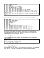
Each spdc command accepts either string or number argument where it
excepts a number. This makes it possible to write your netlist using Octave's
command format (which just accepts string arguments) like Spice netlist style.
For example, the following statements will perform the same “ac” simulation.
sp_ac dec 10 1e+3 1e+9
sp_ac('dec','10','1e+3','1e+9')
sp_ac('dec',10,1e+3,1e+9)
sp_ac dec n=10 fstart=1e+3 fstop=1e+9
sp_ac('dec','n=10','fstart=1e+3','fstop=1e+9')
n=10;fstart=1e+3;fstop=1e+9; sp_ac('dec',n,fstart,fstop)
Octave's native statements are helpful, for example, to process data or figures,
to perform parameter sweep simulation using loop or conditional branch, and
so on.
Octave's syntax supports the Sha-Bang “#!”. Thus you can even make your
spdc netlist a standalone executable by adding the following line to the head
of netlist and adding executable permission to the file.
#!/usr/bin/env spdc
Then you can run simulation by either of the following shell commands.
$ spdc your-circuit-netlist-file
$ ./your-circuit-netlist-file
3.
Modeling 3D Distributed Circuit
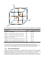
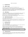
In spdc, 3D distributed circuit in a cuboid zone is discretized to repeated
cubic circuit cells. The following figure shows one of the cubic cells, where “n”
means circuit node, “b” means circuit branch, “e” means electric circuit, “m”
means magnetic circuit.
z
ne
bey
bex
bmz
ne
bex
bey
ne
bez
bmx
bmy
bez
nm
bez
bmy
bmx
ne
ne
bez
bey
bex
x
ne
ne
bmz
bey
y
bex
ne
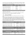
In this model, electric circuit and magnetic circuit are interlaced, the cell size
(branch length) is 2 grids, so each cell contains 8 grids which are listed below.
Grid type
Symbol
Position in the cell
Electric circuit node
ne
[0 0 0]
Electric circuit branch (along x-direction)
bex
[1 0 0]
Electric circuit branch (along y-direction)
bey
[0 1 0]
Electric circuit branch (along z-direction)
bez
[0 0 1]
Magnetic circuit node
nm
[1 1 1]
Magnetic circuit branch (along x-direction)
bmx
[0 1 1]
Magnetic circuit branch (along y-direction)
bmy
[1 0 1]
Magnetic circuit branch (along z-direction)
bmz
[1 1 0]
Thus, in spdc each node or branch can be identified by its unique 3D
coordinate, compared with Spice in which node or branch is identified by its
name. This is a main difference between spdc netlist and Spice netlist.
3.1.
Circuit Parameters
In spdc, the circuit's cuboid size (sc) should be set first of all, which specifies
the whole simulate zone. Then every object's 3D coordinate (x, y, z) should be
limited in the range of the cuboid size, i.e. 1≤x≤scx, 1≤y≤scy, 1≤z≤scz.
The boundary condition (bc) also should be given. spdc provides two types of
boundary condition, including short electro circuit (open magnet circuit) and
open electro circuit (short magnet circuit). Other types of boundary condition
can be realized by set circuit parameters near the boundary to proper values.
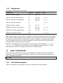
Circuit parameters include the following.
Parameter
Symbol
Position
Value
Electro branch conductance
gc
σ e (2⋅dx)
Electro branch capacitance
cc
[1 0 0]
[0 1 0]
[0 0 1]
Magnet branch conductance
rc
σ m (2⋅dx )
Magnet branch capacitance
lc
[0 1 1]
[1 0 1]
[1 1 0]
ϵ 0 ϵr (2⋅dx)
μ 0 μ r (2⋅dx )
Magnet capacitance can be set to zeros if you do not want to take account of
“inductance” in simulation.
Magnet conductance can be set to zeros if magnetic medium's loss can be
ignored (and if there is no “magnetic monopole” in the world).
3.2.
Ports and Stimuli
Stimuli include branch voltage source and branch current source as Spice
does.
Instead of directly adding stimuli to the circuit branches, the electro/magnet
circuits together are first labeled with several voltage ports and several
current ports (see below tables), each port is then defined with a direction
vector, and finally add stimuli to each port. As a result, all the zones which
belong to the same port will be added with the same stimulus along the same
direction. This makes it easy to set stimuli because the port number is usually
much smaller than the branch number.
Parameter
Symbol
Position
Value
Electro branch voltage port index
vpe
voltage port index
Electro branch current port index
ipe
[1 0 0]
[0 1 0]
[0 0 1]
Magnet branch voltage port index
vpm
voltage port index
Magnet branch current port index
ipm
[0 1 1]
[1 0 1]
[1 1 0]
Parameter
Symbol
Index
Value
Branch voltage port direction vector
vd
vpe,vpm
[vdx, vdy, vdz]
Branch current port direction vector
id
ipe,ipm
[idx, idy, idz]
current port index
current port index
Parameter
Symbol
Index
Value
Branch voltage port source
vs
vpe,vpm
E s (2⋅dx) , H s (2⋅dx)
Branch current port source
is
ipe,ipm
J es (2⋅dx )2 , J ms (2⋅dx )2
3.3.
Responses
Responses include the following.
Parameter
Symbol
Position
Value
ϕE
Electro node voltage
ve
[0 0 0]
Electro branch motiveforce
fe
Electro branch voltagedrop
de
[1 0 0]
[0 1 0]
[0 0 1]
Electro branch current
ie
Magnet node voltage
vm
[1 1 1]
ϕH
Magnet branch motiveforce
fm
H A (2⋅dx )
Magnet branch voltagedrop
dm
[0 1 1]
[1 0 1]
[1 1 0]
Magnet branch current
im
E A (2⋅dx)
E ϕ (2⋅dx)
J e (2⋅dx)2
H ϕ (2⋅dx)
J m (2⋅dx )2
The node voltage is the scalar potential of branch voltagedrop which satisfies
KVL, while branch motiveforce can also be considered as the vector potential
of branch current which satisfies KCL. spdc's simulate command only gives
those potentials which are less redundant. All the other data will be got by
post-simulation data process method.
Besides, voltagedrop plus motiveforce just equals the total field ( E ϕ + E A=E ,
H ϕ + H A= H ) which is concerned by electromagnet field simulators, while
spdc mainly concerns voltage and current as Spice does.
4.
spdc Commands
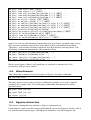
Once you start spdc and get into the interpreter, begin with the following
command to list all spdc commands, and then see the separate help text for
each command for detail.
sp_help
4.1.
Circuit Description
These commands correspond to Spice's instantiation statements.
sp_circ
sp_circ
sp_circ
sp_circ
sp_circ
sc SCX [SCY SCZ]
bc 0|1
gc|rc|cc|lc X Y Z VALUE
vpe|vpm|ipe|ipm X Y Z PORT
vd|id PORT DIRX DIRY DIRZ
sp_stim vs|is PORT
sp_stim vs|is PORT
sp_stim vs|is PORT
[PW [PER]]]]]]
sp_stim vs|is PORT
[PHASE]]]]]
[ac [MAG [PHASE]]] [dc [VALUE]]
[ac [MAG [PHASE]]] [pwl T1 V1 [T2 V2 ...]]
[ac [MAG [PHASE]]] [pulse V1 V2 [TD [TR [TF
[ac [MAG [PHASE]]] [sin VO VA [FREQ [TD [THETA
spdc also provides the following commands to help you draw complex
geometric patterns conveniently.
sp_draw
sp_draw
sp_draw
sp_draw
sp_draw
sp_draw
sp_draw
sp_draw
sp_draw
sp_draw
sp_draw
ls|rm ...
mv|cp PARAM VALUE ...
im X Y Z FILE ...
ex Z FILE ...
all ...
new X Y Z ...
[mov|ext][drw] shf N DIST TX TY TZ ...
[mov|ext][drw] rot N PHASE PX PY PZ TX TY TZ ...
[mov|ext][drw] pnt N SCALE PX PY PZ ...
[mov|ext][drw] axs N SCALE PX PY PZ TX TY TZ ...
[mov|ext][drw] pln N SCALE PX PY PZ NX NY NZ ...
Notice each type of data's cell position; to set value to a datum out of its
position(s) will take no effect. One method to avoid this is to extend your
pencil size to at least the cell size, 2×2×2.
4.2.
Analyses
These commands are as the same as the corresponding Spice commands
(.op, .ac, .tran).
sp_op
sp_ac lin|oct|dec N FSTART FSTOP
sp_tran TSTEP TSTOP [TSTART]
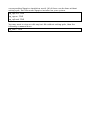
4.3.
Output Control
Not only spdc can plot curves of waveform/spectrum as Spice's .plot command
does, but also it can plot 3D distributions of data like field simulators.
sp_plot
sp_plot
sp_plot
sp_plot
sp_plot
sp_plot
sp_plot
sp_plot
sp_plot
sp_plot
sp_plot
tran vs|is PORT [UNIT] ...
tran ve|vm X Y Z [UNIT] ...
tran fex|fey|fez|fmx|fmy|fmz X Y Z [UNIT]
tran dex|dey|dez|dmx|dmy|dmz X Y Z [UNIT]
tran iex|iey|iez|imx|imy|imz X Y Z [UNIT]
ac vs|is(r|i|m|p) PORT [UNIT] ...
ac ve|vm(r|i|m|p) X Y Z [UNIT] ...
ac fex|fey|fez|fmx|fmy|fmz(r|i|m|p) X Y Z
ac dex|dey|dez|dmx|dmy|dmz(r|i|m|p) X Y Z
ac iex|iey|iez|imx|imy|imz(r|i|m|p) X Y Z
[linlin|linlog|loglin|loglog] ...
sp_plot3
sp_plot3
sp_plot3
sp_plot3
...
...
...
[UNIT] ...
[UNIT] ...
[UNIT] ...
dc|tran|ac gc|rc|cc|lc|vpe|vpm|ipe|ipm[n] [UNIT] ...
dc fe|fm|de|dm|ie|im[n] [UNIT] ...
tran fe|fm|de|dm|ie|im[n] T [UNIT] ...
ac fe|fm|de|dm|ie|im[n](r|i) F [UNIT] ...
spdc's set circuit and simulate commands only give basic (packed) data, since
this can save memory and all the other data can be calculated from them.
Therefore, you should calculate (unpack) the data before plotting them. The
following commands manipulate the unpacked data.
sp_post [gc|rc|cc|lc|vpe|vpm|ipe|ipm ...]
sp_post [ve|vm|fe|fm|de|dm|ie|im ...]
sp_reset [gc|rc|cc|lc|vpe|vpm|ipe|ipm ...]
sp_reset [ve|vm|fe|fm|de|dm|ie|im ...]
Notice each type of data's cell position; to evaluate a datum out of its
position(s) will get zero values.
4.4.
Miscellaneous
The following command is as the same as Spice's .include command.
sp_include FILE
You may want to save your circuit or simulation results so as not to spend
cputime on it again later. The following commands manipulate the basic
(packed) data.
sp_save FILE [c|r|a]
sp_load FILE [c|r|a]
sp_clear [c|r|a]
4.5.
Ngspice Interactive
The above commands are similar to Spice's command set.
Furthermore, spdc can also export distributed circuit to Ngspice netlist, edit it
for stimuli and analysis type, call Ngspice simulator, and then import the
corresponding Ngspice simulation result. All of these can be done without
exiting spdc, but this needs Ngspice installed on your system.
sp_nglist FILE
sp_ngrun FILE
sp_ngload FILE
You may want to view or edit any text file without exiting spdc, then the
following command does.
sp_edit FILE