Download "user manual"

1
MEM800-007
Chapter 4a
Linear Matrix Inequality Approach
Reference: Linear matrix inequalities in system and control theory, Stephen
Boyd et al. SIAM 1994.
Linear Matrix Inequality (LMI) approach have become a powerful design tool
in almost all areas of control system engineering. The LMI approach has the
following advantages:
• Many control system design specifications and constraints can be
expressed as LMIs.
• The LMI problems can be solved numerically very efficiently using
interior-point methods.
• For those problems that analytical solutions are impossible, the LMI
approach often can provide solutions numerically.
LMI
A linear matrix inequality (LMI) has the form
m
F ( x) = F0 +  xi Fi > 0
(4.1)
i =1
where x ∈ R m is the variable the symmetric matrices Fi ∈ R n×n , i = 0,1,..., m,
are given.
Positive definite matrix
F ( x) > 0 means that F ( x) is positive definite, i.e., u T F ( x)u > 0 for all
nonzero u ∈ R n .
Affine function:
f ( x1 , x2 ,..., xm ) = x1a1 + x2 a2 + .... + xm am + b
2
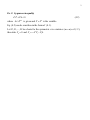
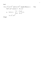
Ex .0 Lyapunov inequality
AT P + PA < 0
(4.2)
where A ∈ R n×n is given and P = PT is the variable.
Eq. (4.2) can be rewritten in the form of (4.1).
Let P1 , P2 ,...., Pm be a basis for the symmetric n × n matrices ( m = n(n + 1) / 2 ),
then take F0 = 0 and Fi = − AT Pi − Pi A .
3
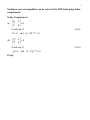
Nonlinear convex inequalities can be converted to LMI form using Schur
complements.
Schur Complenment
Q
(a)  T
S
S
>0
R 
if and only if
and Q − SR −1S T > 0 .
R>0
Q
(b)  T
S
S
>0
R 
if and only if
Q>0
Proof:
(4.3a)
and R − S T Q −1S > 0 .
(4.3b)
4
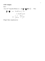
LMI Examples
Ex.1
Z ( x) ∈ R p×q depends affinely on x, and Z ( x) = σ [ Z ( x) ] .
Z ( x) < 1
⇔
Z ( x) Z T ( x) < I , i.e.,
I − Z ( x) Z T ( x) > 0
⇔
Z ( x) 
 I
 Z T ( x)
>0
I


Proof: Schur complement (a).
Then
5
Ex.2
c( x) ∈ R n , P( x) = PT ( x) ∈ R n×n depends affinely on x.
cT ( x) P −1 ( x)c( x) < 1 , P( x) > 0
⇔
 P( x) c( x) 
>0
 cT ( x )

1 

Proof: Schur complement (b).
Then
6
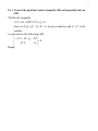
Ex.3
P( x) = PT ( x) ∈ R n×n and S ( x) ∈ R n× p depend affinely on x.
Tr ( S T ( x) P −1 ( x) S ( x) ) < 1 , P( x) > 0
⇐
Tr ( X ) < 1 ,
 X
S T ( x) 

>0 ,
S
(
x
)
P
(
x
)


X = X T ∈ R p× p
Proof:
Then
7
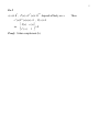
Ex.4 Convert the quadratic matrix inequality (Riccati inequality) into an
LMI
The Riccati inequality,
AT P + PA + PBR −1 BT P + Q < 0
where A, B, Q = QT , R = RT > 0 are given matrices and P = PT is the
variable,
is equivalent to the following LMI:
 − AT P − PA − Q PB 

 > 0.
T
B
P
R


Proof:
8
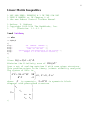
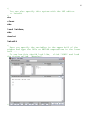
Linear Matrix Inequalities
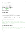
% LMI-LAB DEMO: EXAMPLE 8.1 IN THE Old LMI
% USER'S MANUAL or IN Chapter 9 of
% the new Robust Control Toolbox Manual
% Author: P. Gahinet
% Copyright 1995-2004 The MathWorks, Inc.
%
$Revision: 1.1.6.1 $
load lmidem;
>> who
>> A,B,C
%{
disp('
disp('
disp('
disp('
disp('
%}
LMI CONTROL TOOLBOX ');
********************* ');
DEMO OF LMI-LAB
');
Specification and manipulation of LMI systems ');
Example 8.1 of the Tutorial Section');
%{
−1
Given G ( s ) = C ( sI − A) B .
−1
Minimize the H-infinity norm of DG ( s ) D
Over a set of scaling matrices D with some given structure.
This problem arises in Mu theory (robust stability analysis)
The system of LMIs is:
 AT X + XA + C T SC XB 

 < 0, X > 0, S > I
T
B
X
−
S


T
where X
is symmetric, S = D D is symmetric block
diagonal with prescribed structure
 s11

S=



%}
s11
s22
s23



s23 

s33 
9
%{
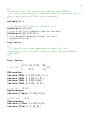
To specify this LMI system with LMIVAR and LMITERM,
(1) resets the internal varibales used for creating LMIs so
that a new system of LMIs can be created.
%}
setlmis([]);
% (2) define the 2 matrix variables X,S
X=lmivar(1,[6 1]);
% X is a 6x6 full symmetric matrix variable
S=lmivar(1,[2 0;2 1]);
% S is diag{2x2 diagonal block, 2x2 full
% symmetric block}
help lmivar
%{
(3) specify the terms appearing in each LMI. For
convenience, you can give a name to each LMI with NEWLMI
(optional)
%}
help limterm
 AT X + XA + C T SC XB 
% 1st LMI 
<0
T
−S 
B X

BRL=newlmi;
lmiterm([BRL 1 1 X],1,A,'s');
lmiterm([BRL 1 1 S],C',C);
lmiterm([BRL 1 2 X],1,B);
lmiterm([BRL 2 2 S],-1,1);
X >0
Xpos=newlmi;
lmiterm([-Xpos 1 1 X],1,1);
% 2nd LMI
% 3rd LMI
S>I
Slmi=newlmi;
lmiterm([-Slmi 1 1 S],1,1);
lmiterm([Slmi 1 1 0],1);
10
%{
(4) get the internal description of this LMI system with
GETLMIS
%}
lmisys=getlmis;
%{
Done! A full description of this LMI system is now stored
in the MATLAB variable LMISYS
%}
%{
You can retrieve various information about the LMI system
you just defined
%}
% number of LMIs:
lminbr(lmisys)
% number of matrix variables:
matnbr(lmisys)
% variables and terms in each LMI (type q to % exit lmiinfo):
lmiinfo(lmisys)
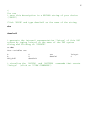
LMI
ORACLE
-------------This is a system of 3 LMI(s) with 2 matrix variables
Do you want information on
(v) matrix variables
(l) LMIs
(q) quit
?> v
Which variable matrix (enter its index k between 1 and 2) ? 1
X1 is a 6x6 symmetric block diagonal matrix
its (1,1)-block is a full block of size 6
-------------This is a system of 3 LMI with 2 variable matrices
Do you want information on
(v) matrix variables
?> ……….
(l) LMIs
(q) quit
11
?> q
It has been a pleasure serving you!
%{
We now call FEASP to solve our system of LMIs
( A'X + XA + C'SC
(
(
B'X
XB )
)
-S )
<
0
X
>
0
S
>
I
%}
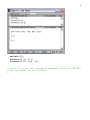
[tmin,xfeas]=feasp(lmisys);
%{
tmin=-1.839011 < 0 : the problem is feasible!
-> there exists a scaling D such that
DG ( s ) D −1
∞
<1
The output XFEAS is a feasible value of the vector of
decision variables (the free entries of X and S).
%}
xfeas
%{
Use DEC2MAT to get the corresponding values of the matrix
variables X and S:
%}
Xf=dec2mat(lmisys,xfeas,X)
Sf=dec2mat(lmisys,xfeas,S)
eig(Xf)
eig(Sf)
% the constraints
% satisfied!
X > 0
and
S > I are
12
%{
To verify that the first LMI is satisfied,
(1) evaluate the LMI system for the computed decision
vector XFEAS:
%}
evlmi = evallmi(lmisys,xfeas);
%{
(2) get the values of the left and right-hand sides of the
first LMI with SHOWLMI:
%}
[lhs1,rhs1]=showlmi(evlmi,1);
eig(lhs1-rhs1)
% the first LMI is indeed satisfied.
%{
(3) get the values of the left and right-hand sides of the
second LMI with SHOWLMI:
%}
[lhs2,rhs2]=showlmi(evlmi,2)
>> eig(rhs2)
%{
(4) get the values of the left and right-hand sides of the
third LMI with SHOWLMI:
%}
[lhs3,rhs3]=showlmi(evlmi,3)
eig(rhs3(3:4,3:4))
%{
13
Finally, let us check that the H-infinity norm of G(s)
was not less than one from the start. To do this, we can
remove the scaling D by setting S = 2*I and solve the
resulting feasibility problem:
Find X such that
( A'X + XA + C'C
(
(
B'X
XB )
)
-I )
<
X
0
>
0
This new LMI system is derived from the previous one by
setting S = 2*I with SETMVAR:
%}
newsys=setmvar(lmisys,S,2);
>> lmiinfo(newsys)
LMI
ORACLE
-------------This is a system of 3 LMI(s) with 1 matrix variables
Do you want information on
(v) matrix variables
?> q
(l) LMIs
(q) quit
It has been a pleasure serving you!
%
%
Now call FEASP to solve the modified LMI
problem:
[tmin,xfeas]=feasp(newsys);
These LMI constraints were found infeasible
%
%
Infeasible! The H-infinity norm of
was larger than one
G(s)
14
%{
You can also specify this system with the LMI editor:
>> lmiedit
%}
who
clear
who
load lmidem;
who
demolmi
lmiedit
%{
Here you specify the variables in the upper half of the
window and type the LMIs as MATLAB expressions in the lower
half ...
To see how this should look like, click "LOAD" and load
the string called "demolmi".
%}
15
%{
You can
* save this description in a MATLAB string of your choice
("SAVE")
Click “SAVE” and type demolmi2 as the name of the string
who
demolmi2
* generate the internal representation "lmisys" of this LMI
system by typing lmisys2 as the name of the LMI system
string and clicking on "CREATE"
>> who
Your variables are:
A
B
ZZZ_ehdl
S
X
demolmi2
ans
demolmi
* visualize the LMIVAR and LMITERM
"lmisys" (click on "VIEW COMMANDS")
lmisys2
C
commands that create
16
setlmis([]);
X=lmivar(1,[6
S=lmivar(1,[2
1]);
0;2 1]);
* write in a file this series of commands (click on "WRITE")
Click on "CLOSE" to exit LMIEDIT
%}
17
Example 8.2
% EXAMPLE 8.2 IN THE Old LMI USER'S MANUAL
% or IN Chapter 9 of the Robust Control
% Toolbox Manual
A=[-1 -2 1;3 2 1;1 -2 -1];
B=[1;0;1];
Q=[1 -1 0;-1 -3 -12;0 -12 -36];
%{
Consider the optimization problem
Minimize Trace(X) subject to
A'X + XA + XBB'X + Q < 0
(9-9)
It can be shown that the minimizer X* is simply the
stabilizing solution of the algebraic Riccati equation
A'X + XA + XBB'X + Q = 0
This solution can be computed directly with the Riccati
solver care and compared to the minimizer returned by mincx.
From an LMI optimization standpoint, problem (9-9) is
equivalent to the following linear objective minimization
problem:
Minimize Tr(X) subject to
[ A'X+XA+Q
XB ] < 0
[
B'X
-I ]
Since Trace(X) is a linear function of the entries of X,
this problem falls within the scope of the mincx solver and
can be numerically solved as follows:
%}
%{
(1) Define the LMI constraint (9-9) by the
sequence of commands
%}
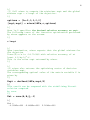
setlmis([]);
18
X = lmivar(1,[3 1])
% variable X, full symmetric
lmiterm([1 1 1
lmiterm([1 1 1
lmiterm([1 2 2
lmiterm([1 2 1
[ A'X+XA+Q
%
%
[
X],1,A,'s');
0],Q);
0],-1);
X],B',1);
B'X
XB ]
-I ]
LMIs = getlmis;
lmiinfo(LMIs)
LMI
ORACLE
-------------This is a system of 1 LMI(s) with 1 matrix variables
Do you want information on
(v) matrix variables
?> q
(l) LMIs
(q) quit
It has been a pleasure serving you!
%{
(2) Write the objective Trace(X) as c'x where x is the
vector of free entries of X. Since c should select the
diagonal entries of X, it is obtained as the decision vector
corresponding to X = I, that is,
%}
c = mat2dec(LMIs,eye(3))
%{
Note that the function defcx provides a more systematic way
of specifying such objectives (see “Specifying c'x
Objectives for mincx” on page 9-37 for details).
%}
help defcx
19
%{
(3) Call mincx to compute the minimizer xopt and the global
minimum copt = c'*xopt of the objective:
%}
options = [1e-5,0,0,0,0]
[copt,xopt] = mincx(LMIs,c,options)
%{
Here 1e-5 specifies the desired relative accuracy on copt.
The following trace of the iterative optimization performed
by mincx appears on the screen:
%}
c'*xopt
%{
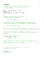
Upon termination, mincx reports that the global minimum for
the objective
Trace(X)=c'x is –18.716695 with relative accuracy of at
least 9.5-by-10^–6.
This is the value copt returned by mincx.
%}
%{
(4) mincx also returns the optimizing vector of decision
variables xopt.
The corresponding optimal value of the matrix variable X is
given by
%}
Xopt = dec2mat(LMIs,xopt,X)
%{
This result can be compared with the stabilizing Riccati
solution computed
by care:
%}
Xst = care(A,B,Q,-1)
%{
Xst =
-6.3542e+000 -5.8895e+000
2.2046e+000
20
-5.8895e+000 -6.2855e+000 2.2201e+000
2.2046e+000 2.2201e+000 -6.0771e+000
%}
norm(Xopt-Xst)
help norm