Download Rocking Curves - Characterization Facility

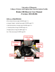
University of Minnesota
College of Science and Engineering Characterization Facility
PANalytical X’pert Pro High Resolution Specular and
Rocking Curve Scans User Manual
(Version: 2012.10.17)
The following instructions are meant to be a guide, but many of the scan parameters may change
based on your samples and experience. Please note that the optics are delicate; do not bump or
drop the optic housing units. If the x-rays are off, NEVER attempt to turn them back on unless
specifically instructed by an x-ray scattering lab staff member.
Hardware setup
1. The system must be setup with the x-ray tube using the line source. The hybrid
monochromator must be mounted on the incident beam side. Make sure the beam attenuator
cable is plugged into the hybrid. Install the ½ divergence slit into the hybrid module, and if
the sample is less than 25 mm an appropriate beam mask should be inserted.
1
2. The rocking curve (RC) + triple axis mount must be attached on the diffracted beam side with
Detector 1 attached to the triple axis position (if you are going to use triple axis mode) and
Detector 2 attached to the rocking curve position (if you are going to use rocking curve
mode). While a variety of diffracted beam slits can be installed to improve resolution, a ½
slit should be installed for general purpose scanning.
Note: The following are the definitions of the angles in the software:
ω – angle between incident x-rays and sample surface
2θ – angle between incident x-rays and detector
ψ – azimuthal sample tilt
φ – in-plane sample rotation
x,y – horizontal and vertical position of sample, respectively
z – sample height
φ
ω
2θ
ψ
2
User setup
3. Log onto the computer: User: Charfac code # (for example 2310); Password; Domain:
CharFac.
4. Open the Data Collector program.
5. Enter your user name (created during training) and password.
6. Select Instrument/Connect in the Data Collector. The Go On Line box will appear.
7. Select High Resolution as the Configuration and RC as the Beam Path. Then press the OK
button.
8. A message dialog box will appear. Any line with a yellow triangle tells what the software is
assuming. Press the OK button. If a red stop sign appears, you cannot continue, please find
an x-ray staff member for assistance.
9. If you previously had set sample offsets, a dialog may appear asking if you want to apply
these offsets. Yes keeps the sample offsets, No clears them. Unless you were the last person
to use the machine, it is a very good idea to clear the offsets.
Optics setup
10. Select the Incident Beam Optics tab and double click on one of the item lines:
a. PreFIX Module: Ge 4-bounce hybrid.
b. Divergence Slit: 1/2o divergence slit
c. Beam Attenuator: Ni 0.125 mm automatic, Usage should be Do Not Switch and
the Activated box should be checked. It is highly recommended to cycle from
Activated → Deactivated → Activated to check if the attenuator is working
properly.
d. Mask: Select appropriate size Inc. Mask Fixed 5,10,15,20 mm (MPD/MRD).
11. Select the Diffracted Beam Optics tab and double click on one of the item lines:
a. PreFix Module: Triple Axis (Rocking Curve Optics).
b. Receiving Slit: Parallel Plate Collimator Slit.
c. Detector: Mini prop large window 2 and the Wavelength is K alpha 1.
12. Optional: If you will be using the triple axis detector, right mouse click on Triple Axis in the
Diffracted Beam Optics window tab and select Activate. The PreFix Module should be
selected to be the Triple Axis (Monochromator 3 Bounce). Make sure the Detector is mini
prop large window 1 and the Wavelength is K alpha 1.
13. Select the Instrument Settings tab, double click an item, select the X-ray tab, and set the
Generator to 45 kV and 40 mA.
3
Sample mounting
14. Select the Instrument Settings tab, double click an item, select the Position tab, set all
positions to either 0o or 0 mm. Press the Apply button to move the stage.
15. Remove the sample holder by rotating until it releases.
16. Mount the sample as flat as possible on the stage with double sided tape or spring clips for
large wafer samples. If the sample is larger than 5 mm, mount the long axis of the sample
along the beam direction (i.e. horizontal, x-direction). If the sample is less than 5 mm, mount
the long axis azimuthally to the beam direction (i.e. vertical, y-direction). These alignments
will assist in providing the lowest background noise and maximizing signal strength.
17. Load the sample holder into the system.
Checking the zero position and direct beam intensity
18. Go to the Measure menu and select Manual Scan.
19. The Manual Scan window will appear. Enter into the following fields: Scan Axis: 2theta,
Scan Mode: Continuous, Range: 2.0o, Step Size: 0.005 , and Time per Step: 0.1 s. Press the
Start button to begin the scan.
20. After the scan is finished, right mouse click on the graph and select Peak Mode.
21. To accept the location of the peak, press the Move To button and then select OK. To select a
different position of the peak, press Cancel, right mouse click on the graph, and select Move
Mode. This will move the goniometer to the user defined position.
22. Once the correct position of the detector is found, click on the Tools menu and select Sample
Offsets. Set 2theta = 0.0o and select OK button. This will correct for the zero position and
make the current 2θ value 0.0o.
4
Setting the correct sample height and horizontal tilt
23. The correct sample height has been aligned when the sample bisects the direct incident beam
it reduces the direct beam intensity to ½ the original value.
24. Select the Instrument Settings tab, double click an item, select the Position tab, set Z to 7.0
mm. Press the OK button to move the stage
25. Go to the Measure menu and select Manual Scan.
26. The Manual Scan window will appear. Enter into the following fields: Scan Axis: Z, Scan
Mode: Continuous, Range: 4.0 mm, Step Size: 0.01 mm, and Time per Step: 0.1 s. Press the
Start button to begin the scan.
27. The graph should look like a Heaviside step function with high intensity at low Z values and
zero intensity at high Z values. Using Move Mode, move the green cursor until the intensity
is ½ of the maximum intensity in the low Z range.
a. If the Heaviside step has an “intermediate step” in it, move the green cursor to the
Z value that halves the intensity between the maximum intensity in the low Z
range and the intermediate step. This intermediate step usually occurs when the
sample’s vertical width (y-direction) is smaller than the beam mask.
28. Return to the Manual Scan window. Enter into the following fields: Scan Axis: Omega, Scan
Mode: Continuous, Range: 4.0o, Step Size: 0.01 , and Time per Step: 0.1 s. Press the Start
button to begin the scan.
29. Use either Move Mode or Peak Mode (preferred) to center to the observed peak.
30. Repeat steps 26 – 27 until both Z and omega positions do not change significantly. A good
simple guide is that Z should not shift more than 0.01 mm in subsequent iterations
31. Once the optimum values have been found, click on the Tools menu and select Sample
Offsets. Set the Omega value to 0.0o. This will make the current ω value read as 0.0o
Peak Optimization
32. It is highly recommended to align the sample in subsequent steps with respect to a known
crystallographic plane. The best choice for this is to use a known substrate peak. The
Collector software has a large database of common substrates pre-loaded, but it is also
possible to load new substrates into the database.
a. Select Customize/Unit cells and then press the insert button.
b. Enter all the requested information for the unit cell. The primary and secondary
hkl are the growth vector and a wafer flat vector respectively. (If no wafer flat is
present any vector perpendicular to the growth vector is sufficient.) The hkl
values must be entered as integers with spaces between them.
5
c. After entering the all the information, press the OK button and notice the new cell
added to the list. Then press the OK button.
33. Select Customize/Options and make sure the radio button in front of Single Crystal mode is
checked. Close this window.
34. If the scan will be performed in Triple Axis mode, it is still much easier to initially find the
peak in rocking curve mode and then switch to triple axis for the final alignment. To switch
between the modes, right mouse click on Triple Axis or Rocking Curve in the Diffracted
Beam Optics window tab and select Activate.
35. Before a scan is collected for an extended measuring time, preliminary scans are usually done
to optimize the peak(s) of interest. This is done using manual alignment measurements of ω
and ψ.
36. In Instrument Settings tab, double click on an item, select the Position tab, and select the
substrate material in the unit cell field.
a. If unit cell information was not entered, enter the 2θ value for the peak of interest
in the 2theta field and 0 in the Offset field and press the OK button. Continue to
Step 40.
37. Enter the plane of interest in the HKL field. This will set all the angles to the theoretical
values for this crystallographic plane. Then press the OK button.
38. Select Measure/Manual Scan from the main menu.
39. Return to the Manual Scan window. Enter into the following fields: Scan Axis:
2theta/Omega, Scan Mode: Continuous, Range: 2.0o, Step Size: 0.01 , and Time per Step: 0.2
s. Press the Start button to begin the scan.
40. After the scan is finished, use Move Mode or Peak Mode (preferred) to center onto the most
intense peak.
a. Ideally if the initial zero alignments were done correctly, the center of the peak
should line up with the theoretical value of the (hkl) plane that was aligned. In
reality this is can be difficult due to not aligning the z-axis perfectly, causing a
“sample displacement error” in peak positions. This shift is often very minor, and
can be corrected using numerous models. The JADE software has an excellent
displacement error correction routine and is highly recommended.
41. Return to the Manual Scan window. Enter into the following fields: Scan Axis: Omega, Scan
Mode: Continuous, Range: 1.0o, Step Size: 0.005 , and Time per Step: 0.3 s. Press the Start
button to begin the scan.
42. After the scan is finished, right mouse click on the graph, select Axes, and choose linear for
the Type of scale for the graph. Using Move Mode or Peak Mode (preferred), center onto the
most intense peak.
6
43. Return to the Manual Scan window. Enter into the following fields: Scan Axis: Psi, Scan
Mode: Continuous, Range: 6.0o, Step Size: 0.01 , and Time per Step: 0.3 s. Press the Start
button to begin the scan.
44. After the scan is complete, select either Move Mode or Peak Mode (preferred) to center
onto the measured peak.
45. Optional: If the sample is smaller than 5 mm in the vertical direction (y-direction), a ydirection scan might be needed to make sure that the sample is aligned vertically.
a. To do this return to the Manual Scan window. Enter into the following fields:
Scan Axis: y, Scan Mode: Continuous, Range: 10.0 mm, Step Size: 0.1 mm, and
Time per Step: 0.5 s. Press the Start button
b. After the scan is complete, select either Move Mode or Peak Mode (preferred) to
center onto the measured peak.
c. Repeat Steps 41-42.
46. Return to the Manual Scan window. Enter into the following fields: Scan Axis: Omega, Scan
Mode: Continuous, Range: 0.5o, Step Size: 0.005 , and Time per Step: 0.5 s. Press the Start
button to begin the scan
47. After the scan is complete, select either Move Mode or Peak Mode (preferred) center onto
the measured peak.
48. Repeat Steps 39 – 45 until the positions of ω, ψ, and y (optional) do not move significantly.
Usually one or two iterations are needed.
49. Once the optimum values have been found, click on the Tools menu and select Sample
Offsets. Set the Omega value to exactly ½ of the current 2theta value.
50. Back in the control window select the Incident Beam Optics tab. Double click on an item
related to the beam attenuator. Change the Usage field to Switch at preset intensity, set the
Activate Level to 500,000, and the Deactivate Level to 400,000.
7
Measurement Program
51. Select File/New Program/Relative scan for a rocking curve and Relative scan or Absolute
Scan for a coupled scan. A relative scan is centered on the current position of the goniometer.
An absolute scan scans a specific range of angles and is often used for coupled scans.
52. Make sure that the desired Rocking Curve or Triple Axis setting is selected as the Secondary
Beam Path. The Scan Axis should be omega for a rocking curve and 2theta-omega for a
coupled scan (omega-2theta is also a coupled scan but the reference angle is ω instead of 2θ).
The Scan Mode is typically set to continuous and the Time Per Step should be in the range of
0.5 – 5.0 s. It is important to remember that these are suggested values and the actual
parameters needed for each measurement will vary upon the sample.
53. Select File/Save as and enter a name for the program and then press the OK button. Close
this window.
54. Select Measure/Program/Relative scan or Absolute Scan depending on which type of
program was created above.
When Done
55. Make sure the attenuator is set to Switch at Preset Intensity or Do Not Switch Activated.
56. Power the x-rays down to 40 kv and 10 ma.
57. Close the program, transfer your data (files are not backed up), and log off the computer.
Files can be viewed with the Data Viewer program and converted to ascii text files if
desired. Please leave the work area clean.
Remember CharFac is a user facility, and we all need to do our part to
keep the work area clean!
8