1
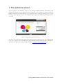
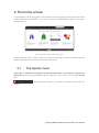
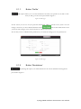
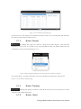
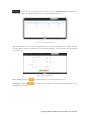
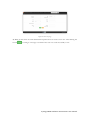
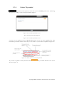
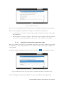
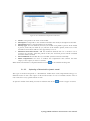
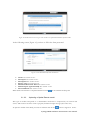
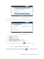
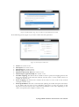
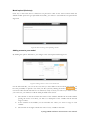
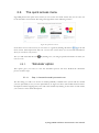
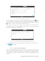
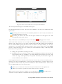
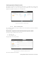
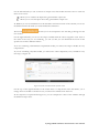
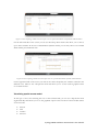
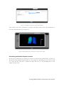
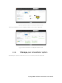
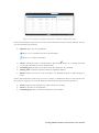
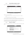
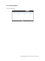
User manual for the Simulation Environment Synergy-COPD simulation environment. User manual Index Introduction .......................................................................................................................................................................... 5 1. The welcome screen .................................................................................................................................................. 6 2. The home screen ........................................................................................................................................................ 7 2.1. 2.1.1. Button ‘Profile’ ....................................................................................................................................... 8 2.1.2. Button ‘Simulations’ .............................................................................................................................. 8 2.1.3. Button ‘Recent’ ...................................................................................................................................... 9 2.1.4. Button ‘Pending’ .................................................................................................................................... 9 2.1.5. Button ‘Users’ ......................................................................................................................................... 9 2.1.6. Button ‘My models’ ............................................................................................................................. 11 2.1.7. ‘Search for models’ option ................................................................................................................. 20 2.1.8. ‘Log-off’ option .................................................................................................................................... 20 2.2. 3. The top-bar menu ............................................................................................................................................ 7 The quick access menu ................................................................................................................................. 21 2.2.1. ‘Simulate’ option .................................................................................................................................. 21 2.2.2. ‘Manage your simulations’ option ..................................................................................................... 28 2.2.3. ‘Comorbidity analysis’ option ............................................................................................................ 30 2.2.4. ‘About us’ option ................................................................................................................................. 30 Annex ......................................................................................................................................................................... 33 Synergy-COPD simulation environment. User manual List of figures Figure 1. Simulation Environment welcome screen ........................................................................ 6 Figure 2. Simulation Environment home screen ............................................................................. 7 Figure 3. Simulation Environment bar menu ................................... ¡Error! Marcador no definido. Figure 4. Profile page...................................................................................................................... 8 Figure 5. User simulations management page ................................................................................. 8 Figure 6. Recent simulations dropdown menu shows the latest simulations computed.................... 9 Figure 7. User management screen ................................................................................................. 9 Figure 8. Edit user profile page ..................................................................................................... 10 Figure 9. New user page ............................................................................................................... 10 Figure 10. List of models uploaded by the user ............................................................................. 11 Figure 11. Available options for each model uploaded ..................... ¡Error! Marcador no definido. Figure 12. Model selection type .................................................................................................... 12 Figure 13. Model selection screen. Type of the model to be uploaded is ‘deterministic compartment model’ .......................................................................................................................................... 12 Figure 14. New deterministic compartment model form ............................................................... 13 Figure 15. Model selection screen. Type of the model to be updated ‘deterministic dynamic model’ ..................................................................................................................................................... 14 Figure 16. New deterministic dynamic model form....................................................................... 14 Figure 17. Model selection screen. Type of model to be uploadad ‘spatial remote model’ ............. 15 Figure 18. New spatial remote model form ................................................................................... 15 Figure 19. Model selection page. Type of model to be uploaded ‘Bayesian model’ ........................ 16 Figure 20. New Bayesian model form ........................................................................................... 16 Figure 21. Success message after uploading a model ..................................................................... 17 Figure 22. Setting values to a new case for model ‘test’ ................................................................. 17 Figure 23. Adding output connections to model ‘Oxygen Tranposrt 2’ ......................................... 18 Figure 24. Output connection with ‘M7 ROS’ has been set ........................................................... 18 Figure 25. Quick access menu....................................................................................................... 21 Figure 26. List of models ready to be simulated ............................................................................ 22 Figure 27. The list of models is updated with the models compatible with the last one selected .... 22 Figure 28. User has to choose which cases to use as input of the simulation ................................. 23 Figure 29. Input parameters for a Bayesian model ........................................................................ 24 Figure 30. Results from a deterministic compartment model ........................................................ 24 Figure 31. Results from deterministic dynamic model ................................................................... 25 Figure 32. View comparing variables from all output cases for specific deterministic compartment model simulated ........................................................................................................................... 26 Figure 33. View comparing variables from all output cases for a specific deterministic dynamic model simulated ........................................................................................................................... 26 Figure 34. Visualization options for a spatial remote model .......................................................... 27 Figure 35. 3D visualization of the results from a spatial remote model ......................................... 27 Figure 36. Graphical visualization of the Bayesian simulation results ............................................ 28 Figure 37. Tabular visualization of the Bayesian simulation results ................................................ 28 Figure 38. List of simulations completed (left) and list of simulation waiting to finish (right) ........ 29 Figure 39. Information related to the Synergy-COPD project ....................................................... 30 Synergy-COPD simulation environment. User manual Synergy-COPD simulation environment. User manual Introduction Currently, many different tools exist aimed at simulating models that represent the human physiology. Both models and simulation environments are developed in specific languages, and are interoperable with other models represented in the same or in similar languages. Synergy-COPD simulation environment is developed to offer a common frame of simulation for models developed in different programming languages. This simulation environment is targeted to bio-researchers and medicine students, and constitutes a framework to support the observation and analyses of physiological mechanisms. Eight deterministic physiological models and one probabilistic model are considered, which are related to the respiratory chain and are represented in different languages. The purpose of this deliverable is to present the new modules added to the Simulation Workflow Management System (SWoMS): the user data base and the parallelization of model execution and the new features in the Graphical Visualization Environment (GVE). Synergy-COPD simulation environment. User manual 1. The welcome screen Figure 1 presents the Welcome screen to the Synergy-COPD simulation environment. The information presented on the right hand side correspond to the numbrer of public models, the number of simulations and the number of users registered in the system. By passing the mouse over the wings of the butterfly you can see the different options that this simulation environment allows you to do. Figure 1. Simulation Environment welcome screen You have to be registered in the system if you want to log in. If that is the case, you should be able to log in by writing your user Id and password in the boxes provided, in the top right of the screen. If your are not registered yet, please send an email to [email protected] . Synergy-COPD simulation environment. User manual 2. The home screen Congratulations! You have logged in. You should now be seeing Figure 2. This is the home screen of the simulation environment. As you can see, there are many different options. We will go through them all. Figure 2. Simulation Environment home screen First we will have a closest look to each of the options in the top bar menu to continue with the options in the quick access menu, in the centre of the screen. 2.1. The top-bar menu ¡Error! No se encuentra el origen de la referencia.¡Error! No se encuentra el origen de la referencia. shows the bar menu which is always visible. Let’s have a look to every option included here. Clicking this option allows you return to the home screen from any window. Synergy-COPD simulation environment. User manual 2.1.1. Button ‘Profile’ This option allows you to see the information stored in your profile. If you click on this link you will get to the screen presented in Figure 3 Figure 3. Profile page . In this screen you can see all your personal information which is stored in the system. You can change it and once you have finished click the button and an alert will be shown to let you know if the changes were stored correctly or if there was an error. In case that you have administration permissions you could also change your own permissions. Figure 3. Profile page 2.1.2. Button ‘Simulations’ By clicking this option you will be directed to the screen ‘Simulation management’ presented in Figure 4. Synergy-COPD simulation environment. User manual Figure 4. User simulations management page In this screen you can manage your simulations and see if there is any running. We will talk about the options presented here in Section 2.2.2. 2.1.3. Button ‘Recent’ By clicking this option you will see a drop down menu, Figure 5, with the latest simulations you have run. If you click on any of the simulations listed, you will be redirected to the visualization screen, presented in Section 2.2.1. Figure 5. Recent simulations dropdown menu shows the latest simulations computed If you click ‘More’, you will be directed to the screen ‘Simulation management’, presented in Figure 4. User simulations management page . 2.1.4. Button ‘Pending’ Clicking this option, you will see a drop down menu. If you have started one or more simulations they will be listed here. 2.1.5. Button ‘Users’ Synergy-COPD simulation environment. User manual If you can see this option, it means that you have administration permissions. By clicking this option you will be directed to the screen presented in Figure 6. Figure 6. User management screen This screen allows you to see the users registered in the system. By clicking the icon you can edit the information related to a specific user, as presented in Figure 7. You can update the information or delete a user. Figure 7. Edit user profile page When clicking the button you will return to the ‘Users management’ screen. By clicking the button can register a new user. you will see a screen like the one presented in Figure 8 where you Synergy-COPD simulation environment. User manual Figure 8. New user page By filling up this form one with administration permissions can create a new user. After clicking the button you will get a message to confirm if the user was saved successfully or not. Synergy-COPD simulation environment. User manual 2.1.6. Button ‘My models’ If you can see this option, it means that you have modeler permissions. By clicking this option you will get to the screen presented in Figure 9. Figure 9. List of models uploaded by the user In the screen presented in Figure 9 Figure 9. List of models uploaded by the user you can see the models you have uploaded previously, in case you have uploaded any. The information presented and the actions that you can make on your model are explained in Figure 10. Figure 10. Available options for each model uploaded If you want to upload a model, click the button shown in Figure 11. and you will be directed to the screen . Synergy-COPD simulation environment. User manual Figure 11. Model selection type Here you can see the different kinds of models that you can upload in the simulation environment. The two main requirements to upload your model in our simulation environment are: The model has to be able to read the input variables and their values from a file written SE-TAB format. The model has to be able to produce a file with the output variables and their generated values after execution in SE-TAB format (See Annex 4.2 for complete documentation). 2.1.6.1. Uploading a Deterministic compartment model This type of model corresponds to a deterministic model where the output variables are presented in compartments. Every compartment has a list of output variables. Every output variable has a value assigned. To upload a model of this kind, just select it and then click in the button as Figure 12 shows. Figure 12. Model selection screen. Type of the model to be uploaded is ‘deterministic compartment model’ In the following screen, presented in Figure 13, you have to fill in the form presented. Synergy-COPD simulation environment. User manual Figure 13. New deterministic compartment model form Name: corresponds to the name of the model. Descriptor: Corresponds to the variables included in the model, its descriptions and units. Description: Write a short description of the model. Privacy type: You can decide if you want your model to be public or private. If the model is private, it will only be visible by you, whereas if the model is public, all the users of the simulation environment will have the opportunity to test it. Maximum Execution Time: Add the maximum allowed time for a model to be in execution (in seconds). After this period of time, the execution process will be cancelled and error will be assumed. Executable File: Executable file of your model (extension must be included). Main compartment: You have to indicate the compartment that contains the main output, or the output you want to visualize. When all the information is completed click the button at the ‘Submit model’ panel. 2.1.6.2. Uploading a Deterministic dynamic model This type of model corresponds to a deterministic model where each compartment belongs to a different instant of time. The output of this model consists of a list of variables and the value of each of them for every specific instant of time. To upload a model of this kind, just select it and then click in the button as Figure 14 shows. Synergy-COPD simulation environment. User manual Figure 14. Model selection screen. Type of the model to be updated ‘deterministic dynamic model’ In the following screen, Figure 15, you have to fill in the form presented. Figure 15. New deterministic dynamic model form Name: See section 2.1.6.1. Descriptor: See section 2.1.6.1. Description: See section 2.1.6.1. Privacy type: See section 2.1.6.1. Maximum Execution Time: See section 2.1.6.1 Default inputs (optional field): See section 2.1.6.1. Executable File: See section 2.1.6.1. When all the information is completed click the button at the ‘Submit model’ panel. 2.1.6.3. Uploading a Spatial Remote model This type of model corresponds to a deterministic model that is computed by an external web service. This web service must return a properly formatted output message (See Annex 4.2). To upload a model of this kind, just select it and then click in the button as Figure 16 shows. Synergy-COPD simulation environment. User manual Figure 16. Model selection screen. Type of model to be uploaded ‘spatial remote model’ In the following screen, Figure 17 , you have to fill in the form presented. Figure 17. New spatial remote model form Name: See section 2.1.6.1. Descriptor: See section 2.1.6.1. Description: See section 2.1.6.1. Privacy type: See section 2.1.6.1. Maximum Execution Time: See section 2.1.6.1. Default inputs (optional field): See section 2.1.6.1. Chaste service path: URL of the remote web service. When all the information is completed click the button 2.1.6.4. at the ‘Submit model’ panel. Uploading a Probabilistic Bayesian model This type of model corresponds to a probabilistic model that relies on a Bayesian network. To upload a model of this kind, just select it and then click in the button as Figure 18 shows. Synergy-COPD simulation environment. User manual Figure 18. Model selection page. Type of model to be uploaded ‘Bayesian model’ In the following screen, Figure 19, you have to fill in the form presented. Figure 19. New Bayesian model form Name: See section 2.1.6.1. Descriptor: See section 2.1.6.1. Description: See section 2.1.6.1. Privacy type: See section 2.1.6.1. Maximum Execution Time: See section 2.1.6.1. Default inputs (optional field): See section 2.1.6.1. Variable mapping: This SE-tab file is needed in order to specify the mapping between the ids in the execution of the Bayesian network and the name of each variable (there’s an example in Annex 4.3.1). States mapping: SE-tab file that contains all the states for every node in the network (example at Annex 4.3.2). Initial probabilities: This file is refreshed after updating the model descriptor field. There is one field to fill for each of every dependent node (have at least one parent) of the Bayesian network. Each file must contain the probabilities of the node depending on the values of its parents (See example at Annex 4.3.3). Synergy-COPD simulation environment. User manual Model upload (final step) Once any of the forms above is filled we can proceed to click on the ‘Next’ button inside the ‘Submit model’ panel. If it gets uploaded successfully, you will see a screen like the one presented in Figure 20. Figure 20. Success message after uploading a model Adding a case to your model By clicking the option ‘Add Cases’, you will get to the screen presented in Figure 21. Figure 21. Setting values to a new case for model ‘test’ On the left hand side, you can see the cases that you have added to the model. In this screen you have the possibility to upload a case from your file system by clicking the button (the case must follow the SE-tab format or it will not be read) or create your own. If you want to create your own case, you will have to fill the table provided in this screen. The column on the left contains the names of the variables included in the model. When passing the mouse over them, you will see a description of the variable and the allowed range of values. In the column in the middle you can introduce the values you want to assign to each variable. The column on the right contains the units of every variable in the table. Synergy-COPD simulation environment. User manual At the bottom you can add a description of the case. Once you have finished, click the button and your case will be saved. You will get an alert to let you know if the process was completed successfully or not. Adding mappings to your model By clicking the button you will get to the screen presented in Figure 22. Figure 22. Adding output connections to model ‘Oxygen Tranposrt 2’ On the left hand side of the screen there is a drop down menu with the public and available models in the system. After selecting one of the listed models, you will see the input variables of the model selected. In our example, the user has select M7 ROS production. Next to each input variable from Model 7 ROS production there is a drop down menu with those output variables of the model you just added to the simulation environment that have the same units as the input variables and therefore can be mapped. After adding which input variable can be mapped to which output variable click the button and the mapping will be added as Figure 23 presents. Figure 23. Output connection with ‘M7 ROS’ has been set Synergy-COPD simulation environment. User manual Next to your mapping you can see two different icons: If you click this one, you will see which variables are mapped. If you click this one, you will delete these mappings. A screen will ask you whether you are sure to delete the mappings or not. Synergy-COPD simulation environment. User manual 2.1.7. ‘Search for models’ option This option allows you to look for models in our Knowledge Base. By introducing a keyword related to the model you want to search you will get the list of models that contain such keyword in any of: their metadata their description their variables’ name If you don’t know what to type, you can just click the button models in the system. 2.1.8. This button and you will see all the available ‘Log-off’ option allows you to quit the simulation environment. Synergy-COPD simulation environment. User manual 2.2. The quick access menu Figure 24 presents the quick access menu you can see the four main actions that you can carry out in the simulation environment. We will go through them in the following sections. Figure 24. Quick access menu Note that in most of the screens you can access to a guide by clicking this button in the left down corner. This help button will start a tour in the screen where you are located and indicates what you can do in every screen. Also you will often find this icon can see or do. 2.2.1. . By clicking on it you will get specific information on what you ‘Simulate’ option This option gives you access to start the simulation process. We have divided the simulation process in three steps: 2.2.1.1. Step 1: choose the model you want to run. The first thing you will see is the list of models publically available in the system and the models you have uploaded, in case you have uploaded any as Figure 25 shows. The models listed contain a description and the mappings they have with other models. By clicking on the name of each model, you can have a more details description. Synergy-COPD simulation environment. User manual Figure 25. List of models ready to be simulated To start a simulation you have to select one of the models listed by clicking the button . Once you have selected it, this model will be queued in the ‘Model Sequence’ list, located on the right hand side of the screen. You will see that, next to the model you have just added, there is this icon that allows you to remove the model from the ‘Model sequence’ list. If the model you have selected can be mapped to another model, the list of models presented on the left hand side of the screen will be updated, as Figure 26 shows, to present those models that can be mapped with the current selected model. Figure 26. The list of models is updated with the models compatible with the last one selected You can add another model to the ‘Model sequence’ list and when you are ready, click on the button to go to Step 2. 2.2.1.2. Step 2: choose the parameters. Once you have selected the model(s) you want to run, you have to select the case/s you want to use as input to the first model in the list built at the first step (these cases will be propagated through the list of models). You might be wondering what a case is. Cases can correspond to patients or can correspond to the result of simulations in which the values of certain variables have been modified. Synergy-COPD simulation environment. User manual Figure 27. User has to choose which cases to use as input of the simulation The screen presented in Figure 27 is divided in three parts. On the left hand side you can see the list of cases available to run with your model. There three options here: By clicking this button, the case will be directly added to the list of “Cases to simulate” on the right hand side of the screen. By clicking this button, the values that the input variables have will appear in the table located in the center of the screen. If any of the cases is a case added by the user, another button will appear next to them. In the center of the screen you can see a table with the input variables included in the model. If you click the “edit” button, next to a case, those variables in the table will adopt the values included in the case selected. When passing the mouse over the name of one input variable, you will see a description of the variable and the permitted range of values of that variable. The column Mode presents a drop down menu for every variable (only in deterministic models). In this drop-down menu there are two possibilities: Single, this option allows to change one value Ranged, allows you to introduce a range of values indicating the minimum value (from) and the maximum value (to), including a step, which indicates the increment. For each value within the range (and separated by the specified increment) the simulation engine will create a different case to simulate. On the right hand side of the screen you will see the list of cases that you want to simulate. That is, the list of cases that your model will use. At the top of the column there is a text box where you can give a name to the set of cases that you want to simulate: we call it ‘simulation name’. Next to every case you added in the list you can see two icons: Allows you to visualize the values that the input variables have in that specific case. Allows you to remove a specific case from the list of cases to simulate When you have at least one case to simulate, you can click the button . You will receive a visual alert to tell you whether the simulation has been queued properly or not. Synergy-COPD simulation environment. User manual Choosing parameters of Bayesian models The decision of parameters for the Bayesian models works in a very similar way as it does for the Deterministic models, as we can see in Figure 28. The possible values for each variable are displayed in a dropdown and there is just one variable mode. Figure 28. Input parameters for a Bayesian model 2.2.1.3. Step 3: visualize results The visualization depends on the type o model you have run. Therefore we will see the different types of visualization. Deterministic compartment models and deterministic dynamic models For these two types of models you have two views: The results view The comparative view. In Figure 29 the results view is presented. Figure 29. Results from a deterministic compartment model This screen is divided in two main parts. Synergy-COPD simulation environment. User manual On the left hand side you can see the list of output cases after model execution. Next to each case there are two icons: Allows you to visualize the inputs that generated this output case Allows you to store the input values that generated this output case. In addition you can see information on the simulation and at the bottom of the column you can see the different format in which you can download the simulation. The button next section. will take you to the comparative view. We will go through it in the On the right hand side, you can see the output variables with the values assigned to each. Next to the name of the case you are visualizing, you can see that you can download the result of that specific case in three different formats. If you are visualizing a deterministic compartment model, you will see the output variables in every compartment. If you are visualizing a dynamic model, you will see the values adopted by every variable in every time step, as Figure 30. Figure 30. Results from deterministic dynamic model On the top of the right hand side of the screen there is a drop down menu that allows you to change from one model to another in case you selected to simulate more than one. In the comparative view presented in Figure 31, you can compare the values of the variables through the different output cases. Synergy-COPD simulation environment. User manual Figure 31. View comparing variables from all output cases for specific deterministic compartment model simulated On the left hand side of the screen you can see three drop down menus that allow you to choose up to three variables. In the case of deterministic dynamic model, you can only choose one variable which will be presented with time. Figure 32. View comparing variables from all output cases for a specific deterministic dynamic model simulated On the right hand side of the screen you will see the values adopted by the variables selected in the different cases. There is also a drop down menu that allows you to see the result in graphic format or in tabular format. Visualizing spatial remote model In this type of view, after selecting the case on the left hand side, you can see a drop-down menu (right hand side) that allows you to see the graphical output of the execution of these models. There are four modes: Stretch Flux Volume Pressure Synergy-COPD simulation environment. User manual Figure 33. Visualization options for a spatial remote model After selection one of the visualizations, we click on the ‘Show’ button and a 3D visualization of the results will be displayed, as in Figure 34. Figure 34. 3D visualization of the results from a spatial remote model Visualizing probabilistic Bayesian models In this type of visualization, by selecting one of the cases listed on the left hand side, you will see a Bayesian network graphical representation, as seen in Figure 35. By clicking on every node you will see a table with the values that a variable can adopt and next to it, the probability that a node adopts a specific value. Synergy-COPD simulation environment. User manual Figure 35. Graphical visualization of the Bayesian simulation results All these probabilities are also available in tables, as we can see in Figure 36. Figure 36. Tabular visualization of the Bayesian simulation results 2.2.2. ‘Manage your simulations’ option By clicking this option you will have access to the screen presented in Figure 37. Synergy-COPD simulation environment. User manual Figure 37. List of simulations completed (left) and list of simulation waiting to finish (right) On the left hand side of the screen you can see the simulations that have already finished. In every row the information presented is: Options: There are two possibilities: Allows you to visualize the result of the simulation Allows you to delete a simulation Name: contains the name of the simulation. This icon allows you to change the name of a specific simulation for better identification. Launching time contains the moment when the simulation was launched. Ending time contains the moment when the simulation finishes. Result indicates the status of the simulation: if it finished properly or with warnings or errors. On the right hand side of the screen you can see the list of simulations that are under execution in the system or waiting to be executed. Precisely, the information presented corresponds to: Status: indicates if the simulation is under execution or waiting Name is the name of the simulation Launching time lets you when the simulation was launched. Synergy-COPD simulation environment. User manual 2.2.3. ‘Comorbidity analysis’ option Figure 38 presents the plots where the user can see the comorbidity analysis. Figure 38: main screen of the comorbidity analysis Here there are two drop down menus. In the first one the user can select “Only COPD” or other options such as “COPD and…“. In the second menu, the user select one comorbidity. If the user has selected “Only COPD” and a disease presented in the second menu, the plot will present the probability of having he disease selected considering that the patient already has COPD. If, for example, the user has selected “COPD and cardiologic diseases” and another disease presented in the second menu, the plot will represent the probability of having that disease knowing that the patient already suffers COPD and cardiologic disease 2.2.4. ‘About us’ option Figure 39 presents different information on the simulation environment and the Synergy-COPD project. Figure 39. Information related to the Synergy-COPD project Synergy-COPD simulation environment. User manual Specifically the information that you can have access to is: About the simulation environment: aims and objectives of the simulation environment. About the Synergy-COPD project, aims and objectives of the project. Videos on the project. Papers, papers published during the project period. User manuals on how to use the simulation environment. Dissemination, with all the dissemination activities done during the project. Synergy-COPD simulation environment. User manual 3. Functionalities User profile Management Synergy-COPD simulation environment. User manual 4. Annex 4.1. Descriptors 4.1.1. Deterministic Compartment model descriptor The descriptor file for this kind of models consists of a JSON file containing the following fields: Outputs: List of output variables of the model. Each output variable contains the fields: o Description: Short description of the variable. o Name: Name of the variable. o Units: Units of the variable. Inputs: List of input variables of the model. Each input variable contains the fields: o Description: Short description of the variable. o Name: Name of the variable. o Units: Units of the variable. o MinRange: Minimum allowed value of the variable. o MaxRange: Maximum allowed value of the variable. o Range: Summary of the range of the variable. { "Outputs": [ {"description":"Whole Body Oxygen uptake","name":"VO2","units":"l/min"}, {"description":"Arterial Partial Pressure of Oxygen","name":"PaO2","units":"mmHg"}, {"description":"Venous Partial Pressure of Oxygen","name":"PvO2","units":"mmHg"}, {"description":"Mitochondrial Oxygen","name":"PmO2","units":"mmHg"}, Partial Pressure of {"description":"?","name":"Q","units":"?"}, {"description":"?","name":"Vmax/Q","units":"?"}, ], "Inputs": [ {"range":"0.2093","maxRange":"0.2093","description":"Fractional Oxygen","name":"FIO2","minRange":"0.2093","units":"mm Hg"}, Inspired {"range":"1000-5000","maxRange":"5000.0","description":"mitochondiral maximum oxygen uptake (Vmax)","name":"VO2NEBP","minRange":"300.0","units":"ml/min"}, {"range":"0.9-1.3","maxRange":"1.3","description":"CO2/O2 ratio","name":"RQ","minRange":"0.9","units":"ratio"}, {"range":"250-760","maxRange":"760.0","description":"Atmospheric pressure","name":"PB","minRange":"250.0","units":"mm Hg"}, exchange barometric Synergy-COPD simulation environment. User manual {"range":"1418","maxRange":"18.0","description":"Hemoglobin","name":"HB","minRange":"14.0","units":"gm/100 ml"}, ] } 4.1.2. Deterministic Dynamic model descriptor The descriptor file for this kind of models consists of a JSON file containing the same fields of a Compartment model (See Annex 4.1.1). { "Outputs": [ {"description":"cit","name":"cit","units":"ml/mim/kg"}, {"description":"oa","name":"oa","units":"ml/mim/kg"}, {"description":"fum","name":"fum","units":"ml/mim/kg"}, {"description":"suc","name":"suc","units":"ml/mim/kg"}, {"description":"pyr","name":"pyr","units":"ml/mim/kg"}, {"description":"fc1","name":"fc1","units":"ml/mim/kg"}, {"description":"lk","name":"lk","units":"ml/mim/kg"}, {"description":"Hi","name":"Hi","units":"ml/mim/kg"}, {"description":"psi","name":"psi","units":"ml/mim/kg"}, {"description":"qh","name":"qh","units":"ml/mim/kg"}, {"description":"sq@c1","name":"sq@c1","units":"ml/mim/kg"}, {"description":"fmnh","name":"fmnh","units":"ml/mim/kg"}, {"description":"n2","name":"n2","units":"ml/mim/kg"}, {"description":"nad","name":"nad","units":"ml/mim/kg"}, {"description":"com3-SQp","name":"com3-SQp","units":"ml/mim/kg"}, {"description":"Oxygen","name":"O2","units":"ml/mim/kg"}, {"description":"CO2","name":"CO2","units":"ml/mim"} ], "Inputs": [ {"range":"0.0","maxRange":"100.0","description":"No yet","name":"PmO2","minRange":"0.0","units":"mm Hg"}, {"range":"0-5000","maxRange":"5000.0","description":"mitochondiral oxygen uptake (Vmax)","name":"Vmax","minRange":"0.0","units":"ml/min"}, {"range":"0-5000","maxRange":"5000.0","description":"No yet","name":"VO2","minRange":"0.0","units":"ratio"}, {"range":"26.8","maxRange":"0.14","description":"O2 hemoglobin curve P50","name":"P50","minRange":"0.14","units":"mm Hg"} ] } 4.1.3. description maximum description dissociation Spatial Remote model descriptor The descriptor file for this model uses the same structure as the Deterministic Compartment model (See Annex 4.1.1). { "Outputs": [ {"description":"Pressure at each point","name":"Pressure","units":"Pa"}, {"description":"Stretch at each point","name":"Stretch","units":"Unknown"}, {"description":"Volume at each point","name":"Volume","units":"mm^3"}, {"description":"Radius at each point","name":"Radius","units":"mm"} ], "Inputs": [ {"range":"1.1-1.5","maxRange":"1.5","description":"Air density","name":"RHO_AIR","minRange":"1.1","units":"kg/M3"}, {"range":"1e-4|1e-5","maxRange":"1e-4","description":"Air viscosity","name":"MU_AIR","minRange":"1e-6","units":"Pa.s"}, Synergy-COPD simulation environment. User manual {"range":"50-200","maxRange":"200","description":"Pressure in","name":"PRESSURE_IN","minRange":"50","units":"mmHg"}, {"range":"50-200","maxRange":"200","description":"Pressure in","name":"PRESSURE_OUT","minRange":"50","units":"mmHg"} ] } 4.1.4. Probabilistic model descriptor This descriptor uses the existing SBML format so: Each specie represents a variable Each reaction represents dependencies between the Bayesian nodes. The reactants are the parent nodes of the dependency and the product is the child. <?xml version="1.0" encoding="UTF-8"?> <!-- Created by COPASI version 4.7 (Build 34) on 2013-03-08 11:07 with libSBML version 4.2.0. -> <sbml xmlns="http://www.sbml.org/sbml/level2/version4" level="2" version="4"> <model metaid="COPASI1" id="Model_1" name="BN_Toy_Model_Structure"> <annotation> <COPASI xmlns="http://www.copasi.org/static/sbml"> <rdf:RDF xmlns:dcterms="http://purl.org/dc/terms/" xmlns:rdf="http://www.w3.org/1999/02/22-rdf-syntax-ns#"> <rdf:Description rdf:about="#COPASI1"> <dcterms:created> <rdf:Description> <dcterms:W3CDTF>2013-03-08T10:40:54Z</dcterms:W3CDTF> </rdf:Description> </dcterms:created> </rdf:Description> </rdf:RDF> </COPASI> </annotation> <listOfUnitDefinitions> <unitDefinition id="volume" name="volume"> <listOfUnits> <unit kind="dimensionless"/> </listOfUnits> Synergy-COPD simulation environment. User manual </unitDefinition> <unitDefinition id="time" name="time"> <listOfUnits> <unit kind="dimensionless"/> </listOfUnits> </unitDefinition> <unitDefinition id="substance" name="substance"> <listOfUnits> <unit kind="dimensionless"/> </listOfUnits> </unitDefinition> </listOfUnitDefinitions> <listOfCompartments> <compartment metaid="COPASI2" id="compartment_1" name="Cell" size="1"> <annotation> <COPASI xmlns="http://www.copasi.org/static/sbml"> <rdf:RDF xmlns:dcterms="http://purl.org/dc/terms/" xmlns:rdf="http://www.w3.org/1999/02/22-rdf-syntax-ns#"> <rdf:Description rdf:about="#COPASI2"> <dcterms:created> <rdf:Description> <dcterms:W3CDTF>2013-03-08T11:06:10Z</dcterms:W3CDTF> </rdf:Description> </dcterms:created> </rdf:Description> </rdf:RDF> </COPASI> </annotation> </compartment> </listOfCompartments> <listOfSpecies> <species metaid="COPASI3" initialConcentration="1"> id="species_1" name="HGF" compartment="compartment_1" <annotation> <COPASI xmlns="http://www.copasi.org/static/sbml"> Synergy-COPD simulation environment. User manual <rdf:RDF xmlns:dcterms="http://purl.org/dc/terms/" xmlns:rdf="http://www.w3.org/1999/02/22-rdf-syntax-ns#"> <rdf:Description rdf:about="#COPASI3"> <dcterms:created> <rdf:Description> <dcterms:W3CDTF>2013-03-08T10:57:45Z</dcterms:W3CDTF> </rdf:Description> </dcterms:created> </rdf:Description> </rdf:RDF> </COPASI> </annotation> </species> <species metaid="COPASI4" initialConcentration="1"> id="species_2" name="SDHB" compartment="compartment_1" <annotation> <COPASI xmlns="http://www.copasi.org/static/sbml"> <rdf:RDF xmlns:dcterms="http://purl.org/dc/terms/" xmlns:rdf="http://www.w3.org/1999/02/22-rdf-syntax-ns#"> <rdf:Description rdf:about="#COPASI4"> <dcterms:created> <rdf:Description> <dcterms:W3CDTF>2013-03-08T10:58:26Z</dcterms:W3CDTF> </rdf:Description> </dcterms:created> </rdf:Description> </rdf:RDF> </COPASI> </annotation> </species> <species metaid="COPASI5" initialConcentration="1"> id="species_3" name="OGDH" compartment="compartment_1" <annotation> <COPASI xmlns="http://www.copasi.org/static/sbml"> <rdf:RDF xmlns:dcterms="http://purl.org/dc/terms/" xmlns:rdf="http://www.w3.org/1999/02/22-rdf-syntax-ns#"> Synergy-COPD simulation environment. User manual <rdf:Description rdf:about="#COPASI5"> <dcterms:created> <rdf:Description> <dcterms:W3CDTF>2013-03-08T10:58:35Z</dcterms:W3CDTF> </rdf:Description> </dcterms:created> </rdf:Description> </rdf:RDF> </COPASI> </annotation> </species> <species metaid="COPASI6" initialConcentration="1"> id="species_4" name="CXCL2" compartment="compartment_1" <annotation> <COPASI xmlns="http://www.copasi.org/static/sbml"> <rdf:RDF xmlns:dcterms="http://purl.org/dc/terms/" xmlns:rdf="http://www.w3.org/1999/02/22-rdf-syntax-ns#"> <rdf:Description rdf:about="#COPASI6"> <dcterms:created> <rdf:Description> <dcterms:W3CDTF>2013-03-08T10:58:41Z</dcterms:W3CDTF> </rdf:Description> </dcterms:created> </rdf:Description> </rdf:RDF> </COPASI> </annotation> </species> <species metaid="COPASI7" initialConcentration="1"> id="species_5" name="Training" compartment="compartment_1" <annotation> <COPASI xmlns="http://www.copasi.org/static/sbml"> <rdf:RDF xmlns:dcterms="http://purl.org/dc/terms/" xmlns:rdf="http://www.w3.org/1999/02/22-rdf-syntax-ns#"> <rdf:Description rdf:about="#COPASI7"> <dcterms:created> Synergy-COPD simulation environment. User manual <rdf:Description> <dcterms:W3CDTF>2013-03-08T10:58:47Z</dcterms:W3CDTF> </rdf:Description> </dcterms:created> </rdf:Description> </rdf:RDF> </COPASI> </annotation> </species> </listOfSpecies> <listOfReactions> <reaction reversible="false"> metaid="COPASI8" id="reaction_1" name="TrainingandCXCL2toOGDH" <annotation> <COPASI xmlns="http://www.copasi.org/static/sbml"> <rdf:RDF xmlns:dcterms="http://purl.org/dc/terms/" xmlns:rdf="http://www.w3.org/1999/02/22-rdf-syntax-ns#"> <rdf:Description rdf:about="#COPASI8"> <dcterms:created> <rdf:Description> <dcterms:W3CDTF>2013-03-08T11:01:37Z</dcterms:W3CDTF> </rdf:Description> </dcterms:created> </rdf:Description> </rdf:RDF> </COPASI> </annotation> <listOfReactants> <speciesReference species="species_5"/> <speciesReference species="species_4"/> </listOfReactants> <listOfProducts> <speciesReference species="species_3"/> </listOfProducts> <kineticLaw> Synergy-COPD simulation environment. User manual <math xmlns="http://www.w3.org/1998/Math/MathML"> <apply> <times/> <ci> compartment_1 </ci> <ci> k1 </ci> <ci> species_5 </ci> <ci> species_4 </ci> </apply> </math> <listOfParameters> <parameter id="k1" name="k1" value="0.1"/> </listOfParameters> </kineticLaw> </reaction> <reaction metaid="COPASI9" id="reaction_2" name="OGDHandHGFtoSDHB" reversible="false"> <annotation> <COPASI xmlns="http://www.copasi.org/static/sbml"> <rdf:RDF xmlns:dcterms="http://purl.org/dc/terms/" xmlns:rdf="http://www.w3.org/1999/02/22-rdf-syntax-ns#"> <rdf:Description rdf:about="#COPASI9"> <dcterms:created> <rdf:Description> <dcterms:W3CDTF>2013-03-08T11:03:21Z</dcterms:W3CDTF> </rdf:Description> </dcterms:created> </rdf:Description> </rdf:RDF> </COPASI> </annotation> <listOfReactants> <speciesReference species="species_3"/> <speciesReference species="species_1"/> </listOfReactants> <listOfProducts> Synergy-COPD simulation environment. User manual <speciesReference species="species_2"/> </listOfProducts> <kineticLaw> <math xmlns="http://www.w3.org/1998/Math/MathML"> <apply> <times/> <ci> compartment_3 </ci> <ci> compartment_1 </ci> <ci> k1 </ci> <ci> species_2 </ci> </apply> </math> <listOfParameters> <parameter id="k1" name="k1" value="0.1"/> </listOfParameters> </kineticLaw> </reaction> </listOfReactions> </model> </sbml> 4.2. Output formats 4.2.1. Output for deterministic compartment models The following dump of a file corresponds to an example of an output file of a specific deterministic compartment model. NET_Q 4.60 NET_CaO219.08 NET_CvO212.56 NET_VO2 300.00 NET_CaCO2 31.15 NET_CvCO2 36.37 NET_VCO2240.00 NET_PaO278.21 Synergy-COPD simulation environment. User manual NET_PaCO2 33.16 NET_PvO239.84 NET_PvCO2 NET_R 42.04 .80 ETC_P50 .14;.14;.14;.14;.14 ETC_Vmax ETC_Q .314;157.774;2742.149;1649.704;34.354 .002;.806;11.655;5.837;.101 ETC_Vmax/Q .16;.20;.24;.28;.34 ETC_CaO2 19.08;19.08;19.08;19.08;19.08 ETC_CvO2 3.66;1.61;1.42;1.37;1.34 ETC_VO2 .309;140.891;2059.310;1033.993;17.925 ETC_CaCO2 31.15;31.15;31.15;31.15;31.15 ETC_CvCO2 48.15;50.41;50.47;50.48;50.49 ETC_VCO2 .34;155.28;2252.13;1128.69;19.54 ETC_PmO2 7.880;1.168;.422;.235;.153 ETC_PmCO2 67.50;72.50;72.50;72.50;72.50 ETC_PaO2 78.21;78.21;78.21;78.21;78.21 ETC_PaCO2 33.16;33.16;33.16;33.16;33.16 ETC_PvO2 18.99;12.32;11.37;11.13;10.96 ETC_PvCO2 67.34;72.31;72.32;72.33;72.33 ETC_R 1.10;1.10;1.09;1.09;1.09 ETC_VO2/Q .15;.17;.18;.18;.18 ETC_PcO2 35.87;32.65;32.23;32.12;32.03 TETC_P50 .14 TETC_Vmax 4584.30 TETC_Q 18.40 TETC_Vmax/Q .25 TETC_CaO2 19.08 TETC_CvO2 1.41 TETC_VO2 3252.43 TETC_CaCO2 31.15 TETC_CvCO2 50.47 TETC_VCO2 3555.98 TETC_PmO2 .379 Synergy-COPD simulation environment. User manual TETC_PmCO2 72.50 TETC_PaO2 78.21 TETC_PaCO2 33.16 TETC_PvO2 11.34 TETC_PvCO2 72.32 TETC_R 1.09 TETC_VO2/Q WB_Q .18 23.00 WB_CaO2 19.08 WB_CvO2 3.64 WB_VO2 3552.43 WB_CaCO2 31.15 WB_CvCO2 47.65 WB_VCO2 3795.98 WB_PaO2 78.21 WB_PaCO233.16 WB_PvO2 18.83 WB_PvCO2 WB_R 65.88 1.07 Note that the first column contains: the name of the compartment (before the ‘_’) and the name of the variable (after the ‘_’). The two columns are separated by a tab space. The second column contains the value for that specific variable in the compartment. In case of multiple values separated by semicolons, each value corresponds to a different compartment: ETC_PvO2 18.99;12.32;11.37;11.13;10.96 From the line above we can conclude: The variable PvO2 in the compartment ETC0 has the value 18,99. The variable PvO2 in the compartment ETC1 has the value 12,32. The variable PvO2 in the compartment ETC2 has the value 11,37. The variable PvO2 in the compartment ETC3 has the value 11,13. The variable PvO2 in the compartment ETC4 has the value 10,96. 4.2.2. Output for deterministic dynamic models The following dump of a file corresponds to an example of an output file of a specific deterministic dynamic model. Time 0.02;0.04;0.06;0.08;0.1;0.12 … Synergy-COPD simulation environment. User manual O2 15.5216;15.424;15.6449;15.6635;15.5745;15.5887 … CO2 8.72849;2.71304;1.13229;0.0127801;0.0119963;0.0122033 … com3-SQp 0.0912212;0.0917138;0.066743;0.0714638;0.0788531;0.0761784 … nad 0.0243399;0.00391957;0.00117523;1.17474e-005;1.15087e-005;1.22504e-005 … n2 0.031037;0.0358194;0.0375347;0.0386056;0.0384989;0.0384784 … fmnh 0.125191;0.146156;0.148625;0.14935;0.149463;0.149484 … sq@c1 0.156228;0.181975;0.18616;0.187956;0.187962;0.187962 … qh 0.715637;2.31386;4.39991;5.93879;5.93848;5.93759 … psi 253.953;254.263;253.591;253.068;253.159;253.176 … Hi 7.26761;7.26761;7.26761;7.26761;7.26761;7.26761 … lk 189.145;191.431;186.349;182.65;183.365;183.487 … fc1 6.17016;2.87565;1.21768;0.0143178;0.013672;0.0135846 … pyr 0.00991934;0.0099743;0.00998864;0.00999987;0.00999989;0.0099999 … suc 0.00541379;0.00701921;0.00968517;0.0790663;0.0727052;0.0666484 … fum 1.41239;2.78844;4.10331;4.65699;3.9226;3.40254 … oa 0.00202158;0.000641881;0.000283173;3.21224e-006;2.65049e-006;2.44727e-006 … cit 0.0012117;0.00230286;0.00322948;0.00357917;0.00358272;0.00357555; The first row contains the variable ‘Time’ and after a tab space, the different instants of time separated by semicolons. The rest of the rows contain: the name of the variable (before the tab space) and the value at different instants of time (after the tab space. The first value belongs to the first instant at the first row, the second value belongs to the second instant at the first row and so forth). 4.2.3. Output for Spatial Remote models The following dump of a message corresponds to the response that the remote service must provide to the Simulation Environment in order to work. This message is a JSON string containing two fields: Status: Whether there was an error in the execution (“Error”) or it ended successfully (“Ok”). Content: Output of the vtu file from the Chaste framework (xml formatted). {"content":" <?xml version=\"1.0\"?>\n <VTKFile type=\"UnstructuredGrid\" version=\"0.1\" byte_order=\"LittleEndian\">\n <UnstructuredGrid>\n <Piece NumberOfPoints=\"8\" NumberOfCells=\"7\" >\n <PointData>\n <DataArray RangeMin=\"4.3472170308e-15\" />\n type=\"Float64\" RangeMax=\"70\" Name=\"Pressure\" format=\"appended\" offset=\"0\" <DataArray type=\"Float64\" Name=\"Volume\" format=\"appended\" RangeMin=\"0\" RangeMax=\"77.433909677\" offset=\"92\" />\n <DataArray type=\"Float64\" Name=\"Stretch\" format=\"appended\" RangeMin=\"0\" RangeMax=\"1.26\" offset=\"184\" />\n <\/PointData>\n <CellData>\n <DataArray RangeMin=\"0.33141560232\" />\n <\/CellData>\n type=\"Float64\" Name=\"Flux\" RangeMax=\"1.3256624093\" format=\"appended\" offset=\"276\" Synergy-COPD simulation environment. User manual <Points>\n <DataArray type=\"Float64\" NumberOfComponents=\"3\" format=\"appended\" RangeMin=\"0\" offset=\"356\" />\n <\/Points>\n Name=\"Vertex positions\" RangeMax=\"11\" <Cells>\n <DataArray type=\"Int32\" Name=\"connectivity\" format=\"appended\" RangeMax=\"\" offset=\"620\" RangeMin=\"\" />\n <DataArray RangeMin=\"\" />\n <DataArray RangeMin=\"\" />\n <\/Cells>\n <\/Piece>\n type=\"Int32\" RangeMax=\"\" Name=\"offsets\" type=\"UInt8\" Name=\"types\" RangeMax=\"\" <\/UnstructuredGrid>\n format=\"appended\" offset=\"700\" format=\"appended\" offset=\"744\" <AppendedData encoding=\"base64\">\n _QAAAAAAAAAAAgFFAHcdxHMdxQ0DTXkJ7Ce0pQNNeQnsJ7SlAAAAAAACU8zwAAAAAAJTzPAAAAAAAlPM8AAAAAACU8zw=QAA AAAAAAAAAAAAAAAAAAAAAAAAAAAAAAAAAAAAAAAAAAAAAyHsYLcVbU0DIexgtxVtTQMh7GC3FW1NAyHsYLcVbU0A=QAAAAAA AAAAAAAAAAAAAAAAAAAAAAAAAAAAAAAAAAAAAAAAAKVyPwvUo9D8pXI/C9Sj0Pylcj8L1KPQ/KVyPwvUo9D8=OAAAAOeSVsn pNfU/55JWyek15T/nklbJ6TXlP+eSVsnpNdU/55JWyek11T/nklbJ6TXVP+eSVsnpNdU/wAAAAAAAAAAAAAAAAAAAAAAAJkA AAAAAAAAAAAAAAAAAAAAAAAAAAAAAIEAAAAAAAAAAAAAAAAAAAAjAAAAAAAAAEEAAAAAAAAAAAAAAAAAAAAhAAAAAAAAAEEA AAAAAAAAAAAAAAAAAABjAAAAAAAAAAAAAAAAAAAAAAAAAAAAAAAAAAAAAAAAAAAAAAAAAAAAAAAAAAAAAAAAAAAAAAAAAAAA AAAAAAAAAAAAAAAAAABhAAAAAAAAAAAAAAAAAAAAAAA==OAAAAAAAAAABAAAAAQAAAAIAAAABAAAAAwAAAAIAAAAEAAAAAgA AAAUAAAADAAAABgAAAAMAAAAHAAAAHAAAAAIAAAAEAAAABgAAAAgAAAAKAAAADAAAAA4AAAA=BwAAAAMDAwMDAwM=\n <\/AppendedData>\n<\/VTKFile>\n\n <!-- Created by Chaste version 3.1.21370 on Tue, 13 May 2014 09:03:25 +0000. Chaste was built on Wed, 02 Apr 2014 16:21:31 +0000 by machine (uname) 'Linux bd-vm-pp-synergy 3.5.0-23-generic #35~precise1-Ubuntu SMP Fri Jan 25 17:15:33 UTC 2013 i686' using settings: default, shared libraries. Checked-out project versions: TemplateProject=20744M.\n-->\n","status":"OK"} 4.2.4. Output for Probabilistic models All probability models must output two different files: one taking in account the inputs specified and another one considering no inputs. Both have the same format: Results from net with previous information p(CXCL2=0) = 0.333 p(CXCL2=1) = 0.333 p(CXCL2=2) = 0.333 p(HGF=0) = 0.333 p(HGF=1) = 0.333 p(HGF=2) = 0.333 p(OGDH=0) = 0.333 p(OGDH=1) = 0.313 p(OGDH=2) = 0.354 p(SDHB=0) = 0.328 p(SDHB=1) = 0.373 p(SDHB=2) = 0.298 p(Training=0) = 0.500 p(Training=1) = 0.500 Each line of the output represents the probability of a variable to adopt a specific value. Synergy-COPD simulation environment. User manual 4.3. Bayesian files 4.3.1. Variable mapping This SE-tab file is needed in order to specify the mapping between the ids in the execution of the Bayesian network and the name of each variable. The first column is the name of the node in the network and the second column is its identifier. CXCL2 HGF 1 OGDH SDHB Training 0 2 3 4 4.3.2. States mapping This SE-tab file contains all the states for every node in the network. The first column of the file is the variables and the second column is the states that are separated by semicolons. CXCL2 HGF 0;1;2 OGDH SDHB Training 0;1;2 0;1;2 0;1;2 0;1 4.3.3. Prior probabilities These files contain the probabilities of a node depending on the values of its parents. HGF 1 2 3 1 2 3 1 2 3 1 2 3 1 2 3 1 2 3 1 2 3 1 2 3 1 2 OGDH 1 1 1 2 2 2 3 3 3 1 1 1 2 2 2 3 3 3 1 1 1 2 2 2 3 3 SDHB 1 1 1 1 1 1 1 1 1 2 2 2 2 2 2 2 2 2 3 3 3 3 3 3 3 3 Freq 0.33333333 0.17543860 0.46376812 0.57657658 0.17543860 0.26811594 0.44047619 0.19270833 0.33333333 0.09009009 0.64912281 0.46376812 0.09009009 0.64912281 0.46376812 0.44047619 0.19270833 0.33333333 0.57657658 0.17543860 0.07246377 0.33333333 0.17543860 0.26811594 0.11904762 0.61458333 Synergy-COPD simulation environment. User manual 3 3 3 0.33333333 The first columns are the values of the parent nodes. The second last represents the value of the current node and the last column is the probability of those states to happen. Synergy-COPD simulation environment. User manual


![libsbml[5pt] Developer`s Manual](http://vs1.manualzilla.com/store/data/005677524_1-a4aef53ff9933c16603010582721c07c-150x150.png)