Download A Manual of Methods and Procedures for the Regional Waterway

Use
"Da r Na
m
t
" Ne a A c e
q
x
"Se t M e uired
,
asu
ria
A2S
rem
"Us
l N
,
L
e
e
30- AKE
"Ba r Me umber nt ,
ssa
Jul
tt.
, E
30"Ba
-20
,
Ins ge
lev
J
t
0
u
t
1
t
l-2
. V and
A Manual of Methods
N3A
all
"Ba
ati
,
1
0
o
7
2
e
t
PH3 8 907 01 1 :18:2 on(in
"Te t. C ltage d ,
"
a
che
7:2
L
Procedures for
the
Regional
m
6
12/ EECO
"Al pera paci t
s):
4:0 "
,
t
0
y
arm
0"
"
ure
0"
,
6
Waterway "Management
.06
Rea
,
In
ºF
0.0
"
9
"Lo ding terva
6"
,
s
l
c
System
per
97"
"Me ID
Day ,
asu
6
" Wa
rem
,
mi
t
240 n(s)
"Me er L ents
,
"
eve
Robert
"
m A. Swett
107
l (
"L a ory
,
W
"
in)
t t Fann
rap
David
7 37
"Lo iA.
u
,
"
ngi de
-51
"**
tud
,
.76
*
1
"D a *,** e
"
5
,
***
Aug
ta,
2
,
"
-2
9º
***
,
Vol
59. 001
*,*
t,
8
" ** #,
1
99
**
1
º 5
Cap
**,
9.9 9'N" 3:18:
, L *,**
"
*** V,
*
00"
99
oc,
***
**
%
1,
"
** * ' W "
6. 0 ,** * , ID
***
Da
*
2,
, d
2
"
,**
6.0 , 9 ,****
d-m te
***
4
3
,**
2,
mm, 1
, 6
"
,
***
*
y
0
.
*
9
y
7
0
***
4,
4,
*,*
yy,
, 2
2,
T
"
i
m
*
107
6.0
***
7-J
e
***
h
9
h
4
5
,
2
**
:m m
ul, 1
, 6
,
*,*
,
"
2
7
:
2
0
.02
Dat ****
***
-Ju
94,
ss,
001
7,
6,
*
,
"
e
*
l
6.0
f r o . Ti m * * * * ,
9 4 , 1 0 7 , 2 7 - Ju - 2 0 0 1 , 1 5 : * * * *,
7
2
,
e
"
***
m
42
l***
,
27
107
6 .0 , 9
**
** * 1900
4,
8,
, 2 -Jul 200 1, 15: 4 8 :00,
2,
,
"
W
ate ****
* **
-20
107
6.0
3
7
:
7
1
9
0
**
0
5
Jul
4,
9,
r
**
0,
01
,
2,
,
99
:5
"
inc Leve "
9 4 , 1 07 , 2 7 - J u - 2 0 0 1 , 1 6 : 4 : 0 0 , 3 7 0 9 . 6 5 41 * * ** ,
10 , 6. 0 2
l"
h
,
"
*
9
0
l
94, 107 , 27- Ju -20 01 , 16: 0 :00, 37 09 . 6583 66 67, * * * * * e s "
1 1, 6. 02
,
"
9
0
l
-53 ****
9 4 , 10 7 , 2 7- J u -2 0 0 1 , 1 6 : 6 : 0 0 , 37 0 9 . 6 62 5 3 3 3 3 ,
1 2 , 6 . 02
*"
.
,
"
9
1
l
0
,
2
.
2
1
0 00
370
7-J
- 53 7 6 "
666
:00
200
07,
1
94,
1 3, 6. 02
6
,
99
:1
ul
.
6
,
1
,
"
-54 84"
9 4 , 1 0 7 , 2 7 - J u - 2 00 1 , 16 : 8 : 00 , 3 7 0 9 . 6 7 0 8 6 6 6 7 ,
14, 6. 0 2
.
,
"
9
2
l
- 55 15 "
9 4, 1 07, 27-J u - 2001 , 16: 4:00 , 37 09 . 6 750 3333 ,
15 , 6. 0 2
.
,
"
9
3
l
0
,
2
.
-20
000
370
7 -J
- 56 28 "
67 9
1 6: 0:00
9 4 , 10 7,
16 , 6 .0 2
0
,
9
u
.
1
,
1
,
"
9
3
l
-1 8 0 3 "
9 4 , 1 0 7 , 2 7 -J u - 2 0 0 1 , 1 6 : 6 : 00 , 3 7 0 9 .6 8 3 3 6 6 6 7 ,
17 , 6. 02
.
,
"
9
4
l
-5 6 0 1 "
9 4 , 1 0 7, 2 7 - J u - 2 0 0 1 , 1 6: 2 : 0 0, 3 7 0 9 .6 8 7 5 3 3 3 3 ,
1 8 , 6 . 02
.
,
"
9
4
l
-56 4 6 "
9 4 , 1 0 7 , 2 7 - J u - 2 0 0 1 , 1 6 : 8 : 0 0 , 3 7 0 9 . 6 91 6 0 0 0 0 ,
19, 6 .0 2
.
,
"
9
5
l
-56 6 2 "
9 4 , 1 07 , 2 7 - J u - 20 0 1 , 1 7 : 4 : 0 0 , 3 70 9 .6 9 5 8 6 6 6 7 ,
2 0, 6 .02
.
,
"
9
0
l
3
,
2
.
0
1
333
370
7 -J
-57 9 3 "
700
: 00
200
07,
1
9 4,
21 , 6 .0 2
7
,
9
:0
ul
.
0
,
1
,
"
9
-57 1 2 "
9 4 , 1 0 7, 2 7 - J u - 2 00 1 , 17 : 6 : 00 , 3 7 0 9 . 7 0 4 1 0 00 0 ,
2 2, 6. 0 2
.
,
9
1
l
-57 28"
9 4 , 10 7 , 2 7 - J u -2 0 0 1 , 1 7 : 2 : 0 0 , 3 7 0 9 . 7 0 8 3 66 6 7 ,
23 , 6.0 2
.
,
9
1
l
3
,
2
.
8:0
- 20
33 3
370
7-J
- 57 44 "
71 2
1
94 , 107,
24 , 6.02
7
0
0
,
99
:2
ul
.
5
,
1
,
- 57 63 "
94 , 1 07, 27-Ju -2 001 , 1 7: 4 :00, 3709 . 7166 0000 ,
2 5, 6. 02
.
,
9
3
l
-58 83"
9 4 , 1 0 7 , 2 7 - J u - 20 0 1 , 1 7 : 0 :0 0 , 3 70 9 .7 2 0 8 6 66 7 ,
26, 6 .02
.
,
9
3
l
3
,
2
.72
-20
6.0
333
370
7-J
- 5 8 10"
17: 6:00
94, 107,
7,
5
0
2,
,
9
u
.
0
,
1
9
4
l
6.
-58 26"
9 4 , 107 , 2 7-J u -2001 , 17: 2:00, 3 709 .729 1 00 00,
, 6 02 ,
.
9
4
l
6
,
2
.
8
1
667
370
7-J
-58 38"
733
:00
200
0 7,
.0 2
1
9 4,
7
,
9
:54
u l.
3
, 3
1,
9
27
1 07
6.0 , 9
-58 65"
7 09 . 737 33 33,
4,
, 2 - Jul 200 1 , 18:0 0 :00,
2,
.
5
9
00
. 74
-20
6. 0
370
7-J
- 59 89"
94 , 1 07 ,
166 00,
01, 18 :0 :00,
2,
9
u
.
9
l
2
.
6
-20
6.0
6 67
370
7-J
-59 0 8"
745
:00
1
94 , 10 7,
8
0
2,
,
99
:1
ul
.
8
,
1
-59 40"
. 02
94 , 1 0 7 , 2 7- Ju -2001 , 18: 2: 00, 37 09 . 7500 333 3,
.
Sea Grant
,
9
1
l
00 0
-59 40Florida
.02
"
94, 107, 27-Ju -2001 , 18: 8:00, 3709 .7541 0TP-124
,
.
,
9
2
of Florida
l
-59 63University
"
9 4 , 1 0 7 , 2 7 - J u - 20 0 1 , 1 8 : 4 : 0 0 , 3 7 09 . 7 5 8 3 6 6 6 7 ,
02,
.
9
3
l
-60 94" December 2001
9 4 , 1 0 7 , 2 7 -J u - 2 0 0 1 , 1 8 : 0 : 0 0 , 37 0 9 . 7 6 2 5 33 3 3 ,
2,
.
9
3
l
0
,
2
.
6
1
0 00
370
7 -J
-60 18"
766
:00
200
0 7,
1
9 4,
8
,
9
:
ul
.
6
,
1
,
9
4
-60 34 "
9 4 , 1 0 7 , 2 7 - Ju - 20 0 1 , 1 8 : 2 : 0 0 , 3 7 0 9 . 7 7 0 8 6 66 7 ,
.
9
4
A Manual of Methods and Procedures for the Regional
Waterway Management System
By
Robert A. Swett
David A. Fann
Florida Sea Grant
University of Florida
December 2001
ii
Table of Contents
Table of Contents……………………………………………………………………….iii
List of Tables ........................................................................................................ v
List of Figures ..................................................................................................... vii
Abbreviations and Acronyms ............................................................................... ix
Acknowledgements.............................................................................................. xi
Introduction ...........................................................................................................1
The Regional Waterway Management System .................................................1
Waterway Management System Methods.........................................................2
Project Requirements ...........................................................................................3
Personnel ..........................................................................................................3
Computer ..........................................................................................................3
Software ............................................................................................................4
Differential Global Positioning System ..............................................................4
Survey Vessel ...................................................................................................5
Depth Sounding Equipment ..............................................................................5
Tide Level Recorders and Stilling Wells ............................................................5
Data Products....................................................................................................6
Project Planning and Preparation .......................................................................11
Project Planning Map ......................................................................................11
Tide Gauge Siting............................................................................................12
Survey Vessel Outfitting ..................................................................................12
Field Procedures.................................................................................................15
Tide Gauge Installation ...................................................................................15
Setting the Tide Gauge Data Logger...............................................................16
Download Data Files....................................................................................18
Transfer Files to a PC..................................................................................19
Equipment Settings .........................................................................................19
GPS Parameter Settings .............................................................................19
Depth Sounders...........................................................................................26
Mission Planning .............................................................................................27
Field Censuses and Survey ............................................................................28
Data Dictionaries .........................................................................................28
Boat and Mooring Census ...........................................................................28
Signage Census ..........................................................................................31
Depth Survey ...............................................................................................32
iii
Post-processing of Survey Data..........................................................................39
Tide Corrections ..............................................................................................39
Assigning Parcel Identification Numbers to Boats and Moorings ....................44
Data Cleanup ..................................................................................................46
Channel and Boat Restriction Analysis ...............................................................49
Creation of the Trafficshed Coverage..............................................................49
Preparation of the Channel Centerline Coverage............................................51
Analysis Program ............................................................................................53
Products..............................................................................................................57
Large Format Map Atlases ..............................................................................57
Bathymetry Atlas..........................................................................................57
Boat Drafts/Bathymetry/Signs Atlas.............................................................57
Analysis Atlas ..............................................................................................57
ArcView Map Atlas Application........................................................................58
GIS Data Sets and Imagery ............................................................................59
Final Report.....................................................................................................60
References .........................................................................................................63
Appendices .........................................................................................................65
Equipment Specifications ................................................................................65
Bathy-500MF Multi-Frequency Survey Echo Sounder.................................65
Bathy-500MF Transducer (P/N P01540) .....................................................65
Horizon DS150 Single-beam Echo Sounder................................................66
Infinities USA Model 220 ultrasonic water level loggers ..............................66
Trimble Pro XR Receiver .............................................................................66
Trimble DSM212H Integrated GPS/MSK Receiver......................................67
AMREL Rocky II Plus ..................................................................................68
Dell Dimension XPS T750MHz Pentium III ..................................................68
Advantage Range Finder .............................................................................69
Survey Tide Correction Program .....................................................................70
iv
List of Tables
Table 1. Survey vessel parameters.......................................................................5
Table 2: GIS data projection parameters. .............................................................6
Table 3. HYPACK geodetic parameters..............................................................34
v
vi
List of Figures
Figure 1. Stilling well schematic. ...........................................................................7
Figure 2. Hydrologic areas..................................................................................12
Figure 3. Bathymetric survey equipment.............................................................14
Figure 4. Bathy-500MF echo sounder front panel...............................................26
Figure 5. HYPACK geodetic parameters. ...........................................................35
Figure 6. Determining depth sensor offsets. .......................................................37
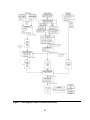
Figure 7. Flow diagram of tide correction procedures. ........................................40
Figure 8. Trafficshed definitions. .........................................................................50
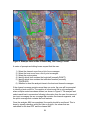
Figure 9. Example travel routes in Estero Bay, Lee County, Florida...................54
vii
viii
Abbreviations and Acronyms
AAT
AML
CIR
DGPS
DOQQ
ESRI
FDEP
FLUCCS
FMP
FSG
FTP
GICW
GIS
GPS
HDOP
JPEG
LABINS
MHHW
MHW
MLW
MLLW
MSK
MTL
NAVD88
NGS
NGVD29
NMEA
NOS
PAT
PDOP
PID
RTCM
RTL
SNR
SSF
SWFWMD
TSIP
WCIND
UF
USACE
USCG
USGS
UTC
Arc Attribute Table
Arc Macro Language
Color Infrared
Differential Global Positioning System
Digital Orthophoto Quarter Quadrangle
Environmental Systems Research Institute
Florida Department of Environmental Protection
Florida Land Use and Cover Classification System
Florida Marine Patrol
Florida Sea Grant
File Transfer Protocol
Gulf Intracoastal Waterway
Geographic Information System
Global Positioning System
Horizontal Dilution of Precision
Joint Photographic Experts Group
Land Boundary Information System
Mean Higher High Water
Mean High Water
Mean Low Water
Mean Lower Low Water
Minimum Shift Keying
Mean Tide Level
North American Vertical Datum of 1988
National Geodetic Survey
National Geodetic Vertical Datum of 1929
National Marine Electronics Association
National Ocean Service
Polygon or Point Attribute Table
Positional Dilution of Precision
Parcel Identification Number
Radio Technical Commission for Maritime Services
Raster Transfer Language
Signal-to-Noise Ratio
Standard Storage Format (Trimble Navigation, Inc.)
Southwest Florida Waterway Management District
Trimble Standard Interface Protocol
West Coast Inland Navigation District
University of Florida
U.S. Army Corps of Engineers
U.S. Coast Guard
U.S. Geological Survey
Coordinated Universal Time
ix
x
Acknowledgements
Many people have contributed to the philosophy and methods of the Regional
Waterway Management System that is embodied within this manual. We would
be remiss not to mention their contributions.
First and foremost, the combined vision and determination of Dr. Gustavo A.
Antonini, Sea Grant Professor Emeritus, and Charles Listowski, Executive
Director of the West Coast Inland Navigation District, led to the concept and
subsequent creation of the Regional Waterway Management System. The
evolution of their innovative ideas over the past 10 years has led to application of
the System in over 1000 miles of waterways in southwest Florida. Their
contributions to Coastal Management in Florida are recognized throughout the
state both by their colleagues and by state, regional, and local legislators and
coastal managers.
The counties of Sarasota, Manatee, and Lee had the foresight to apply the
Regional Waterway Management System to their coastal waters. Specific county
commissioners championed the implementation of the System within their
respective counties and provided advice: Commissioner Jack O’Neil in Sarasota
County, Commissioner Joe McClash in Manatee County, and Commissioner Ray
Judah in Lee County. Program administrators for each county were Gary Comp,
Sarasota County Natural Resources Department; Jim Englehardt, Manatee
County Human Services Division; and Steve Boutelle, Lee County Division of
Natural Resources.
The methods contained in the manual have been polished and honed by field
staff over the years. Lana Carlin-Alexander served as field crew chief for over 3
years and provided many innovative ideas and enhancements. Field technicians
who also have contributed include Patricia Knoll, Bob Williams, Ann Brock, Jerry
Gibbs, Chuck West, Jerry Wilson, Brad Stephens, Jim Givens, John Henry, and
Sharon Schulte,
Enhancements to specific methodological techniques and field survey
procedures have been provided by Cindy Fowler, NOAA Coastal Services
Center; Jack Wallace, Senior Hydrographer, National Ocean Service; Dr. Donald
Sheppard, Bill Miller, and Sydney Schofield of the University of Florida Coastal
and Oceanographic Engineering Program; Evan Brown, previously of the West
Coast Inland Navigation District; and Wanda Wooten and Bob Wasno (currently
with Florida Sea Grant) of the Lee County Division of Natural Resources.
xi
xii
Introduction
This manual details the procedures that are necessary to complete a Regional
Waterway Management System for Florida’s coastal canals and waterways. The
purpose of the Regional Waterway Management System is to provide the West
Coast Inland Navigation District (WCIND) and coastal counties with a scientific
approach that allows for boat channel maintenance while protecting resources.
The Regional Waterway Management System provides a planning tool that
permits managers and policymakers to prioritize channel maintenance needs on
a regional basis.
The Regional Waterway Management System
The methodology and objectives of the Regional Waterway Management System
stem from a pilot study (Antonini and Box 1996) conducted by Florida Sea Grant
(FSG) and the West Coast Inland Navigation District (WCIND) in Sarasota Bay.
The pilot study, designed for southwest Florida waterways, was a test application
of a management system consistent with municipal, county, Florida Department
of Environmental Protection (FDEP), and WCIND goals of facilitating safe
boating and reducing boating impacts on natural resources. The design criteria of
the Regional Waterway Management System are: (a) fit channel maintenance to
boat draft needs; (b) minimize impacts on bay habitats; (c) prioritize and evaluate
management alternatives on a regional scale; and (d) identify information
products, for boaters and shore residents, which encourage environmental
awareness by users of neighborhood waterways and boat access channels.
Results from the pilot study led to follow-up studies in south Sarasota, Manatee,
and Lee Counties (Antonini, Swett, Schulte, Fann 1998; Swett, Antonini, Schulte
1999; Swett, Fann, Antonini, Carlin Alexander 2000, 2001). Waterway
Management System results provide Florida counties with a rationale and
method for implementing a Regional Waterway Management System containing
the following elements: (a) documentation of existing depths; (b) establishment of
maintenance dredging requirements according to user draft specifications; (c)
placement of signs to conform with boat density and traffic patterns; (d)
management of boat traffic based on detailed knowledge of boat distributions
and travel routes; (e) siting of habitat restoration to protect waterways; (f)
regional scale permitting to accommodate water-dependent uses and to minimize
environmental impacts; and (g) educating the public, using waterway maps and
guide materials, to instill stewardship and best boating practices.
A Memorandum of Agreement (MOA), signed by the FDEP, FSG, and the
WCIND (September 26, 1997), provides the required, state-approved framework
for a Regional Waterway Management System that is needed to implement the
study results.
1
Waterway Management System Methods
The implementation of a Regional Waterway Management System consists of
five broad work phases, which include: 1) preparation, 2) field surveys, 3) postprocessing, 4) data analysis, and 5) development of the final products.
The preparatory phase includes such components as gathering necessary data
and map materials, hiring and training new personnel, acquiring and configuring
equipment, and determining the location and extent of waterways to be included
in a waterway management project. Boat channels are identified by interpretation
of section aerials, by field reconnaissance, and by tapping local knowledge of the
study area’s boaters; wherever present, permitted and non-permitted channel
markers are used to guide channel identification.
Two field censuses and one field survey are conducted along salt-water
accessible canals and waterways using a Differential Global Positioning System
(DGPS) to map features of interest. Geographic locations and attributes are
logged for boats; boat locations (“moorings”), whether occupied or vacant;
derelict vessels; boat-related signs; and channel centerline depths.
Post-processing includes cleaning the boat/mooring and sign census data,
cleaning the depth survey data, correcting survey depths to a standard datum,
such as the Mean Lower Low Water (MLLW) tidal datum, and transferring
property information to each boat and mooring feature.
Data analysis consists of correcting depths to MLLW using tide gauges installed
at appropriate locations throughout the project area. An ArcInfo “Arc Macro
Language” (AML) application determines channel restrictions and boat
accessibility levels from the field data.
Final products include three sets of large-scale (1:2400) map atlases, an ArcView
Map Atlas application, a CD containing primary and secondary Geographic
Information System (GIS) data layers provided in an ArcView application, and a
final report that includes a prioritization of maintenance alternatives.
2
Project Requirements
Personnel
The application of the Waterway Management System involves a wide variety of
tasks and functions. Different software packages and specialized equipment are
used during each project phase, and they require personnel with a high level of
expertise. Furthermore, during each implementation of a Regional Waterway
Management System, unique situations arise that require project personnel to
devise innovative solutions.
Fieldwork includes a bathymetric survey, a boat and mooring census, and a sign
census. All three require a vessel operator with good seamanship, navigation,
and safety skills. Field personnel should have detailed local knowledge of the
waterways within the project area. In particular, the person who conducts the
bathymetric survey should (a) be very familiar with preferred travel routes, shoal
locations, and local boating patterns and behaviors and (b) be prepared to
observe and consult boaters encountered during the survey to identify waterways
actually used. The person who conducts the boat census should have good boat
identification skills, including the ability to identify vessel types and determine
their characteristics: such as make/model, draft, and length.
Field personnel, excluding the boat operator, should have good computer skills,
or they will need to be trained. Skills required include familiarity with the
computer systems and the various software packages discussed below.
Furthermore, field personnel should have Internet familiarity, including the ability
to use e-mail and FTP in order to communicate with other project personnel. The
persons who conduct the fieldwork should have an understanding of the basic
principles of DGPS, including knowledge of the various parameters and settings
that are necessary to assure survey accuracy and quality. These will be
discussed in a subsequent section. Formal instruction in the use of DGPS, such
as the course needed to obtain Trimble DGPS operator certification, is desirable.
Computers
The number of computers required to accomplish project tasks will depend on
the scope of each particular waterway management project that is undertaken. In
general, computers will be needed for field and office personnel responsible for
processing project data. Computer related tasks associated with past waterway
management projects have been performed on desktop and laptop computers
running several versions of the Microsoft Windows operating system, including
98, NT, and 2000. The Arc Macro Language (AML) program that determines boat
accessibility levels and channel restrictions is designed to run on a Sun Solaris
system with UNIX ArcInfo. Specifications are given below for the computer
equipment used by FSG to implement waterway management projects at
publication time. In general, higher end systems should be used to implement
future projects.
3
Field operations, particularly the bathymetric survey, are accomplished using a
Rocky II+ ruggedized notebook from AMREL Systems, Inc. This notebook is
designed for field and in-vehicle applications. The laptop is certified to the MILSTD 810C and E1 standard and is rain, temperature, shock, vibration, salt fog,
and humidity resistant. Computers used for office related tasks include two
systems: 1) a Dell Dimension XPS T750r 750 MHz Pentium III with an 18GB
SCSI hard drive, and 2) a Sun Ultra II system running Solaris 2.5. Complete
specifications for project equipment are contained in the Appendix.
Software
The software programs listed below are used during various project phases.
1.
2.
3.
4.
5.
ESRI ArcInfo 8.x for Workstation
ESRI ArcInfo 7.2 for Solaris
ESRI ArcPress for Solaris
ESRI ArcView 3.x
SURVCORR and BASELINE2—tide correction programs (supplied on
accompanying CD-ROM)
6. Microsoft Excel
7. Microsoft Access
8. Microsoft Word
9. Adaptec Easy CD Creator
10. Trimble Pathfinder Office 2.51
11. Trimble Asset Survey Software
12. Trimble TSIP TALKER (version 2.0)
13. E-mail and FTP software
14. Compression software (e.g., WinZip)
Differential Global Positioning System
The Regional Waterway Management System, as designed, is intended as a
planning tool. However, the bathymetric survey procedures and methods meet
Class 1 standards as described in the U.S. Army Corps of Engineers (USACE)
Hydrographic Survey Manual (U.S. Army Corps of Engineers 2001) and
hydrographic survey specifications of the National Ocean Service (National
Ocean Service 1999).
Two code phase DGPS units are used to record horizontal positions: 1) a Trimble
Pro XR DGPS with a TSC1 data logger and a radiobeacon receiver is used for
the boat and signage censuses, and 2) a Trimble DSM212H GPS receiver with
an integrated MSK dual-channel receiver with EverestTM technology2 is used for
1
Rated for shock, vibration, temperature (operating—0o C to 50o C; storage—20o C to 60o C),
humidity (85-95% RH), rain (4 in./hr/ 0.5-4.5 mm/drop 30 min. period), salt fog (35o C 5% 48 hour
period), and altitude.
2
Everest technology improves results in high multipath environments and locations where other
radio frequencies could jam the GPS signals.
4
the bathymetric survey. Under optimum conditions, the horizontal accuracy
(RMS) for both GPS units, using the RTCM radiobeacon transmissions, is 50 cm
+ 1 ppm on a second-by-second basis, which, for the 4-county area of the
WCIND, is better than 1 meter (Trimble Navigation Ltd. 1998b). Under normal
operating conditions the horizontal accuracy for 95 percent of feature positions is
expected to be 2 meters or less, which conforms with USACE and National
Ocean Service (NOS) accuracy standards. An Advantage Range Finder from
Laser Atlanta measures feature offsets during the boat and sign censuses.
Survey Vessel
In order to provide background on suitable vessel types needed to complete
fieldwork, a description of vessels used during recent projects follows. The first
vessel, a Key West model 1720, is an open fisherman with a shallow V fiberglass
hull and a center console. The Key West has a 70hp, 4-stroke, Evinrude
outboard and a fuel capacity of 31 gallons. The second vessel, a Boston Whaler
130 Sport, is an open sport with a side console and a tri-V fiberglass hull. The
Whaler has a 25hp, 4-stroke, Mercury outboard and a fuel capacity of 6.6
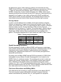
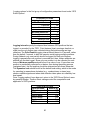
gallons. The physical characteristics of each vessel are found in Table 1 below.
Table 1. Survey vessel parameters.
Length
Beam
Weight (lb)
Draft
Key West
17’ 2”
6’ 10”
1050
8”
Boston Whaler
13’ 3”
5’ 11”
600
7”
Depth Sounding Equipment
Sounding equipment consists of a Bathy-500MF multi-frequency, single-beam
echo sounder (Ocean Data Equipment Corporation); a Standard Horizon DS150
single-beam echo sounder (Standard Communications); and a fiberglass
sounding pole, calibrated and marked at 0.01-foot intervals (see Appendix for
equipment specifications).
Soundings from the Bathy-500MF and the DS150 are passed to HYPACK Max
hydrographic survey software (Coastal Oceanographics, Inc.) loaded on the
AMREL Rocky II+ notebook computer. The sounding pole is used to verify any
suspect echo sounder readings and to check depths in shallow areas (below 3
feet). Calibration of the depth sounders is accomplished using a bar, which
consists of a 1.25 ft. X 2.9 ft. lead-weighted aluminum plate. The bar is lowered
below the transducer with a 25-foot long, 1/8-inch diameter twisted stainless steel
wire cable marked at 5-foot intervals, from 5 feet to 20 feet.
Tide Level Recorders and Stilling Wells
Tide observations are necessary to correct soundings to chart datum (MLLW).
Tide level recorders consist of Model 220 solid-state, ultrasonic fluid level
sensors manufactured by Infinities USA, Inc. (see Appendix for equipment
5
specifications). Each Model 220 data logger stores 3,906 records, which allows
for 16 days of tide data at a logging interval of 6 minutes. Data files can be
downloaded, in the field, to a laptop computer or an HP-48GX calculator and
examined for integrity.
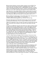
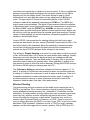
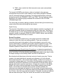
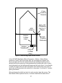
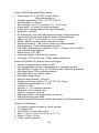
Each gauge is mounted on a stilling well, the dimensions of which are shown in
Figure 1. All sections of the stilling well are cemented together except for the cap,
which is secured to the closet flange using two padlocks to protect the tide level
recorder. The stilling well is secured to a piling using wooden I-beam mounts and
stainless steel worm gear clamps.
Data Products
Several GIS data themes need to be obtained or created during the preparatory
phases of the waterway management project. These data sets must meet project
currency requirements and they must cover the geographic extent of the project
area. Required data include background imagery, existing USACE bathymetric
surveys, seagrass and mangrove coverages, salt-water accessible parcel
boundaries and attribute information (parcel identification number, owner, and
address), and vertical benchmark locations and attributes. Each data set is
described below.
The Albers equal-area3 projection is the recommended projection system for the
waterway management project. At present, most third-party data sets necessary
to complete the project are distributed in this format. Table 2 lists the projection
parameters.
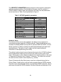
Table 2: GIS data projection parameters.
Projection Parameters
Albers
Projection
Meters
Units
HPGN (or NAD83)
Datum
240 00’ 00’
1st standard parallel
310 30’ 00”
2nd standard parallel
-840 00’ 00”
Central Meridian
240 00’ 00”
Latitude of projection's origin
400000.0
False easting (meters)
0.0
False northing (meters)
3
Equal-area means that a spatial unit of set size, when placed on different parts of a map, will
cover exactly an equal area of the actual earth, no matter where on the map the unit is placed.
Although neither shape nor linear scale is truly correct, the distortion of these properties is
minimized in the region between the standard parallels.
6
Figure 1. Stilling well schematic.
7
U.S. Geological Survey (USGS) Digital Orthophoto Quarter Quadrangles
(DOQQs) are recommended for use as background imagery during all project
phases. This imagery is readily available for all areas of Florida and can be
obtained in JPEG image compression format, at resolutions of 1, 2, and 3-meter,
from the web site maintained by the Land Boundary Information System
(www.labins.org).
DOQQs combine the image characteristics of a photograph with the geometric
qualities of a map. Image displacements caused by camera tilt and terrain relief
are removed, so that ground features are displayed in their true ground position.
This allows for the direct measurement of distance, areas, angles, and positions.
Furthermore, a DOQQ displays features that may be omitted or generalized on
maps. The DOQQs used for past waterway management projects in southwest
Florida are based on 1994-95, 1:40,000-scale Color Infrared4 (CIR) photography.
USACE bathymetric surveys have been used during past projects to complement
data collected by FSG or to provide data for areas not surveyed by FSG, such as
the Gulf Intracoastal Waterway (GICW). A point of contact, to determine the
availability and characteristics of USACE survey data, is the ConstructionOperations Division of the Operations and Maintenance Technical Support
Section of the USACE (904-232-1132; P.O. Box 4970, Jacksonville, FL 322320019).
Seagrass, mangroves, and land use/land cover normally are extracted from
databases obtained from third parties, such as Florida’s Water Management
Districts. For example, the Southwest Florida Waterway Management District
(SWFWMD) has ArcView shapefiles of seagrass for the years 1982, ‘88, ‘90, ‘92,
‘94, ’96, and ‘99. The seagrass beds were interpreted from 1:24,000 natural color
aerial photography. The spatial extent of the SWFWMD seagrass GIS databases
varies from year to year, but generally extends from Tampa Bay to Charlotte
Harbor.
Mangroves normally are extracted from a land use/land cover GIS database that
is categorized according to the Florida Land Use and Cover Classification
System (FLUCCS) (Florida Bureau of Comprehensive Planning, 1976) and
whose features were photo-interpreted from 1:12,000 USGS CIR DOQQs.
SWFWMD GIS databases are available for download from:
www.swfwmd.state.fl.us
Parcel boundaries and property appraiser data may be obtained from the
appropriate local or regional agency. Ideally, parcel boundaries are available as
ArcView polygon shapefiles in the Albers projection. If not, they will need to be
converted to a shapefile and re-projected. The parcel boundary GIS file should
contain the parcel identification number (PID) in the theme attribute table. The
4
Color infrared photography differs from conventional color film because its emulsion layers are
sensitive to green, red, and near-infrared radiation (0.5 micrometers to 0.9 micrometers).
8
PID enables linkage of the parcel boundary file to information contained in the
property appraiser database. Property appraiser data should be obtained for the
parcels within the study area and fields should include parcel owner name and
address.
Vertical benchmark information is obtained from several sources, starting with
local offices of city and county surveyors. A number of web sites maintained by
state and federal agencies contain detailed benchmark information. The LABINS
web site (www.labins.org) contains databases with information on horizontal and
vertical benchmarks, including the National Geodetic Survey (NGS) database
and USGS 3rd order vertical data. The National Ocean Service (NOS)
(www.ngs.noaa.gov/datasheet.html) allows retrieval of NGS data and NOS tidal
benchmark information via interactive map, permanent identifier, radial or
rectangular search, station name, project identifier, or USGS quad name. USGS
tide gauges and associated benchmarks are situated in a number of locations
throughout the state and their location and status is recorded in the USGS Water
Year reports. Contact the USGS to determine their availability and suitability for
project requirements.
9
10
Project Planning and Preparation
Project Planning Map
The field crew requires a map of the study area that delineates the salt-wateraccessible canals, channels, and other waterways where boats, moorings,
derelict vessels, and signs are to be tallied and where depths are to be surveyed.
A copy of the map should be made for each field census and survey to help plan
and monitor fieldwork progress. For past waterway projects USGS 1-meter
DOQQs were used as the map base. Map production is best accomplished in
GIS software, such as ArcView. A permanent ArcView Project file should be
created so that future modifications or additions can be readily incorporated.
The planning map includes several GIS themes, most importantly the location
and extent of channel centerlines throughout the study area. The overview
provided by the planning map will help to plan the work schedule, monitor field
progress, and annotate areas as they are completed. As each segment of
fieldwork is completed, the resulting data should be mapped in the GIS to ensure
that no data gaps exist.
The planned waterway centerlines are best drawn by persons with knowledge of
travel routes actually used by boaters. The county or regional agency that is
charged with waterway management within the project area should oversee this
procedure. For example, during project implementation in Lee County, personnel
from the Marine Services Program, a section of the Division of Natural
Resources, determined the extent and location of channels to be included. The
resultant map is deemed preliminary, as the field crew will update it during the
surveys. Field personnel should, as necessary, consult knowledgeable shore
residents and observe actual boat travel routes.
Other themes included on the planning map are the locations and characteristics
of signs, vertical benchmarks, hydrologic areas, tide gauges, locks, boat lifts, etc.
Depending on project circumstances, additional map themes may be helpful. The
sign census is conducted first and the resulting GIS theme included on the
planning map for the depth survey. Vertical benchmarks can be categorized by
their source, such as marks from the city or county, LABINS, NOS, or USACE.
Hydrologic areas are delineations drawn by project personnel to guide the
placement of tide gauges and the scheduling of depth survey work. Their
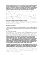
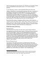
inclusion on the planning map is important in complex areas, as exemplified by
the City of Cape Coral (Figure 2). In less complex situations, hydrologic areas
may be unnecessary. The map should include planned tide gauge sites (see Tide
Gauge Siting) and gauges that are maintained by other agencies, such as the
USGS.
11
Figure 2. Hydrologic areas.
Tide Gauge Siting
During collection of bathymetric data, the water surface elevation relative to
mean lower low water (MLLW) will vary with local tides, freshwater flows, and
environmental effects (e.g., wind). To correct for these effects, all bathymetric
data are collected near a gauge or between pairs of gauges. Gauge sites are
selected in accordance with NOS and USACE standards required for tidal
correction of bathymetric data (National Ocean Service 1999; U.S. Army Corps of
Engineers 2001). The spatial distribution of project tide gauges is determined in
consultation with qualified personnel5 using the mapped hydrologic areas to
guide gauge siting. Additional factors considered for gauge locations include
safe, secure sites, and the availability of nearby monuments of known elevation,
to which gauges can be referenced.
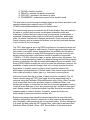
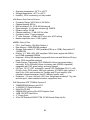
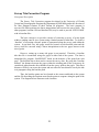
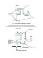
Survey Vessel Outfitting
Survey equipment needs to be securely mounted on the vessel before initiating
fieldwork (Figure 3). The exact location that equipment is mounted will depend on
the particular vessel used for the survey and on the positioning of personnel
during the survey. Though the survey equipment, which was described
previously, is designed for foul weather conditions, precautions should be taken
to protect the equipment from inclement weather and salt spray.
5
Dr. D. Max Sheppard, Professor in the University of Florida Coastal and Oceanographic
Engineering Program, provided guidance on tide gauge siting in several study areas.
12
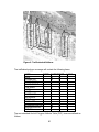
Currently, a 17-foot Key West is used for the bathymetric survey (Figure 3G). An
explanation follows on how the equipment was mounted on the Key West, in
order to guide the placement of sounding equipment on other vessels. A special
side mount for the Bathy-500MF transducer fits in a rod holder on either the port
or starboard side (Figure 3A). The DGPS antenna is attached directly above the
transducer mount and, thus, directly over the Bathy-500MF transducer (Figure
3A and C). A bulkhead mount holds the Bathy-500MF instrument on the inside,
forward, port side (Figure 3D); a custom fabric cover protects the Bathy-500MF
from spray. The DSM212H DGPS is mounted on the inside back cover of the
Bathy-500MF. The Horizon DS150 transducer is transom mounted and the
DS150 display unit is placed on the console, visible to the boat operator. A
fighting chair for the equipment operator, forward of the console, replaces the
original passenger seat cushion (Figure 3E). A swivel mount, adapted from a
commercial monitor stand, holds the AMREL laptop forward of the chair (Figure
3B). This mount is bolted to the aft bulkhead of the foredeck. A custom canvas
dodger, with a roll-up clear plastic forward window, protects the entire work area
from spray and rain and provides shade that improves the laptop computer
display visibility (Figure 3G).
Two custom 12V outlets, in addition to the cigar lighter on the console, provide
power for the survey equipment. A dual-battery system, with a second battery
added in parallel with the original boat battery, has proven a reliable source of
clean instrument power.
The Trimble Pro XR DGPS, the TSC1 data logger, a radiobeacon receiver, and
the Laser Atlanta rangefinder are used for the boat/mooring and sign censuses.
The census taker sits in the captain’s chair, adjacent to the DGPS antenna,
which is mounted in a rod holder.
A maintenance schedule needs to be established and followed for each of the
survey vessels. Each day the vessel should be secured and all survey equipment
removed. During the bathymetric survey, it is important that fuel be kept within a
certain range to insure that the load conditions do not vary from one extreme to
another, thus affecting the static draft.
In order to minimize travel time, suitable locations to overnight the boat should be
found. This will require locating willing local residents. Likewise local residents
with appropriate facilities should be found for mounting tide gauges on docks. (A
productive way to find such volunteer participants is through organizations such
as boating clubs.) Key site criteria include security for the boat and tide gauges,
as well as accessibility by the field personnel. Prior permission must be obtained
to access the tide gauge or use the dock when no one is home.
13
Figure 3. Bathymetric survey equipment.
14
Field Procedures
Tide Gauge Installation
Once appropriate tide gauge sites are established (see Tide Gauge Siting),
secure facilities need be found where gauges can be installed. Experience has
shown that the best location is a dock at a private residence, as it provides
greater security. Each proposed gauge site should be visited to confirm the
presence of vertical benchmarks and their suitability to determine tide gauge
elevation. Ideally, benchmarks are located within sight of the tide gauge
installation, such as on a seawall or on an adjacent road or structure. If no
suitable benchmarks are found in the vicinity of the gauge site, then a licensed
surveyor must establish benchmark (at least 3rd order), or another gauge site
needs to be selected.
Naturally, property owners must give permission to install gauges on their docks.
Tide gauge stilling wells must be securely fastened to a protected piling or other
suitable mounting location (Figure 3F). Stainless steel straps, similar to
automotive hose clamps, but available in lengths of 4 feet or longer, have proven
a satisfactory means. Straps with thread slots over most of their length, rather
than just near the tip, are preferable, as they accommodate a wide variety of
dock piling diameters. An I-beam of 2 x 4 lumber, securely screwed together and
placed between the stilling well and piling, provides a stable mount with a
suitable standoff distance. The field crew must carefully monitor the gauge’s
elevation relative to the piling to check for vertical slippage or other problems.
The elevation of installed gauges, relative to NGVD29 or NAVD88, can be
determined by differential leveling conducted by project personnel. If the
benchmark is located on a seawall, then simultaneous measurements to the
water surface from both the gauge and benchmark are used to establish gauge
elevation. The average of three or more measurements, made under calm
conditions, is used to establish the gauge elevation. From other benchmarks, not
located on seawalls, the gauge elevation can be established via differential
leveling. The MLLW tidal datum is determined in reference to historical NOS tidal
benchmarks located in the vicinity of the gauge. The NOS tidal benchmark
sheets, in many cases, provide elevations of tidal and geodetic datums
referenced to MLLW (feet). The following example is for a historical NOS tide
gauge that was located on the Peace River:
15
HIGHEST OBSERVED WATER LEVEL
MEAN HIGHER HIGH WATER (MHHW)
MEAN HIGH WATER (MHW)
MEAN TIDE LEVEL (MTL)
* NATIONAL GEODETIC VERTICAL DATUM-1929 (NGVD)
MEAN LOW WATER (MLW)
MEAN LOWER LOW WATER (MLLW)
LOWEST OBSERVED WATER LEVEL (01/16/1972)
=
=
=
=
=
=
=
=
3.85
2.24
1.93
1.17
0.56
0.41
0.00
-2.72
Tidal benchmark sheets may be obtained from the following NOAA web site:
http://co-ops.nos.noaa.gov/bench.html. Supplemental water level data may be
obtained from USGS water-stage recorders when located within project areas.
During installation of the tide gauge, record all critical parameters on the ‘Gauge
Installation Form’, which can be found on the accompanying CD-ROM
(/FieldProcedures/TideGaugeInstallationForm.doc). Information recorded on this
sheet includes benchmark characteristics and a record of the procedures and
measurements obtained during tide gauge calibration and leveling procedures.
This information is of vital importance when correcting depth measurements to
the MLLW tidal datum.
Tide corrections are performed by means of a computer program, Survey Tide
Correction (SURVCORR.exe), developed by the University of Florida (UF)
Coastal and Oceanographic Engineering program. SURVCORR was developed
to correct depths within a winding canal or river system. The program, with inputs
of spatially referenced soundings and tide gauge readings, determines and
applies depth corrections based on time and relative location. Tide data are
interpolated to each centerline, or user-constructed baseline point, by assuming
a linear variation of the tide through the system. Weighting the interpolation by
the distance from a gauge provides correction for non-linear effects, such as
viscous dissipation. A more detailed description of the program can be found in
the Appendix (see Survey Tide Correction Program).
Setting the Tide Gauge Data Logger
After the tide gauge stilling well is secured in its operating position and nearby
benchmarks identified to serve as elevation references, set (program) the data
logger, in accordance with the Infinities user manual (Infinities USA, Inc. 1999).
The logger can be set using either a laptop computer or a Hewlett–Packard
HP48GX calculator. A laptop PC is faster, and its software is considerably more
user–friendly. However, the HP48GX is much handier in the field and is usually
the interface device of choice. The following paragraphs summarize the
procedure for setting a data logger with the hand–held calculator.
16
Before beginning fieldwork, load the Infinities software into the HP48GX. The
Infinities user manual explains this rather complicated process in detail. For
step–by–step help, call Infinities USA at 1-888-808-5488. (Important: A special
version of the Infinities data logger software, included on the accompanying CD,
allows use of the “Offset” field to tag a site–specific numeric identifier code to
each data record. If the standard Infinities software is used instead, the numeric
value of the code entered will be added to each record! The site code will stay
the same until the logger is reset at a different site.) Set the calculator’s internal
clock. (Experience has shown it advisable to set all system clocks to UTC.)
Before installing the special version of the Infinities data logger, decompress the
three disk images on the CD-ROM to 3-1/2 inch floppies
(/FieldProcedures/InfinityGauge/Disk1.zip, Disk2.zip, and Disk3.zip).
Setting the data logger and downloading data are done via the HP serial cable
purchased with the calculator. First, turn on the HP48GX and then insert the
cable into the calculator’s top 4–pin socket. Be careful; the socket pins are easily
bent. Connect the 9–pin connector on the other end of the cable to the data
logger.
Navigating the HP48GX’s keyboard is best done at first with the Infinities manual
on hand, as each key has multiple functions. To set the data logger, select Set
Datalogger from the Datalogger Start Menu and then choose Reset Auto Set.
Enter a three–digit identifier code number for the station and press the OK “soft
key” (the key below the desired choice in the calculator’s display). It is best to
enter the station codes for a study area with large numbers, such as 100, 101,
etc., rather than 001. Then, if an HP48GX with the standard Infinities software is
inadvertently used, and the code is added to the depth readings as an “offset,”
the large resulting error will be immediately obvious.
The Time to Begin display will appear. Enter the number of days (zero), hours,
minutes, and seconds (zero) from 12AM to the desired first sounding time. For a
6-minute logging interval, choose to start at 0, 6, 12, 18…or 54 minutes after the
hour. (The software uses a 24-hour clock system.) As an example, if the present
time is 3:08PM, enter zero days, 15 hours, 12 minutes, and zero seconds to start
the logger at 3:12PM (1512 in the 24–hour system), the next appropriate logging
time for a 6–minute interval. Press OK when the setting is correct, and enter the
Time Interval Between Readings in hours (zero), minutes (6), and seconds
(zero). Press OK to return to the Datalogger Start Menu.
Make several data logger readings and nearly simultaneous staff gauge or tape
measure determinations of drop to the water surface from the stilling well rim
(which corresponds to the logger’s transducer height). This can be done by
waiting for the logger to make its scheduled readings every six minutes. A more
efficient method is to select Current Status from the Datalogger Start Menu,
which will cause the logger to immediately take and display a reading. (This
special reading is not stored in the logger memory, so it will not appear in
downloaded data files.) Record and compare the readings. If the logger sounding
17
error exceeds the specified limit (1 percent of reading), calibrate the logger, using
the logger’s built-in calibration routine, and then repeat the measurements. To
calibrate the logger, select Calibrate Logger from the Datalogger Start Menu and
enter a depth reading and its corresponding manual measurement. Then take a
couple of additional test readings to verify the calibration reduced the error to
within the specification.
Scroll down to Name & Message on the Datalogger Start Menu to enter a name
for the station (8 characters maximum) and, if desired, additional text (up to 31
characters). This information will appear in the headers of downloaded data files,
but—unlike the three–digit numeric station code entered earlier—it is not tagged
to each data record.
When the data logger is correctly programmed, wait for a least one scheduled
reading to be taken, and download it as described in the next section. If the
reading is on time and appears reasonable, the logger is running and collecting
water level data. Screw the data logger’s cap on snugly and install the protective
housing on the stilling well assembly.
Be sure to record the drop from the chosen benchmark to the water
simultaneously with some of the readings taken after the gauge is calibrated and
known to be taking accurate readings. That information will later be used in
adjusting the data logger’s water level readings to a tidal datum (such as mean
lower low water).
Download Data Files
Each tide station data logger should be downloaded at least weekly, preferably
more often, in order to ensure data are not lost due to “wrapping,” which occurs
when the logger’s memory is full and each new record causes deletion of the
oldest record in storage. Also, frequent visits to a tide station will reveal problems
(malfunctions, stilling well movement, theft, vandalism, etc.) before many days of
soundings are taken that can not be corrected for tides.
Connect the HP48GX to the data logger as described above. From the
Datalogger Start Menu, choose a data dump mode. Dump Since Set, which
downloads all data collected since the logger was last set, is the usual choice.
(An Entire Memory Dump downloads all data in the logger. If there is any doubt
about whether data have been downloaded and backed up, the Entire Memory
Dump will collect all possible readings. Then the station-unique ID number will
allow sorting out which records came from which site.) When a mode is selected
and OK pressed, the data will be transferred from the logger to the HP48GX.
Examining a plot of the data allows a quick data quality check. From the
Datalogger Start Menu, select View Plots, and then scroll to select a file to view.
The newest file will be at the top of the list. If the data are good, the plot will
clearly show the rise and fall of the tide. The small screen shows a limited subset
(“page”) of the data at a time. Pressing the Cancel soft key will display the next
pages until the file has been completely viewed. Press the (X,Y) soft key to show
cursor coordinates, then move the cursor via the arrow keys to some data points
18
near the top and bottom of the plot. This allows verifying the displayed tide range
is reasonable. Units are inches. (If the stilling well bottom aperture is partially
blocked or the pressure relief hole is completely obstructed, the water level in the
well may rise and fall with the tide, but with amplitude less than the actual tidal
variation.) Press Cancel to exit View Plots and then Enter to return to the
Datalogger Start Menu. When the data dump is complete, the logger will continue
to collect depth readings.
Transfer Files to a PC
Back in the office, connect the HP48GX calculator to a serial port on a Windows
computer, using the same HP serial cable used with the data loggers. Start the
Infinities PC Transfer 95 98 NT program and select Handheld Retrieval Device.
Choose the serial port to which the HP calculator is connected and then click
Receive Files. Status bars show the progress of the download. The HP48GX
shuts itself off when it is finished sending all of its files.
The downloaded files can be immediately inspected in a text or word processor
or opened as delimited text files in a spreadsheet, for graphing or preparation of
files for tidal correction of soundings.
Equipment Settings
The following sections cover the principal settings for project equipment. Before
using any piece of equipment, carefully read its accompanying user/operational
manual.
GPS Parameter Settings
The Trimble Pro XR, TSC1 data logger, and the MSK beacon receiver are used
for the boat/mooring and sign censuses; the Trimble DSM212H is used for the
depth survey. Feature positional accuracy obtained during data collection
depends on several factors including the number of satellites, multipath, distance
between base station and the rover, Positional Dilution of Precision (PDOP),
Signal-to-Noise Ratio (SNR), and satellite elevation (Trimble Navigation Ltd.
1995). These factors may be controlled or monitored via software and hardware
settings. The following discussion describes parameter settings for field data
collection during the waterway management project. A more detailed discussion
of each parameter may be found in the Trimble manuals that accompany the
GPS equipment (Trimble Navigation Limited 1998a, 1998b, 1998c).
The Asset Surveyor software on the TSC1 data logger is used to set critical and
non-critical parameters for data collection (Trimble Navigation Limited 1998a). As
fieldwork progresses all settings should be confirmed daily, as they have been
known to occasionally reset to their default values. Parameter settings are
accessed from the ‘Configuration’ menu, which is one of eight selections found
on the Asset Surveyor main menu. The following paragraphs discuss appropriate
settings for each relevant parameter, which are displayed in bold italics in the
tables that accompany the discussion.
19
‘Logging options’ is the first group of configuration parameters found under ‘GPS
Rover Options’.
LOGGING OPTIONS
Logging intervals
Point Feature:
5s
Line/area:
6s
Not in feature:
None
Velocity:
None
Minimum positions:
1
Carrier phase
Carrier mode:
Off
Minimum time: 10 mins
Dynamics code:
Land
Logging intervals specify the elapsed time between GPS positions that are
logged, or recorded, by the TSC1. Point features (boat, moorings, derelicts, or
signs) are the only feature type collected during the boat/mooring and sign
censuses. The Point Feature logging interval should be set to 5 seconds, rather
than the default 1 second, to help the operator avoid logging multiple positions.
During fieldwork only one position should be logged for each point feature;
logging is paused after one position is recorded and, then, feature attributes are
entered into the data logger. Since only one position is to be collected for each
feature, Minimum positions should be set to a value of one. If more than one
position is accidentally collected for a feature, then during the editing process
(explained later), the first position should be retained and all others discarded.
The Dynamics code should be left at the default land setting, which is the mode
for operating in areas where obstacles (e.g., condominiums or trees) may
obscure satellite signals and when data collection takes place at a relatively low
boat speed.
Once ‘Logging options’ have been set, return to the ‘GPS Rover Options’ menu
by pressing Escape. ‘Position filters’ settings control the computation and
application of GPS positions.
POSITION FILTERS
Position mode:
Manual 3D
Elevation mask:
15o
SNR mask:
6.0
PDOP mask:
6.0
PDOP switch:
8.0
Apply real-time:
Yes
RTK mode:
Off
20
The Position mode is a critical setting, since it affects the operation of the
Trimble Pro XR GPS receiver. This parameter should be set to Manual 3D, which
assures that the receiver uses four or more satellites to compute positions. This
setting usually will yield the most accurate GPS positions and allows for greater
flexibility during fieldwork. The Elevation mask is set so that only satellites that
are 15 degrees above the horizon are used to calculate positions. This is to
assure that the same satellites used by the U.S. Coast Guard (USCG)
radiobeacon6 station are those used during fieldwork. Also, this setting helps to
avoid the greater ionospheric noise that is associated with low horizon satellites.
The Signal-to-Noise Ratio (SNR) mask compares the information content and
the noise7 that are carried by a satellite signal. Increasing values indicate that the
signal carries a relatively greater amount of information than noise; a value of 6.0
is the appropriate SNR setting. PDOP mask determines the maximum Positional
Dilution of Precision allowed to compute GPS positions. PDOP is a measure of
the quality of the spatial arrangement of the constellation of satellites that have
been acquired by the DGPS receiver. The accuracy of GPS positions increases
as the PDOP value decreases. A PDOP of 6.0 provides for sub-meter accuracy
when using a Trimble Pro XR receiver. Use the Pathfinder Office Quick Plan
utility to determine when acceptable PDOP will be available during a particular
survey day (see Mission Planning). The Apply Real-time switch should be set to
yes, since all GPS positions are to be corrected using the RTCM signal.
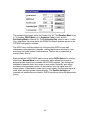
The next parameters to check are the ‘Communications options’ located under
the ‘Configuration’ menu.
REAL-TIME INPUT OPTIONS
Radio type:
Custom
Baud rate:
9600
Data bits:
8
Stop bits:
1
Parity:
None
RTCM options
Station:
Any
Age limit:
20s
6
The U.S. Coast Guard established a network of radio-broadcast DGPS stations that cover the
Pacific, Atlantic and Gulf coastlines of the U.S. plus some inland waterways. These sites
broadcast RTCM-104 v. 2 format corrections utilizing Minimum Shift Keying (MSK) modulation of
existing radio beacon signals. Each station has a broadcast range of generally 100 to 150 miles
and their data can be utilized by any MSK beacon receiver, such as the Trimble Pro XR receiver,
which has a with built-in MSK receiver. Real-time DGPS correction accuracy is specified by the
Coast Guard to be better than 10 meters. Actual field accuracies have been found to be as good
as 1 meter with a system such as Trimble's Pro XR.
7
Choose a location for the antenna with a minimal amount of ambient noise. Some common
sources of electrical and magnetic noise are gasoline engines, television and PC monitors,
alternators and generators, electric motors, propeller shafts, equipment with DC-to-AC
converters, florescent lights, power lines, and switching power supplies.
21
Real-time corrections are obtained from the radiobeacon component of the Pro
XR and, thus, the parameters should be left as listed in the table above. The
RTCM Station option is set to ‘Any’, which allows the receiver to acquire the best
signal from available USCG radio-broadcast DGPS stations. USCG DGPS
stations in Florida are located at Cape Canaveral, Key West, MacDill Air Force
Base (Tampa), and Miami. The operational parameters and current status of all
USCG radio-broadcast DGPS stations can be obtained at the following web site:
http://www.navcen.uscg.gov/ADO/DgpsSelectStatus.asp
Since the Pro XR integrated DGPS is used to apply real-time corrections, press
the F1 soft-key on the TSCI keypad in order to check the parameter settings.
INTEGRATED DGPS
Source:
Beacon
Mode:
Auto range
Frequency:
N/A
The Source for real-time position corrections is RTCM messages broadcast from
one of the USGS MSK radiobeacon stations listed above. Mode is set to Auto
range, which allows the Pro XR to track available stations and select the best
one in terms of proximity and signal strength. Frequency is not applicable since
the Pro XR is set to switch between available stations.
Return to the ‘Configuration menu’ by pressing the Escape key. The settings
under ‘Coordinate system’ and ‘Units and display’ can be left at their default
values as listed in the TSC1 Asset Surveyor Software User Guide (Trimble
Navigation Ltd. 1998a). The ‘Time and date’ settings are for TSC1 display and
file naming purposes only. GPS data is recorded in GPS time, which is
essentially the same as Universal Time Code (UTC). Thus, there will be no effect
on GPS data records if you reconfigure the receiver and/or data logger when
there is a change in the local time.
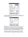
Next, from the ‘Configuration menu’, select ‘External sensors’ and highlight the
selection for Laser and press the setup soft key.
LASER RANGEFINDER
Type:
Atlanta Advantage
Auto connect:
Yes
Serial port:
Top
The laser Type should be set to Atlanta Advantage and Auto connect set to
‘Yes’, since the range finder is used throughout both censuses. The rangefinder
is connected to the top Serial port on the TSC1.
22
The last available selection from the ‘Configuration menu’, ‘Hardware (TSC1)’,
contains useful information and settings.
HARDWARE (TSC1)
LCD contrast:
30%
Backlight:
Off
Auto shutoff:
20
Beep volume:
High
Free space:
1648kB
PC card free space:
N/A
Battery source:
External
Internal battery:
100%
External battery:
Unknown
Software version:
4.01
Lighting conditions change throughout the day and LCD contrast allows the
TSC1 display screen to be adjusted accordingly. In general, with brighter lighting
a higher value is required. It is best to leave the Backlight Off, as it places a
relatively large drain on battery power. Auto shutoff powers down the TSC1
when no key has been pressed during the allotted time. Choose a setting
between 1 to 60 minutes that best meets the data entry habits of field personnel.
Beep volume set to ‘High’ will alert the user when certain data logger functions
have been performed (e.g., position recorded). The remaining fields cannot be
set, but offer important information to the user. Free space indicates how much
TSC1 storage space is left for data (rover) files. Battery source indicates
whether the TSC1 is running on its own internal batteries or from an external
power source, such as the GPS receiver battery. Internal battery indicates the
level of charge remaining in the TSC1’s main internal batteries. When the TSC1
is hooked up to an external source the External battery field shows the power
level, if available. The Software version of the Asset Surveyor software is also
displayed. This concludes the discussion of settings for the Trimble Pro XR GPS.
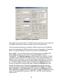
The Trimble DSM212H and its integrated dual-channel MSK beacon receiver are
configured using Trimble Standard Interface Protocol (TSIP) TALKER software
installed on a PC (e.g., the AMREL laptop, which is used during the depth
survey). The TSIP TALKER software is used to configure key GPS operating
parameters: DGPS input and output, and NMEA-0183 output messages; as well
as to monitor the current status of receiver processes. The DSM212H is
connected to a PC serial port via Port B on the DGPS. The communication
parameters are set using the TSIP TALKER software.
Once communication is established between the TSIP TALKER software and the
DSM212H, DGPS receiver parameters are accessed from the drop-down menu.
23
The settings are the same as for the Trimble Pro XR. The Elevation Mask is set
to 15 degrees, PDOP Mask to 6.0, Dynamics Code to land, and the
Positioning Mode to Manual 3D. The Positioning Rate, which is set to 1 Hertz
(Hz), determines the rate at which the DSM212H outputs position reports to the
HYPACK hydrographic software.
The DGPS menu includes options for configuring the DGPS source and
radiobeacon data acquisition channels, viewing radiobeacon information, and
monitoring the health status of radiobeacons. The first set of parameters is
located under ‘Source’.
Radio-broadcast USCG DGPS stations serve as the DGPS Source for position
corrections. Beacon Mode is set to automatic, which allows the receiver to
acquire the best signal from available USCG DGPS stations. Two settings are
available for beacon mode: auto range or auto power. Generally, auto range
provides a more accurate position, as the receiver uses the signal from the
closest station. When beacon mode is set to auto power, the strongest signal is
used, which provides greater signal reliability. The Satellite Settings are
irrelevant, as satellites are not used for DGPS corrections during the bathymetric
survey.
24
The next set of parameters located under the DGPS menu ‘Configuration’ set the
DGPS acquisition mode, the maximum pseudorange correction (PRC) age, and
the source of DGPS corrections.
DGPS Mode determines receiver behavior when DGPS corrections are received
from a radiobeacon station. Set the mode to ‘On’ to assure that the receiver
computes positions only when DGPS corrections are available. Set Max PRC
Age to 20 seconds to eliminate older PRCs from position calculations, since they
quickly age and lose accuracy. Set the External DGPS Source to ‘Any Station’
to automatically acquire DGPS corrections from any radiobeacon in the area.
The ‘Beacon List’ and ‘Beacon Health’ selections available from the ‘DGPS’
menu provide information on the available radiobeacon stations, including their
status. The ‘View’ menu lets you display windows containing status information
25
collected from the receiver. These are useful for viewing receiver configuration
and monitoring receiver processes during the bathymetric survey.
Depth Sounders
Bathy-500MF—the Bathy-500MF echo sounder is controlled using the 16 keys
that are located on the front panel (Figure 4). The settings described below are
those that have been found appropriate during a hydrographic survey conducted
for the WCIND along the Caloosahatchee River and adjoining canals and
waterways. The settings for other locations may be different. Only digital depth
output has been used during WCIND surveys; not the paper chart capabilities of
the sounder. Refer to the user manual for a complete description of Bathy-500MF
functions and parameter settings (Coastal Oceanographics, Inc. n.d.).
RANGE
DEPTH
DATA
GAIN
SV
GATE
CHART
MARK
ALARM
FEET
MTRS
PWR
OFFSET
COM
ENTER
Figure 4. Bathy-500MF echo sounder front panel.
To power up the Bathy-500MF, simultaneously depress the PWR and ENTER
keys. During the startup, view the LCD display to determine if the unit is set to
the proper transducer frequency (currently using a 200 kHz transducer). If the
transducer frequency is not properly set, then quickly press the COM key and
select the proper transducer frequency (e.g. 200 kHz) from the ‘SET FREQ’
menu.
The RANGE setting will depend on the range of depths encountered during a
particular survey. A setting of either 0—30 ft (or 0—60 ft) is normal for surveys
conducted for the WCIND. The PHASE setting is 0—120 ft, the GAIN is set to
‘Auto’, and TVG set to 100. The daily bar check is used to determine if any
26
corrections are needed due to variations in sound velocity. If there is a difference
between the sounder depth reading and the bar depth, sound velocity (SV) is
adjusted until the two depths match. Field notes should be kept to record
observations from each daily bar check and any adjustments to SV that are
made. The data output I/O format for transmitting depths to the HYPACK
software is selected by repeatedly depressing the COM key. The NMEA dbs
output format is recommended. The depth of the transducer below the waterline
is determined under normal load conditions and the measurement is entered into
the Bathy-500MF using the OFFSET key. ALARMs can be set to notify the
operator when sounder readings are above or below specified limits. Alarms can
be useful to notify the operator when the sounder gives false readings. Potential
causes of false readings can include turbulence, temperature gradients, density
variations, and biological layers.
Horizon DS150—the procedures for entering settings into the Horizon echo
sounder are described in the user manual (Standard Communications 2001). The
keel offset (depth of the transducer below the waterline) is determined under
normal load conditions (equipment and personnel) and the measurement is
entered into the HYPACK Hardware driver settings for the Horizon.
The setting for Display Damping is to control for rough water conditions, schools
of fish, and thermal layers, all of which can cause erratic depth readings. Display
damping controls the rate that the displayed depth can change and will help
remove these variations. There are three levels of damping, with d1 having the
least effect and d3 having the greatest effect. When operating in shallow or at
high speeds it is best to use a low level of damping. During past WCIND surveys,
the Horizon DS150 setting for damping was set to D1.
The Turbulence Setting provides three settings of turbulence rejection: t1, t2,
and t3. A setting of t2 should be used unless a problem occurs while underway.
A setting of t1 enables the instrument to work in water as shallow as 3 feet at an
increased susceptibility to water turbulence and surface noise. A setting of t3
provides maximum immunity to water turbulence and surface noise at the
expense of shallow water (less than 4 feet) performance.
Mission Planning
The boat/mooring and sign censuses and the depth survey require the use of
DGPS to log features. Thus, mission planning is critical to project efficiency. To
ensure adequate positional accuracy, the “constellation” of satellites must be
satisfactory. Enough satellites must be visible, they must be spread over a large
area of the sky, and they must be sufficiently high above the horizon. These
factors all contribute to accuracy or lack thereof. Combined, they result in a
number called Positional Dilution of Precision, or PDOP. There is no point in
trying to collect data when the PDOP is too high, as the TSC1 is set to not collect
data when PDOP exceeds 6. When this occurs, a “PDOP too high” message
appears, and the data logger will not record a position. With a PDOP limit of 6,
27
field personnel can work most of the time. The TSCI also is configured to require
four or more satellites and an elevation mask of 15o in order to compute
positions.
To work efficiently, it is best to use the Pathfinder Office Quick Plan utility
(Utilities→Quick Plan) to forecast possible downtimes. But first, it is necessary to
tell Pathfinder Office where the satellites will be in the future. This is done by
downloading an “almanac” file from the TSC1. A new almanac should be
downloaded from the data logger every month or so. (The TSC1 records the
latest almanac whenever it is used.) It is just another data file to be downloaded
from the data logger, using the same procedure as for rover files. Select Almanac
as the Data Type, rather than Data. Quick Plan will automatically reference the
latest almanac file if you always save new ones to the same directory.
Start a Quick Plan session. If necessary, define a location. (Don’t forget our
longitude is West; the default is East). Select a day of interest. Look at the PDOP
graph to see how it varies throughout each day. If below 6 all day, data may be
collected any time. If there are times when PDOP exceeds 6, it may be possible
to plan lunch, refueling, or some other activity for those periods.
Field Censuses and Survey
Data Dictionaries
The boat and mooring8 census, the sign census, and the depth survey are
accomplished using data dictionaries created in Pathfinder Office and uploaded
to the TSC1 data logger. Copies of the most recent data dictionaries and a
printout (PDF) of each are contained on the CD-ROM that accompanies this
manual (/FieldProcedures/Data Dictionary). Sometimes it is necessary to modify
a data dictionary to reflect changing circumstances that may arise during a new
project (e.g., a new mooring type). Modifications are accomplished with the Data
Dictionary Editor in Pathfinder Office (Utilities→Data Dictionary Editor) and then
uploaded to the Trimble data logger using the Data Transfer utility
(Utilities→Data Transfer).
Boat and Mooring Census
The purpose of the boat/mooring census is to determine the location and
characteristics of all boats and moorings within the study area. This census is
conducted during the peak boating season—December through April—using the
Trimble Pro XR, the TSC1 data logger, and the Laser Atlanta Advantage laser
rangefinder. The data logger must contain the boat/mooring data dictionary
(Boat2001.ddf), which has two point features: one for boats/moorings
8
Moorings are defined as boat locations that are either occupied or vacant. Mooring types
include anchorage, beached or blocked, boat lift, davits, dry stack, float/ramp (usually for
personal watercraft), hoist, mooring, ramp, seawall, trailer, and wet slip.
28
(BOATMOOR) and the other for derelict vessels (DERELICT). The BOATMOOR
characteristics (fields) collected during the census are:
1) BEGIN—whether the feature is a boat (and its associate mooring) or
an empty mooring.
2) FACILITY—land use classification to which the boat and mooring are
associated.
3) BOAT TYPE—use characteristic of the boat.
4) MOORING—manner in which the boat is secured.
5) LARGO—length class to which the boat belongs (feet).
6) AGE—decade in which the boat was manufactured.
7) MAKE/MODEL—manufacturer make and model of the vessel.
8) VARIABLE DRAFT—whether the boat has variable draft capabilities.
9) DRAFT—boat draft to the nearest ½ foot.
10) AERIAL—corresponding aerial photo identification number.
11) STATE REG—bow number; used if field identification not possible.
12) VIN—manufacturer hull identification number; should be on transom;
used if field identification not possible.
13) PHOTO—photograph associated with feature; used if field
identification not possible.
14) COMMENT—user notes.
15) DATE—date when the boat was surveyed; automatically generated.
16) TIME—time when the boat was surveyed; automatically generated.
A spreadsheet of reference numbers that correspond to boat manufacturer
makes and models is maintained for the boat census. During the census, a
printout of the spreadsheet table, sorted by make/model, is used to enter a
reference number into the MAKE/MODEL field for each logged vessel.
Make/models that are encountered during the census, but not found on the
printout, are added to the table printout and assigned the next available
reference number (numbers ascend numerically). At the next available
opportunity, the spreadsheet is updated with the new make/models and their
corresponding reference numbers and re-sorted by make/model. A copy of the
most recent make/model table is contained on the CD-ROM
(/FieldProcedures/MakeModel.xls).
Most important for waterway management system analyses is determination of
vessel draft. If identification of boat make/model and other data do not reveal the
draft, the field personnel should take other measures, including asking the boat
owner or a knowledgeable neighbor.
The DERELICT point feature in the boat/mooring data dictionary contains all of
the above fields (except BEGIN) and, in addition, the following:
1) FMPMark—whether the vessel has a Florida Marine Patrol (FMP)
mark.
29
2)
3)
4)
5)
DCOND—derelict condition.
DBEACH—whether the derelict is beached.
DAFLOAT—indicates if the derelict is afloat.
DSUBMERGE—submersion percent of the derelict vessel.
The data fields for boat/mooring and derelict features are further described in the
sample metadata files contained on the CD-ROM
(/FieldProcedures/Metadata/boats.htm and derelicts.htm).
The boat/mooring census is conducted for all boats (whether they are located in
the water or on land) and moorings on salt-water accessible canals and
waterways. Facilities that are surveyed may be commercial, governmental, or
residential. Examples include single and multi-family residences, anchorages,
clubs, dry stacks, hotels/motels, marinas, restaurants, shops, and boat yards.
Dealer inventory stock at commercial facilities, such as boat yards and marinas,
is not included in the boat census.
The TSC1 data logger is set to log DGPS positions at a five-second interval and
only one position is logged for each feature. Position logging is paused after the
first position is recorded, feature characteristics are recorded, and the feature
then is saved. In addition to using DGPS equipment to log boat, mooring, and
derelict vessel information, each feature should be marked on large-scale
(1:2400 to 1:12,000) orthophoto maps, or aerials, as the survey progresses. The
location of some features may need to be adjusted during the post-survey editing
process, at which time the field annotated photomaps will prove invaluable. Onemeter USGS DOQQs normally are used to produce the photomaps; however, the
availability of higher resolution imagery from city or county sources should be
ascertained. If possible, parcel boundary (lines) should be added to the
photomaps to guide placement of feature marks. Each feature mark should be
color-coded according to feature type: e.g., boat (red) or mooring (blue).
At the end of each field day a number of tasks should be completed. First, all
rovers collected using the TSC1 data logger should be downloaded onto a
computer using the Pathfinder Office data transfer utility (Utility→Data Transfer).
Once downloaded, the rovers should be viewed in Pathfinder Office, over
background imagery, to insure that the data is in the correct geographic location,
covers all areas that were to be to be surveyed that day, and that no data gaps
exist. Backup copies of original and edited rover files should be maintained on
separate media in a secure location. If possible, copies should be sent
electronically to personnel located at another site.
Boat/mooring census data should be cleaned and edited as soon after field
collection as possible, since the recollection of field personnel diminishes with
time. Preferably, editing sessions will occur at least weekly. The first editing step
is to check the data using the SSF Record Editor, which can be accessed from
Pathfinder Office (Utilities→Other→SSF Record Editor). Each feature (boat,
30
mooring, or derelict vessel) is checked to assure that only one position was
recorded by the DGPS. The survey vessel usually is in motion during the census
and the average of multiple positions results in a less accurate location
determination for each feature. Therefore, only the first position is maintained if
multiple positions have been recorded.
The following technique greatly facilitates this editing process: Once the rover is
loaded into the SSF record editor, select View→Records by Type. Click “Hide
All.” Then turn on (check) “Feature Block Start – FON,” Feature Block Off – FOF,
and “Position Records – POS”. This hides everything except for the start and end
of each feature’s records and one line for each position logged. It is then easy to
spot multiple positions for a feature and to delete all but the first one. Be sure to
Save after completing the edits. Note: Records “deleted” are not removed from
the rover file, but are simply flagged to be disregarded. They may be undeleted
at any time.
Upon completion of the boat/mooring census the data needs to be cleaned and
edited. These procedures are best accomplished within a data base manager,
such as Microsoft Access. This involves summarizing each attribute by unique
value and checking for correct spelling and logical consistency. Some examples
include checking boat draft versus boat length or make/model; and checking the
facility value obtained from the field census versus that contained in the property
appraiser database.
Signage Census
The purpose of the signage census is to determine the location and
characteristics of all boat-related signs within the study area. This census is best
conducted before the depth survey, so that a set of aerials containing sign
locations and characteristics can be produced to guide the depth survey. The
signage census is carried out using the Trimble Pro XR DGPS, TSC1 data
logger, and the laser rangefinder. The data logger must contain the signage data
dictionary (Sign2000.ddf), which has two point features: one for signs (SIGN) and
the other for hazards (HAZARD). The sign characteristics (fields) collected during
the census are:
1) SITE—where the sign is located (e.g., bridge).
2) TYPE—structural characteristic of the sign (e.g., buoy).
3) MESSAGE—message that the sign conveys (used in conjunction with
the comment field; e.g., channel mark).
4) LABEL—categorization of the sign into 6 general classes.
5) STATUS—status of the sign (e.g., permitted or non-permitted).
6) CONDITION—physical condition of sign.
7) COMMENT—observation of field personnel (use in conjunction with
message field).
8) DATE—date on which the field observation was made; automatically
generated.
31
9) TIME—time at which the field observation was made; automatically
generated.
The hazard (HAZARD) point feature, while not included in the waterway
management scope of work, was created to map existing navigation hazards,
such as submerged pilings or branches. The hazard characteristics collected
during the census are COMMENT, DATE, and TIME. The sign fields are further
described in the sample signage metadata file contained on the CD-ROM
(/Metadata/signs.htm).
The same daily and weekly editing procedures followed during the boat/mooring
census should be observed during the sign census.
Depth Survey
The purpose of the depth survey is to obtain channel centerline soundings for all
salt-water accessible canals and waterways within the study area. The timing of
the depth survey is not as critical as that of the boat/mooring census. The depth
survey is carried out using the DSM212H DGPS, AMREL laptop, and the Bathy500MF and Horizon DS150 echo sounders.
Survey Procedures
Prior to conducting the depth survey, tide gauges should be installed and
checked to make sure they are working properly. There are a number of
corrections that need to be applied to the raw soundings to account for error
sources attributable to systematic and system-specific instrument errors, static
and dynamic variations in boat draft, environmental conditions, and tidal
variations (National Ocean Service 1999; U.S. Army Corps of Engineers 2001).
Instrument Error and Sound Velocity Corrections—to determine corrections for
sound velocity and instrument error, bar checks are performed within the survey
area. A minimum of two bar checks is conducted during each survey day to verify
the depth reading from the Bathy-500MF and DS150 transducers.
Bar checks should take place at the start and end of each survey day. The bar
consists of a metal plate that is lowered to set distances, at 5-foot intervals,
below each transducer. The sounder depth reading, at each 5-foot interval, is
compared to the bar depth and, if necessary, the appropriate correction factor is
entered into the DS150 instrument as one component of the keel offset, along
with the static draft correction (see below). To apply the correction to the Bathy500MF, the velocity setting is adjusted until the depth reading equals the bar
depth. If more than one correction factor results for either sounder, the
corrections are cataloged and applied to the soundings during post-processing.
At the end of each day, the two daily bar checks are compared and if they agree
by 0.3 feet or less the survey data are accepted. Otherwise, the data are rejected
and the area resurveyed. Daily bar checks are recorded in a field notebook.
32
Static draft corrections—the static draft correction accounts for the depth of the
transducer face below the waterline. The measurement is made at least to the
nearest 0.1-foot as determined under normal load conditions with boat personnel
in their survey positions. A person standing on a dock next to the survey vessel is
best situated to make the measurement. The correction is entered into the Bathy500MF as a component of the offset, along with any necessary sound velocity
correction (see Instrument Error and Sound Velocity Corrections). The correction
is entered into the DS150 as a “Keel Offset”.
Squat and Settlement—differential leveling conducted, under normal load
conditions (including personnel, fuel, and equipment) determines
squat/settlement corrections to the nearest 0.1-foot for the range of survey
operating speeds. The range of operating speeds may be determined from a
survey of posted speed limits within the study area.
Squat/settlement corrections should be determined in non-tidal waters, under
calm conditions, in depths that equal the average expected for the study area. To
determine squat/settlement corrections a level is set-up on a dock and the boat
run parallel to the shoreline in front of the level, at various speeds. A rod is held
over the transducer and a series of observations taken with the vessel standing
still, and at the range of survey operating speeds. The squat/settlement
correction factor for each operating speed should be based on the average of a
minimum of three runs at each speed. Squat/settlement corrections are
automatically applied during the depth survey by installing the Draft Table Driver
within the HYPACK hydrographic survey software. The Draft Table is a listing of
correction values with their corresponding vessel speeds. The average boat
velocity, as determined from the DGPS, is recorded for each RPM level.
Motion Corrections—for depth surveys conducted in protected, near shore
waters under calm sea conditions, correction for heave, the only motion
correction applicable for a single-beam survey (National Ocean Service 1999), is
considered unnecessary. During bathymetry data collection in the residential
canal systems, the primary weather considerations are crew safety (especially
with regards to lightning), collision avoidance (when maneuvering near other
vessels in heavy sustained or gusty winds), and efficient operation of
instrumentation (particularly in heavy rain). On workdays when conditions are
suitable in those regards, the weather does not significantly affect boat dynamics
in the canals, and data quality remains high. The crew should plan to work only
sheltered waters, such as canal systems, on windy days that are otherwise safe
for operations.
HYPACK Software Settings
There are a number of HYPACK software settings that are necessary to conduct
the depth survey. Detailed information on these settings is contained in the
HYPACK user manual (Coastal Oceanographics, Inc. n.d.).
33
The GEODETIC PARAMETERS settings depend on the projection parameters
and the coordinate system of the background imagery used for a project. If
USGS DOQQs in Albers Equal Area projection are used, then the parameters
are set as shown in Table 3 and represented in Figure 5.
Table 3. HYPACK geodetic parameters.
Geodetic Parameters
none
Predefined Grids
Meter
Distance unit
same as horizontal
Depth unit
WGS-84
Ellipsoid
0.00
Orthometric Height Correction
Albers Equal Area
Projection
84o 00’ 00.0000’’W
Central Meridian
24o 00’ 00.0000’’N
Reference Latitude
31o 30’ 00.0000’’N
North Parallel
24o 00’ 00.0000’’N
South Parallel
400000.0000
False Easting (X)
0.0000
False Northing (Y)
Hardware Setup
Four device drivers need to be installed for the depth survey equipment to
communicate properly with the HYPACK software. These include the two echo
sounders: the Bathy-500MF and the DS150; and the DSM212H DGPS. A fourth
device consists of a table to quantify the relationship between boat speed and
squat/settlement. The table is used to apply real-time squat/settlement
corrections to raw depths during the survey.
The relative location of each sensor that provides input to the HYPACK software
must be determined. Select a point on the survey boat to serve as the “boat
origin.” Each sensor is then referenced based on its location relative to the origin:
“to starboard”(X-direction) and “forward” (Y-direction). The offset units must be
the same as those used to record depths (e.g., meters).
Figure 6 illustrates the Key West survey vessel as configured during the Lee
County Phase 3 depth survey, with two echo sounders and one DGPS antenna.
The boat origin was positioned directly over the Bathy-500MF transducer, above
which was mounted the DGPS antenna. All offsets forward and starboard of the
34
Figure 5. HYPACK geodetic parameters.
boat origin have a positive value. The DS150 Horizon transducer was located aft
of (negative offset) and to the port (negative offset) of the boat origin.
Once the preliminary tasks are completed, initiate the device driver installation
process by following the HYPACK manual instructions that pertain to ‘Hardware
Setup’. The specific settings for each survey device are detailed below.
Bathy-500MF: From the ‘Select device type’ dialog choose the ‘NMEA-0183’
driver (NMEA.dll) and give the device an appropriate Name, such as
‘BathyNMEA’. The Update frequency controls the rate (ms) at which HYPACK
requests a depth reading from the echo sounder. This value will depend on the
speed of the survey vessel. To control data density during Phase 3 of the Lee
County project, which took place at no wake speeds, the setting was set to 500
ms. The device Type is ‘Echosounder’ and the selected Options should be
‘Record raw data’ and ‘Record quality data’. Depress the Record button and
activate the ‘Always’ option; Depress the Connect button and set the port
(usually serial) and the port parameters: Baud rate-9600, Parity-none, Data
bits-8, Stop bits-1, and Flow control-None. Depress the Offsets button and
enter starboard and forward offsets as necessary. Depress the Setup button and
select the following NMEA sentences: DBS, DPT, and DBT and the sentence
output as GLL.
35
DS150 Horizon: From the ‘Select device type’ dialog choose the ‘NMEA-0183’
driver (NMEA.dll) and give the device an appropriate Name, such as ‘Horizon’.
The Update frequency controls the rate (ms) at which HYPACK requests a
depth reading from the echo sounder. The horizon outputs depths at a slower
rate than does the Bathy-500MF; this setting can be left at 50 ms. Device Type is
‘Echosounder’ and the selected Options should be ‘Record raw data’ and
‘Record quality data’. Depress the Record button and activate the ‘Always’
option; Depress the Connect button and set the port (usually serial) and the port
parameters: Baud rate-4800, Parity-none, Data bits-8, Stop bits-1, and Flow
control-None. Depress the Offsets button and enter the starboard, forward, and
height offsets as previously determined. Depress the Setup button and select the
following NMEA sentences: DPT and DBT, and set the sentence output to GLL.
DSM212H: From the ‘Select device type’ dialog choose the ‘NMEA-0183’ driver
(NMEA.dll) and give the device an appropriate Name, such as ‘DSM212H’.
Leave the Update frequency at 50 ms. Device Type is ‘Position’, ‘Heading’, and
‘Speed’ and the selected Options should be ‘Record raw data’ and ‘Record
quality data’. Depress the Record button and activate the ‘Always’ option;
Depress the Connect button and set the port (usually serial) and the port
parameters: Baud rate-9600, Parity-none, Data bits-8, Stop bits-1, and Flow
control-None. Depress the Offsets button and enter the latency, which was
determined in consultation with Coastal Oceanographics, Inc. to be -0.3 for the
DSM212H; enter starboard and forward offsets if necessary. Depress the Setup
button and select the following NMEA sentences: GGA and VTG, select the
options: ‘send alarm when non-differential’ and ‘suspend logging when nondifferential’. Set the HDOP limit to 2.50 and choose the option to generate a GLL
NMEA sentence.
Squat/Settlement Corrections: From the ‘Select device type’ dialog choose the
‘Coastal Oceanographics Draft Table’ driver (DraftTable.dll) and give the device
an appropriate Name, such as ‘KWSquatSettlement’. Leave the Update
frequency at 50 ms. Device Type is ‘Draft’ and the selected Options should be
‘Record raw data’ and ‘Record quality data’. Depress the Record button and
activate the ‘Always’ option; Depress the Connect button and set the port
(usually serial) and the port parameters: Baud rate-9600, Parity-none, Data
bits-8, Stop bits-1, and Flow control-None. There are no Offsets. Depress the
Setup button enter the speed (knots) and squat/settlement relationships in the
table, as determined during the squat/settlement calibration tests described
previously. Remember that the units need to be the same as those set for depth
when entering the Geodetic Parameters (meters, for the Albers projection).
36
Y-Axis
(Positive
Forward)
GPS
Antenna
Horizon
Y Offset
(neg.)
Horizon
Transducer
Bathy 500
Transducer
(No X or Y
Offset)
X-Axis
(Positive
Starboard)
Horizon
X Offset
(neg.)
Figure 6. Determining depth sensor offsets.
In the HYPACK Max Matrix Editor (Preparation→Editors→Matrix Editor)
construct a “matrix” file for the study area. As soundings are collected, the
Survey program will fill in the matrix cells with pre-selected sounding colors,
allowing continual monitoring of data goodness and enabling the crew to see a
track generated over the background imagery as the boat moves. It is preferable
to make one large matrix for each work area. This need be done only once for
each area, as Survey retains the matrix file in the project. A cell size of 3 meters
gives good results.
After performing the initial bar check for each sounder, begin the survey. The
boat should follow a planned course, to sound centerlines and each side of
37
waterways. Three parallel lines are surveyed at 25, 50, and 75 percent of the
canal width. The data collector monitors progress and directs the boat operator
as required. The boat should stop when soundings are missed due to absence of
DGPS positions or other causes. Audible and visible alarms alert the crew to
data dropouts. The data collector should pause logging when the boat stops or
maneuvers off the planned course to avoid traffic or other hazards. Separate
windows provide continuous, real-time monitoring of Sounder and GPS data
streams.
When the water is too shallow for sounder operation, the data collector or boat
operator should man the staff gauge. Manual soundings should be noted on the
aerial photomap, along with the date and time. If soundings cannot be logged
automatically due to excessive PDOP or loss of the beacon under bridges, near
large buildings, etc., record sounder readings on the map, again with the date
and time.
At the end of the day, conduct the second bar check and return the boat to its
berth. With the AMREL PC back in the office, back up the day’s raw files to other
media, such as Zip disks, either by simply copying the files in Windows Explorer
or by compressing the HYPACK project onto the backup media (File→Compress
Project). Be sure to DESELECT background image files when compressing the
project!
38
Post-processing of Survey Data
Tide Corrections
A specialized computer program, Survey Tide Correction (SURVCORR.exe),
created by the University of Florida Coastal and Oceanographic Engineering
Program, corrects soundings for the local state of the tides at the time each
depth was recorded. The complete SURVCORR operator’s manual, found in the
Appendix, details the functionality of the program and specifies the required
content and formatting for each input file. The SURVCORR program is found on
the CD-ROM.
Each SURVCORR session requires three ASCII-text-formatted input files: (1)
uncorrected soundings (Survey Data File); (2) a “baseline” of georeferenced
points, along which time and tide interpolation algorithms operate (Baseline
Location File); and (3) tide gauge readings with interpolated time and location
tags (Baseline Tide Data File). The program can correct soundings taken near a
single tide gauge in the “one-gauge case” (with interpolation based only on time)
or between pairs of gauges in the “two-gauge case” (interpolating over both time
and distance).
SURVCORR output is a text file containing the raw depth, corrected depth,
date/time, and XY coordinates for each sounding. This file can be used to
generate an ArcView event theme and/or ArcInfo coverage of corrected depths.
Note: The two required header rows for each SURVCORR input file are not used
in calculations and may be left blank; they are available to make the files “self
documenting.”
Figure 7 is a diagram of data flow from the tide gauge and sounder outputs
through generation of tide-corrected ArcView GIS shapefiles.
Survey Data File
The following steps for generating the Survey Data File result in a sounding
distribution that is useful for data display, map atlas printing, and channel
construction for restriction analyses. These steps apply to files from one depth
sounder.
1. Open each raw file for one sounder in the HYPACK Single Beam Editor,
then save into a catalog in the Edited Data Files folder. (Do not use
“presorting” to thin the data.)
2. With the HYPACK Sort utility (Processing→Sounding Selection→Sort),
“sort” (thin) all the soundings from the desired sounder for an area, selecting
an appropriate radius, such as 6 meters. (The utility can sort an entire catalog
of edited files at once.) Save the output “XYZ” file with an appropriate name,
then change the file name extension to “.txt.” Open this file in a word
processor,
39
Figure 7. Flow diagram of tide correction procedures.
40
replace the space delimiters with commas, and add headers: X, Y, and Corr
Depth.
3. With the HYPACK User Defined Output utility (Utilities→File Work→User
Defined Output), export the full set of soundings, with desired attributes
(including, at least, X, Y, Raw Depth1, Corr Depth1, date, and time). Be sure
to select a comma-delimited output format. Append the extension “.txt” onto
the file name. In a word processor, add headers for the attributes, separated
by commas. (This file may be 25MB or larger, but MS Word will be able open
it for editing; WordPad may not suffice, and NotePad almost certainly will not.)
4. Import the two new .txt files into ArcView.
5. In a View, use View→Add Event Theme to create a new theme from the
XYZ table. The table still can not be edited (not being a .dbf file), so use
Theme→Convert to Shapefile. Once the data are in a shapefile, the table will
be editable.
6. Create two new numeric fields (XPlus and YPlus). The default field width of
16 characters is satisfactory. Calculate XPlus = X*100 and YPlus = Y*100.
(ArcView rounds floating-point numbers to integers when converting them to
strings. However, it is necessary to retain two decimal places in the XY
coordinates to avoid ambiguity in the table join process, step 8, below. When
ArcView rounds XPlus and YPlus to integers, the significant digits are
retained.)
7. Create a new string field called JoinXY. Make it wide, say 32 characters.
Using the Field Calculator, calculate it equal to XPlus(asString) +
YPlus(asString).
8. Similarly, make an event theme from the large table containing the desired
attributes and convert it to a shapefile. Create and populate XPlus, YPlus,
and JoinXY fields in this table, as described in step 6 and 7 above.
9. Join (Table:Join) the large attribute shapefile’s table to the sorted XYZ
shapefile’s table, using JoinXY as the Join Item. The larger attribute table is
the “source” table, and the smaller XYZ table is the “destination” table.
(ArcView Help explains the Join process very well.) Now, each sounding in
the sorted shapefile’s table has the appropriate attributes (plus a lot of extra
stuff) attached to it. Sanity check a few records.
10. Important: Immediately convert the sorted sounding shapefile, with its
joined table attributes, to a new shapefile, in order to preserve the join and
make the table editable. Attempting to edit the newly-joined table, especially
deleting fields, before converting to a new shapefile will cause ArcView-and
often, Windows-to crash.
11. Create a new string field (UT) in the new shapefile’s table, 24 characters
wide. Populate it by adding the Date field to the Time field with the Field
41
Calculator. Use the ++ operator, which will insert a space between date and
time.
12. Delete surplus fields. For instance, there will be two X and two Y fields,
the XPlus and YPlus fields, the JoinXY field, and an extra depth field, which
are no longer needed. (Do not delete fields that will be of subsequent use,
such as Raw Depth1. Use Table→Properties to hide, by unchecking, such
fields. They will no longer be visible, and they will not be included when
exporting the table as a text file. They will be again available when checked in
Table Properties.)
13. Create a new numeric field called Depth_ft. Calculate it equal to Corr
Depth * 3.28083989501, to convert meters to feet.
14. Inspect and edit the shapefile. If all is OK, it is now safe to delete the XYZ
and attribute text tables, to save disk space and unclutter the ArcView project.
In a spreadsheet application, reformat the table as required for the SURVCORR
Survey Data File. Reformat the UT field into the days-from-1900 numeric format
and sort in chronological order. There should be two header rows and four data
columns, in the following order: time, X, Y, depth (i.e., UT, X, Y, Depth_ft). At this
point, the Survey Data File is ready for inputting into SURVCORR.
Baseline Location File
In the “two-gauge case,” an auxiliary program, BASELINE2.exe, generates the
Baseline Tide Data File for SURVCORR.exe. As BASELINE2.exe and
SURVCORR.exe each require the Baseline Location File for input, it is logical to
create it next. (For the “one-gauge case”, the BASELINE2 program is not used;
the Baseline Tide Data File is generated by simply making a one-gauge data file
and then adding a third column, identical to the second.)
Make careful note of which is the starting and the ending tide gauge station. (In a
given study area, baselines should be consistently constructed in the same
direction—from, say, north to south or east to west—if possible.) A simple way to
construct this file is to create a new point theme in ArcView and mouse-click
along the baseline over a background map, beginning at the starting gauge
location and stopping at the ending gauge. A baseline point should be added at
each significant turn or intersection along the waterway. Either run the ArcView
Avenue script “addxycoo.ave” or use the ArcView extension Addxycoord.avx (on
the accompanying CD) to add attribute table columns for the XY coordinates of
each point. Add a column of ID numbers (1, 2…n). Then, export the attribute
table as a text file, with columns in this order: ID, X, Y.
In the “one-gauge case,” the Baseline Location File has only two rows: ID
numbers 1 and 2 populate the first column, and the same XY coordinates are
used in both rows. The coordinates are not used for interpolation, so need not be
identical with those of the gauge location.
42
Tide Gauge Data File
To prepare the Tide Gauge Data File for BASELINE2, using data downloaded
from Infinities tide data loggers (see Setting the Tide Gauge Data Logger), it is
necessary to (a) delete all header rows but two and (b) delete all data columns
but the last two, which contain time (in days from 1900) and water level (in inches
of drop from the gauge transducer to the water’s surface). If tide files from more
than one dump from a data logger site are required, they should be concatenated
into one file. Convert the drop in negative inches to positive feet, and subtract
from the elevation of the gauge (in feet, relative to the chosen datum, usually
local mean lower low water) to yield the water surface elevation relative to
MLLW. The time column should be in the numeric days-from-1900 format. For
the “two-gauge case,” combine files from two tide gauges into one, with a single
time column followed by two water level columns. Be sure the first level column is
from the first station on the baseline and the second level column is from the file
for the last station on the baseline. Verify that all records in both water level
columns are in the correct rows for the times they were recorded. Also, be certain
the final data file is sorted by time before saving.)
Run BASELINE2. The output is a new text file, the Baseline Tide Data File. It is
correctly formatted for input into SURVCORR.
SURVCORR Output File
With the Survey Data File, Baseline Location File, and Baseline Tide Data File as
inputs, run SURVCORR.exe to generate a file of soundings, relative to MLLW
and corrected for tides. Caution: SURVCORR is intolerant of missing data,
nonnumeric data, and times that are not sorted in chronological order. The
program has few error messages; the usual results of data errors are (1)
the program stops and its window vanishes or (2) output data are incorrect,
not necessarily in obvious ways. If the time span of the tide data does not
encompass the times at which soundings were taken, an appropriate error
message will result; however, this message may also appear if input data
are just incorrectly sorted by time. The program has no way of knowing if
the start and end stations of a baseline are transposed. It is imperative to
be careful and methodical in preparing data files for input into SURVCORR
and then to inspect the output for reasonableness.
In a spreadsheet, convert the days-from-1900 times to the desired date/time
format. Delete the empty first column and one of the two header rows, leaving a
row with the column headers Time, X, Y, Orig Depth, and Corr Depth. As the
output file includes XY coordinates, a straightforward way to get it into a GIS file
is to import it into an ArcView project as a table. Then use the table to add an
“event theme” to a view (View→Add Event Theme). If an event theme’s attribute
table is not a .dbf file, it can not be edited, so the new theme should immediately
be converted into a shapefile (Theme→Convert to Shapefile), which can be
43
inspected and edited. For use in Regional Waterway Management System
analyses, the ArcInfo SHAPEARC command will convert the shapefile to a
coverage.
Assigning Parcel Identification Numbers to Boats and Moorings
Regional Waterway Management System guidelines require the association of
each boat and mooring feature with the county Parcel Identification (PID) number
of the parcel with which the feature is associated. Using the PID as a Join item,
the name and address of the parcel owner can be attached to each feature.
The county property appraiser office can supply GIS-format maps of parcels for
the study area. These maps are very large files. Only parcels near waterways
accessible by boats from saltwater are of interest to the project; therefore, a
preliminary step should be to delete all parcels more than approximately three
away from such waterways. The time for this editing is quickly regained in the
resulting speedup of computer processes, such as screen re-draws. It may be
similarly helpful to divide a large study area into several small parcel maps.
An efficient way to associate each boat and mooring with the appropriate PID is
to use a freeware ArcView extension called Nearest Features. (The data CD
contains a copy of the extension.) Note: The versions of Nearest Features
available from the ESRI Web site and other online sources do not accommodate
numeric fields as wide as PID numbers. Be sure to use the version provided on
the CD.
Important: This PID assignment work should be done before separate boat and
mooring themes are extracted from the “boatmoor” theme. Add an ID field (UFReference) to the boatmoor theme attribute table and populate it with a unique
number for each feature. (This may be done easily by running the ArcView
sample script “addid.ave.” Be sure the boatmoor theme attribute table is the
active window before running the script.) Then, (a) PID assignments will have to
be done only once, and (b) each occupied mooring will retain the same PID and
UF-Reference number as its boat. After this point in the analysis process, do not
change the existing UF-Reference numbers. If features are added, simply assign
them new UF-Reference numbers greater than the largest one already used.
Nearest Features automatically finds features nearest to each other in two
different ArcView themes. It offers a variety of ways to use and display
parameters associated with the feature pairs it identifies, so many options are
available when it runs. Most of these may be ignored for our purposes.
First, copy the file nearfeat.avx into your ArcView extensions directory
(C:\ESRI\AV_GIS30\ARCVIEW\EXT32) and turn on the Nearest Features 3.4
extension in your project. A new button will appear above the view.
44
1. Nearest Features works on the assumption that each boat and mooring is
closest to the correct parcel. However, parcel maps are not made with GPS
accuracy and will likely require adjustments. Examine the parcels in an area
of interest (for instance, a residential canal system) for proper alignment with
the base imagery. If boats and moorings are nearer incorrect parcels than
correct ones, start editing the parcel theme (make it active and select
Theme→Start Editing), select the parcels in the area of interest, and slide
them into place over the base map. (It is almost certainly best NOT to save
the edits to the parcel theme at this time, and it is OK to leave the parcel
theme in editable mode during the subsequent steps.)
2. Make both the boatmoor and parcel themes active. Select their desired
features, using the Select Feature tool; Shift-select to add features to those
already selected. Remember, with two themes active (boatmoor and parcels),
the Select Features tool simultaneously selects features of both themes. (If no
features are selected, the Nearest Feature extension acts on all features of
both themes.)
3. Click the Nearest Features button above the View.
4. For the Input theme, choose the boatmoor theme. For the ID field, choose
UF-Reference. Click OK.
5. For the Comparison theme, choose the parcel theme. For the ID field,
choose PID. Click Add and then OK.
6. In the next dialog, make sure Number of Closest Comparison Features per
Input Feature is set to 1. Also, make sure the RESULTS Data Table for
Nearest Features has Comparison Feature ID checked. Make sure the Join
Tables item is unchecked. (These are the defaults.) Click OK.
7. In the next dialog, highlight Nearness Number 1. Choose Connect
Centroids under Line Connection. Choose a line style and color. Then click
Add to List. Click OK.
8. In the next dialog, tell the program where to write the output data table and
assign it a meaningful name. Click OK.
9. After the program runs, examine the output table and the new lines in the
view. If necessary, refer to the boatmoor and parcel theme tables and edit the
output table for any cases where the tie line goes to the wrong parcel
(Table→Start Editing).
10. When all is OK, delete the lines (they are only graphics). Use Edit→Select
All Graphics and then hit the Delete key.
45
NOTE: You probably don’t want to save the parcel theme’s spatial edits at this
point, especially if you have moved only a subset of parcels. Select
Theme→Stop Editing, and click No when asked if changes should be saved.
Each invocation of Nearest Features results in a new output .dbf table, which
contains two columns: PID and UF-Reference. Combine (concatenate) these
tables in a spreadsheet or database manager. Then, in ArcView, join the
boatmoor theme’s attribute table with the new, combined table, using UFreference as the Join Item. This will attach the correct PID to each boatmoor
feature. Immediately use Theme→Convert to Shapefile to make a new shapefile,
preserving the Join.
Data Cleanup
“Sanity checking” and editing soundings, signage, boat, and mooring positions
and attributes are best done when the fieldwork is fresh in the crew’s memory. A
look at the feature positions over the background imagery (in HYPACK for
soundings and in PathFinder Office and/or ArcView for signs, boats, and
moorings) should be the final part of each day’s work, except for file backups.
[Very rarely, Pathfinder Office will be unable to open or process a DGPS rover
file, reporting it corrupt. If the Check SSF Files utility can not fix the problem, try
downloading the file again. If that fails, Trimble Tech Support may be able to
recover the file. Consult the Trimble manuals for contact information and send
the SSF file to them as an E-mail attachment.]
Soundings Cleanup
Processing soundings using the procedures described above will result in a
distribution of data points suitable for display and for constructing channels to be
used in the restriction analyses; that is, data clumps around overpasses, shoals,
or other places where the boat moved slowly will have been appropriately
thinned. However, very rarely the DGPS will make obvious errors, manifested by
soundings that are displayed in the wrong place, perhaps on land. These errors
are not subtle, but readily apparent. The data collector should look carefully at
the location of soundings over the entire study area. If such anomalies are
observed, do not try to correct the situation by editing the sounding positions in a
GIS. Rather, the affected part of the study area must be surveyed again. Note:
Soundings collected in new canal systems or near inlets where storm events
have caused shoreline changes since the background imagery was created may
appear to be on land. Verify, as required. Remember, editing sounding positions
is not acceptable.
Several error sources can affect depths measured by echo sounders. Common
are excessively deep soundings caused by multiple bounces of the transducer
signal from the bottom, back to the boat hull, and off the bottom again. This
results in doubling (or even quadrupling) the true depth. If the sounder fails to
46
record a depth for a position, it may send a zero reading to the survey software.
Raw soundings (before boat squat/settlement corrections) of exactly zero are
always bogus, because sounders have minimum operating depths greater than
zero.
An initial step in cleaning up sounding data—after creating the shapefile with
thinned data point and all attributes, but before creating text files for tide
corrections—should be to select and delete all data points with a “Raw Depth 1”
value of zero. In an ArcView view, make the sounding theme editable (make it
active and choose Theme→Start Editing). Use the Query Builder tool to select
the zero depths. Query: ( [Raw depth 1] = 0 ). Delete them by use of the Delete
key.
Construct appropriate queries and look closely at soundings with raw depths of
less than approximately three feet. Delete if questionable, based on field notes
and knowledge of actual minimum depths in a study area and the characteristics
of the sounder(s) being used.
Estimate the maximum depth reasonably expected in an area, and build a query
to select all depths deeper than that value. Examine the selected (highlighted)
soundings and delete them if appropriate. This will eliminate many, perhaps
most, of the doubled or quadrupled readings.
Apply a color-coded legend to the depths that makes changes in depth
categories visually obvious. (For example, the file depths_ft.avl, on the
accompanying CD, provides a useful legend. Note that the appropriate Values
Field for it is Depth_ft, which is in units of feet.) Then carefully examine the
depths for sporadic, unlikely values. Simultaneously displaying depths from two
different sounders can be very useful. Overall, the colors displayed from the
sounders should be very similar. A series of points with differing colors from the
two sounders should be investigated. Often, only one of the two sounders will
“double,” and the difference will be obvious.
With reference to field notes and aerial photo annotations, digitize soundings to
fill in gaps caused by shoals or loss of DGPS positions around buildings or under
trees and bridges. Make the theme editable, and then use the Draw Point tool to
create points at the appropriate locations. In the theme’s attribute table, enter the
depth and the time of each sounding.
Display the soundings along with a line shapefile of the waterways planned for
surveying to ensure no areas have been missed.
Signage Cleanup
Most signage features are mapped using a laser rangefinder with the DGPS data
logger. It is possible to miss a sign with the rangefinder and grab the position of a
47
background object. Such misses should be readily seen when the signs are
displayed over the background imagery. In most cases, field personnel can
locate the correct position on the imagery. If so, simply make the theme editable,
select the errant sign, and, using the Pointer tool (solid black arrow cursor), slide
it into place.
Deliverable signage maps will require a meaningful legend, showing the different
sign messages by symbology. Such a legend is also helpful in cleaning up the
signage shapefile. Signs.avl (on the CD) applies specifically to signage mapped
in Lee County, but it can be modified to suit actual signs in other areas.
The DGPS has occasionally mapped all the signs of a rover file in the wrong
place, a mile or more from the correct positions. The array of signs was the
correct size and shape, just in the wrong place. Selecting them all and carefully
sliding them “cross country” to the right place has sufficed for correction.
Boats and Moorings Cleanup
Boat and moorings rover files are subject to the same kinds of positional errors
mentioned above for soundings and signs. Again, the rangefinder may miss the
intended feature, or the DGPS might make gross errors. The correct position of a
boat or mooring along a canal or marina pier may often be determined by the
logging times. Boats and moorings are large objects, so sliding the features back
to the approximate locations on the aerial, within the feature dimensions, is a
good solution.
48
Channel and Boat Restriction Analysis
The purpose of the channel and boat restriction analysis is to determine the
degree of accessibility for each boat and to determine the location and
magnitude of corresponding channel restrictions. The detailed, comparative
analysis of water depth and boat draft relations provides a comprehensive
overview of channel conditions and the geographic distribution and severity of
waterway restrictions. The analysis delineates and quantifies, at a 0.5 ft
resolution, levels of boat accessibility to deep, open water1, and the location and
extent of channel depth restrictions. Boat access refers to the difference between
a boat’s draft and the depth of the shallowest downstream channel segment, at
MLLW, that it must pass to gain access to open water.
The analysis is accomplished using Arc Macro Language scripts (AMLs)
programmed to run on UNIX ArcInfo and requiring the PERL language be
installed. In most instances the scripts can run on ArcInfo in Windows; however,
the analysis.aml has proved to be more robust on UNIX. The scripts are located
on the accompanying CD-ROM in the AMLS subdirectory.
This following section contains examples showing how to use commands. The
commands themselves and any additional responses typed in by the user appear
in bold text:
Arc: build boats points
Arc: describe boats
Creation of the Trafficshed Coverage
The term trafficshed is used to define a boat source area that contains a
concentration of boats that use a common channel, exclusive to the trafficshed,
to gain access to secondary access channels and, ultimately, to deep, open
water. The number of trafficsheds that are defined for a particular study will
depend on the number of boat source areas that are delineated. Figure 8 shows
four defined trafficsheds on Estero Island, Lee County. The boundaries of each
trafficshed polygon are drawn (in ArcEdit or ArcView) so that all boats, moorings,
depths, and signs that pertain to the trafficshed are included within the
boundaries of the trafficshed polygon.
1
Deep, open water—defined as a function of vessel draft—begins at that location in the
transit of a vessel, from its berth, beyond which the vessel is no longer restricted to a channel
because of environmental or depth limitations. The location of what is considered deep, open
water also can be associated with the aggregated draft characteristics of a trafficshed or a
boating region.
49
Figure 8. Trafficshed definitions.
The trafficshed polygon coverage will contain the following items:
NAME
WIDTH
AREA
4
PERIMETER
4
TRAFSHEDS#
4
TRAFSHEDS-ID
4
TRAFSHED
4
NAME
50
BOATS
4
RESTBOATS
4
MOORINGS
4
SIGNS
4
DERELICTS
4
NORMDREDGEVOL 8
ADDDREDGEVOL 8
REGION
4
OUTPUT TYPE
12
F
12
F
5
B
5
B
6
B
50
C
4
I
4
B
4
I
4
I
4
I
10
F
10
F
2
B
N.DEC
3
3
2
2
-
The non-standard ArcInfo Polygon Attribute Table (PAT) items are defined as
follows:
50
1)
2)
3)
4)
TRAFSHED—trafficshed identification number (user defined).
NAME—where available, the name given to a trafficshed (user defined).
BOATS—number of berthed boats in a trafficshed at survey time.
RESTBOATS—number of restricted boats contained in a trafficshed at
survey time.
5) MOORINGS—number of moorings contained in a trafficshed at survey
time.
6) SIGNS—number of signs contained in a trafficshed at survey time.
7) DERELICTS—number of derelict vessels contained in a trafficshed at
survey time.
8) NORMDREDGEVOL—estimated dredge volume (cubic yards) to achieve
normal depth clearance within the trafficshed (MLLW = 0 ft datum).
9) ADDDREDGEVOL the estimated dredge volume (cubic yards) to achieve
additional depth clearance within the trafficshed, which requires a one foot
clearance between the lowest point of boat and channel bottom.
10) REGION—in some instances, a study area may be divided into different
boating regions, based on the primary routes that boats are assumed to
travel to reach open, bay waters. Boats are assigned to a primary route to
facilitate the analysis of channel and boat restrictions.
The only item that needs to be assigned prior to analysis is TRAFSHED. The
remaining items are assigned when the analysis has been completed and
checked.
Preparation of the Channel Centerline Coverage
Create Channel Centerlines—two coverages are required as input for the
analysis AML: channels and boats. The channel coverage is an arc coverage
that is created from the depth point coverage using LINE.AML (on CD-ROM).
Before running LINE.AML to create channel centerlines, a copy of the depth point
coverage must be BUILT with the POINT and LINE options. The coverage should
be given an obvious name, such as ‘Channels’. The following item must be
added to the Arc Attribute Table (AAT) of the channels coverage:
ITEM NAME
MLLW+5
WIDTH OUTPUT TYPE
8
7
F
N.DEC
1
LINE.AML must be run from within ArcEdit with the channel coverage as the
EDITCOVERAGE, EDITFEATURE set to points, and DRAWENVIRONMENT set
to points and arcs. It is necessary to create the channel centerlines in a
“downstream” direction; otherwise the analysis will not perform correctly, as the
analysis AML is designed to route boats from trafficshed interiors towards deep,
open waters.
51
When creating the channel network, it is best to work on one trafficshed at a
time. To guide the selection of depth points used in channel creation, the
TEXTITEM command should be used to display the MLLW depth.
Arcedit: TEXTITEM label mllw+5
Start at the upstream limit of the trafficshed and work towards the outlet of the
canal system or waterway. The AML processes two depth points at a time to
create a channel segment between them. Thus, the AML requires the user to
select successive depth points in the downstream direction. Once two points are
selected, the AML will create a channel segment between them and calculate the
segment depth as the minimum MLLW depth of the two depth points. The X and
Y coordinates for the end points (nodes) of each channel segment are derived
from the two depths points.
Upon completion, the channel coverage should be checked carefully to assure
that channel segments are digitized in a downstream direction. The upstream
node of a particular arc segment should be the from-node and the downstream
node should be the to-node. Proper arc direction can be checked either on the
display or by printing hardcopy maps of the centerline channel system. Draw the
channel network with arrows turned on (ArcEdit: DRAWENVIRONMENT ARC
ARROWS; ArcPlot: ARCARROWS). Edit as required to flip arrows to the
downstream direction (ArcEdit: FLIP). The depths assigned to each channel
segment should be checked as well. This can be done by querying channels for
depths outside the range of expected values, such as negative or depths with a
value of zero and by making plots with color-coded segments.
Make Routes—the next step is to assign the arcs within the channel coverage to
route systems. For most study areas only one route system needs to be created.
However, there may be situations when it is desirable to create multiple routes.
This would occur, for example, when the travel paths leading from separate
trafficsheds converge and follow a common centerline to deep, open water.
Boats will be assigned to a particular travel route. This assures that each boat
follows the appropriate travel route during the analysis process. The analysis
AML is designed to ignore any arcs that are not assigned to a route system. This
provides a mechanism by which channels can be delineated and, if desired,
removed from the routing analysis. Figure 9 shows a portion of Estero Bay, in
Lee County, for which three separate route systems were created. Starting from
the upper left figure and proceeding clockwise, the first map shows all three
routes, followed in succession by isolated views of routes 1, 2, and 3.
Route systems are created in ArcEdit, making the channel coverage the
EDITCOVERAGE and arcs the EDITFEATURE. A subset of arcs that belong to a
particular route are selected using an appropriate selection option, such as
SELECT PATH. Once the subset is selected, then the MAKEROUTE command
52
is used and an appropriate name is chose for the route subclass, such as
route.travel.
Arcedit: MAKEROUTE <subclass>
Assign Boats to Arc and Travel Routes—to perform the routing analysis a link
must be established between each boat feature and its entry point into the
channel network. Each boat must carry, within its attribute table, a unique,
numeric identifier that establishes its connection to a channel segment. This link
is created by using the CheckBoat2Channel.AML, which uses the NEAR
command:
Arc: &r CheckBoat2Channel.aml <Point Cover> <Line Cover> {Search
Radius}
The boat cover is normally the point cover and the channel cover is usually the
line cover. The search radius is the maximum expected distance between a boat
and its nearest channel feature. If, for a particular boat, a channel segment is not
found within the search radius, the program will give the user the option to abort
and reassign a different search radius. The program produces an output
coverage named checklines, which consists of a series of arcs that connect each
boat to its nearest associated channel segment. Thus, the endpoints for each
‘checkline’ are the boat with which it is associated and the closest arc segment to
the boat.
The checkline coverage is used to visually check that each boat is associated
with the correct channel segment. Cases will occur where the closest arc to a
boat is not located on the boats proper downstream route. For example, for a
beached boat the closest arc may be in a nearby, unrelated canal. Corrections
are made within ArcEdit with the checkline coverage as a background coverage.
Background imagery, consisting of 1-meter USGS Digital Orthophoto Quarter
quadrangles, is used to provide context. The TRANSFER command is most
appropriate to assign the proper NEARARC item value to boats.
Analysis Program
The channel and boat restriction analysis is accomplished within ArcInfo GIS
using the Analysis.AML (on CD-ROM), which is designed to run from within
ArcEdit on a UNIX system.
Arc: &r Analysis.aml
53
Figure 9. Example travel routes in Estero Bay, Lee County, Florida.
A series of prompts and dialog boxes request that the user:
1)
2)
3)
4)
5)
Select the channel cover from a list of arc coverages.
Select the boat cover from a list of point coverages.
Select the route system.
Identify which item contains the boat draft (normally DRAFT).
Identify which item contains the trafficshed number (normally
TRAFSHED).
6) Whether to reset the analysis items in the boat and channel coverages.
If the channel coverage contains more than one route, the user will be prompted
to identify a boat event file. The creation of a boat event file is only necessary
when multiple routes have been defined, as shown in Figure 9. The analysis.aml
selects each boat in succession following information from the user: the names of
two input coverages: the arc coverage that contains the channel segments, and
the point coverage that contains the boat features.
Once the analysis AML has completed, the results should be confirmed. This is
done by visually checking, within ArcView or ArcInfo, the values that are
calculated for the boat PAT and the channel AAT.
54
During the analysis, the following items are added to the point attribute table
(PAT) for the boat coverage, and the item values are calculated for each boat
feature:
1) ALLCONDEPTH—the controlling centerline depth (feet) outside of the
trafficshed, reported to the nearest 1/2-foot and MLLW. A value of 99.9
indicates that the boat does not traverse any delineated channel segments
located outside of the trafficshed in order to reach open bay water.
2) TSHEDCONDEPTH—the controlling centerline depth (feet) within the
trafficshed, reported to the nearest 1/2-foot and MLLW. A value of 99.9
indicates that the boat was not assigned to a trafficshed.
3) TBLOCKAGE—defined as the difference between boat draft and the
controlling centerline depth within the trafficshed. For example, if boat
draft equals 4.5 feet and the controlling depth is 3.0 feet, then the boat is
restricted by 1.5 feet. A negative value indicates that boat is not restricted.
A value of 99.9 indicates that the boat was not assigned to a trafficshed.
4) ABLOCKAGE—defined as the difference between boat draft and the
controlling centerline depth located outside of the boat’s trafficshed. For
example, if boat draft equals 4.5 feet and the controlling depth is 3.0 feet,
then the boat is restricted by 1.5 feet. A negative value indicates that the
boat is not restricted.
5) BLOCKAGE—the maximum depth restriction presented to the boat by
channel segments within the trafficshed and outside the trafficshed. The
blockage value is the maximum of the ABLOCKAGE and TBLOCKAGE
attributes.
During the analysis, the following items are added to the arc attribute table (AAT)
for the channel coverage, and the item values are calculated for each channel
segment:
1) BIGBOATUPSTRM—the vessel (draft) with the largest draft (feet) located
upstream of the channel segment. A value of –1 indicates the arc segment
is not part of a principal travel route used in the restriction analysis. A
value of –99.9 indicates that no boats are upstream of segment.
2) RESTRBOATCNT—the number of upstream boats that are restricted by
the channel segment.
3) DREDGE—Level of Restriction (feet): Defined as the difference between
channel segment depth (Item name: MLLW+5) and the maximum draft of
vessels located up-channel. For example, a channel segment with a depth
of 2.5-feet will restrict a 3.5-foot boat located upstream by 1.0 foot.
Upon completion of the analysis, the results are used to produce the final
products as described in the next section.
55
56
Products
Deliverable products, based on the results of the Regional Waterway
Management System include large-scale, large format map atlases; an ArcView
application to reproduce the map atlases; a CD-ROM containing project
databases; and a final report.
Large Format Map Atlases
Three multi-page, 1:2400-scale, large format (35” x 35”) map atlases portray
depths, boat drafts, signs, waterway restrictions, and boat accessibility for saltwater accessible canals and waterways within a project area.
Bathymetry Atlas
The bathymetry atlas contains depth points collected for centerline and adjacent
shoals. Depths portrayed on each atlas page are those collected by project
personnel, supplemented by depth points obtained from the USACE for Federally
maintained waterways. The depth points that are collected according to methods
presented in this manual are accurate to ½-foot and are corrected to MLLW.
Boat Drafts/Bathymetry/Signs Atlas
This atlas contains depth points accurate to ½-foot and corrected to MLLW. The
depths are presented in six classes (ft) : <= 1, 1.5 or 2.0, 2.5 or 3.0, 3.5 or 4.0,
4.5 or 5.0, > 5.0. Depth points collected by project personnel, and portrayed in
the bathymetry atlas, are supplemented by any available depths obtained from
the USCAE. Boats are presented in six draft classes (ft) : <= 1, 1.5 or 2.0, 2.5 or
3.0, 3.5 or 4.0, 4.5 or 5.0, > 5.0. Signs are presented in eight classes: speed
regulation, hazard warning, resource protection, navigation guide, private
ownership, government, business, and other.
Analysis Atlas
The analysis atlas contains plots of channel and boat restrictions. Channel
restrictions are defined as the difference between a channel segment depth and
the maximum draft of vessels located up-channel (“upstream”). For example, a
channel segment with a depth of 2.5-feet will restrict a 3.5-foot boat located
upstream by 1.0 foot, and is displayed in the atlas by a thick, color-coded line.
The degree of channel restriction is portrayed in seven classes: No restriction;
0.0 feet, 0.5 foot, 1.0 foot, 1.5 feet, 2.0 feet, and greater than or equal to 2.5 feet.
Boat Restrictions are defined as the difference between boat draft and the
controlling centerline depth. For example, if boat draft equals 4.5 feet and the
controlling depth is 3.0 feet, then the boat is restricted by 1.5 feet, and is
portrayed in the atlas by a color-coded cross. Boat restrictions are portrayed in
seven classes: No restriction; 0.0 feet, 0.5 foot, 1.0 foot, 1.5 feet, 2.0 feet, and
greater than or equal to 2.5 feet.
Each of the three atlases can be produced using ArcInfo AMLs included on the
accompanying CD-ROM (/Products/MapAtlases). The bathymetry atlas is
57
produced using ‘depths-atlas.aml’, the Drafts/Bathymetry/Signs atlas using
‘alldata-atlas.aml’, and the analysis atlas using the ‘analysis-atlas.aml’.
The AMLs are written to run on a UNIX system. Each AML needs to be edited in
order to set directory locations for the required ArcInfo coverages and support
files, such as credits, images, legends, and legend keys. The necessary support
files are included on the CD-ROM. The AMLs require USGS 1-meter DOQQs,
and the DOQQ routine within the AML needs to be modified for each new project
area.
An ArcInfo polygon coverage that contains an index of map pages is required to
run each AML. The page index coverage is created from a quarter-quad grid
index of Florida that was obtained from the FDEP Technical Services Geographic
Information Services web site and included on the CD-ROM
(/Products/MapAtlases/qquadindex.e00). To create the page index for a project
area, the relevant quarter quadrangles that encompass project field data (boats,
moorings, depths, signs, and trafficsheds) are extracted from the FDEP coverage
and each quarter quadrangle is then partitioned, using ArcInfo (or ArcView), into
16 equal area tiles. Each tile represents 1/16th of a DOQQ and is labeled with
the quadrangle name, the quadrangle quarter (NW, NE, SW, SE), the tile number
(1 to 16), the Florida Department of Environmental Protection quadrangle
number, and a user assigned page number that corresponds to the mapping
extent for the series of 1:2400 thematic atlases. An example of the resultant page
index coverage is included on the CD-ROM
(/Products/MapAtlases/qquadindexEXAMPLE.e00).
To run any of the map atlas AMLs use the following syntax:
Arc: &run <Atlas AML> <SCREEN|PLOTTER> <Pages>
The atlas AML will be one of the three mentioned above: depths-atlas.aml,
alldata-atlas.aml, or analysis-atlas.aml. Selection of the SCREEN option versus
the PLOTTER option results in each page plotted to the screen. The PLOTTER
option sends each page to the UNIX line printer (lpr) and also produces Raster
Transfer Language (RTL) files that are saved at an assigned disk location. The
RTL files are packaged with the ArcView Map Atlas Application that is described
in the next section. The page numbers to be plotted are listed on the command
line separated by a space. The page size of each plot is 35 inches by 35 inches
and, thus, requires a large format printer. The color scheme for the atlas RTL
files was matched and calibrated to plot on a HP DesignJet 2000CP inkjet plotter.
ArcView Map Atlas Application
An ArcView Map Atlas application is available that allows users to make copies
of individual map atlas pages. An example of the application is included on the
CD-ROM. To use the application for future WCIND project areas modifications
need to be made to the ArcView project file (/ufatlas/projects/mapatlases.apr).
The ArcInfo coverage of the page index, described in the preceding section,
58
needs to be converted to a shapefile and placed in the shapfiles directory
(/ufatlas/shpfiles) and unrelated page indices from prior projects removed. Name
the new page index shapefile according to the county or project area (e.g.,
lee.shp) where the project is being conducted. Include a field in the index theme
attribute table that is named with the first letter of the shapefile filename followed
by ‘_id’ (e.g., for lee.shp the fieldname is L_id). This field needs to be populated
with the index page numbers.
Start the ArcView project and apply the index legend (/ufatlas/shpfiles/index.avl)
to the page index theme. Label the theme with page numbers using the special
‘Label All’ tool, which is made available by setting its invisible property to ‘False’
from the customize dialog. The label tool allows the user to select the page
number field and to set the label font. Once the labels have been finalized, save
and exit the project.
Place uncompressed map atlas print files (.rtl) in a subdirectory named for the
atlas with which they are associated (i.e. Depths, Boats, or Analysis). This
subdirectory is placed under the ‘/ufatlas/atlases’ directory (e.g.,
/ufatlas/atlases/Boats). Map atlas filenames that begin with ‘a’ are associated
with the Bathymetry atlas, those that begin with ‘b’ with the
Bathymetry/Boats/Signs atlas, and those with ‘c’ with the Analysis atlas.
Edit the project file in a text editor, such as NotePad, and make all references to
file locations relative by removing the drive letter. Save the edited project file and
set the file permissions to read only. The ArcView Map Atlas application is then
installed on a computer by following the instructions contained in the
Usernotes.doc (/ufatlas). Project data metadata files (/ufatlas/metadata) will need
to be updated for each new project. The metadata files are in html format and
describe, in detail, the individual thematic layers from which the atlases were
constructed.
GIS Data Sets and Imagery
At the completion of each project, the background imagery and the GIS data sets
created during project implementation are packaged in an ArcView project file
(.apr) for delivery. An example of the structure of the data CD is contained on the
CD-ROM that accompanies the manual. Each data set is packaged in two
formats: 1) ArcInfo export files contained in the ArcExport directory, and 2)
ArcView shapefiles contained in the AVShape directory.
The ArcView project (e.g., /ProjectDataCD/leephase1.apr) is created with a view
containing all data sets and imagery. The imagery included with the example are
JPEG images and, thus, require that the JPEG (JFIF) extension be invoked from
the available extensions.
The data sets and imagery that are normally included are described as follows:
59
a. DEPTHS—information on depths points recorded for all channel
centerlines and approaches to boating facilities and referenced to the
navigation datum, MLLW, and reported to the nearest 1/2 foot.
b. CHANNELS—boating access channels, classified according to depth
(nearest 1/2-foot; MLLW) and degree of restriction.
c. BOATS—boats berthed in the water or stored on salt-water accessible
parcels. Information includes boat type, length, age, make and model,
draft, facility, mooring type, the date the boat was surveyed, and the level
of restriction.
d. MOORINGS—moorings, including information on facility, mooring type,
and the date the mooring was surveyed.
e. DERELICTS—derelicts vessels, including information on condition,
whether the vessel is beached or afloat, percent of submersion, and the
date the vessel was surveyed.
f. SIGNS—boat-related signs in the water and along the waterfront and
visible to boaters. Information includes site, type, message, status,
condition, and the date the sign was surveyed. The signs are grouped into
the following classes: hazard warning, municipal mooring, navigation
guide, private ownership, resource protection, and speed regulation.
g. TRAFFICSHEDS—trafficsheds (navigable waterways that serve as boat
source areas). Trafficsheds serve as units of analysis and allow the county
to prioritize waterway management efforts. Information provided for each
trafficshed includes the numbers of boats, moorings, signs, and derelict
vessels that were present in the trafficshed at the time of the field surveys.
Trafficsheds range from complex canal systems to short, one-segment
channels that provide access from shore to open-bay waters.
h. ATLASINDEX—tiles constructed from a digital map index of USGS
quarter quadrangles. Each tile represents 1/16th of a quarter quadrangle
and is labeled with the quadrangle name, the quadrangle quarter (NW,
NE, SW, SE), the Florida Department of Environmental Protection
quadrangle number, and a page number that corresponds to the project
mapping extent.
i. Background imagery derived from USGS 1-meter digital orthophoto
quadrangles is included in the directory labeled Images. Each image is
provided JPEG formats, and the JPEG images are available in 1, 3, and 6
meter resolutions.
Metadata is provided for all data sets in HTML format
(/Products/ProjectDataCD/Metadata).
Final Report
A final report presents the Regional Waterway Management System Findings.
Sections in the report include: Introduction, Background, Information on the data
sets collected during the field work, an explanation of the data products, project
results, special management considerations for the project area, and conclusions
and recommendations. The bibliography that accompanies this manual contains
60
citations for past reports, which can be referred to when preparing future reports
(Antonini and Box 1996; Antonini, Swett, Schulte, and Fann 1998; Swett,
Antonini, and Schulte 1999; Swett, Fann, Antonini, and Carlin-Alexander 2000,
2001).
61
62
References
Antonini, G.A., R. Swett, S. Schulte, and D. Fann. 1998. Regional Waterway
Management System for South Sarasota County. TD-1. Gainesville, FL:
Florida Sea Grant College Program.
Antonini G.A., and P. Box. 1996. A Regional Waterway Systems Management
Strategy for Southwest Florida. TP-83. Gainesville, FL: Florida Sea Grant
College Program.
Coastal Oceanographics, Inc. n.d. HYPACK User’s Manual. Middlefield, CT:
Coastal Oceanographics, Inc.
Florida Bureau of Comprehensive Planning. 1976. The Florida Land Use and
Cover Classification System: A Technical Report. Tallahassee, FL: State
of Florida, Department of Administration, Division of State Planning.
Infinities USA, Inc. 1999. Data Logger User’s Manual 2.1. Daytona Beach,
Florida: Infinities USA, Inc.
National Ocean Service. 1999. NOS Hydrographic Surveys, Specifications and
Deliverables. April 23, 1999. Accessed on-line at
http://chartmaker.ncd.noaa.gov/ocs/text/hsd-0.html
Ocean Data Equipment Corporation. 2000. Bathy-500MF Survey Echo Sounder
Owner’s Manual. Walpole, Massachusetts: Ocean Data Equipment
Corporation.
Standard Communications. 2001. Horizon DS150 Digital Depth Sounder Owner’s
Manual. Los Angeles, CA: Standard Communications.
Swett, R.A., D.A. Fann, G.A. Antonini, and L. Carlin-Alexander. 2001. Regional
Waterway Management System for Lee County, Phase 2. TD-4.
Gainesville, FL: Florida Sea Grant College Program.
Swett, R.A., D.A. Fann, G.A. Antonini, and L. Carlin-Alexander. 2000. Regional
Waterway Management System for Lee County, Phase 1. TD-3.
Gainesville, FL: Florida Sea Grant College Program.
Swett, R.A., G.A. Antonini, and S. Schulte. 1999. Regional Waterway
Management System for North Manatee County. TD-2. Gainesville, FL:
Florida Sea Grant College Program.
Trimble Navigation Limited. 1998a. TSC1 Asset Surveyor: Software User Guide.
Revision A. Sunnyvale, CA: Trimble Navigation Limited.
63
Trimble Navigation Limited. 1998b. Pro XR/XRS Receiver Manual. Revision A.
Sunnyvale, CA: Trimble Navigation Limited.
Trimble Navigation Limited. 1998c. DSM12/212 Operation Manual. Revision A.
Sunnyvale, CA: Trimble Navigation Limited.
Trimble Navigation Limited. 1995. Pro XL System Operation Manual. Revision C.
Sunnyvale, CA: Trimble Navigation Limited.
U.S. Army Corps of Engineers. 2001. Engineering Manual, EM 1110-2-1003,
Hydrographic Surveying. Washington, DC: Department of the Army.
64
Appendices
Equipment Specifications
Bathy-500MF Multi-Frequency Survey Echo Sounder
Depth Range: 0-15, 0-30, 0-60, 0-120, 0-240, 0-480, 0-1920 Feet; 0-10, 0,20,
0-40, 0-80, 0-160, 0-640 Meters
Phasing: 0-120, 60-180, 120-140, 180-300, 240-360, 300-240, 360-480 Feet,
Auto; 0-40, 20-60, 40-80, 60-100, 80-120, 100-140, 120-160 Meters, Auto
Accuracy rating: ±0.5 percent
Chart Record: 8.5 inch X 90 feet high-contrast thermal paper
Digital Display: LCD (4 line X 16 characters) 0.25 inch characters; Depth
display: 0.75-inch characters; Back-lighting: Electro-luminescent Resolution:
0.01 units for depths less than 100 meters; 0.01 for depths greater than 100
meters; 0.1 feet on all ranges
Frequency: Any single frequency (user selectable & changeable via keypad)
from these: 33Khz, 40Khz, 50Khz, 200Khz (Acoustic output=600 watts)
Depth Alarms: Shallow and deep (selected by keypad)
Sound Velocity: 4600-5250 feet/second (1393-1590 meters/second); user
selected by keypad
Offset: 0 to +30 feet or meters (allows the user, via keypad, to adjust for the
net sum of transducer depth and tide
Geographic Position: NMEA-0183 GGA or GLL format for GPS/DGPS
Data I/O Compatibility: COM1 provides bi-directional interface to PC or other
peripheral device; this port accepts external annotation from external sources
such as hydrographic software. This port also allows remote control of all
echo sounder functions using Ocean Data’s Windows 95/98/NT based
software. Com2 accepts GPS/DGPS inputs and provides additional (from
COM1) data outputs.
Data Outputs: ODEC PMS dt (True Depth & Status); Atlas DESO-25; Odom
Digitrace; Odom Echotrac; NMEA DBT; NMEA DBS
Input Power: 11-30 volts d.c. (1.5 amps @ 12v. 0.5 amps @ 30v.)
Dimensions: Height (including handle) 19 inches; width 17.5 inches; depth 9
inches
Weight: 35 lbs (recorder with transducer)
Operating Temperature: -10 oC to +50 oC / Humidity 95% non-circulating
Bathy-500MF Transducer (P/N P01540)
Resonant Frequency: 208 KHz
Nominal Impedance: 50 ohms
Beamwidth (@ 3 dB point): 8 degrees
Cable: 30 feet (with plug to mate with recorder)
Housing Material: Brass (with urethane acoustic window)
Piezo Material: Barium titanate
65
Horizon DS150 Single-beam Echo Sounder
Power Supply: 0.7 to 16.6 VDC 15 mA nominal,
35mA with backlight on
Operating temperature: 32o to 114o F (0o to 45o C)
Accuracy rating: ± 2 percent
Size of display: 4.4 x 4.4 x 1 inches (112 x 112 x 20 mm)
Overall depth: 1.4 inches (35 mm) behind panel
Display type: Twisted Nematic (TN), gray background)
Illumination: Red LED
RF Interference: Less than 6 dB maximum quieting on any marine radio
channel with 3 dB gain antenna within 1 meter of instrument head
Depth: 3 to 400 ft, 1 to 120 meters, or -.5 to 67 fathoms
Alarms: Shallow and deep water, Audio and LCD flag
Display unit selection: Feet, meters or fathoms, keypad selectable
Display damping: Three levels keypad selectable
Keel Offset: Keel/propeller or waterline, ±9.9 ft, ±1.6 fathoms or ±3.0 meters,
user selectable trend indication
NMEA outputs: DPT, DBT
Proprietary Outputs: Alarm and Trend arrows
Transducer: 201 kHz, 600 ohm, 1500pF parallel capacitance
Infinities USA Model 220 ultrasonic water level loggers
Number of measurements in memory: 3906
User programmable interval: 1-reading/second to 1-reading/6 months
User interface to Logger: PC or opt. HP 48GX or 48G+ calculator w/ software
Data logger power: Four AA alkaline batteries
Data logger battery life, typical: 4 years
Data logger range: 18 feet
Minimum target distance: ~16 inches
Ranging environment: inside 1 1/4" to 3" PVC sch. 40 pipe
Temperature compensation: 0F to 120F
Humidity: to 100%
Accuracy: +/- 1% of distance measured
Resolution: ~0.04 inches or 1mm
Ultrasonic Frequency: 49.7kHz
Data download rate: 150 measurements per second
Download medium: serial cable
Hewlett-Packard 48GX storage: multiple data loggers, 40,000 measurements
Trimble Pro XR Receiver
Fully sealed, dustproof, waterproof, shock resistant
1 Hz update rate
Time to first fix <30 seconds, typical
Size: 11.1 cm x 5.1 cm x 19.5 cm (4.4” x 2” x 7.7”)
Weight: 0.76 kg (1.68 lbs)
Power: 5 watts (maximum)
66
Temperature: -30o C to 65o C (-22o F to 149o F) Operating
-40o C to 85o C (-40o F to 185o F) Storage
Humidity: 100% non-condensing
Integrated GPS/BEACON Antenna
Right-hand, circular polarized; omnidirectional; hemispherical coverage
Size: 15.5 cm diameter x 10.8 cm high (6.1” x 4.2”)
Weight: 0/49 kg (1.08 lbs)
Temperature: -30o C to 65o C (-22o F to 149o F) Operating
-40o C to 85o C (-40o F to 185o F) Storage
Humidity: 100% fully sealed
Case: dustproof, waterproof, shock resistant
Trimble DSM212H Integrated GPS/MSK Receiver
Standard Features
12-channel GPS receiver
Integrated GPS and dual channel MSK beacon receiver
Outputs positioning reports at 1, 5, or 10 Hz
Isolated power supply
Positioning based on carrier-phase filtered L1 pseudo-ranges
Two programmable RS-232 serial ports:
o NMEA-0183 output or RTCM SC-104 output
o RTCM SC-104 input
o TSIP input and output
1PPS output
Windows configuration software
DSM212 operation manual
Compact L1 GPS and MSK H-field loop antenna
15 meter RG58 antenna cable
Power/data cable
12Pin to data cable
Performance Characteristics
12-channel, parallel tracking, L1 C/A code with carrier phase filtered
measurements and multi-bit digitizer
Differential speed accuracy: 0.1 knt (0.1 mph, 0.16 km/h, 5.6 cm/s)
Differential position accuracy: Less than 1 meter horizontal RMS (at least 5
satellites, PDOP < 4 and RTCM SC-104 standard format broadcast from a
Trimble DSM12RS or equivalent reference station
Time to first fix: < 30 seconds, typical
NMEA messages: ALM, GGA, GLL, GSA, GSV VTG, ZDA, RMC, MSS
Physical Characteristics
Size: 14.5cm W x 5.1 cm H x 19.5 cm D
Weight: 0.76kg (1.68 lb)
Power: 5W (max), 10 to 32 VDC
67
Operating temperature: -30 oC to +65 oC
Storage temperature: -40 oC to +85 oC
Humidity: 100% condensing, unit fully sealed
MSK Beacon Dual-Channel Receiver
Frequency Range: 283.5 KHz to 325.0 KHz
Channel spacing: 500 Hz
MSK modulation: 50, 100 & 200 bits/second
Signal strength: 10 µV/meter minimum @ 100BPS
Dynamic range: 100 dB
Channel selectivity: 70 dB >500 Hz offset
Frequency offset: 17 ppm maximum
3rd order intercept: +15 dBm @ RF input (min. AGC setting)
Beacon acquisition time: <5 sec, typical
AMREL Rocky II Plus
CPU: Intel Pentium, 366 MHz Pentium II
Ram Memory: 64MB SDRAM standard
Storage: Removable 2.5” HDD (available 6GB up to 10GB); Removable 3.5”
1.44MB FDD
Display: 12.1” 800 x 600; AGP compliant 128-bit video engine with 256-bit
bus 2.5MB embedded SDRAM
Keyboard: 89-key KB standard keycap with dust cover and Windows 95 keys
ready; PS/2 compatible touchpad
Power System: Removable 10.8V 4500mAH Lithium ion primary battery;
secondary 10.8V 4500mAH Lithium ion battery pack (DR202 compatible)
swappable with FDD; smart battery and smart charger
I/O Ports: 2S, 1P, CRT, external kb, eternal FDD, Fax/Modem (RJ-11), LAN
(RJ-45), Audio, PS/2 mouse, USB, port replicator; 2 PCMCIA type II slots or 1
type III slot; LAN, radio modem etc, Cardbus and ZV port support; IrDAcompliant infrared transceiver (fast IR 4 MB/sec transfer rate)
Dimension: 312 mm x 246 mm x 62.5 mm; Weight approximately 4.7 kg; rain
and dust proof, shock resistant structure; magnesium case
Dell Dimension XPS T750MHz Pentium III
768MB DSRAM Memory with ECC
V.905/56K PCI DataFax Modem
8x/4x/32x CD-RW
32MB NVIDIA geForce Plus AGP Graphics Card
18GB 10K SCSI Hard Drive
3.” Floppy Drive
3Com US Robotics 3C905C-TXM 10/100 Remote Wake Up Nic
68
Advantage Range Finder
Dimensions
8.5 H X 4.5 W X 7.5 L (inches)
o (21.5 X 11.5 X 19 centimeters)
Weight
4.5 lbs. (2.1 kg.)
Laser
Eye Safety:
Class 1 (21 CFR 1040)
o Beam Divergence
3 mrad
Wavelength:
905 nm
o Acquisition Time:
0.4 seconds
Distance
Reflectorless:10—2,000. ft (2—610 m)
Measurement
Reflector:
10—330,000 ft. (2--9,188 m)
o Accuracy:
± 0.5 ft (15.3 cm) 3 Sigma
Compass
Type:
Strapped Down Magnetometer
Azimuth
Range:
0.0 to 359.9o
Measurement
Accuracy:
± 1.0o RMS (when level)
• ± 1.5o RMS (when tilted)
o Repeatability:± 0.3o
Inclination
Type:
Dual-Axis, Fluid
Measurement
Range:
± 50o
o Accuracy: ± 0.4o
o Repeatability:± 0.3o
Communications
Type:
RS-232 at standard baud rates
Internal Data
Type:
PCMCIA Type II SRAM
Recording
Power
Voltage:
6 VDC
Requirements
Current:
400 mA
o Battery Type:6 Volt NiCad
Displays
Rear Panel: Backlit 4 line x 20 character LCD
o Head Up Display: 1 line x 4 character LCD,
reticule
Environmental
Temperature, Operating: -22o F to ± +140o F
o Temperature, Storage: -40o F to ± +176o F
o Enclosure:
Water Resistant, Ruggedized
69
Survey Tide Correction Program
Conceptual Description
The Survey Tide Correction program developed in the University of Florida
Coastal and Oceanographic Engineering Department by Bill Miller under the direction of
Dr. Max Sheppard consists of three Fortran 90 programs. The basic program is
survcorr.f90 which performs the linear interpolations and corrects the survey data. The
other programs, baseline1.f90 and baseline2.f90, may be used to provide “SURVCORR”
with its baseline files.
The basic concept is to provide a means of correcting a survey of water depth
within a winding canal or river system using a limited amount of tidal data. To do this a
“baseline” of correcting reference points is constructed along the survey path within the
system. In an ideal case, tide gages would be located at each baseline point and the
survey could be corrected using a linear interpolation to the two gages nearest to the
survey point.
However, setting up so many tide gages is not practical. Therefore, a baseline
tide data file is constructed using two gages at either end of the system. The data is
interpolated by program “BASELINE2” based on the distance of the point from each
gage. The baseline data is then used to correct the survey data. By using this “baseline
method,” the distance between the gages within the winding path of the system may be
considered, rather than the direct distance from the survey point to the gages. This direct
distance will likely cut across the system and not reflect the true distance seen by the tide
as it propagates along the baseline path.
Thus, the baseline points are best located at the corners and bends in the system
and the file describing the locations must list the points in sequence along the path of the
system. The diagram below illustrates such a baseline.
70
baseline
canal system
baseline
points
Tide Gages
bay
Fig. 1, Canal System and Baseline Development
If a branch to the canal system exists, a branch to the main baseline may be
developed using the “BASELINE1” program. The figure below illustrates this situation.
main baseline
canal system
Three Points
required
by BASELINE1
program
branch baseline
bay
Fig. 2, Branch Canal Case
71
branch canal
The three baseline points are used to determine a water surface slope (time
dependent). This slope is then applied along the branch baseline to determine the
appropriate tidal correction with distance.
If the tide is the same throughout the system, using a single baseline point in
“SURVCORR” will result in a direct interpolation of the survey to this one point. In
other words, only the time will be considered and interpolated and not the distance from
the point.
Instructions for Correcting a Survey
A. Correction between two tide gages
1. Divide the survey data into appropriate paths and format in an ASCII file
described under the “SURVCORR” Program section of these instructions.
2. Per Fig. 1, plot a baseline on a chart of the survey area and record the
locations of each point. The first and final points of the baseline should be
tide gages. Each bend and corner in the canal system should be marked by a
baseline point. Record these points in an ASCII data file described under the
“SURVCORR” Program section of these instructions.
3. Use the “BASELINE2” program to interpolate the tide data from the two tide
gages and develop the “Baseline Tide Data” file used by the “SURVCORR”
program.
4. Use these files as the inputs to the “SURVCORR” program described under
the “SURVCORR” Program section of these instructions.
5. The output file of the “SURVCORR” program should be examined to verify
reasonableness of the corrections made to the survey data.
B. Corrections to a canal branch
1. Per Fig. 2, determine the three main baseline points to be used in the
“BASELINE1” program and build their location and data files. These files
must have the form described under the “BASELINE1” Program section of
these instructions and be saved in ASCII format.
2. Plot a branch baseline on a chart of the survey area and record the locations of
each point. The first point must be the middle point of the three points chosen
above. Each bend and corner in the canal system should be marked by a
baseline point. Record these points in an ASCII data file described under the
“BASELINE1” Program section of these instructions.
3. Use these files as inputs to the “BASELINE1” program. The output of this
program will be the “Baseline Tide Data” file used by the “SURVCORR”
program.
72
4.
Use the “Baseline Tide Data” from (3), the Baseline location file from (2) and
the survey data file as the inputs to the “SURVCORR” program described
under the “SURVCORR” Program section of these instructions.
5. The output file of the “SURVCORR” program should be examined to verify
reasonableness of the corrections made to the survey data.
C. Corrections to a system with one tide gage
If only one tide gage is used, no reference exists for how the tide varies
with distance. In this case, the survey cannot be corrected for distance. Use the
tide gage location and tide data as the only baseline point and repeat steps 4 and 5
of section A above.
“SURVCORR” Program
Input Files. This program requires 3 input files.
1. Survey Data File. This is the actual survey data file to be corrected.
The file must be in 4 columns with two column headers.
 time1
time2

time3

time4
 M
id1 x1
id 2 x 2
id 3 x3
id 4 x 4
M
M
y1 depth1
y 2 depth2
y3 depth3

y 4 depth4
M
M 
The time should be in a continuous sequential format (i.e. seconds,
minutes or hours) from a common reference time. Depth must be
measured from the water’s surface, positive downward.
2. Baseline Location File. This file locates (in x, y coordinates) the
baseline points used to interpolate and correct the survey data. The
file must be in three columns with two column headers.
 po int number1 x1
 po int number 2 x 2

 po int number 3 x3

 po int number 4 x 4

M
M
y1
y 2
y 3

y 4
M 
The “point number” must be an integer value, but will not be used
in the calculations. The x and y coordinates must have the same
reference as the survey data. The rows of this file correspond to the
73
location of the tide data in the columns of the “Tide Data File”
described below.
3. Baseline Tide Data File. This file contains the tide information used in
the correction calculation. Either the BASELINE1 or BASELINE2
programs described later may generate the file. If the baseline points
consist only of known tide gages, the data developed from these gages
may be used. Only one time column may be used, therefore actual tide
gage data should be interpolated to this common time series. The file
has the following format, again with two column headers.
 time1
time2

time3

time4
 M
η11
η12
η13
η14
M
η21
η22
η23
η24
M
L
L
L

L
O
The time must have the same form and reference as the time in the survey file. The
time series must also precede the minimum survey time and exceed the maximum
survey time. The value corresponds to the tide level at each baseline point (by
column) and should be referenced to the desired vertical datum (i.e. NGVD, MTL,
etc.). The interpolation will subtract the appropriate tide level from the survey. In
other words, at a high tide level (η > datum, i.e. η positive), the program will subtract
the tide level from the survey depth. At a low tide level (η < datum, i.e. η negative),
the program will add the absolute value of the tide level to the survey depth.
Output File. The program output file will have the following form.
 time1
time2

time3

time4
 M
id1 x1
id 2 x 2
id 3 x3
id 4 x 4
M
M
y1 original − depth1 corrected − depth1 
y 2 original − depth2 corrected − depth2
y3 original − depth3 corrected − depth3

y 4 original − depth4 corrected − depth4

M
M
M
The left five columns will be identical to the survey file described in (1) above. The
sixth column will contain the corresponding survey depth corrected for the tide.
74
Single Point Baseline Construction Program (“BASELINE1”)
This program will interpolate the tide data, based on distance, for a
baseline which branches off of a main baseline. If only one baseline point is used,
distance will not be used in the interpolation, only time. In this case, the entire
system will be assumed to have the same tide.
Input Files. This program requires 3 input files.
1.
Three Point Tide Data File. The three points used here will typically
be chosen from a baseline file previously constructed from the
BASELINE2 program. The file has the following format with no
column headers.
 time1
time2

time3

time4
 M
η11
η12
η13
η14
M
η21
η22
η23
η24
M
η31
η32
η33

η34
M 
The time must have the same form and reference as the time in the
survey file. The time series must also precede the minimum survey
time and exceed the maximum survey time. The η value corresponds
to the tide level at each baseline point (by column) and should be
referenced to the desired vertical datum (i.e. NGVD, MTL, etc.).
2. Three Point Baseline Location File. This file locates (in x, y
coordinates) the three baseline points whose tide data was input in (1)
above. The file must be in three columns without column headers.
 po int number1 x1
 po int number 2 x 2

 po int number 3 x3
y1 
y 2
y3
The “point number” must be an integer value, but will not be used
in the calculations. The x and y coordinates must have the same
reference as the survey data. The rows of this file correspond to
the location of the tide data in the columns of the “Tide Data File”
of (1) above.
3. Baseline Location File. This file locates (in x, y coordinates) the new
baseline points. These new baseline points must begin with the middle
(number 2) point in the three-point list above (i.e. “point number1” of
this file is “point number2” of the above file).
75
 po int number1 x1
 po int number 2 x 2

 po int number 3 x3

 po int number 4 x 4

M
M
y1
y 2
y 3

y 4
M 
Output File. The program output file will have the following form.
 time1
time2

time3

time4
 M
η11
η12
η13
η14
M
η21
η22
η23
η24
M
L
L
L

L
O
This file corresponds to the Baseline Tide Data File described in the
“SURVCORR” program and may be used directly in this program.
Two Tide Gage Baseline Construction Program (“BASELINE2”)
This program will interpolate the tide data for a set of baseline points
located between two tide gages. The interpolation will be a weighted linear
interpolation based on the distance between the two gages.
Input Files. This program requires 2 input files.
1. Tide Gage Data File. This file contains the actual tide information used
in the interpolation calculation. Only one time column may be used,
therefore the time for each tide gage data should be interpolated to this
common time series. The file has the following format, again with two
rows of column headers.
 time1
time2

time3

time4
 M
η11
η12
η13
η14
M
76
η21
η22
η23

η24
M 
The time must have the same form and reference as the time in the survey file. The
time series must also precede the minimum survey time and exceed the maximum
survey time. The η value corresponds to the tide level at each tide gage (by column)
and should be referenced to the desired vertical datum (i.e. NGVD, MTL, etc.). The
“SURVCORR” program will subtract the appropriate tide level from the survey. In
other words, at a high tide level (η > datum, i.e. η positive), the program will subtract
the tide level from the survey depth. At a low tide level (η < datum, i.e. η negative),
the program will add the absolute value of the tide level to the survey depth.
2. Baseline Location File. This file locates (in x, y coordinates) the
baseline points used to interpolate and correct the survey data. The
file must be in three columns with two rows of column headers.
 po int number1 x1
 po int number 2 x 2

 po int number 3 x3

 po int number 4 x 4

M
M
y1
y 2
y 3

y 4
M 
The “point number” must be an integer value, but will not be used in the calculations.
The x and y coordinates must have the same reference as the survey data. The first
and last point in this file should be the two tide gages from the Tide Gage Data File of
(1). The first point corresponds to the first data column (i.e. not the time column) of
the Tide Gage Data File and the last point corresponds to the second data column.
Output File. The program output file will have the following form.
 time1
time2

time3

time4
 M
η11
η12
η13
η14
M
η21
η22
η23
η24
M
L
L
L

L
O
This file corresponds to the Baseline Tide Data File described in the “SURVCORR”
program and may be used directly in this program.
77