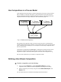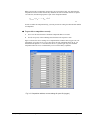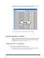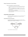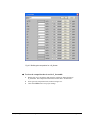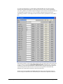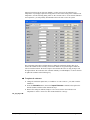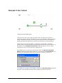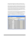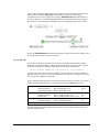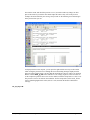
1
IPSEpro Process Simulator
Enginomix Power Plant Library
IPSEpro Process Simulator
Enginomix Power Plant Library
Library Version 1.017
Manual Version 1.017.04
Copyright: Enginomix LLC, 2009
Contents
1. Introduction ............................................................................................... 1-1
The Enginomix Power Plant Library ............................................................... 1-1
About this Manual ........................................................................................... 1-1
Related Documents .......................................................................................... 1-2
Assumptions .................................................................................................... 1-2
Conventions ..................................................................................................... 1-3
Definitions .................................................................................................................... 1-3
Typographical Conventions .......................................................................................... 1-3
Keyboard Conventions ................................................................................................. 1-4
Mouse Techniques ........................................................................................................ 1-4
Installing the EPP Library................................................................................ 1-5
2. Library Overview ..................................................................................... 2-1
Design Considerations ..................................................................................... 2-1
Off-Design Behavior........................................................................................ 2-1
Library Components ........................................................................................ 2-2
3. Physical Properties and Chemical Compositions................................... 3-1
Physical Properties........................................................................................... 3-1
Water and Steam Streams (W_Stream)......................................................................... 3-1
Gas Streams (G_Stream)............................................................................................... 3-3
Gas Compositions in a Process Model ............................................................ 3-4
Defining a Gas Stream Composition ............................................................... 3-4
Using a Composition in a Stream .................................................................... 3-6
Defining a Composition for a Single Stream ................................................................ 3-6
Defining a Composition for a Group of Streams .......................................................... 3-7
Compositions and the System .......................................................................... 3-7
Units that Do Not Change Compositions ...................................................................... 3-7
Mixing Streams ............................................................................................................. 3-8
4. Examples .................................................................................................... 4-1
Terminology..................................................................................................... 4-1
Example 1: Stream........................................................................................... 4-2
Example 2: Simple Steam Cycle ..................................................................... 4-9
Example 3: Steam Cycle with Deaerator ....................................................... 4-17
Design Model ............................................................................................................. 4-17
Off-Design Model ....................................................................................................... 4-18
Example 4: Combustion ................................................................................ 4-24
Example 5: Gas Turbine ................................................................................ 4-32
IPSEpro - Enginomix Power Plant Library
Rev. 1.017.04
Contents-I
Example 6: Heat Recovery Steam Generator ................................................ 4-38
Example 7: Integrating Gas Turbine, Heat Recovery Steam
Generator and Steam Cycle ........................................................................... 4-41
5. Demo Samples ........................................................................................... 5-1
6. To Comment on this Documentation ...................................................... 6-1
Index ............................................................................................................... 7-1
IPSEpro - Enginomix Power Plant Library
Rev. 1.017.04
Contents-II
1. Introduction
The Enginomix Power Plant Library
The Enginomix Power Plant Library for IPSEpro has been designed for modeling a wide range
of thermal systems. The design of this library is based on many years of experience, gained with
the power process modeling package IPSE.
The Enginomix Power Plant Library allows you to design and analyze any power plant,
including:
•
Combined-cycle plants.
•
Cogeneration plants.
•
Conventional fossil-fueld plants.
The library contains models for both design and off-design analysis.
The way that the Enginomix Power Plant Library was designed, using the Model Development
Kit (MDK) of IPSEpro, allowed the creation of extremely powerful component models.
About this Manual
This documentation describes the Enginomix Power Plant Library for IPSEpro, to be used in
PSE projects. It provides information for both new and experienced users of PSE. For a
comprehensive description about PSE, refer to the IPSEpro-PSE User Manual.
If you are a new user, you find in this documentation a series of examples created with the
Enginomix Power Plant Library. These examples explain you how to set up a power plant
model. It also shows how the system reacts on the most frequent input errors.
If you are an experienced user of PSE, you find in this documentation information about some
aspects that are specific to the Enginomix Power Plant Library.
This manual contains six chapters, as described below:
Chapter 1 introduces the Enginomix Power Plant Library and establishes the assumptions and
conventions used in this documentation.
Chapter 2 describes the design considerations and the available components of the Enginomix
Power Plant Library.
Chapter 3 provides information about the physical properties and the chemical compositions
used in the Enginomix Power Plant Library.
IPSEpro - Enginomix Power Plant Library
Rev. 1.017.04
Page 1-1
Chapter 4 shows various examples of process models in PSE, using the Enginomix Power Plant
Library.
Chapter 5 explains how you can use the models available as Demo samples for the Enginomix
Power Plant Library.
Chapter 6 tells you how you can comment on this documentation.
Related Documents
You will find further information in the following documents:
•
Library Reference Documentation. You find a detailed description of the models that are
included in the Enginomix Power Plant Library in the on-line help file. If you prefer a
hardcopy version of the documentation, you can print the rich text file (.rtf) that comes
with the library.
•
IPSEpro-PSE documentation. This document is part of the Process Simulation
Environment (PSE). It provides information about how to use the IPSEpro libraries for
setting up process models and running calculations in IPSEpro.
•
IPSEpro-MDK documentation. This document is part of the Model Development Kit
(MDK). It provides information about creating model libraries for IPSEpro.
•
For questions specific to the operation system, please consult your Microsoft-Windows
documentation.
Assumptions
Throughout this documentation, the following assumptions are made:
•
Windows refers to Microsoft Windows XP, Service Pack 2 or higher versions of that
program. Most information applies also to Windows NT, although there are differences in
the graphical appearance of the systems.
•
You have completely installed Windows on your computer. If you have not yet installed
Windows, please run Windows Setup before installing IPSEpro. Refer to your WindowsDocumentation on how to install Windows.
•
You have completely installed IPSEpro-PSE on your computer. If you have not yet
installed IPSEpro, please run PSE (& MDK) Setup. Refer to your IPSEpro Installation
Guide on how to install IPSEpro.
•
You are familiar with the IPSEpro-PSE Documentation.
•
You are familiar with the handling of standard Windows-programs. You find the required
information in your Windows-Documentation.
•
You are familiar with the handling of a mouse.
IPSEpro - Enginomix Power Plant Library
Rev. 1.017.04
Page 1-2
Conventions
This documentation uses the following definitions and typographic conventions:
Definitions
process scheme, flowsheet: The graphical representation of your project in your PSE project
window is called process scheme, or flowsheet.
model, process model: The mathematical representation of a process scheme is called process
model, or just model.
project: A project is the collection of all available information about a process model. A project
consists of several process files, which PSE manages automatically after a project is opened. All
project files of a project are in the same directory and have the same filename, with different
extensions.
library icon, unit icon: The graphical representation of a component of an IPSEpro library,
available for building a process scheme, is called library icon, unit icon, model icon or just icon.
component model, component: The mathematical representation of an IPSEpro library
component, within a process model, is called component, component model, or just model
(whenever its meaning does not conflict with process model).
object: All elements contained in a project are called objects. Besides component models,
connections and compositions, additional objects, such as data-frames, text- and OLE-objects
can be used in a project.
Typographical Conventions
As far as possible, this documentation uses the same typographical conventions as the Windows
documentation. In particular, the following typographical conventions are used throughout this
documentation:
Style
Meaning
Italic
Indicates a placeholder for information. For example, if
you are asked to type filename, you must type the actual
name of the file instead of the italic printed word.
Bold Italic
Indicates text that must be entered exactly as printed.
It also indicates new terms. The explanation follows
immediately after the term printed bold italic.
ALL UPPERCASE
Directories, filenames
Bold upper-/lower case
Menu elements and names of commands. For example
menu File, command Save
SMALL CAPITALS
Key names - for example CTRL-KEY, DEL-KEY.
[[optional]]
Expressions in double brackets are optional
IPSEpro - Enginomix Power Plant Library
Rev. 1.017.04
Page 1-3
Keyboard Conventions
The key names in this documentation appear in small capital letters. For example, the shift key
appears as SHIFT.
A plus sign (+) between key names means that you must press the keys at the same time. For
example, SHIFT+F1 means you press and hold down SHIFT while you press F1.
A period (,) between key names means that the keys must be pressed sequentially. For example,
means you first press and release ALT, then press and release E, and finally press O.
ALT, E, O
Mouse Techniques
In the description of mouse operations the following expressions are used:
Primary mouse button. Typically the left button of your mouse is the primary button. Since lefthanded users can swap the mouse buttons in Windows, this button is called the primary mouse
button, and not the “left button”.
Secondary mouse button. Typically this is the right button of your mouse. For the same reasons
mentioned above, this button is called the secondary mouse button.
Click. If you are instructed to click on a particular object, you place the cursor on this object,
press the primary mouse button and release it immediately.
Double click. To double click on an object, place the cursor on this object and press the primary
mouse button twice. If the two clicks happen within a certain period, Windows interprets this as
a double click.
Drag. For dragging, you press the primary mouse button and move the mouse while you keep
down the button. When you have finished the operation, release the primary mouse button
again.
IPSEpro - Enginomix Power Plant Library
Rev. 1.017.04
Page 1-4
Installing the EPP Library
You received the Enginomix Power Plant Library as a compressed model library (CML) either
on a CD or by downloading from the Enginomix web site. The library is packed in a file
EPP_Lib.CML. You install any libraries you downloaded or from the CD in the same way.
⇒
To install the EPP Library:
1.
Go to the EXE directory of your IPSEpro installation.
2.
Start the library installer LIBINST.EXE.
3.
Follow the instruction of the SETUP program.
4.
When you are asked to select a model library select EPP_LIB.CML on your distribution
medium.
If you have any problems in accessing the Enginomix Power Plant Library from PSE, check
that the required assumptions are fulfilled and remove any obstacles. If the problem remains,
contact Enginomix Technical Support Services and give a precise description of your
problem.
E-mail: [email protected]
Tel:
[+ 1] (650) 289-0670
IPSEpro - Enginomix Power Plant Library
Rev. 1.017.04
Page 1-5
IPSEpro - Enginomix Power Plant Library
Rev. 1.017.04
Page 1-6
2. Library Overview
This chapter introduces the design considerations of the Enginomix Power Plant Library, and
lists its available components.
Design Considerations
The Enginomix Power Plant Library has been implemented with the aim of enabling users to
model a wide range of thermal power plants. The library models have been carefully designed to
provide a balance among ease-of-use, engineering detail and accuracy and flexibility.
In the course of a project, you will frequently have a varying demand on the component models
that you are using. AT the beginning of your project, you may only have preliminary data
available to use to set up your component models. At this stage, you will most likely prefer to
use some of the simpler component models. When you have more detailed data available, you
can switch to the more detailed engineering models provided for many of the key equipment
components, without having to rebuild your project.
For each library unit of the Enginomix Power Plant Library, a default model is available, which
guarantees fast results in the simulation phase. In order to achieve this, the following aspects
have been taken into account:
•
Minimal data input required by the user.
•
Simple mathematical formulation in order to achieve fast convergence.
In PSE, when you select a library unit to become a new object of your process model, this object
automatically uses its built-in default model.
If required, you can switch to another model for each equipment unit. For example, you may
wish to use the model for off-design calculations, or for some components you may want to use
design models that include more engineering or geometry-based details. You can also base your
off-design models on results obtained with the design model of the process.
Off-Design Behavior
Specialized off-design models are available for key equipment units in the Enginomix Power
Plant Library.
While some of the design component models focus on few data input and on fast convergence,
typically the off-design models emphasize the following aspects:
•
Optimum interaction with the design models.
•
Models are valid on a general basis.
•
Good balance between required input and accuracy.
IPSEpro - Enginomix Power Plant Library
Rev. 1.017.04
Page 2-1
In a PSE project, you can use off-design models of the selected library units to build different
calculation layers (datasets) of the process scheme. Usually, you first define a process model in
the design mode, which feeds data to further off-design process models. In these off-design
process models, you can simulate your process with different part loads.
Refer to the IPSEpro-PSE Documentation, for more details about model refinement,
datasets management, and off-design modeling.
Library Components
This section provides a list of the units of the current library. For more details about each of the
library components, you should refer to the library on-line help file, and to the library
hardcopy documentation. These documents will always provide the most update description
version of your library. This is especially true if your IPSEpro installation includes the model
development kit (MDK), since you can change the libraries yourself with the MDK (and update
the on-line help file or library documentation files).
The hardcopy documentation of a model library contains all the available information about the
included component models. You can read the library hardcopy documentation file, using any
program that supports the rich text format (files with the .rtf extension).
The on-line help file can be accessed directly from PSE. This file contains the same information
of the hardcopy documentation about the library component models.
The following table lists all units that are available in the Enginomix Power Plant Library.
Unit Name
Description
EPP_Data_Stream_Splitter
splitter for data/info streams
EPP_Fuel_Sink
sink for a fuel_stream
EPP_Fuel_Source
source for a fuel_stream
EPP_Fuel_Water_Mixer
mixer for fuel and water to create a fuel_water stream to
feed to further processing equipment
EPP_Fuel_Water_Pump
pump for fuel_water stream (fuel/water mixture)
EPP_GT_Combustor
combustion chamber model with fuel as chemical
composition. Part of a set of special GT icons – not
recommended for general use!
EPP_GT_Compressor
General off-design compressor model. Part of a set of
IPSEpro - Enginomix Power Plant Library
Rev. 1.017.04
Page 2-2
special GT icons – not recommended for general use!
EPP_GT_Cooling_Air_Mixer_1
virtual cooling air mixer - for GT stator. Part of a set of
special GT icons – not recommended for general use!
EPP_GT_Cooling_Air_Mixer_2
virtual mixer for cooling air into gas turbine hot gas flow.
Part of a set of special GT icons – not recommended for
general use!
EPP_GT_Exit_Diffuser
diffusor models for gas turbine exit. Part of a set of
special GT icons – not recommended for general use!
EPP_GT_Expander
turbine expander section model. Part of a set of special
GT icons – not recommended for general use!
EPP_GT_Generator
electric generator. Part of a set of special GT icons – not
recommended for general use!
EPP_G_Bellmouth
bellmouth (gas turbine inlet)
EPP_G_Chiller
gas chiller
EPP_G_Combustor
combustion chamber model with fuel specified by
chemical composition (gaseous fuels)
EPP_G_Inlet_Diffuser
inlet diffuser for gas turbine combustor inlet
EPP_G_Compressor
gas compressor
EPP_G_Compressor_extr
general compressor model with extraction connections
and off-design modeling capability
EPP_G_Expander
gas turbine expander section model
EPP_G_Exit_Diffuser
exit diffuser model for gas turbine exit
EPP_G_Fan
fan for gas streams
EPP_G_Htex
general purpose heat exchanger for gas streams
EPP_G_Monitor
gas monitor icon for calculating and setting gas stream
properties
EPP_G_W_Double_Htex
heat exchanger with gas stream on hot side and two
water/steam streams on two cold side
EPP_G_W_Htex
heat exchanger with gas stream on hot side and
water/steam stream on cold side
EPP_G_W_Injector
injection cooler for injecting water/stream in to gas
stream
EPP_Gearbox
gearbox
IPSEpro - Enginomix Power Plant Library
Rev. 1.017.04
Page 2-3
EPP_Generator
electric generator
EPP_HA_CoolingTower
cooling tower using special humid-air gas streams – to
cool water stream, humidifying and heating gas stream
EPP_HA_Fan
fan for humid air streams
EPP_HA_Inlet
icon to convert general gas stream to special humid-gas
stream
EPP_HA_Outlet
icon to convert special humid gas stream back to general
gas stream
EPP_Monitor_Ambient
display and set ambient conditions from the flowsheet
EPP_Motor
electric motor
EPP_Plant_Summary
calculate and display power plant summary variables
EPP_W_Attemperator
spray attemperator – spray water into steam stream to
control temperature
EPP_W_Bidir_Mixer
mixer for water streams that allows flow in either
direction (negative flow rates permitted)
EPP_W_Bidir_Splitter
splitter for water streams allows flow in either direction
(negative flow rates permitted)
EPP_W_Boiler
pulverized coal boiler
EPP_W_Bushing
steam turbine bushings
EPP_W_Chiller
water chiller
EPP_W_Condenser
water-cooled steam condenser
EPP_W_Condenser_ACC
air-cooled steam condenser
EPP_W_Data_Input
data controller for steam/water streams – using data/info
stream connection
EPP_W_Data_Xmitter
data source from steam/water streams – generates
data/info signals
EPP_W_Drum
drum separator (saturated vapor and saturated liquid exit
streams)
EPP_W_Evaporator
natural circulation evaporator (integrated drum)
IPSEpro - Enginomix Power Plant Library
Rev. 1.017.04
Page 2-4
EPP_W_FlowBalance
Flow balancing icon for steam/water streams –
automatically calculate makeup or overflow flow rates to
balance main inlet and outlet flows
EPP_W_Header
header for water and steam streams (combined mixer and
splitter)
EPP_W_Htex
general purpose heat exchanger, steam/water on both
sides
EPP_W_Labyrinth
labyrinth gland seal model
EPP_W_Mixer
mixer for water streams
EPP_W_Pipe
pipe for steam/water streams
EPP_W_Pump
pump for water streams
EPP_W_SSR
steam seal regulator
EPP_W_ST
detailed steam turbine model for HP and IP sections with
optional single extraction
EPP_W_ST_end
detailed condensing steam turbine model for LP sections
with optional single extraction and exhaust loss
EPP_W_ST_end_3extr
detailed condensing steam turbine model for LP sections
with two or three extractions and exhaust loss
EPP_W_ST_end_5extr
detailed condensing steam turbine model for LP sections
with four or five extractions and exhaust loss
EPP_W_Turbine
steam turbine model with no extractions
EPP_W_Turbine_end
condensing steam turbine model for LP sections with
exhaust loss and no extractions
EPP_W_Valve
steam/water valve model
EPP_W_Valve_Chest
steam valve chest
G_Ambient_Sink
release of a gas stream at ambient pressure
G_Ambient_Source
source for a air stream at ambient conditions
G_Analyzer
gas analyzer gives detailed information on gas
composition
G_Condenser
gas condenser
G_Connector
connector for closed gas-stream loops
IPSEpro - Enginomix Power Plant Library
Rev. 1.017.04
Page 2-5
G_Gas_Turbine
gas turbine, with optional GT correction curves
G_Mixer
mixer for gas streams
G_Pipe
pipe for gas streams
G_Sink
sink for a gas stream
G_Source
source for a gas stream
G_Splitter
splitter for gas streams
G_Stream_to_stream
transition piece to convert from G_Streams to streams
G_Valve
valve for gas streams
W_Boiler
simple steam boiler
W_Connector
connector for closed steam/water loops
W_Cooling_Tower_dry
dry cooling tower
W_Cooling_Tower_wet
wet cooling tower
W_Deaerator
deaerator
W_G_Htex
heat exchanger with steam/water on hot side and gas on
cold side
W_Preheater
preheater (feedwater heater)
W_Preheater2
preheater (feedwater heater) with drain cooler zone
W_Preheater3
preheater (feedwater heater) with both desuperheating
and drain cooler zones
W_Separator
water/steam separator
W_Sink
sink for a water stream
W_Source
source for a water stream
W_Splitter
splitter for water streams
W_Stream_to_stream
transition piece to change from W_Stream to general
stream
W_Xprescription
prescription/calculation of steam quality
IPSEpro - Enginomix Power Plant Library
Rev. 1.017.04
Page 2-6
3. Physical Properties and Chemical Compositions
This chapter explains how physical properties are handled in the Enginomix Power Plant
Library.
The first part of this chapter provides a list of all available chemical components, and the
limitations that apply to each of them.
The second part explains how the physical properties are used in PSE projects. It introduces the
concept of compositions and explains how you deal with compositions in your projects.
Physical Properties
The Enginomix Power Plant Library includes a database of physical properties for water and for
a wide range of chemical components that might be used in the combustion system.
Water and Steam Streams (W_Stream)
For calculating the properties of pure water and steam streams (W_Stream connections in
EPP_Lib), you can choose one of the following formulations:
IAPWS_IF97. The IAPWS Industrial Formulation 1997 for the Thermodynamic
Properties of Water and Steam1.
IFC67. The 1967 IFC Formulations for Industrial Use2.
When you install the Advance Power Plant Library, the IAPWS_IF97 equations are selected.
IAPWS_IF97 is the internationally agreed standard. Therefore it should be used in new projects.
However, in older projects you may still want to use the IFC67 formulations.
Switching Between the Two Formulations
⇒
To change the method that is used for calculating the properties of water and
steam:
1.
1
2
In the Windows Start menu select the command PPSwitch in the IPSEpro group.
Windows displays the following dialog, that reflects the current configuration:
Wagner, W., Kruse, A.: Properties of Water and Steam, Springer-Verlag Berlin Heidelberg New York, 1998
Schmidt, E.: Properties of Water and Steam in SI-Units, Springer-Verlag Heidelberg New York, 1969
IPSEpro - Enginomix Power Plant Library
Rev. 1.017.04
Page 3-1
2.
Select the appropriate method and click on the OK button. The configuration is changed to
reflect your selection.
After you have selected a new method, all calculations will be made with the new method.
If you have more than one copy of EPP_Lib installed on your system, make sure that you
switch the correct version. The PPSwitch command in the Windows Start menu always
switches the most recently installed copy.
When you are using IAPWS_IF97, the following limits for temperatures and pressures apply:
Limits for Water
min
max
Temperature [°C]
0.01
2000.0
0.01 °C <= t <= 800 °C
0.1e-6
1000.0
800 °C <= t <= 2000 °C
0.1e-6
100.0
Pressure [bar]
The IFC formulations are defined for temperatures of up to 800 °C. In the Enginomix Power
Plant Library, this range has been extended to 850 °C, due to numerous requests of IPSEpro
users. Since the range from 800.0 to 850.0 °C is not covered by the IFC formulations, it is your
responsibility to verify if results are accurate enough for your specific purpose. Generally, the
results are still satisfying for this range. The range up to 800.0 °C is not affected by the adopted
extension.
IPSEpro - Enginomix Power Plant Library
Rev. 1.017.04
Page 3-2
Gas Streams (G_Stream)
The physical properties of components in gas streams, using the G_Stream connections in
EPP_Lib, are calculated with polynomials derived from the JANAF Thermochemical Tables3.
All calculations are based on the assumption that the chemical components can be treated as
ideal gases. The extent to which the ideal gas formulations yield acceptable accuracy depends
on your specific application: While an inaccuracy of five percent might be unacceptable for a
pure substance, it will be by far accurate enough if a mixture contains only a few percent of this
substance. In practical usage, calculations for exhaust gas systems are nearly always done using
ideal gas formulations.
The following table lists the chemical components that are available in the physical properties
database. The table also provides the temperature and the pressure range that is permitted by the
system.
Variable
3
Component
Temperature [°C]
Pressure [bar]
min
max
min
max
AR
Argon
-30.0
5726.85
0.1e-6
20.0
C2H6
Ethane
-30.0
5726.85
0.1e-6
35.0
C3H8
Propane
-25.0
5726.85
0.1e-6
35.0
CH4
Methane
-30.0
5726.85
0.1e-6
35.0
CO
Carbon monoxide
-30.0
5726.85
0.1e-6
100.0
CO2
Carbon dioxide
-30.0
5726.85
0.1e-6
35.0
H2
Hydrogen
-30.0
5726.85
0.1e-6
35.0
H2O
Steam (as ideal gas)
-30.0
5726.85
0.1e-6
30.0
H2S
Hydrogen sulfide
-20.0
5726.85
0.1e-6
100.0
N2
Nitrogen
-30.0
5726.85
0.1e-6
35.0
O2
Oxygen
-30.0
5726.85
0.1e-6
35.0
SO2
Sulfur dioxide
0.0
5726.85
0.1e-6
10.0
JANAF Joint Army Navy Air Force Thermochemical Tables
IPSEpro - Enginomix Power Plant Library
Rev. 1.017.04
Page 3-3
Gas Compositions in a Process Model
In the Enginomix Power Plant Library, chemical compositions are not part of the gas streams
that are available to connect the units using G_Stream connections. The streams reference
separate compositions which are available in the library. This way, all streams with the same
composition reference one single composition. This is illustrated by figure 3.1.
G_Stream
G_STREAM001
G_Stream
G_STREAM002
G_Stream
G_STREAM003
composition
GAS_COMP
Fig. 3.1: Streams and compositions
The advantage of this approach is that a stream can represent any flow of a medium that is
available in the physical properties database. It does not matter if the stream represents the flow
of air, combustion gases or natural gas. As a consequence, also the library components can be
used on a general basis.
Compositions are implemented as global objects. Compositions are defined in terms of their
mass fractions. Each mass fraction is represented by a variable. If the variable CO2 of a
composition is equal 0.5, this means that 50 percent of the mass of the composition is CO2.
The next section explains how you can define a composition in PSE.
Defining a Gas Stream Composition
⇒
To define a composition you do the following:
1.
Choose from menu Objects the command New Global Object to create the
composition. Once you have created the composition, you can open it for editing.
2.
Edit the composition just created by using the command Edit Global Object of the
Objects menu.
See more details about these commands in the IPSEpro-PSE Documentation.
IPSEpro - Enginomix Power Plant Library
Rev. 1.017.04
Page 3-4
When you prescribe a composition, always take care to prescribe it fully. You must enter the
composition in terms of mass fractions. By definition, the sum of all mass fractions is equal to
1.0. Therefore, the following equation is part of the composition model:
µWATER + µ AR + K + µ So = 1.0
2
3.1
In order to define the composition fully, you must provide one setting less than the total number
of components.
⇒
To prescribe a composition correctly:
1.
Set to zero all mass fractions of chemical components that are not used.
2.
Set all, except one, of the remaining mass fractions to the respective value.
Figure 3.2 shows the correct settings for a composition that contains 100% oxygen (O2). All
components, except O2, are set to zero. Since O2 is the only component that is not set, it is
calculated from equation 3.1. Note that since this is a G_Stream (gas only), the WATER
component cannot be set (it is automatically set to 0.0 in the library equations)
Fig. 3.2: Composition window, correct settings for pure O2 (oxygen)
IPSEpro - Enginomix Power Plant Library
Rev. 1.017.04
Page 3-5
Figure 3.3 shows a frequent mistake that is made when defining the compositions. The oxygen
(O2) component is set to 1.0, but the remaining components are undefined.
Fig. 3.3: Composition window, wrong settings for pure O2 (oxygen)
Using a Composition in a Stream
In PSE, you can define a composition for each gas stream inyour process. However, instead of
defining the used composition for each gas stream separately, you can also define or set one
composition object for a group of gas streams. In this case, all streams selected will use the
same composition (the composition does not change).
Defining a Composition for a Single Stream
⇒
To define the composition that is used in a stream:
1.
Double click on the stream. PSE opens the window for editing the data of that stream.
2.
Select in the composition field the composition that you want to use.
IPSEpro - Enginomix Power Plant Library
Rev. 1.017.04
Page 3-6
Defining a Composition for a Group of Streams
⇒
To set the composition for a group of selected streams:
1.
Select those streams for which you want to set the composition. It does not matter if you
select other objects. If they do not contain references to compositions, they are simply
ignored.
2.
Select the command Set References from the Objects menu. PSE opens a window
where you can select the type of reference that you want to set and the composition that
you want to reference.
3.
From the list of references select composition. Once you have made this selection, PSE
displays all available objects of type composition.
4.
Select the composition that you want to use in the selected streams, and click on the OK
button to accept your choice.
Compositions and the System
PSE requires that you define a correct mathematical system. If you use compositions incorrectly,
you may create a system that is mathematically incorrect. The consequences are usually
convergence problems.
Units that Do Not Change Compositions
The majority of the units in the Enginomix Power Plant Library do not change the chemical
composition in a stream. They simply use the composition of the attached stream to calculate the
required physical properties. See figure 3.4 for an illustration.
Unit
Stream
Stream
Composition
Fig. 3.4: Units that do not change compositions
IPSEpro - Enginomix Power Plant Library
Rev. 1.017.04
Page 3-7
Streams that are attached to a unit that does not change the composition must always
reference the same composition!
Mixing Streams
If you mix two gas streams of different given compositions and of different given mass flows,
the product is a third composition. The mixer model of the Enginomix Power Plant Library
takes into account the composition from the input streams and their respective mass flows, to
calculate the mixed composition. Therefore, you must not prescribe the composition of the
product stream. If you do so, you will create an over-determined system that will usually not
converge.
However, if the same composition is used by the streams that are connected to the mixer, the
mixer model takes into account this situation and delivers the same composition as a product.
Hence, it is also possible to use mixers together with one single composition used by all streams.
IPSEpro - Enginomix Power Plant Library
Rev. 1.017.04
Page 3-8
4. Examples
In this chapter you find step-by-step instructions for setting up several simple process schemes,
using the Enginomix Power Plant Library. These examples serve as a starting point for bigger
projects.
The examples included here are also available in files, together with the library, in order to
make it easier for you to trace mistakes. In the files, not only the final results have been stored,
also results of intermediate steps. This allows you to compare your own results with the
examples’ results.
The files containing the examples are stored in the DATA sub-directory of your EPP_Lib
installation.
Even if you dislike reading manuals, you are strongly encouraged to read through this
section, since it provides you with the minimum of information required to use PSE and
the Enginomix Power Plant Library!
Terminology
Whenever a file is stored, in the description of the examples of this chapter, you find the
indication in the text in the following way:
Ex_aa_bb.pro ⇐
The file name is composed of an Ex_ prefix, two digits identifying the example number, and
two digits identifying the step number, separated by an underscore “_”.
If during your training phase with PSE and the Enginomix Power Plant Library, you become
stuck with a problem, you should use these files for comparisons with your project.
IPSEpro - Enginomix Power Plant Library
Rev. 1.017.04
Page 4-1
Example 1: Stream
In this example, you will create a source and a sink that are connected by a gas stream. You will
learn how you define a chemical composition. You will also see how PSE reacts on incorrect
input. After you have created a new, empty project, draw the scheme as shown in figure 4.1:
Fig. 4.1: Gas Stream, flowsheet
⇒
To draw the scheme shown in figure 4.1, do the following:
1.
Click on the G_Source icon in the icon palette. When you move the cursor over the PSE
workspace to your project window, it takes the shape of the icon selected.
2.
Click at the position where you want to place the source icon.
3.
Place a G_Sink icon in your project window, in the same way. Make sure that the sink icon
remains selected.
4.
Press CTRL-R to rotate the sink icon counter clockwise by 90°.
5.
Click on the open box that marks the connection terminal at the tip of the arrow-shaped
representing the gas source. By doing this, you start the connection drawing mode.
6.
Start drawing your connection. Click wherever you want the connection to make a corner
(note that PSE automatically shifts the last corner you make before connecting to another
terminal so that the last corner remains at a right angle).
7.
Click on the box that marks the connection terminal of the sink. PSE terminates the
connection drawing mode, and attaches the connection to the sink.
PSE automatically creates a name for each of the objects. To display the names, choose the
command Object Names from the menu View.
IPSEpro - Enginomix Power Plant Library
Rev. 1.017.04
Page 4-2
By drawing the process scheme you have already set up the major part of the model. What is
still missing is specifications for the stream properties and icon/equipment data. If you start the
simulation now, you will receive the following error message:
Fig. 4.2: Error message for undefined composition object
After you have acknowledged the message by clicking on the OK button, PSE opens the data
window of G_Stream001. (If you have not tried to run the calculation, you can open the data
window of G_Stream001, by double-clicking on the connection that you have drawn.) However,
since you have not yet defined any compositions, you must close this data dialog window to
create the composition object first. You close the dialog window by clicking on its OK button.
Ex_01_01.pro ⇐
⇒
To create a gas composition object:
1.
From menu Objects select the command New Global Object. PSE opens the window
shown in figure 4.3.
2.
Select G_Composition as the type of the global object, and enter gas in the name field.
Click on the OK button to create the new composition.
Fig. 4.3: Dialog for creating new global objects
Ex_01_02.pro ⇐
IPSEpro - Enginomix Power Plant Library
Rev. 1.017.04
Page 4-3
Fig. 4.4: Choosing the composition for editing
You can now define the new composition object GAS, by editing it in the following way:
⇒
To edit the new composition:
1.
From the Objects menu, select the Edit Global Object command. PSE opens the
window shown in figure 4.4.
2.
Select the entry GAS(G_Composition) and click on the Edit >> button. PSE opens the
data window of the composition, as shown in figure 4.5.
3.
Set the mass fraction values for all of the species except N2 to zero. This defines your gas
composition as pure nitrogen (refer to your IPSEpro-PSE Manual for more details about
setting global parameters).
4.
Close the composition window by clicking on the OK button to accept your settings.
5.
Close the Edit Global Object window by clicking on the Close button.
Note that an equation is included in the G_Stream composition object calculations
equating the sum of the mass fractions to 1.0, so when we set all the mass fractions to
0.0 except for N2, PSE automatically calculates the N2 mass fraction to be 1.0.
Now that you have defined a composition, you can also use this composition in G_Stream001.
IPSEpro - Enginomix Power Plant Library
Rev. 1.017.04
Page 4-4
Fig. 4.5: Defining the composition for a G_Stream
⇒
To select the composition that is used in G_Stream001:
1.
Double click on G_Stream001. PSE opens the window for editing the data of
G_Stream001. The composition field of this window shows “No Selection”.
2.
Select gas in the composition field, as shown in figure 4.6.
3.
Click on the OK button to accept your settings.
IPSEpro - Enginomix Power Plant Library
Rev. 1.017.04
Page 4-5
Fig. 4.6: G_Stream data window
Ex_01_03.pro ⇐
Try running the calculation again. Select from the Calculation menu the command Run
Simulation. PSE will run through the calculation phase, and will return with the following
message:
Click on the Yes button. PSE opens the protocol where you find more details about the error
that has occurred.
Scroll the protocol screen to read the following error message line:
%Error: Problem undefined: 17 equations, 20 variables
You have to prescribe three (20-17=3) more variables in order to make your system well
defined. You are free to choose the variables that you prescribe, as long as the prescriptions are
not mutually exclusive.
IPSEpro - Enginomix Power Plant Library
Rev. 1.017.04
Page 4-6
If the difference between equations and variables is more than three, you may have set
the composition incorrectly. Check the settings of your composition, before you
prescribe the missing variables.
Switch back to the project window or close the error protocol. PSE now displays a cross
attached to the connection that shows the results obtained for the variables of the connection. A
color scheme defines the status of the values displayed as follows:
Black
The value is a converged variable or a parameter.
Red
The variable did not converge.
Blue
The variable has not been calculated.
You can insert a reference cross to make it easier to identify the results variables automatically
displayed in the data crosses attached to the streams after you run the simulation.
⇒
To insert a reference cross:
1.
From the Objects menu, select the command Add Reference Cross. PSE opens a
window where it displays a list of all available connection models.
2.
From the list of available connection models, choose G_Stream.
3.
Click on the OK button. PSE inserts the reference cross in the lower left corner of the
workspace. You can drag it to any other position of your project window.
Since the model is undefined, you have to set more variables. Choose, for example, the
following input settings:
G_Source
G_Source001
p
t
mass
1.0
500.0
1.0
bar
°C
kg/s
Ex_01_04.pro ⇐
It is equally valid to set the mass flow at the sink, instead of at the source. You can do this with
the following inputs settings:
G_Source
G_Source001
G_Sink
G_Sink001
p
t
mass
1.0
500.0
1.0
bar
°C
kg/s
However, if you try to set the mass flow at both the sink and source, PSE will generate an error
called a structural singularity. To see this error in your example model, set the variable mass at
the sink to 1.0 and remove the setting for the temperature.
Ex_01_05.pro ⇐
IPSEpro - Enginomix Power Plant Library
Rev. 1.017.04
Page 4-7
If you run the example again, PSE now writes the following error message to the protocol:
%Error:
System structurally singular, 1 equations depending
Variable G_Stream.s can not be calculated
G_Source G_Source001 equation f_mass is redundant.
Redundant equation contains the following variables:
G_Stream001.mass
IPSEpro - Enginomix Power Plant Library
Rev. 1.017.04
Page 4-8
Example 2: Simple Steam Cycle
This example explains the steps that you must take to set up a model for the simple steam cycle
shown in figure 4.7. In this example, you will learn about specific aspects of closed cycles and
details about some of the key steam cycle equipment models.
Note that when you use IPSEpro in your work, you will rarely start a new project model
completely from scratch. Almost always, you will modify existing projects you created
earlier or from the sample library to match your new requirements. With this approach,
you will save a considerable amount of time, particularly for larger, more complex
projects.
Fig. 4.7: Simple steam cycle, flowsheet
Figure 4.7 shows the steam cycle project that you will create in this example. Note that this
steam cycle is in a closed loop. This requires some additional considerations. During the
solution of the model equations the mass balances for each of the units is calculated, among
other things. With a closed cycle, one of the mass balance equations is redundant, since it is
automatically satisfied. Figure 4.8 illustrates this situation for a pair of pipes connected on both
ends (note that in this figure, the two mass balance equations in the two pipe icon models are
essentially identical).
IPSEpro - Enginomix Power Plant Library
Rev. 1.017.04
Page 4-9
Fig. 4.8: Mass balances for a closed cycle
In order to remove the redundant mass balance from a closed cycle model, you must include a
connection element somewhere in the closed loop, as shown in the sample model in figure 4.8.
Now, construct the model diagram as shown in Figure 4.8. You will need to insert the following
icons into your model diagram:
Water/Steam boiler
Steam turbine
Steam condenser
Water pump
Water/Steam connector icon
Electrical generator
Water/Steam source
Water/Steam sink
W_Boiler
EPP_W_ST
EPP_W_Condenser
EPP_W_Pump
W_Connector
EPP_Generator
W_Source
W_Sink
As you scroll through the icon palette in PSE, you will see that many of the component models
in EPP_Lib have more than one icon representation. For example, the condenser component
(EPP_W_Condenser) has two different icons, each a mirror image of the other, as shown here:
Multiple graphical icons are included for some components in EPP_Lib simply to help you
arrange your model diagram. The stream connections, model equations and variables are always
identical for all of the icon representations for a given component. You can choose whichever
icon looks best, depending on how you want to arrange the graphics for your model diagram. In
this example, we would choose the EPP_W_Condenser icon on the left if we want our model
diagram to look like the sample diagram in Figure 4.7.
For some of the component models you need to include in this simple example, you may find
several different components in the icon palette which might be the one you’re looking for. For
example, if you need to add a steam turbine to your model, until you are more familiar with all
of the component models available in EPP_Lib, you may puzzle over which steam turbine
component you should choose. In this tutorial example, we have told you which steam turbine
component to include (EPP_W_ST), but you will need to familiarize yourself with the available
component models to understand which one to include in other projects you want to build,
depending on what your requirements are.
IPSEpro - Enginomix Power Plant Library
Rev. 1.017.04
Page 4-10
All of the available component models were listed in the table in Chapter 2, Library Overview.
Here are the steam turbine component models listed in that table, along with their respective
icons displayed in the icon palette in PSE:
EPP_W_ST
detailed steam turbine model for
HP and IP sections with optional
single extraction
EPP_W_ST_end
detailed condensing steam turbine
model for LP sections with
optional single extraction and
exhaust loss
EPP_W_ST_end_3extr
detailed condensing steam turbine
model for LP sections with two or
three extractions and exhaust loss
EPP_W_ST_end_5extr
detailed condensing steam turbine
model for LP sections with four or
five extractions and exhaust loss
EPP_W_Turbine
simplified steam turbine model
with no extractions
EPP_W_Turbine_end
detailed condensing steam turbine
model for LP sections with exhaust
loss and no extractions
When selecting the icon you want to use for one of the steam turbine components, you will also
need to familiarize yourself with the connecting terminal (stream) locations on those icons,
because otherwise you may not select the best icon representation for the model you are trying
to build. For example, there are two icon representations for many of the steam turbine
components in EPP_Lib, as shown in the above table. The reason for this is that at the back end
of those steam turbine components, there are two different kinds of exit streams: one is the
primary exit steam stream, which must be connected in any model where you are using that
component model. The other exit stream is for an extraction or leakage stream at the exit of that
steam turbine, and that connection is optional. As displayed in the icon palette, the primary exit
steam connection is on the top of the icon, and the exit extraction/leakage port is at the bottom.
Therefore, if you want the primary steam exit port for your selected steam turbine component to
be on the bottom of the icon when it’s placed on your diagram (as in Figure 4.7), you will need
to select one of the icons and rotate it when you place it in your model diagram. To make your
model diagram to look like that shown in Figure 4.7, select the EPP_W_ST icon on the right in
the icon palette, and rotate it so the primary steam exit connection is on the bottom.
IPSEpro - Enginomix Power Plant Library
Rev. 1.017.04
Page 4-11
To learn about the different connections used for a given EPP_Lib component and the various
icon representations available (and how the connection terminals are oriented), you should
review the on-line help file for the library. For example, if you open the on-line help file for
EPP_Lib and click on the link for the EPP_W_ST component (under “Available units”), the
following graphic is displayed, which can help you choose which icon representation will work
best in your model:
These are the two icon representations included for the EPP_W_ST component model
(displayed side-by-side on the icon palette in PSE). From this graphic, we can see that the
primary steam exit port (“drain”) is at the top of each icon, and the exit extraction port
(“exit_extr”) as at the bottom. If we rotate the bottom of the two icon representations shown
above, the icon will be oriented to match that shown in Figure 4.7, so that is the icon
representation we want in this example. In the icon graphics displayed in the on-line help file,
the labeling of the connecting terminals on each icon also helps to illustrate which connections
are required or optional, and whether or not there are multiple locations for that connection. If a
connection is optional, you can use that component in your project without connecting a stream
to that connection: if a connection is required, you must connect a stream to that connection in
order to use that component model. Connections which are optional are displayed in square
brackets (such as “[exit_extr]” above). Connections which are required are displayed without
brackets (such as “drain” above). Some connections have more than one location available on
the icon (but you can only connect one of them at a time). If a connection has more than one
location, it is displayed in italics (such as the “feed” connection above). If a connection has only
one possible location, it is not displayed in italics (such as “drain” above).
IPSEpro - Enginomix Power Plant Library
Rev. 1.017.04
Page 4-12
When you draw a process model, PSE creates a unique name for each of the objects that you
add to the model (you can change the name at any time if you want). Once you have placed all
of the icons on your diagram, start drawing the connections at the outlet connection for the
connector icon, and proceed clock-wise around the model. PSE will choose the connection
names as shown in figure 4.9. To display the names, choose the command Object Names from
the View menu (note that the icons in the diagram in Fig 4.9 have been moved apart
horizontally in order to display the object names more clearly).
Using this connection element in the steam cycle of figure 4.7, you obtain the model shown in
figure 4.9:
Figure 4.9: Model for a simple steam cycle
Note that since there are no gas streams in this model, you do not have to create any G_Stream
composition objects. In EPP_Lib, pure steam/water streams are of type W_Stream, and the
composition is automatically set to be pure WATER (which can be liquid or gas).
EX_02_01.pro⇐
⇐
If you start the simulation now, you receive the following error message:
PSE has detected that you did not provide data for a parameter. Parameters are numerical values
that always must be defined. Therefore, it is possible to check which parameters have not been
defined. Acknowledge the message by clicking on the OK button. PSE opens the data window
for the respective unit, whose parameter is missing.
IPSEpro - Enginomix Power Plant Library
Rev. 1.017.04
Page 4-13
You have two options to provide the missing parameters:
⇒
•
Enter the parameters manually, by editing the unit data window.
•
Use values from the default value database.
To load default values from the default value database:
1.
From the Objects menu, select the command Load Default Values. PSE opens a
window where you can select if you want to overwrite existing values.
2.
If you have an object selected, PSE offers you to choose to load default values just for the
selected object or for all objects of the project. Make the appropriate settings.
3.
Click on the OK button to load the default values.
EX_02_02.pro⇐
⇐
By definition, it is impossible for PSE to load settings for variables, since the settings depend on
the system configuration and on your specific requirements. Default values for variables are
loaded as estimates and not as settings. Therefore, some additional settings are required. If you
start the simulation now, you receive the following error message:
Select YES to open a window displaying the protocol. The error message from the system is:
%Error: Problem undefined, 90 equations,101 variables
To solve the system successfully you have to set 11 additional variables. You have the
flexibility to choose the variables that are most appropriate for your particular problem. The
selection of these variables requires a certain level of experience. PSE cannot make any
decisions for you about these variables, since the selection depends on your objective.
IPSEpro - Enginomix Power Plant Library
Rev. 1.017.04
Page 4-14
For this example, set the following input variables:
⇒
Steam turbine inlet
W_Stream001
Steam turbine exit
Cooling water inlet
W_Stream002
W_Source001
Steam turbine
Generator
EPP_W_ST001
EPP_Generator001
Condenser
EPP_W_Condenser001
p
t
p
p
t
eta_s
speed
power
eta_el
eta_m
dt_out
40.0
500.0
0.05
1.0
20.0
0.9
3600
2000
0.985
1.0
2.0
bar
°C
bar
bar
°C
---RPM
kW
------°C
To enter the variable values:
1.
Double-click on the respective object. This opens the object data window.
2.
Click on the set button of the variable.
3.
Enter the value in the data field. Note that for some of the variables, you do not need to
type in a value since values may have already been loaded in as estimates from the default
value database.
EX_02_03.pro⇐
⇐
Assume that you are interested in the thermal efficiency of the process. The definition that you
are using is the following:
η=
PGenerator
QBoiler
You can add a data frame that calculates the efficiency according to the equation above.
⇒
To calculate the thermal efficiency:
1.
Select from the Objects menu the command New Data Frame.
2.
Choose that the data frame has 3 columns and one row.
3.
Click in the workspace of your project window, to place the data frame.
4.
The data frame has three cells. Select the first cell and type Efficiency.
5.
Select the second cell.
6.
Type “=”. Then click on the EPP_Generator icon. PSE displays a list with all variables of
the generator.
7. Select power from the list. PSE inserts the string EPP_Generator001.power in the cell.
8. Type the division operator “ / ”.
9. Click on the W_Boiler icon and select heat_input from the list of variables. PSE inserts the
string W_Boiler001.heat_input in the cell.
10. Type the multiplier operator “ * “ followed by 100.0 to convert the fraction to a percent.
11. Select the third cell and type “[ % ]“ to show that the calculated value is a percentage.
IPSEpro - Enginomix Power Plant Library
Rev. 1.017.04
Page 4-15
12. Click on an unused area of the workspace. As soon as the data frame cell is deselected, it
evaluates the equation entered and displays the result.
EX_02_04.pro⇐
⇐
You can now try to prescribe different variables. You can, for example, prescribe the heat input
to the cycle instead of the electrical power output. Do this by prescribing the variable
heat_input for the boiler, instead of power for the generator.
EX_02_05.pro⇐
⇐
IPSEpro - Enginomix Power Plant Library
Rev. 1.017.04
Page 4-16
Example 3: Steam Cycle with Deaerator
In this section, the simple steam cycle model we created previously is extended by adding a
deaerator, as shown in figure 4.10. This example also shows how you create a part-load model
for the extended process scheme.
Figure 4.10: Steam cycle
Design Model
Most of the steam turbine components in the Enginomix Power Plant Library, including the
EPP_W_ST component, contain one or more steam extraction ports. We could have used that
extraction port to connect to our deaerator, but we also can model an extraction by using two
separate steam turbine icons and placing a splitter between them, as shown in Fig 4.10. Using
this approach, you can model any number of extraction streams.
Frequently it is not necessary to develop a model from scratch. It is usually more efficient to
modify existing models based on your current requirements. To illustrate this, start with the
model from Example 2 as the starting point for our new model. Before you start modifying the
model, save the project under a new name, to avoid losing your original model.
First, add the additional icons needed. These include a second steam turbine (EPP_W_ST), a
second pump (EPP_W_Pump), a deaerator (W_Deaerator) and a splitter (W_Splitter). When
you select the steam turbine icon, remember the orientation of the exit ports on that icon from
Example 2: you want to choose the appropriate icon and rotate it so that primary steam exit
connection (“drain”) is at the bottom of the icon. If you place the second turbine icon to use it as
the low-pressure turbine, you will need to disconnect the drain stream connecting the first
turbine to the condenser so that you can instead connect it to the outlet of the new, second
turbine (so this connection will now go from the second turbine to the condenser).
IPSEpro - Enginomix Power Plant Library
Rev. 1.017.04
Page 4-17
⇒
To disconnect a connection from a unit:
1. Type CTRL-F or select the command Free Connection of the Objects menu. The cursor
changes into a scissors symbol.
2. Click on the terminal where the drain stream is attached to the first turbine. By doing so, you
release the connection from that point.
3. By double-clicking on an unused area of the workspace, you create a free-end for this
connection. The free end of a connection is marked by a circle.
EX_03_01.pro⇐
⇐
Now you can carry on setting up the new scheme. Click on the free end of the connection you
just freed (clicking on the circle marking its end) and you are again in the drawing mode of the
connection. Connect that stream to the exit of the second turbine, and then continue drawing all
of the connections as shown in figure 4.10.
You must now enter the parameters for the new units. You can load the default values for the
new icons using the Load Default Values command from the Objects menu.
EX_03_02.pro⇐
⇐
Next, you must set sufficient variables to define the model. Remember to set the pressure of the
bleed stream (either at the exit of the first turbine section, or the inlet of the second turbine
section).
EX_03_03.pro⇐
⇐
Off-Design Model
The major difference between design and off-design or part-load calculations is that you need to
use more detailed unit models for the latter. While it is possible to use the detailed models for
calculating the off-design independently from a design calculation, it is more efficient to base
off-design calculations on the design case:
•
Design cases typically require fewer input data. Results from the design case are often used
as inputs to the off-design cases.
•
A design case typically does not need initial estimates, but off-design cases often do. The
results of the design calculation can be usually be used as good initial estimates for the offdesign cases.
For these reasons, IPSEpro off-design calculations should always be based on a design
simulation. You use PSE’s concept of datasets to establish the relationship between design and
off-design process models. Refer to the IPSEpro-PSE documentation for more details about
managing datasets.
IPSEpro - Enginomix Power Plant Library
Rev. 1.017.04
Page 4-18
Figure 4.11: Dataset manager
The recommended procedure is the following:
1. Run a design simulation first in order to make the design results available.
2. Create an additional dataset in your project.
3. Select the appropriate off-design model for each component of the new dataset, and modify
the settings accordingly.
4. Update the dataset with the data from the design case.
5. Run the simulation for the off-design dataset.
6. PSE provides an efficient mechanism to maintain consistency between design and off-design
cases. You can create additional datasets that store the off-design model. If the design
dataset is modified, you can easily update the off-design dataset to reflect the changes in the
design model.
⇒
To create an additional data set in a PSE project:
1. From the Project menu, choose the command Edit Datasets. PSE opens the window
shown in figure 4.11.
2. Click on the New button and enter a dataset name to create a new dataset (use off-design as
the name of your second dataset for this example). PSE automatically makes the new dataset
active in your project.
3. Click on the Close button. The active project window now displays the new data set.
If there is more than one dataset in your project, it is frequently necessary to switch between
these datasets.
IPSEpro - Enginomix Power Plant Library
Rev. 1.017.04
Page 4-19
⇒
To switch from a dataset to another in a PSE:
1. From the Project menu, choose the Edit Datasets command. PSE opens the Dataset
Manager window.
2. Select the dataset that you want to activate and click on the Activate Dataset button of this
window.
3. Click on the Close button. The active project window displays now the selected dataset.
Proceeding on the construction of the new process model, you have to change the component
settings for the off-design model, in the off-design dataset.
⇒
To change the model that is used for the condenser:
1. Double click on the condenser icon in the worksheet. PSE opens the dialog for editing the
condenser’s data.
2. In the field Model choose the model W_Condenser_pl. PSE opens a window with additional
items displayed for the W_Condenser_pl model.
3. Click on the OK button to accept the modifications. Make sure that the condenser object is
still selected.
4. From the Objects menu, choose the command Load Default Values. PSE opens a dialog
where you choose to load the default values for the selected object.
5. From the Project menu, choose the command Update dataset.
If you open the data window of the condenser again, it will display the data as shown in figure
4.12.
IPSEpro - Enginomix Power Plant Library
Rev. 1.017.04
Page 4-20
Figure 4.12: Data window for the off-design model of the condenser
In the same way done for the condenser, change the data for the remaining models of the offdesign dataset. Change the model selection for the two steam turbine components to
EPP_W_ST_pl, and the boiler model selection to EPP_W_Boiler_pl. Remember to load the
default values and update the dataset after changing any of the icon models to the part-load
methods. See the sample dialog below for typical part-load settings for the EPP_W_ST steam
turbine component.
Do not forget to remove the respective settings in the modified objects. For example
you will no longer be able to set the pressure of the extraction stream. It is a frequent
mistake to forget to remove some settings when switching to off-design models. If you
run the calculation without removing the setting, the system will be over-determined!
EX_03_04.pro⇐
⇐
IPSEpro - Enginomix Power Plant Library
Rev. 1.017.04
Page 4-21
Typical part-load settings for the EPP_W_ST steam turbine component:
Use similar settings for both sections of the steam turbine in your sample model.
IPSEpro - Enginomix Power Plant Library
Rev. 1.017.04
Page 4-22
Frequently, it is useful to create more than one dataset. The datasets can then be organized
hierarchically. Figure 4.13 shows a typical dataset hierarchy.
Figure 4.13: Data set hierarchy
In this example, the first dataset was renamed from “Default” to “Design” to clarify the
relationship among the datasets. You can rename a dataset by choosing the Edit>> command
from the Dataset Manager dialog.
EX_03_05.pro⇐
⇐
IPSEpro - Enginomix Power Plant Library
Rev. 1.017.04
Page 4-23
Example 4: Combustion
In this section you will use the combustion chamber model to calculate the gas/air ratio needed
to achieve a certain exhaust gas temperature, given the inlet conditions and composition for a
fuel gas.
In the EPP_Lib you find several different icon models for combustion chambers. Usually this
applies to liquid and solid fuels. The model G_Combustor is the icon to use if the fuel is
described by its chemical composition, as is the case for gaseous fuels.
First, build the model so it looks like the one shown in Fig. 4.14. This model uses the icons for a
gas source (G_Source), ambient source (G_Ambient_Source), gas monitor (EPP_G_Monitor),
combustor (EPP_G_Combustor) and gas sink (G_Sink). Place these icons on the diagram and
connect them together with gas stream connections (G_Stream).
Figure 4.14: Combustion chamber
EX_04_01.pro ⇐
The next step is to define the required global composition objects, used to store the gas
composition data for each gas stream or set of streams (wherever the gas composition varies due
to mixing or chemical reaction). In this example, you need to create three G_Composition
global objects (using the Objects/New Global Object command), which we will call AIR,
FUEL and EXHAUST_GAS.
After creating the G_Composition objects for the gas streams in our model, we must set the
references for each of the gas streams to link them to the appropriate G_Composition object.
You can do this directly by clicking on each gas stream to bring up the G_Stream data entry
dialog, then selecting the appropriate Composition object for each of the streams.
IPSEpro - Enginomix Power Plant Library
Rev. 1.017.04
Page 4-24
Note that in this model, two of the gas streams should be linked to the same G_composition
object. The two gas streams connected to the G_Monitor icon should both be linked to the
FUEL object, since the G_Monitor icon does not change the composition of the gas stream
passing through it. You can set the references for the two fuel gas streams at the same time by
selecting both streams at once (select one gas stream, then hold down the Shift key and select
the second gas stream), then using the Objects/Set References command to set both
references at once. If you do so, you will see the Set References dialog:
When this dialog appears, select Composition (G_Composition) in the left-side pane (in this
example, that is the only possible selection), and the available G_Composition objects defined
in this project will appear in the right-side pane. Select the FUEL object to set the references for
both fuel streams to that G_Composition object.
After setting the references for all of your gas streams, you can check the selections you have
made by choosing the View/References command option. When you turn this view option on,
your model diagram will show the references you have selected:
Select the View/References command option again to toggle the reference displays off.
Before proceeding further, this is a good time to load default values. Choose the Objects/Load
Default Values command to load defaults and estimated values for the icons and streams.
EX_04_02.pro ⇐
IPSEpro - Enginomix Power Plant Library
Rev. 1.017.04
Page 4-25
The next step is to enter inputs for the stream properties, icon settings and gas compositions that
need to be input by the user for this model. We can start by setting the desired composition of
the air stream that is going into the combustor icon. Use the Objects/Edit Global Object
command and select the AIR object to bring up the dialog for editing the air composition.
Remember that when setting gas compositions, we must leave one composition unspecified,
since the model includes an equation to set the sum of the mass fractions to 1.0. Therefore, if we
want our air composition to be 24% O2 and 76% N2, we could enter the air composition data as
shown here:
Note that we have estimated the desired N2 mass fraction as 0.76, set the O2 mass fraction to
0.24, and set all of the other mass fractions to 0. We also changed the estimate for WATER to 0,
although since this is a G_Composition stream, the model calculations will automatically force
the WATER mass fraction to 0.
IPSEpro - Enginomix Power Plant Library
Rev. 1.017.04
Page 4-26
To set the fuel composition, we could similarly edit the FUEL object to set the fuel mass
fractions. But instead of doing that, we can set the fuel mole fractions in the G_Monitor001
icon. The G_Monitor icon includes equations linking the mole fractions to the mass fractions, so
by setting mole fractions in this icon, we are essentially setting the mass fractions in the
connecting gas streams. Set the inputs for the fuel stream in the G_Monitor001 icon as shown
here:
Note that the estimates values in this dialog (and the other icons and streams in the model) were
set for us when we selected the Objects/Set Default Values command earlier. In the above
example, by setting the mole fractions for C2H6 and C3H8, setting the other mole fractions to
0.0, and leaving the CH4 mole fraction estimated, the icon equations will automatically
determine the required mole fractions for CH4 (0.90 in this case).
We don’t need to set anything for the GAS composition object. The composition of the gas
stream exiting the combustor will be determined by the stoichiometric equations in that icon.
IPSEpro - Enginomix Power Plant Library
Rev. 1.017.04
Page 4-27
For the other required icon and stream inputs, use the following settings (note that depending on
the order you added the icons and streams to your model diagram, you may have slightly
different object names than those shown here):
Air
Fuel
Combustor
mass flow
pressure
temperature
pressure
temperature
air pressure drop
combustion
efficiency
radiation loss
air-fuel ratio
G_Source001.mass
G_Source001.p
G_Source001.t
G_Source002.p
G_Source002.t
EPP_G_Combustor001.delta_p
EPP_G_Combustor001.eta_comb
10.0 kg/s
1.0 bar
15.0 °C
5.0 bar
15 °C
0.01 bar
0.9999
EPP_G_Combustor001.rad_loss
EPP_G_Combustor001.lambda
0.002
3.0
EX_04_03.pro ⇐
If you start the system solution with this data, PSE will try to solve the model but may not be
able to converge (depending on whether you previously loaded default values, and the values
you may have entered for other estimates as you built the model). If the model converges the
first time, you can skip some of the following discussions, but before moving on to Example 5,
make sure go through the discussion at the end of this section on modifying the combustor
settings to use exit temperature as an input.
If your model does not converge, open the protocol and check the messages, and you may see
messages similar to those shown here:
IPSEpro - Enginomix Power Plant Library
Rev. 1.017.04
Page 4-28
In this example, the PSE numeric solver is having trouble solving for the chemical composition
of the fuel object, likely because we specified mass fractions in the G_Monitor icon, but may
not have provided good enough initial guesses or limits for the calculations of the fuel mass
fractions. In situations such as these, involving calculation of gas compositions and chemical
reactions, it often helps to provide reasonable initial guesses for the fuel mass fractions and to
place limits on the values.
To help PSE find the solution, use the Objects/Edit Global Object command to edit the
FUEL global object and provide initial guesses for the mass fractions, as shown below. You
don’t need to provide precise estimates, but it helps if they at least similar to what the resulting
fractions will be (use appropriate estimates for fuel, gas and air, for example). In this case,
we’ve just entered an estimate of 1.0 for the mass fraction of CH4 and 0 for all the other
species.
IPSEpro - Enginomix Power Plant Library
Rev. 1.017.04
Page 4-29
From this same dialog, you should also set lower and upper limits for the mass fraction to be 0.0
and 1.0, respectively (these may already have been set when you loaded the default values for
the model). To set the mass fraction limits, click on the limit>> button next to each of the mass
fraction variables, and enter the limiting values as shown here:
Similarly, you should also set initial estimates and limits for the GAS object. For this object, you
can just estimate that the combustion products are 0.5 CO2 and 0.5 N2 (and set the limits for all
of the mass fraction variables to 0 and 1).
If you run the model again after these changes, it still may not converge. In problems like this,
where we are trying to determine the fuel mass flow rate based on desired combustor exit
temperature, it can also help if we provide reasonable estimates for the mass flow rates of the
major streams. The default estimates provided for mass flow is 1.0 kg/s. In this model, we set
the inlet air flow rate to 10 kg/s, so it will help the model converge if we estimate the exhaust
gas flow rate(G_Stream004.mass) to be 10 kg/s (rather than the default estimate of 1.0). After
changing this estimated value, you can now rerun the model and it should converge without any
errors or warnings.
EX_04_04.pro ⇐
IPSEpro - Enginomix Power Plant Library
Rev. 1.017.04
Page 4-30
Instead of specifying the air-fuel ratio (lambda), you may want to set the combustor exit
temperature. If you simply replace the setting of the air ratio with a setting of the combustor exit
temperature, as in the following dialog where we have chosen 1200 °C as our desired combustor
exit temperature, you will probably find that PSE will not be able to solve the system:
The reason PSE cannot find a solution when we change the combustor inputs in this way is
because the estimated values currently stored in the model are not good enough to enable the
solver to find the solution. We need to improve the estimates the solver is using to help it find
the right solution. We could enter new estimates manually, but with IPSEpro, it is more efficient
to update the estimates in the following way.
⇒
To update the estimates:
1. Change the combustor inputs back (set lambda to 3.0 and estimate t_exit) and re-run the
simulation.
2. From the Calculation menu, choose the Import Estimates command. This replaces the
default estimates with the results obtained in step 1.
3. Remove the setting for lambda (change it to an estimate) and set the combustor exit
temperature to 1200 °C and re-run. The model should now converge.
EX_04_05.pro ⇐
IPSEpro - Enginomix Power Plant Library
Rev. 1.017.04
Page 4-31
Example 5: Gas Turbine
Figure 4.15: Gas turbine model
In this section you will create a simple gas turbine model. You will also use an object to
represent the ambient conditions and link the air source to those ambient conditions. Instead of
starting a completely new project, you can modify the model stored in EX_04_05.PRO as a
starting point. Open this model and save it under a new name before you start modifying it.
Add the icons for the compressor (EPP_G_Compressor), expander (EPP_G_Expander),
generator (EPP_Generator) and make the stream and shaft connections as shown in Figure 4.15.
Remember to use the Object/Free Connection command (CTRL-F) to free up a stream
connection to an icon so you can connect it to a different icon.
After adding the new icons for the gas turbine model, choose the Objects/Load Default
Values command to load the defaults. Make sure you choose the option for all objects if you
had an object on the diagram selected when you chose this command, as shown here:
If you didn’t have any objects selected when you choose the Load Default Values command,
the options will be disabled and defaults will be loaded for all objects in the model.
IPSEpro - Enginomix Power Plant Library
Rev. 1.017.04
Page 4-32
Before you can run the gas turbine model, you will need to set references for the new gas
streams added. Since the compressor icon does not change the gas composition, you should set
the composition reference to AIR for the stream you added entering or exiting the compressor.
The EPP_G_Expander icon can optionally have cooling streams connected to it. If the cooling
streams were connected, we would need to use a different gas composition object for the gas
streams entering and exiting the expander icon, since the mixing of the cooling flow (usually air)
with the gas entering the expander (combustion products from the combustor) would change the
composition of the gas stream. In this example, however, we have not connected the cooling
flow ports, so the exhaust gas composition will not change as it moves through the expander
icon. Therefore, we must use the same composition references for the gas streams entering and
exiting the expander icon. Set the composition reference to EXHAUST_GAS for the gas stream
you added to the model that is connected to the expander icon.
The EPP_G_Expander icon also has an internal gas stream (no stream connection is displayed
on the diagram), which is used for the rotor inlet gas conditions. This stream represents the gas
flow at the point after we mix the stator cooling flow with the gas entering the expander section.
You must set the gas composition reference for the rotor_inlet gas stream in the
EPP_G_Expander dialog itself. In this example, since we did not connect the cooling ports for
this expander icon, the rotor_inlet gas has the same composition as the gas entering the
expander icon, so we just set the reference for the rotor inlet stream to EXHAUST_GAS as
shown here:
IPSEpro - Enginomix Power Plant Library
Rev. 1.017.04
Page 4-33
After you have loaded the default values for the model and set the references for all of the new
streams (and the expander rotor_inlet internal stream), you can check that your gas
composition references are set properly by using the View/References command option. If
you choose this option, your model diagram should look something like this (in this example,
the icons have been moved apart horizontally to prevent overlapping of the reference links):
Choose the View/References command option again to toggle off the reference displays. Save
your model before moving on to the next section.
EX_05_01.pro ⇐
You haven’t set the inputs needed for the new icons you added to this gas turbine example
model, but you can try running the model to see how many inputs you need to add. If you run
the model, you should see messages something like the following in the protocol:
%Error: Problem undefined: 129 equations, 138 variables
You have to set nine (138-129=9) more variables in order to make this system well defined.
Remember that you are free to choose the variables that you want to set, as long as the variables
you select are not dependent on each other.
For this example, set the following values (for many of these variables, the values were entered
when we loaded the default values, so you just need to choose the set option for them):
generator
compressor
expander
exhaust
speed
electrical efficiency
mechanical efficiency
mechanical efficiency
isentropic efficiency
pressure ratio
mechanical efficiency
isentropic efficiency
exit pressure
EPP_Generator001.speed
EPP_Generator001.eta_el
EPP_Generator001.eta_m
EPP_G_Compressor001.eta_m
EPP_G_Compressor001.eta_s
EPP_G_Compressor001.pressure_ratio
EPP_G_Expander001.eta_m
EPP_G_Expander001.eta_p
G_Sink001.p
3600 RPM
0.985
1
0.97
0.85
10
1
0.9
1 bar
Note that besides the inputs needed for the new icons, we also needed to set the exit pressure
from the expander section.
IPSEpro - Enginomix Power Plant Library
Rev. 1.017.04
Page 4-34
Now run the model, and check the protocol to see if you need to make any changes to other
parts of the model. If you left the other model inputs the same as they were in the previous
example, the model will likely not converge and you will see the following error and messages
in the protocol after you run:
As displayed in this screen capture, you can press the right and left arrow keys in the toolbar
when viewing the protocol to move through the error and warning messages displayed in the
protocol. In this example, there is an error that the model did no converge, and we see messages
that the variable delta_p_fuel in the combustor is out of range (negative). This is because we
set the compressor pressure ratio to 10.0 for our model, but left the fuel pressure at 5 bar, so our
fuel pressure is too low to feed into the combustor. Set the fuel pressure (in the fuel G_Source
icon) to something higher than 10 bar (such as 11 bar) and rerun the model. It should now
converge.
EX_05_02.pro ⇐
IPSEpro - Enginomix Power Plant Library
Rev. 1.017.04
Page 4-35
EPP_Lib contains a global model ambient that represents the ambient conditions. You can
create an ambient object and link all sources of ambient air to this object.
⇒
To create an ambient object:
1. From the Objects menu select the command New Global Object. PSE displays the list of
available object types.
2. In the section global type select ambient.
3. Enter AMBIENT as the name for this global object.
4. Click on the OK button to create the AMBIENT object.
Make the following settings for the AMBIENT object (use the Objects/Edit Global Object
command):
Altitude
Temperature
Relative humidity
altitude
t
phi
400.0 m
15 °C
60 %
You can run the model and it should converge. The system is now fully defined. However, the
AMBIENT object is not yet used.
EX_05_03.pro ⇐
The next step is to use the AMBIENT object in our model. We will link the gas turbine inlet to
the ambient conditions by using a G_Ambient_Source icon instead of a G_Source icon for the
air inlet to the compressor.
If you use a G_Ambient_Source object, the composition of the AIR gas stream that leaves
the object is defined by calculations in the G_Ambient_Source icon. Therefore, you can no
longer set the mass fractions in the AIR composition object.
⇒
To link the AMBIENT object with the gas turbine inlet:
1. Replace the G_Source with a G_Ambient_Source. Delete the G_Source icon, insert a
G_Ambient_Source icon, and connect the now unconnected gas stream at the compressor
inlet to the new G_Ambient_Source icon.
2. Open the dialog for the G_Ambient_Source icon, and select AMBIENT for the
AmbientConditions reference (this should be the only option to select).
3. Set the mass flow (mass) to 10 kg/s in the G_Ambient_Source. Do not set the temperature (t)
or the pressure (p), because they are now defined by the reference to the AMBIENT object.
4. Open the AIR object (Object/Edit Global Object) and remove all the settings there
(change the set variables to estimates).
You should now be able to run the model, and it should converge.
EX_05_04.pro ⇐
IPSEpro - Enginomix Power Plant Library
Rev. 1.017.04
Page 4-36
To make it more convenient to access and quickly modify the settings in an ambient global
object, you can also add an EPP_Monitor_Ambient icon to your project, and link it to the
AMBIENT global object you created.
⇒
To link an AMBIENT object to a EPP_Monitor_Ambient icon:
1. Insert an EPP_Monitor_Ambient icon onto your model diagram:
2. Open the dialog for the EPP_Monitor_Ambient icon, and select AMBIENT for the
AmbientConditions reference (this should be the only option to select).
3. Set altitude (altitude) to 400m, temperature (t) to 15 °C, and relative humidity (phi) to 60%.
4. Open the AMBIENT object (Object/Edit Global Object) and remove all the settings
there (change the set variables to estimates).
You should now be able to run the model, and it should converge.
You should now be able to run the model and it should converge. Now, when you want to
change the ambient conditions for your model, you can just click on the EPP_Monitor_Ambient
object and quickly access the ambient inputs.
EX_05_05.pro ⇐
IPSEpro - Enginomix Power Plant Library
Rev. 1.017.04
Page 4-37
Example 6: Heat Recovery Steam Generator
In this example, you will create a model of a heat recovery steam generator (HRSG) with a
single pressure level.
You create the model by arranging a series of heat exchangers appropriately. This approach
provides a higher level of flexibility than you can achieve with a single unit model of a HRSG.
That is one of the reasons why the Enginomix Power Plant Library does not include a single
icon representing a heat recovery steam generator.
The model of the heat recovery steam generator is shown in figure 4.16. The model requires a
composition object for the exhaust gas stream. You can copy the gas composition object from
the previous examples, as described below.
Figure 4.16: Heat recovery steam generator
⇒
To copy the composition EXHAUST_GAS:
1. Open example Ex_05_05.pro and run the calculation.
2. From the Calculation menu select the Import Estimates command. The results of the
calculation are now stored in the EXHAUST_GAS object as estimates.
3. Still in the project of example 5, select a stream that references EXHAUST_GAS.
4. From the Edit menu choose the Copy command (alternatively, you can press CTRL-C).
5. Create a new project for the current example.
6. From the Edit menu, choose the Paste command (or press CTRL-P). This inserts the stream
together with the composition object EXHAUST_GAS into the project.
7. Delete the stream. The global object EXHAUST_GAS remains available in the project.
8. From the Objects menu, choose the Edit Global Object command. Open
EXHAUST_GAS for editing.
IPSEpro - Enginomix Power Plant Library
Rev. 1.017.04
Page 4-38
9. All values are estimates. Change the estimate values for the mass fractions to set values,
except for N2, by clicking on the set button. Click on OK to finish.
EXHAUST_GAS is now ready for use.
In this HRSG model, we want to include an ambient global object, so we can set the HRSG
exhaust pressure to ambient conditions. As we did with the gas composition object, we can copy
a G_Monitor_Ambient icon from another model, which will automatically copy the
corresponding ambient object as well. Open example Ex_05_05.pro again, and copy the
ambient icon from that model to your project.
EX_06_01.pro ⇐
Now, add the heat exchanger and sink/source icons to your project. You will need two
EPP_G_W_Htex icons for the superheater and economizer, an EPP_W_Evaporator icon for the
evaporator, a W_Sink icon, a W_Source icon, a G_Source icon and we’ll use a
G_Ambient_Sink icon to terminate the gas stream. Place these icons on your model diagram and
connect the streams as shown in Fig. 4.16. You will need to rotate the W_Sink and W_Source
icons to make them look like the model in Fig. 4.16. Also, when you select the EPP_G_W_Htex
icons and the EPP_W_Evaporator icons, note that there are two different graphical icons for
these icons available in the toolbar. These graphical icons only differ in the orientation of the
inlet and outlet ports: choose the appropriate icon orientation so that you can line up the icons
and streams as shown in Fig. 4.16.
After you have connected all of the gas and water streams as shown in Fig. 4.16, set the
references for all of the gas streams to EXHAUST_GAS. You can select all of the gas streams at
once by pressing and dragging the mouse cursor so all of the gas streams are highlighted (it
doesn’t matter if you also select other icons or streams, since only the gas streams need
references assigned). After you have selected all of the gas streams, choose the Objects/Set
References command, and select the EXHAUST_GAS object for the Composition
(G_Composition) reference, as shown here:
You also need to link the AMBIENT global object to the G_Ambient_Sink icon. Just open the
dialog for that icon and select the AMBIENT object for the AmbientConditions reference.
Then, load the default values for all of the icons and streams (using the Objects/Load Default
Values command) and save the model before moving to the next step.
EX_06_02.pro ⇐
IPSEpro - Enginomix Power Plant Library
Rev. 1.017.04
Page 4-39
You can now run the model and check the protocol to see how many variables you need to set to
fully define the system. You should see something like this:
%Error: Problem undefined: 160 equations, 144 variables
You have to set sixteen (160-144=16) more variables in order to make this system well defined.
Remember that you are free to choose the variables that you want to set, as long as the variables
you select are not dependent on each other.
First, set the inlet stream conditions. For the G_Source icon, set the temperature to 640 °C and
the mass flow to 10 kg/s (the pressure will be controlled by the G_Ambient_Sink icon
terminating the gas stream, along with the pressure drop settings in the intervening heat
exchanger). In the W_Source icon, set the temperature to 50 °C and the pressure to 40 bar (the
mass flow will be determined by the HRSG performance). Use the following settings (or
something similar) for the heat exchanger icons:
superheater
evaporator
economizer
gas dp
steam dp
heat loss
steam exit temp
gas dp
water inlet dp to drum
heat loss
pinch delta-temp
approach delta-temp
gas dp
water dp
heat loss
EPP_G_W_Htex001.dp_hot
EPP_G_W_Htex001.dp_cold
EPP_G_W_Htex001.heat_loss
EPP_G_W_Htex001.t_exit_cold
EPP_W_Evaporator001.dp_hot
EPP_G_W_Htex002.dp_cold
EPP_W_Evaporator001.heat_loss
EPP_W_Evaporator001.dt_pinch
EPP_W_Evaporator001.dt_app
EPP_G_W_Htex002.dp_hot
EPP_G_W_Htex002.dp_cold
EPP_G_W_Htex002.heat_loss
0.001
0.01
1%
565 °C
0.001
0.0
1%
10 °C
7 °C
0.001
0.01
1%
You can now run the model and it should converge. The results should be something like this:
Figure 4.17: Results for Heat recovery steam generator example model
Before moving on, import the estimates for this model (Calculate/Import Estimates
command) and save it.
EX_06_03.pro ⇐
IPSEpro - Enginomix Power Plant Library
Rev. 1.017.04
Page 4-40
Example 7: Integrating Gas Turbine, Heat Recovery Steam
Generator and Steam Cycle
In this example, you create a simplified model of a combined cycle.
Instead of creating the model from scratch, you will integrate the models from the previous
examples into one single model. You will use the models from the examples 3, 5 and 6. Figure
4.18 shows the completed model of the combined cycle.
Figure 4.18: Combined cycle, created from other examples
The first step is to add the gas turbine model to the new project. You have two options to do
that:
•
Open the gas turbine model EX_05_04.PRO, and save it under a new name.
or
•
Open a new project and activate the project saved in EX_05_04.PRO. Select all objects in
EX_05_04.PRO and copy them into the new project.
Since the new project will contain more components than the previous ones, you will want to
change the scale or the page size before continuing on to the next step.
Ex_07_01.pro ⇐
IPSEpro - Enginomix Power Plant Library
Rev. 1.017.04
Page 4-41
Next step, add the heat recovery steam generator that you have created in example 6.
⇒
To add the heat recovery steam generator to the current project:
1. Open project EX_06_04.PRO and select all the stream and heat exchanger objects (don’t
select the G_Monitor_Ambient icon if you already copied one into the model with the gas
turbine model icons).
2. Copy them via the Copy command of the Edit menu or by pressing the CTRL-C key.
3. Activate the window that displays the new project you are building.
4. Paste the copied objects via the Paste command of the Edit menu, or by pressing CTRL-V.
PSE displays the following two messages:
5. For each message, click on the No button. The project will then use the EXHAUST_GAS
composition and the AMBIENT global objects from the gas turbine model for the heat
recovery steam generator as well.
6. Delete the G_Sink terminating the exhaust gas flow stream from the gas turbine and the
G_Source icon that starts the gas flow into the HRSG icons (when you delete these icons,
you are also deleting the set variables that were set in each of them). Delete the nowunconnected gas stream entering the HRSG and then connect the exhaust of the gas turbine
to the inlet of the superheater.
You should now have a fully working project, as shown below.
IPSEpro - Enginomix Power Plant Library
Rev. 1.017.04
Page 4-42
Figure 4.19: Combined gas turbine and HRSG models
EX_07_02.pro ⇐
As the last step, add the steam cycle from example 3, saved as Ex_03_03.pro. Delete the
W_Boiler icon from the steam cycle section and the W_Sink and W_Source icons going into
and out of the HRSG section. You will also need to delete two of the W_Streams (just delete the
two that were connected to the W_Sink and W_Source icons you just deleted). Then connect the
unconnected streams that were connected to the W_Boiler icon to the HRSG model (to the inlet
of the economizer and the exit of the superheater).
Before you can run the integrated combined-cycle model, you will need to remove two of the
settings in the steam turbine section, since those values will now be determined by the other
sections of the model. The following are the most likely settings you would need to remove:
-
temperature of steam entering the steam turbine
-
power setting on the steam turbine generator icon (or other setting controlling mass
flow in the steam turbine section of the model)
Your completed combined-cycle model should something like the one shown in Fig. 4-18
above.
EX_07_03.pro ⇐
IPSEpro - Enginomix Power Plant Library
Rev. 1.017.04
Page 4-43
IPSEpro - Enginomix Power Plant Library
Rev. 1.017.04
Page 4-44
5. Demo Samples
The Enginomix Power Plant Library contains a selection of plant models that are continuously
updated by Enginomix. These are called the Demo Samples of this library.
The files containing the Demo Samples are stored in the \Data sub-directory of your EPP_Lib
installation.
You may use the models available in the Demo Samples, and modify them in order to meet the
specific requirements of your projects.
If you feel that one of your models is particularly useful for other users of the
Enginomix Power Plant Library, and you want to make it available for them, contact
Enginomix Technical Support. However, make sure that such a model does not contain
any proprietary data from your company or organization.
IPSEpro - Enginomix Power Plant Library
Rev. 1.017.04
Page 5-1
IPSEpro - Enginomix Power Plant Library
Rev. 1.017.04
Page 5-2
6. To Comment on this Documentation
If you have comments on how to make the Enginomix Power Plant Library documentation
better, please send an e-mail to Enginomix at the e-mail address:
[email protected]
Make sure that you include your name, and the version number of the Enginomix Power Plant
Library manual in all correspondence.
We would specially like to get your thoughts in these following issues:
•
Do the List of Contents and the Index help you to find the information you need?
•
What important information is missing or hard to find?
•
Is the overall documentation of the Enginomix Power Plant Library manual insufficient,
about right, or too detailed? Please give reasons for your option.
•
Are the examples too simple, about right, or too complex? List ideas for additional
examples that you would find useful.
•
Indicate which areas we need to improve: Organization; Procedures; Concepts; Reference
material; Examples; Illustrations; Others: (please list the suggested items).
Your feedback is very important to improve our documentation! (Note that your comments
become the property of Enginomix).
Thank you for your time!
The Enginomix Team.
IPSEpro - Enginomix Power Plant Library
Rev. 1.017.04
Page 6-1
IPSEpro - Enginomix Power Plant Library
Rev. 1.017.04
Page 6-2
Index
A
H
advanced power plant library ..........................................1-1
ambient ..........................................................................4-36
ambient conditions ........................................................4-32
Argon................................................................................3-3
heat recovery steam generator ......................................4-38
help file ..........................................................................4-12
Hydrogen..........................................................................3-3
Hydrogen sulfide ..............................................................3-3
C
I
Carbon dioxide .................................................................3-3
Carbon monoxide .............................................................3-3
chemical components ......................................................3-1
click ..................................................................................1-4
combined cycle plant .....................................................4-41
combustion ....................................................................4-24
component .......................................................................1-3
component model ............................................................1-3
compositions ............................................................ 3-1, 3-4
condenser............................................................. 4-10, 4-21
IAPWS Industrial Formulation 1997 .................................3-1
icon palette ............................................................ 4-2, 4-10
IFC 1967 Formulations .....................................................3-1
D
data window .......................................................... 4-3, 4-13
dataframe.......................................................................4-15
dataset ................................................................. 4-18, 4-23
default model ...................................................................2-1
default value database ...................................................4-14
drag ..................................................................................1-4
E
Ethane ..............................................................................3-3
examples ..........................................................................4-1
L
library
components .................................................................2-1
design considerations ..................................................2-1
hardcopy documentation ............................................1-2
on-line help file ............................................................1-2
reference documentation ............................................1-2
library icon .......................................................................1-3
M
mass fraction ....................................................................3-4
Methane ...........................................................................3-3
model ...............................................................................1-3
mouse button
primary mouse button .................................................1-4
secondary mouse button .............................................1-4
mouse operations ............................................................1-4
N
F
Nitrogen ...........................................................................3-3
flowsheet .........................................................................1-3
O
G
gas turbine .....................................................................4-32
global object.....................................................................3-4
IPSEpro - Enginomix Power Plant Library
Rev. 1.017.04
object ...............................................................................1-3
off-design .......................................................................4-18
off-design model ..............................................................2-1
Page Index-1
Oxygen .............................................................................3-3
steam turbine .............................................. 4-10, 4-17, 4-22
structural singularity ........................................................4-7
Sulfur dioxide ...................................................................3-3
P
parameter ......................................................................4-13
physical properties ...........................................................3-1
process model ..................................................................1-3
process scheme ................................................................1-3
project ..............................................................................1-3
Propane ............................................................................3-3
T
typographical conventions ...............................................1-3
U
unit icon ................................................................. 1-3, 4-10
S
Steam ...............................................................................3-3
IPSEpro - Enginomix Power Plant Library
Rev. 1.017.04
Page Index-2