Download Software Manual for the Parallel Monte Carlo Driver

PMCD
The Parallel Monte
Carlo Driver
Software Manual
(version 1.0)
Bruno Mendes and António Pereira
Dept. of Physics, Stockholm University
Stockholm, September 2007
2
Work performed as part of the European Atomic Energy Community´s R&T
specific programme ´Nuclear fission safety 1994-98´
Area C: ´Radioactive waste management and disposal and decommissioning´
3
4
Table of contents.
1. Aims of the code
5
2. Structure of the program: Overview
2.1 The input preparator
2.2 The bayesian layer
2.3 Parallel architecture and algorithms
7
8
9
9
3. Description of the algorithms
3.1. Inputs required from the user
3.2. The input preparation
3.3. The workload controller
3.4. The bayesian layer
3.5. The interface between the input
preparation and the user code
3.6. The user’s program
3.7. Description of each subroutine (listed in
alphabetical order)
13
13
16
17
17
17
18
18
4. Putting the PMC driver together with your
user code
4.1 Machine and environment requirements
4.2 Code installation
4.3 Changes to the user code
4.3.1. Main routine
4.3.2. Input assignment routine
4.3.3. Output routine
4.4 Changes to the PMC driver
21
21
22
22
23
23
25
25
5. Practical example 1: Making a parallel run
of a Monte Carlo simulation of a simple one-dimensional transport model with retardation
27
5
6. Practical example 2: Making a parallel run of
a Monte Carlo simulation of the GTM1 code
31
7. Things to keep in mind when running the PMC
driver
39
6
Glossary
41
References
43
1. Aims of the code
The main purpose of the code is to drive a user-supplied model in a Monte Carlo
(MC) simulation. The driver has been developed to take advantage of parallel
computation environments (either massively parallel computers or clusters of
computers).
The code was developed with three main aims:
• Flexibility
• Portability
• Ease of use
By that we mean that the code should be able to satisfy the user’s needs, it should
run on different computer platforms with a minimal need for change to the code and
the user should be able to understand and use the driver as easily and quickly as
possible.
We use the term ‘Monte Carlo simulation’ in the sense that a given user supplied
program will be run a pre-determined number of times using a different set of input
parameters in each run. Our program is able to perform Monte Carlo simulations in
this sense but can also perform other more elaborate simulations.
So, in addition to preparing a matrix with the input values for each simulation,
the PMC driver allows one to make simulations over a range of different scenarios.
This will make possible the study of model uncertainty in the field the user is
interested in (for more information on model uncertainty see ref. [1] and the
references mentioned therein)1.
The user is free to choose how many model parameters are to be varied during the
simulation, and there are several possible distributions for the set of its random
values.
When the scenario uncertainty option is on, the driver is capable of doing a
random choice of a scenario from a user defined list of possible scenarios and then
perform a MC simulation of the user model in the chosen scenario.
There is an additional option that is very practical when the user is studying the
model and wants to know how each isolated parameter affects the output. The
1
This software was developed in the context of the European Commission funded project GESAMAC. Reading
the project’s final report will be of great help in understanding some of the most innovative features of our code.
7
program can run a set of simulations where only one user defined parameter is varied
at a time in the user’s model. When each parameter has been varied on its own, the
program can do one last simulation with all the parameters varying.
8
2. Structure of the program: Overview
This chapter gives a general overview of the driver and each subsequent chapter
goes a little deeper into the detail in describing the program.
In the field of parallel computation, the conceptual model for structuring this code
is usually called Simple Program Multiple Data (SPMD). In plain terms, this means
that each node uses the same program code and just runs it a few thousand times with
different input data (see [4]).
The simplest situation is when the bayesian layer is turned off. In this case, the
input preparator reads a file containing information on the user’s input parameters and
their distributions. It then prepares a matrix of the input values for each run. Once this
is done the PMC driver calls the user program. The latter then runs, each time with a
different set of inputs.
One of the nodes supplies all the others with work as they finish each set of of
work.
Considering the most elaborate situation in which the scenarios option is on, the
program performs the following tasks:
First it chooses a scenario at random from a list of pre-supplied scenarios and
respective probabilities of occurrence (this part of the program we call the Bayesian
Layer).
For each scenario there is a corresponding file that contains information
concerning the input parameters for the user model.
Once the scenario is chosen, the names of the files to which it corresponds are
forwarded to the next level of the program (which we call the Input Preparator)
which basically generates all the input values needed to simulate that particular
scenario.
An additional part of the program controls the workload of each node involved in
the simulation in order to keep it as even as possible (we will refer to this as the
Workload Controller).
When the simulation is over, the program returns to the beginning where the
process of choosing a new scenario will take place and everything will start all over
again.
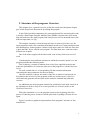
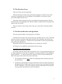
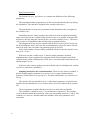
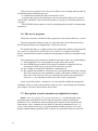
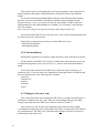
Figure 1 provides a graphical representation of the program’s structure of four
main blocks.
9
The ensuing description of the code’s structure will be divided into three parts:
Firstly we describe the Input Preparator, or the part of the program that is directly
above the User’s Program. Secondly, we describe the Bayesian Layer which does all
the extra work needed to run a simulation across the different scenarios. Thirdly, we
address the parallel algorithms of the PMC driver and lay out the algorithmic structure
of the driver.
Bayesian Layer
Input Preparator
Workload
Controller
User’s code
Fig.1 - Layout of the program’s components and main routines.
2.1 The Input Preparator
This part of the program begins by reading two external files.
These files contain information on the parameters of the user model that are to
vary during the MC simulation, what distribution they should have, the total number
of runs to be performed, the maximum number of model parameters that are to be
varied during the simulation, etc.
Having read these files, the program goes through the list of user parameters that
are to vary and does a sampling of each of the desired distributions. The values
generated are stored both externally (in a file) and internally (in a matrix).
10
2.2 The Bayesian Layer
This part of the code runs optionally.
The bayesian layer is built on top of the input preparator. It chooses one of the
scenarios at random from a list according to its probability of occurrence (both
previously supplied by the user).
Once that is done, the bayesian layer just supplies the input preparator with the
input file name corresponding to the chosen scenario so that the latter can prepare the
input for the user model.
The user model is run as many times as the user wants before choosing another
scenario.
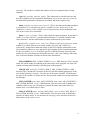
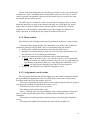
2.3 Parallel architecture and algorithms
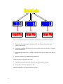
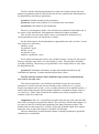
The most general outline of the program is as follows:
The PMC driver itself is run on one node only (called the master node). This node
prepares a matrix with all the input data needed for the simulation and controls the
size of the next workload (i.e., fraction of the total number of runs to be performed)
and which node should get it.
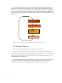
Each node executes its workload and writes its output to a local file.
See Figure 2 for a graphical representation of this concept.
Algorithm of the Input Preparator
Increasing a little the detail of the description, here is a rough listing/fluxogram of
the input preparator (for the sake of simplicity, we assume that there is no simulation
across scenarios – i.e., the bayesian layer is inactive). Please keep in mind that the
PMC driver part of the code is run on one node only.
1. The program reads the name of the file containing all the constant values for
the user model.
2. It makes the same number of copies of that file as there are nodes involved in
that particular job. Each node will access its own copy of the input file during
the MC simulation. (These files and any other files mentioned in this manual
are kept in the same directory as the executables)
11
…
Fig. 2- Conceptual organisation of a MC simulation in a parallel environment.
3. Reads the file containing the parameters for the distributions of the input
values of the model.
4. Generates a random distribution for each variable and stores it both in a matrix
and an external file.
5. Generates the output files to which each node will write its output (one file per
node).
6. Informs each node of which runs it should run.
(All nodes execute the next two steps)
7. Calls the user model and runs it for the specified number of times.
8. Every node writes its output to its file.
(Master node takes over again.) Returns to step 6.
12
Algorithm of the Bayesian Layer
Now let us see what the bayesian layer does, when activated. (There are some
terms that the reader might not be familiar with, these are explained in ref. [1] and
references therein.)
The bayesian layer is built on top of the input preparator (the code that was
explained in the previous paragraph) and is run only on the root node.
The following is nested in a loop, that runs as many times as the user wishes.
1. Read an input file with information necessary for the bayesian simulation: the
total number of scenarios and the probabilities for each scenario, together with
names for the files with information regarding the input values for each
scenario.
2. Random choice (according to the probabilities specified) of a scenario.
3. Call the input preparator.
4. Return to the beginning of the loop (this time skipping the reading of the
bayesian input file).
13
14
3. Description of the algorithms
3.1. Inputs required from the user
Before compiling the program, the user should supply the following set of
switches, numerical parameters and file names (by writing them in the suitable
parameter declaration files).
In the paragraphs to come we shall describe the contents and the format of the
following files:
•
•
•
•
user_parameters_bayes.inc
user_parameters.inc
mcdinputb.dat
mcddist.dat
Bayesian layer files:
The “include file” called user_parameters_bayes.inc contains the definition of the
following variables:
(De)Activation of the bayesian layer: variable sbayes (the value 1 activates the
layer, value 0 deactivates it).
The default name for the files with the constant values for the model and the name
of the file with the distribution parameters for the model should be supplied (by
assigning them to the variables constfile and distrifile, respectively).
In its first line, the input file for the bayesian layer (mcdinputb.dat) should contain
the total number of micro-scenarios.
Each of the following lines should contain (one line per micro-scenario):
(position 1 in the line) the probability of that specific micro-scenario,
(position 13) the name of the file with the distribution parameters for that microscenario, and
(position 34) the name of the file with the constant values corresponding to that
micro-scenario.
15
Input Preparator files.
The include file user_parameters.inc contains the definition of the following
parameters:
The maximum number of parameters (in the user model) that should vary during
the simulation. This should be assigned to the variable called ivars.
The total number of runs to be performed on this simulation; this is assigned to
the variable iruns.
Sometimes the user wants to analyse the behaviour of the model by performing
some runs with only one variable being varied at a time. It is possible to do this with
this driver, the only thing the user has to do is to set the variable sim to 1. The driver
will set up a set of simulations that will develop as explained below.
The program will vary the first variable only in the list in distrifile for #iruns on
the first simulation, then it will vary the second parameter only in the list in distrifile,
and so on until it has varied the last parameter given in distrifile.
So the total number of runs actually performed will not be the one stored in iruns,
but: #sim * #iruns.
If the user sets the variable sim to 2, after the single parameter variation
simulations have been completed, the program does a final simulation with all the
variables being varied simultaneously. If the user is just interested in this last case, he
should assign 0 to sim.
If the user only wants to perform one run with the code, he should put the varibale
switch to 0, otherwise it should be 1.
Sampling method for the random numbers. There are two choices available: a
pseudo-random number generator (set sgenop to 0) or a quasi-random number
generator (Sobol indices) (set sgenop to 1). For more information, see references [1]
and [2].
The switch sinfilemat should be set to 1 if the input preparator is to generate the
numbers for the simulations, or to 0 if these values are to be loaded from an external
file.
The next program variables that the user has to set deal with correlations.
The variable key should be set to 1 for correlations (0 otherwise). The variable
correlat should contain the correlation value (any real number between –1 and 0). The
variables var1 and var2 should contain the numbers of the user parameters to be
correlated.
16
The file with the distribution parameters (mcddist.dat) should contain the total
number of parameters that are described in the file first, and then the information for
the distributions (one line per parameter):
(position 1) number assigned to the parameter.
(position 4) name of the variable as it is defined in the user model.
(position 64) code name for the distribution.
The user is encouraged to make a list of all the user parameters that might vary in
the course of his simulations. Each parameter should be assigned a number.
This way the user can easily add or remove user parameters from the list of
varying parameters from one simulation to another.
See the following list for the distributions supported by the code (version 1.0) and
their respective code names,
uniform- unifm
log-uniform- logun
normal- norml
log-normal- logno
negative exponential- expon
If one wants to temporarily remove one variable from the varying list, this can be
done by using the code word const and writing its value. This procedure should be
avoided if possible. The memory saving alternative is to simply delete its entry from
the distributions file.
(position 67) minimum, maximum, average and standard deviation for the
distribution in question. Commas should separate these values.
The file with the constant values should be kept exactly as usual when the
user code is run only once.
The code can introduce a user-defined correlation between any two modelparameters. In order to do this, the user should set the variable key to 2, put the
desired correlation value on the correlat variable (this has to be a number between –1
and 0) and tell the program which variables should be correlated (with the values of
var1 and var2). These values should be the numbers previously assigned to each
variable on the file mcddist.dat.
Output data. Since it’s very difficult to predict what the user will want, the PMC
driver does not impose any particular format. The user has to decide what output is to
be written to the file created at the beginning of the Input Preparator routine. The
default name for the output file is mcdout* (where the wildcard stands for a number
that is the same as the node number to which the file belongs).
The user should keep in mind that the amount of output generated in typical MC
simulations is considerable.
17
There is an additional set of output files generated by the driver. These contain the
run times for each run and they are called mcdtimeout* (where the wildcard again
stands for a number equal to the node number).
3.2. The input preparation
This part of the code performs several tasks: it makes copies of the files with the
constant parameters for the simulation, produces the output files for each node and
samples the input values for the model parameters chosen by the user.
The routine begins by making the copies of the file with the constant parameters
for the simulation. This should be exactly the same file as the one usually used by the
user's model.
The code generates a different target name for each of the files. Each copy will be
read by just one of the nodes. The names of the files start with the string mcdconst
then have a code specific to each file.
Almost the same procedure is carried out to produce the output files, with the
difference that they are all empty. They are all called mcdout followed by a number to
distinguish between them.
Warning: avoid using any files that contain the string mcdconst or mcdout, to
avoid possible conflicts with the simulation.
All the nodes open their corresponding file.
From now on, only node 0 (zero) does all the work.
Two files are opened: the file with the distribution parameters for each of the
model variables (called mcddist.dat) and a file to contain the values generated from
the sampling (called mcdmdist.dat).
If the quasi-random numbers option is chosen, there is a call to the subroutine that
generates the numbers, in this case a routine obtained from the NEA (Nuclear Energy
Agency) data bank called lptau.f (package ID: IAEA1260)/02). This routine uses
Sobol indices to perform the sampling of a quasi-random uniform sequence between 0
and 1. The values are stored in a matrix (matrixlpt) (see [2] and [5]).
The next part is included in a loop that runs for #ivars times. The program reads
the file mcddist.dat, interprets which distribution is required for each particular model
parameter and uses some sub-routines to sample the required distribution for the
number of times specified in the variable iruns. (See [2] for a description of the
sampling routines).
18
In the event that the user wishes to do so, the program will then introduce a
correlation between any two input variables (see [6] for details on the method used).
It is also possible for the program to read a file with pre-defined values for the
matrix mdist.dat.
The values resulting from the sampling are written to the output file mcdmdist.dat
and in the matrix mdist.
The master node sends the contents of mdist to all the other nodes. At the end of
each simulation, each node writes the output to their local file.
Finally, all files are closed and a small UNIX script cleans all temporary files.
3.3. The workload controller
Initially the master node assigns a predefined workload to each node.
The master node awaits a call from one of the other nodes to request another
workload and when it finally gets one, it tells that node which run(s) it should run
next (what we call a workload). As soon as a node has finished its workload it
informs the master node that it needs another workload. This is done until all iruns
are completed.
3.4. The bayesian layer
The bayesian layer is run as many times as the user wants.
The routine called bayes is very simple. First it reads a file with the total number
of scenarios, the probability assigned to each of them and the files with the
information to simulate each scenario.
It makes a random selection among the scenarios available, then informs the input
preparator of the selection.
3.5. The interface between the input preparation and the user
code
The input preparator supplies the user model with the following information (the
variable concerned is shown in brackets):
- Number of runs that each node will run the model (load),
- Total number of model parameters that are going to vary in the simulation
(ivars),
- Total number of runs (iruns),
19
(These last two parameters are only used to define some working matrixes that are
needed during the simulation process),
- A variable that contains the rank of each node (rank),
- A pointer that chooses the right input value for the model whatever the current
status of the simulation ('only one model parameter varying' or 'all model parameters
varying'),
- The FORTRAN unit number of the file containing all the model's constant input
parameters.
3.6. The user's program
Firstly the user must re-define his/her program as a sub-routine called user_model.
The most important changes to the user code take place in the subroutine where
all the input parameters are assigned their values for each run.
We assume that there is a single routine in the model that reads the usual input file
(by ‘usual’ we mean the file used by the user’s before it is coupled to the PMC
driver), and that all the model’s parameters and program switches are assigned by this
routine.
The original part of the subroutine should be kept intact with a few small changes:
i) there should be a few extra parameters in the call to this routine,
ii) the FORTRAN unit number of the input file should be changed to the one
passed by the PMC driver (referred at the end of the section),
iii) any writing to external files should be commented out,
iv) the original code should be enclosed in an if statement that allows the constant
file to be read just once per simulation. (If any of the input variables is re-used
later in the code, then it is safer to re-initialise the values at the beginning of
each run, i.e., one should not enclose the code in this if statement).
At the end of the routine, a small piece of code should be added that assigns the
stochastic values to each of the parameters that are to be varied during the simulation.
See Chapter 4 for more detail on how this is done.
3.7. Description of each subroutine (in alphabetical order)
distri (iruns, ivars, ndist, IN1, genop, matrixlpt, i) – Is called from the input
preparator part of the PMC driver. It reads the input file with the distribution
parameters -IN1- and decides which sampling sub-routines to call to generate the
input matrix. Ndist contains the code name for the chosen distribution (see 3.1).
genop is the option for the type of (pseudo)random number generator. If it is the
pseudo-random number generator that is chosen, the generated values are stored in
20
matrixlpt. The variable i contains the number of the user parameter that is being
sampled.
expo (dist_min,dist_max,dist_mean) - This subroutine is called from distri and
does the sampling for an exponential distribution. dist_min,dist_max,dist_mean are
the distribution parameters (minimum, maximum and mean, respectively).
iman (iruns,key,correlat,vector1,vector2) –This is the sub-routine that introduces
a correlation of correlat between any two variables vector1 and vector2, if the
variable key is set to 0. The variable iruns is only necessary for the definition of the
size of the vectors to be correlated.
lptau (i, ivars, vectorlpt) - This is called from the input preparator. It generates a
vector (vectorlpt) with ivars’ pseudo random numbers. i is an index number (that
varies between 1 and the total number of runs) needed for the lptau routine.
ip (distrifile, constfile, ierror, rank, size) - What we call input preparator in this
manual. It is called from the mcd (main) routine. distrifile and constfile are,
respectively, strings that contain the names of the files with the information for the
user parameters that are to vary and the file that contains all the constant parameters
for the user model. ierror is a variable specific to MPI and usually stores the code
number for the errors that occur during the run time. rank is the ranking of the node.
Size is the total number of nodes involved in the simulations.
MPI_BARRIER (MPI_COMM_WORLD, ierror) - MPI function. This is used to
make sure all the nodes are running in the same stage of the program. No node will
continue running until all nodes reach this part of the program.
MPI_BCAST (constfile, 20, MPI_CHAR, 0, MPI_COMM_WORLD) - MPI
function. This ”broadcasts” the name of the file with the constant parameters of the
user model (stored in constfile), 20 is the size of the name and MPI_CHAR denotes
the type of the variable. O means that it is the root node (ranked zero) that broadcasts
the message.
MPI_GATHER (vout, index, MPI_INTEGER, mout, index, MPI_INTEGER, 0,
MPI_COMM_WORLD, ierror) - MPI function. The root node (rank 0) gathers the
contents of the vector vout (of integers) from all the other nodes and stores it in
matrix mout. vout which has size index.
MPI_SCATTER (mdist, ncounts, MPI_REAL, vector, ncounts, MPI_REAL, 0,
MPI_COMM_WORLD, ierror) - MPI function. The root node (rank 0) distributes
portions of matrix mdist, of size ncounts (of real type), to be stored on each of the
other nodes on the vector vector.
21
norm (dist_min, dist_max, dist_mean, dist_stan) - This subroutine is called from
distri and does the sampling for a normal distribution. dist_min,dist_max,dist_mean,
dist_stan are the distribution parameters (minimum, maximum, mean and standard
deviation, respectively).
readb (vect_prob, n_sce, input_file1, input_file2, in1) - This routine is called
from routine bayes and it reads the input file with all the information concerning the
bayesian layer (number of scenarios -n_sce -, probabilities for each scenario
-vect_prob -, names for the input files for each scenario -input_file1 and input_file2,
etc.).
selection (vect_prob, n_sce1, sel, trial) - Called from readb subroutine; it makes
the random selection of the scenario for the simulation.
system ("clean") - Unix system script that cleans all the temporary files created
during the simulation.
system ("spawn") - Unix system script that creates the input file with the constant
parameters for all the nodes.
unif (dist_min, dist_max) - This sub-routine is called from distri and does the
sampling for a uniform distribution. dist_min,dist_max, are the distribution
parameters (minimum and maximum, respectively).
user_model (load, ivars, iruns, ncounts, vector, rank, master, nnodes, fot2, index,
vout, mout, switch, in2) - User_model stands for the name of the user program. It is
called from the input preparator.
22
4. Putting the PMC driver together with the user code
4.1 Machine and environment requirements
So far only a Unix version of the code is available and tested. Such specificity of
working environment only involves two small system scripts. One of these
"multiplies" the files containing the constant values for the simulation and the other
deletes all the temporary files.
More specifically, the first script reads a temporary file (mcdname) with the name
of the original file that is to be copied, then it copies its contents into a number of files
whose name begins with the string input and then it finishes with a number. The total
number of files to generate is contained in another temporary file called mcdnr.
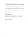
The script’s contents are reproduced here:
#! /bin/tcsh
foreach n ({`cat nr`})
cp `cat name` input$n
end
Warning: The first line says that this script should be run within the tc shell by
stating the path where this shell start up command should be located (/bin/tcsh). This
path might be different from one system to another (/usr/local/bin/tcsh is a common
alternative).
The second script simply contains the command: rm -f input*.
There’s a version of these srcipts for the bash shell too.
The code has been developed in a parallel machine located at the Royal Institute
of Technology in Stockholm, Sweden. The machine is an IBM SP2, and the nodes’
architectures are the normal RS2000-type workstations (see the Internet site
http://www.pdc.kth.se/compresc/machines/strindberg.html for more details).
The code was tested in a workstation network environment located at Bath
University. The workstations are different models of high-end SUN stations. It was
also used in a cluster of Alpha workstations at the Department of Physics at
Stockholm University.
Using the message-passing model allowed the simulations to be parallelized.
23
This model consists in expanding the usual serial programs with a collection of
library functions that enable communication to take place between the different
nodes.
We use the international standard library known as the MPI (Message Passing
Interface) and users should have that library installed in their machine (see the
Internet site http://www.erc.msstate.edu/mpi/ for more detail on MPI). Different
implementations of the MPI standard are available, free of charge, on the Internet.
(See for example,
http://www.psc.edu/general/software/packages/mpich/mpich.html.old).
At the head of the PMC driver's code one can see the include statement that loads
the library mpif.h for Fortran code.
So the basic requirements necessary to run the PMC driver are:
- UNIX based machines,
- MPI implementation.
4.2 Code installation
Install all the programs in a separate, empty directory, along with the user model.
All the output of the PMC driver will be created in the same directory as the one
in which the program is run, no use of local (i.e., local to each node) hard disks is
made.
At the end of the simulation, the PMC driver performs some cleaning up of
temporary files. If for any reason, the simulation is interrupted before its natural end,
then you should remove the following files by hand:
mcdinput*
mcdtimeout*
mcdout*
mcdname
mcdnr.
4.3 Changes to the user code
One of the main goals in developing the PMC driver was that it should require a
minimum of change to the user code. There are some changes that are inevitable,
though, especially when the PMC driver itself is coded in Fortran 77.
One rule that is valid for any of the programs is that almost all the reading
(excluding the reading from the read routine) and all the writing to/from files should
be commented out. The PMC driver should control all these activities with its predefined input and output files.
24
So one of the main things the user should keep in mind is to be very careful with
external files. This is something that is unavoidable when one tries to use a ”serial”
code in a parallel environment, otherwise all the nodes will try to write to the same
file and the result could be messy!
The PMC driver is written in a such a way that the user does not have to worry
about the input files (as long as the original code only uses ONE input file, and as
long as this is read in a single routine). All the output to external files, from the
original user code, should be commented out (see the example in Chapter 5), or,
better expressed, be redirected to the output file defined in the driver.
4.3.1. Main routine
Here follows a list of changes that must be performed on the user’s main routine.
1- Substitute the program header with "subroutine user_model" and include the
parameters passed to it by the PMC driver (as described in the last chapter).
2- Define all the variables and matrices passed by the PMC driver.
3- Introduce a loop that should go from 1 to load. This loop should enclose all
the code that is to be run during the simulation.
4- Add a few parameters do the subroutine calls to input and output:
• Input: rank of the node (rank), a few switches (master, switch) that avoid
having to read the file with the constant values in every run, and finally the
total number of parameters that are to vary during the simulation (ivars).
• Output: the logical name defined by the PMCD for the output file.
5- At the end, the statement stop should be changed to return.
4.3.2. Assignment (read) routine
The sub-routine that does the initial assignment of the model's parameters should
get some additional parameters when it is called. Most of these have already been
described at the end of the last chapter, they are:
- The vector containing the input values for the model parameters that are going to
vary during the simulation (stored on the vector vector),
- The total size of the vector vector (ncounts),
- The ranking of the current node (rank),
- Master, when the user is doing simulations with a single parameter varying at a
time, it is this variable that keeps track of which parameter should vary in each
simulation.
- The number of model parameters that are going to vary during the simulation
(ivars),
- The logical unit number for the input file (stored in the variable in2).
25
Apart from the usual changes to make the extra parameters (in the last list)
available to the routine, one can introduce the following if statement, that should
enclose all of the original code in the routine:
if (NRUN.eq.1) then
NRUN stands for the variable that controls the loop described in point 3 in the
previous chapter.
This last change keeps the code from reading the same input file in every run. It
saves some run time, but it should only be used when the user is sure that the values
from the file are not needed in the subsequent runs.
At the end of the routine (and after the end of the if statement just mentioned), the
following code should be added (with some dummy variables):
if (switch.eq.1) then
if (sim.eq.0.or.(sim.eq.2.and.master.eq.ivars+1)) then
pointer=1
endif
if (check_in(1).eqv..true.) then
INPUT_PARAMETER1=mdist(pointer,nrun+run-1)
pointer=pointer+1
write(fot3,'(D13.7)') INPUT_PARAMETER1
endif
INPUT_PARAMETER1
is a dummy variable name that stands for the typical model
parameters that are to be varied during the simulation. Master is a variable that keeps
track of which case is being run (as explained in Section 3.1).
The vector check_in is a vector that keeps track of which user parameters are
varying in that particular simulation (when the input preparator reads the mcddistr.dat
file, it checks which parameters are listed there and which are not).
The user is encouraged to make a list of all the user parameters that might vary in
the course of his/her simulations. Each parameter should be assigned a number and
there should be a piece of code (like the one written in yellow above) for each user
parameter. In this way the user can add or remove user parameters from the list of
varying parameters from one simulation to without trouble.
The write statement simply stores the input value in the output file. The user is
free to keep this line of code or to comment it out.
It is this part of the code that actually updates the model parameters from one run
to the next.
26
4.3.3. Output subroutine
The user should comment out all the original reading/writing from/to external
files. Then he/she should write the values he/she is interested in to the file descriptor
number fot3.
Here is an example:
write(fot3,'(D13.7)') OUTPUT_PARAMETER1
OUTPUT_PARAMETER1
stands for a common output variable name.
4.4 Changes to the PMC driver
There are no changes to be made to the code of the PMC driver.
In the input files one must decide between the options of and determine values for
the PMC driver parameters, but this is not specific to the grafting of the PMC driver
to the user model. These are things that are to be when working with the PMC driver.
In Chapter 6 we make a list of the things that must be kept in mind before hitting the
RETURN key on the keyboard.
27
28
5. Practical Example 1: Making a parallel run of a Monte
Carlo simulation of a simple one-dimensional transport
model with retardation
This is a sample file for the bayesian input file:
3
0.30
0.40
0.30
norm1.inp
norm2.inp
expo.inp
const
const
const
The first number states the number of micro-scenarios.
The subsequent lines describe the probabilities of each microscenario and give the
names of the input files.
Here is an example of the file const.dat with all the constant parameters of the
user model:
18
1.0
4.3 0.231E-5
3.0
3.0
10.
The number on the first line denotes the number of space points that is to be
sampled from the solution.
The second line respectively contains: the initial concentration, the dispersion
coefficient, the advective velocity, the retention coefficient, the time at which the
solution is evaluated and the space increment.
Here is a typical file containing the variable distribution parameters for the user’s
program.
5
10
20
30
40
50
60
************************************************************
********************INPUT PARAMETERS************************
************************************************************
END OF COMMENTS
Number of user parameters that are to vary in the Mc run : 2
1 ALFX GEO : Dispersion coefficient [m]......: unifm 1.,5.
2 RF GEO : Retention coefficient
[-].........: expon 2.,10.,0.1
First we have a number to identify the variable, then the variable name, some
comments describing the variable and at the end the code word for the distribution of
its values and the parameters for that distribution.
29
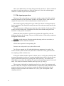
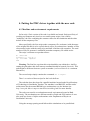
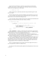
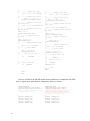
Next we show the main routine of the user code, before (in the column on the left)
and after (in the column on the right) being coupled to the PMC driver.
(We have marked the parts that are changed).
program ad
C
CODE FOR EVALUATING 1-D DISPERSION
WITH RETARDATION
C
C
subroutine user_model (mdist,
load,ivars,iruns,check_in,
& rank,master,switch,in2,sim,fot3,fot4,run)
C
CODE FOR EVALUATING 1-D DISPERSION
WITH RETARDATION
C
C
Integer nrun,j
INTEGER iruns,ivars,rank,master
INTEGER switch,in2,sim,fot3,fot4
INTEGER load,run
Double precision mdist(ivars,iruns)
logical check_in(ivars)
DIMENSION C(50)
DIMENSION C(50)
index=1
pointer=1
do nrun=1, load
C
C
READ INPUT DATA
C
OPEN(unit=10,file='ind.dat',status='OLD')
OPEN(unit=11,file='out.dat',status='NEW')
C
C
C
C
C
C
READ(in2,100)NX
WRITE(11,100)NX
READ(in2,110) CO,ALFX,VX,RF,TYR,DELX
C
WRITE(11,110) CO,ALFX,VX,RF,TYR,DELX
C
C
C
WRITE(11,110)
WRITE(11,110)
READ INPUT DATA
OPEN(unit=10,file='ind.dat',status='OLD')
OPEN(unit=11,file='out.dat',status='NEW')
if(nrun.eq.1) then
READ(in2,100)NX
WRITE(11,100)NX
READ(in2,110) CO,ALFX,VX,RF,TYR,DELX
WRITE(11,110) CO,ALFX,VX,RF,TYR,DELX
WRITE(11,110)
WRITE(11,110)
end if
if (switch.eq.1) then
if
(sim.eq.1.or.(sim.eq.ivars+1.and.master.eq.ivars+1)) then
ALFX= mdist(pointer,nrun+run-1)
pointer=pointer+1
RF= mdist(pointer,nrun+run-1)
pointer=pointer+1
endif
endif
C
C
TSEC=TYR*365.0*86400.0
X=0.0
C
C
C
CALCULATE CONCENTRATIONS
DO 200 I=1,NX
X=X+DELX
200
C(I)=(CO/2)*ERFC((RF*XVX*TSEC)/(2*SQRT(ALFX*VX*TSEC*RF)))
C
C
WRITE RESULTS
C
WRITE(11,120)TYR
WRITE(11,110)(C(I),I=1,NX)
30
TSEC=TYR*365.0*86400.0
X=0.0
C
C
C
CALCULATE CONCENTRATIONS
DO 200 I=1,NX
X=X+DELX
200
C(I)=(CO/2)*ERFC((RF*XVX*TSEC)/(2*SQRT(ALFX*VX*TSEC*RF)))
C
C
WRITE RESULTS
C
C
WRITE(11,120)TYR
C
WRITE(11,110)(C(I),I=1,NX)
do j=1,NX
write(fot3,'(D13.7)') c(j)
end do
end do
100 FORMAT(I5)
110 FORMAT(6G10.2)
120 FORMAT(F5.0, ' YEARS')
return
END
end do
100 FORMAT(I5)
110 FORMAT(6G10.2)
120 FORMAT(F5.0, ' YEARS')
return
END
31
32
6. Practical Example 2: Making a parallel run of a Monte
Carlo simulation with the GTM1 code
The reader should be familiar with report [1] if he/she is to understand the detail
of this chapter.
The sample file for the bayesian input file is:
6
0.3
0.15
0.2
0.1
0.15
0.2
dist1
dist2
dist3
dist4
dist5
dist6
input1
input2
input3
input4
input5
input6
The first number states the number of micro-scenarios.
The subsequent lines respectively describe the probability of each micro-scenario
occurring, and give the name of the input file containing the distribution and the
constant parameter.
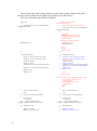
Here is an example of the file mcdconst.dat with all the constant parameters of the
user model.
********************************************************************************
********************************************************************************
*
*
*
G.T.M - 01 (Geosphere Transport Model - 1)
*
*
========== *
********************************************************************************
*
*
*
PEDRO PRADO HERRERO
*
*
Centro de Investigaciones Energeticas
*
*
Medioambientales y Tecnologicas (CIEMAT) *
*
Instituto de Tecnología Nuclear (ITN)
*
*
Avda.
Complutense, 22
*
*
- 28040 - Madrid
(ESPAÑA)
*
*
*
********************************************************************************
*
*
*
RUN CASE :
*
*
PSACOIN Level E (PSAC User Group - OECD/NEA)
*
*
--------------*
*
*
*
REFERENCES:
*
*
1. PSACOIN LEVEL E INTERCOMPARISON
*
*
Probabilistic System Assessment Code (PSAC) User Group *
*
NEA/OECD (1989)
*
*
*
********************************************************************************
END OF COMMENTS
0...5....1....5....2....5....3....5....4....5....5....5....6....5....7....5....8
FORTRAN NAME ID
VARIABLE DESCRIPTION
UNITS
VALUE
===============
====================
=====
=====
33
MXFL
CP : Option for max-flux
SPACTL
CP : Option for space manag.
TIMCTL
CP : Option for time manag.
minpxx
cp : Option min.spa.poin/ly
minnpx
cp : min nº space point/lay.
NAO
CP : Option for analy. sol.
DTHGST
CP : Highest time step
CTRUN
CP : Trunca. value for conc.
DRINKR
BIO : Drinking water require.
----> CHAIN NUMBER 1 -------------NEL (1)
GTM : Number of nuclides
BNAME(I -129)
GTM : Name of nuclides
ALAMB(I -129)
GTM : Decay constant
RET (I)
GEO : Retardation coefficient
C0
(I -129)
NFL : Initial inventory
DOSECF(I -129)
BIO : Dose Conversion factor
----> CHAIN NUMBER 2 -------------NEL (2)
GTM : Number of nuclides
BNAME(NP-237)
GTM : Name of nuclides
ALAMB(NP-237)
GTM : Decay constant
RET (Np)
GEO : Retardation coefficient
C0
(NP-237)
NFL : Initial inventory
DOSECF(NP-237)
BIO : Dose Conversion factor
BNAME(U -233)
GTM : Name of nuclides
ALAMB(U -233)
GTM : Decay constant
RET (U )
GEO : Retardation coefficient
C0
(U -233)
NFL : Initial inventory
DOSECF(U -233)
BIO : Dose Conversion factor
BNAME(TH-229)
GTM : Name of nuclides
ALAMB(TH-229)
GTM : Decay constant
RET (Th)
GEO : Retardation coefficient
C0
(TH-229)
NFL : Initial inventory
DOSECF(TH-229)
BIO : Dose Conversion factor
----> LAYER 1 --------------------DIFFM (1)
GEO : Molecular diffusion
DISPC (1)
GEO : Dispersion coefficient
----> LAYER 2 --------------------DIFFM (2)
GEO : Molecular diffusion
DISPC (2)
GEO : Dispersion coefficient
*******>> DATA RUN-1 <<************
CONTIM
NFL : Containment time
STREAM
BIO : Stream flow rate
----> LAYER 1 --------------------XPATH (1)
GEO : Geosphere pathway
VREAL (1)
GEO : Interstitial velocity
----> LAYER 2 --------------------XPATH (2)
GEO : Geosphere pathway
VREAL (2)
GEO : Interstitial velocity
---------> CHAIN 1 ---------------NOUT
GEO : Nº time output selected
TOUT (1)
GEO : Time point selected
RLEACH
NFL : Leach rate
FACM (1)
GEO : * Factor for retention
FACM (2)
GEO : * Factor for retention
---------> CHAIN 2 ---------------NOUT
GEO : Nº time output selected
TOUT (1)
GEO : Time point selected
TOUT (2)
GEO : Time point selected
TOUT (3)
GEO : Time point selected
RLEACH
NFL : Leach rate
FACM (1)
GEO : * Factor for retention
[ - ]
[ - ]
[ - ]
[ - ]
[ - ]
[ - ]
[ yr ]
[mols]
[m**3/yr]
.TRUE.
.FALSE.
.FALSE.
.true.
5
2
70000.
1.0E-10
0.73E+0
[ - ]
[ - ]
[1/yr]
[ - ]
[mols]
[Sv/mol]
1
I -129
4.41E-8
1.
100.
5.60E+1
[ - ]
[ - ]
[1/yr]
[ - ]
[mols]
[Sv/mol]
[ - ]
[1/yr]
[ - ]
[mols]
[Sv/mol]
[ - ]
[1/yr]
[ - ]
[mols]
[Sv/mol]
3
NP-237
3.24E-7
100.
1000.
6.80E+3
U -233
4.37E-6
10.
100.
5.90E+3
TH-229
9.44E-5
100.
1000.
1.80E+6
[m**2/yr]
[m]
0.
10.
[m**2/yr]
[m]
0.
5.
[y]
[m**3/yr]
100.
3.0E+5
[m]
[m/yr]
100.
1.0E-1
[m]
[m/yr]
50.
1.0E-1
[-]
[yr]
[1/yr]
[ - ]
[ - ]
1
9.55E+2
1.0E-2
1.
1.
[-]
[yr]
[yr]
[yr]
[1/yr]
[ - ]
3
5.24E+4
6.63E+4
3.07E+5
1.0E-5
3.
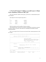
Here is a typical file showing the distribution parameters for the user program’s
parameters that are to vary during the simulation.
************************************************************
********************INPUT PARAMETERS************************
************************************************************
END OF COMMENTS
5
10
20
30
40
50
60
Number of runs........................................(I2): 10
Number of variables...................................(I2): 10
Number of constants...................................(I2): 53
34
CONTIM
NFL : Containment time
[y]......: norml
0.,1000.,500.,200.
RLEACH (1)
NFL : Iodine leach rate
[1/yr]...: norml
0.00075,0.0125,0.005,0.0025
RLEACH (2)
NFL : Chain leach rate [1/yr]...: norm
0.0000075,0.000125,0.00005,0.000025
VREAL (1)
GEO : Interstitial velocity
[m/yr]...: norml
0.0075,0.125,0.05,0.025
XPATH (1)
GEO : Geosphere pathway
[m]......: norml 0.,600.,300.,100.
RET (I)
GEO : Retardation coefficient
[ - ]....: norml 0.,9.,3.,1.
FACM(2,1)
GEO : Factor for retention
[-]......: norml
0.,34.,16.5,6.75
VREAL (2)
GEO : Interstitial velocity
[m/yr]...: norml
0.0075,0.125,0.05,0.025
XPATH (2)
GEO : Geosphere pathway
[m]......: norml 0.,250.,125.,37.5
STREAM
BIO : Stream flow rate
[m**3/yr]: norml
0.,2000000.,1000000.,500000.
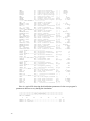
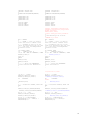
Next we show the main routine of the user code, before (the column on the left)
and after (the column on the right) being coupled to the MC driver. Those parts that
are changed are highlighted).
PROGRAM GTM
C
C
C
C
INCLUDE 'CPARAM.INC'
INCLUDE
INCLUDE
INCLUDE
INCLUDE
INCLUDE
INCLUDE
INCLUDE
'COTISP.INC'
'CNUCNA.INC'
'CNUCLI.INC'
'CNARFL.INC'
'CFARFL.INC'
'CBIOSP.INC'
'COUTPS.INC'
CHARACTER TIM*8
LOGICAL START
LOGICAL TIMCTL
LOGICAL SPACTL
subroutine
user_model(mdist,load,ivars,iruns,c
heck_in,
rank,master,switch,in2,sim,fot3,fot
4,run)
C
INCLUDE 'CPARAM.INC'
C
INCLUDE 'COTISP.INC'
INCLUDE 'CNUCNA.INC'
INCLUDE 'CNUCLI.INC'
INCLUDE 'CNARFL.INC'
INCLUDE 'CFARFL.INC'
INCLUDE 'CBIOSP.INC'
INCLUDE 'COUTPS.INC'
C
CHARACTER TIM*8
C
LOGICAL START
LOGICAL TIMCTL
LOGICAL SPACTL
INTEGER iruns,ivars,
,rank,master
INTEGER fot3,fot4,switch
Double precision
mdist(ivars,iruns)
integer load,in2,sim,run
logical check_in(ivars)
C
START = .TRUE.
C
C.....run loop
C
DO 10 NRUN = 1,MXNRUN
C
C........chain loop
C
DO 20 NCHAIN = 1,MXNCHN
C
C...........read input values
C
CALL R E A D
(NRUN,NCHAIN,NOUT,MXFL,DTHGST,
START,NAO,CTRUN,SPACTL,TI
MCTL)
START = .TRUE.
C
C.....run loop
C
DO 10 NRUN = 1,load
C
C........chain loop
C
DO 20 NCHAIN = 1,MXNCHN
DO 20 NCHAIN = 1,MXNCHN
C
C...........read input values
C
CALL R E A D
(NRUN,NCHAIN,NOUT,MXFL,DTHGST,
START,NAO,CTRUN,SPACTL,TIMCTL,
mdist,check_in,rank,master,switch,i
vars,iruns,in2, sim,fot3,run)
35
C
C...........compute space step
C
CALL
S P A C S E (SPACTL)
C
C...........compute time series
C
CALL
T I M E S E
(NCHAIN,NOUT,DTHGST,TIMCTL)
C
C...........compute fluxes from
the near field
C
CALL
N E A R F (NCHAIN,nao)
C
C...........compute fluxes from
the far field
C
CALL G T M 1
(NCHAIN,CTRUN,MXFL,NOUT)
C
C...........compute analytical
solution
C
CALL
A N A S O L
(NAO,NCHAIN,NOUT)
C
C...........compute maximum dose
C
CALL
B I O S (NCHAIN)
C
C...........print outputs
C
CALL
O U T P U T
(NCHAIN,NOUT,MXFL)
C
C........end of chain loop
C
20
CONTINUE
C
C.....end of run loop
C
10
CONTINUE
C
C...........compute space step
C
CALL
S P A C S E (SPACTL)
C
C...........compute time series
C
CALL
T I M E S E
(NCHAIN,NOUT,DTHGST,TIMCTL)
C
C...........compute fluxes from the
near field
C
CALL
N E A R F (NCHAIN,nao)
C
C...........compute fluxes from the
far field
C
CALL G T M 1
(NCHAIN,CTRUN,MXFL,NOUT)
C
C...........compute analytical
solution
C
CALL A N A S O
L(NAO,NCHAIN,NOUT)
C
C...........compute maximun dose
C
CALL
B I O S (NCHAIN)
C
C...........print outputs
C
CALL
O U T P U T
(NCHAIN,NOUT,MXFL,fot3)
C
C........end of chain loop
C
20
CONTINUE
C
C.....end of run loop
C
10
CONTINUE
FORMAT(E13.5)
C
STOP
RETURN
END
STOP
END
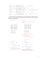
Now we will show the READ routine before and after it is adapted to the PMC
driver. Again, those parts that are changed are shown in colour.
SUBROUTINE READ
(NRUN,NCHAIN,NOUT,MXFL,DTHGST,
START,NAO,CTRUN,SPACTL,TIMCTL)C--------------------------------------------------------C
INCLUDE
C
INCLUDE
INCLUDE
INCLUDE
INCLUDE
36
'CPARAM.INC'
'CNUCNA.INC'
'CNUCLI.INC'
'CNARFL.INC'
'CFARFL.INC'
SUBROUTINE READ
(NRUN,NCHAIN,NOUT,MXFL,DTHGST,
START,NAO,CTRUN,SPACTL,TIMCTL
,mdist,check_in,rank,master,switch
,ivars,iruns,in2,sim,fot3,run)
C---------------------------------------------------------C
INCLUDE 'CPARAM.INC'
C
INCLUDE 'CNUCNA.INC'
INCLUDE 'CNUCLI.INC'
INCLUDE 'CNARFL.INC'
INCLUDE 'CFARFL.INC'
INCLUDE 'CBIOSP.INC'
INCLUDE 'COUTPS.INC'
C
DIMENSION RRR(MXNCHN,MXNELM)
C
CHARACTER A*80
CHARACTER B*20
CHARACTER C*40
CHARACTER D*60
C
LOGICAL START
LOGICAL MXFL
LOGICAL SPACTL
LOGICAL TIMCTL
INCLUDE 'CBIOSP.INC'
INCLUDE 'COUTPS.INC'
C
DIMENSION RRR(MXNCHN,MXNELM)
C
CHARACTER A*80
CHARACTER B*20
CHARACTER C*40
CHARACTER D*60
C
LOGICAL START
LOGICAL MXFL
LOGICAL SPACTL
LOGICAL TIMCTL
NLY = MXNLYS
C
C.....START = .true. is used to
write the initial comment lines
C.....founded on the top of the
input file describing the run case
C.....and other run-independent
parameter values
C
IF (START) THEN
10
READ(5,1000) A
IF (A .NE. 'END OF COMMENTS') THEN
integer rank,master,switch,ivars
integerc in2,sim,fot3,run,pointer
double precision
mdist(ivars,iruns)
logical check_in(ivars),readfile
C
C Introduced by B.M. 97-4-15
C
if(NRUN.eq.1) then
NLY = MXNLYS
C
C.....START = .true. is used to
write the initial comment lines
C.....founded on the top of the
input file describing the run case
C.....and other run-independent
parameter values
C
IF (START) THEN
10
READ(50,1000) A
IF (A .NE. 'END OF COMMENTS') THEN
WRITE(6,1000) A
GOTO 10
ENDIF
C
READ(5,1010)
READ(5,1000)A
C
C........write the PARAMETER
values selected for dimmension
C
…
C
WRITE(6,1000) A
GOTO 10
ENDIF
C
READ(50,1010)
READ(50,1000)A
C
C........write the PARAMETER
values selected for
C
…
if (nout.ne.0.) then
DO 60 J = 1,NOUT
READ(50,1050)B,D,TOUT(J)
WRITE(6,1050)B,D,TOUT(J)
60
CONTINUE
DO 60 J = 1,NOUT
READ(50,1050)B,D,TOUT(J)
C WRITE(6,1050)B,D,TOUT(J)
60
CONTINUE
endif
WRITE(6,2010)
C
C.....read/write RLEACH, FACM and
RET
C
C
WRITE(6,2010)
C
C.....read/write RLEACH, FACM and
RET
C
READ(5,1050)B,D,RLEACH(NCHAIN)
WRITE(6,1050)B,D,RLEACH(NCHAIN)
READ(50,1050)B,D,RLEACH(NCHAIN)
C WRITE(6,1050) B,D,RLEACH(NCHAIN)
DO 70 J = 1 , NLY
READ(5,1040)B,D,FACM(J)
WRITE(6,1040)B,D,FACM(J)
DO 70 J = 1 , NLY
READ(50,1040)B,D,FACM(J)
C
WRITE(6,1040) B,D,FACM(J)
DO 80 JJ = 1,NEL(NCHAIN)
RET(NCHAIN,JJ,J) = FACM(J) *
RRR(NCHAIN,JJ)
DO 80 JJ = 1,NEL(NCHAIN)
RET(NCHAIN,JJ,J) = FACM(J) *
RRR(NCHAIN,JJ)
37
WRITE(6,2070)RET(NCHAIN,JJ,J)
C
WRITE(6,2070) RET(NCHAIN,JJ,J)
80
CONTINUE
WRITE(6,2010)
70
CONTINUE
80
C
70
WRITE(6,2080)NCHAIN,NRUN
WRITE(6,2010)
C
C
CONTINUE
WRITE(6,2010)
CONTINUE
WRITE(6,2080) NCHAIN,NRUN
WRITE(6,2010)
C Ends if condition in the
beginning of the subroutine
end if
if (switch.eq.1) then
if
(sim.eq.1.or.(sim.eq.ivars+1.and.
master.eq.ivars+1)) then
pointer=1
if (check_in(1).eqv..true.) then
CONTIM=mdist(pointer,nrun+run-1)
pointer=pointer+1
write(fot3,'(D13.7)') contim
endif
if (check_in(2).eqv..true.) then
RLEACH(1,1)=mdist(pointer,nrun+run
-1)
if (nelnch.gt.1) then
rleach(1,2)=rleach(1,1)
rleach(1,3)=rleach(1,1)
endif
pointer=pointer+1
write(fot3,'(D13.7)') rleach(1,1)
endif
end if
end if
C.....formats
C
RETURN
END
C.....format
C
RETURN
END
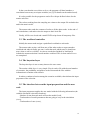
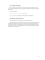
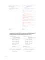
And finally here is the OUTPUT routine before and after the changes.
Here the parts that do not get commented out are in colour.
SUBROUTINE OUTPUT
1
(NCHAIN,NOUT,MXFL)
C-------------------------------------------------------------C
INCLUDE 'CPARAM.INC'
C
INCLUDE 'COTISP.INC'
INCLUDE 'CNUCNA.INC'
INCLUDE 'CNUCLI.INC'
INCLUDE 'CBIOSP.INC'
INCLUDE 'COUTPS.INC'
C
LOGICAL MXFL
C
NLY=MXNLYS
NELCHN=NEL(NCHAIN)
C
C.....write maximun flux at the
end of each one of the geosphere
C....layers for each nuclide and
time associated (if MXFL = 1 )
C
IF (MXFL) THEN
38
SUBROUTINE OUTPUT
1
(NCHAIN,NOUT,MXFL,fot3)
C---------------------------------------------------------------------C
INCLUDE 'CPARAM.INC'
C
INCLUDE 'COTISP.INC'
INCLUDE 'CNUCNA.INC'
INCLUDE 'CNUCLI.INC'
INCLUDE 'CBIOSP.INC'
INCLUDE 'COUTPS.INC'
C
LOGICAL MXFL
integer fot3
C
NLY=MXNLYS
NELCHN=NEL(NCHAIN)
C
C.....write maximum flux at the end
of each one of the geosphere
C.....layers for each nuclide and
time associated (if MXFL = 1 )
C
IF (MXFL) THEN
DO 10 LY = 1,NLY
WRITE(6,2000)
WRITE(6,2010)
DO 20 I = 1,NELCHN
DO 10 LY = 1,NLY
WRITE(6,2000)
WRITE(6,2010)
DO 20 I = 1,NELCHN
C
C
write(fot3,'(D13.7)') cmxx(i,ly)
WRITE(6,2020) LY,BNAME(NCHAIN,I),
CMXX(I,LY),TMXX(I,LY)
1
DOSEA(I)
20
10
…
IF (LY .EQ. NLY) THEN
WRITE(6,2030)
ENDIF
CONTINUE
CONTINUE
ENDIF
C
1
WRITE(6,2020) LY, BNAME(NCHAIN,I),
CMXX(I,LY),TMXX(I,LY)
IF (LY .EQ. NLY) THEN
WRITE(6,2030)DOSEA(I)
ENDIF
C
C
20
10
CONTINUE
CONTINUE
…
39
40
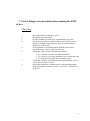
7. List of things to keep in mind when running the PMC
driver
Checklist:
1.
2.
3.
4.
5.
6.
7.
8.
Set total number of variables (ivar).
Set number of runs (iruns).
Set the variable sim to the type of simulations you want.
Set the correct values for the switches switch and sgenop for
single or multiple runs and for the type of random number
generator, respectively).
If the program is to load the matrix with the input values,
check check the value is right for sinfilemat.
Check the values for the correlation procedure:
• key activates or deactivates the correlation;
• var1 and var2, the user parameters to be correlated; and
• correlat should contain the correlation value.
Check the variables connected with the bayesian layer: sbayes,
nsche, distrifile and constfile.
Delete the temporary variables in the event that the program
stops abnormally (mcdname, mcdnr, mcdconst*, mcdtimeout*,
mcdout*).
41
42
Glossary
Bayesian Layer - Part of the PMC driver that selects the scenario to simulate. It
enables the uncertainty analysis to be made as described in reference [1].
Case - This is to enable a user to perform several MC simulations, each with a
different variable varying on its own. Each simulation is referred to as a case. At the
end, the PMC driver performs a simulation with all variables varying. The latter is
referred to as an additional case.
Distribution parameters - Usual values that characterise a particular probability
distribution: maximum, minimum, mean and standard deviation.
Input Preparator - Part of the PMC driver that samples the random values to
obtain the input values for the user model. It performs other tasks, like synchronising
all the nodes that are to work in parallel.
Macroscenario - A few general, distinct situations that are intrinsic to the study
of the model. See a practical implementation of this concept in [1].
Master node - the node, in a parallel machine, that is assigned the rank number 0
(zero). In our implementation, the root node is the node that runs the entire PMC
driver and takes care of spawning/collecting the input/output values for/from the rest
of the nodes involved in the calculation.
Message Passing Interface (MPI) - This is a library of standard subroutines for
sending and receiving messages and performing collective operations.
Microscenario - Within each macroscenario there should be a few scenarios that
still correspond to different situations. The microscenarios should be grouped under
each of the more general macroscenarios. On the other hand, each microscenario
should contain a detailed description of the situation, meaning that it should contain a
complete set of inputs for the user model. See [1] for a more detailed description of a
particular implementation.
Monte Carlo Simulation, see simulation.
43
Node - Component of a massive parallel machine consisting of a processor, a hard
disk and a local memory system (usually this is simply a workstation or equivalent
computer).
Parallel environment - System of computers that, through the use of an
appropriate software package, can work collectively on the solution of a numerical
problem.
Pseudo-random number generator - Set of numerical algorithms that generates
a stream of numbers that can perform the role of an ideal random stream of numbers.
Quasi-random number generator - Set of numerical algorithms that generates a
stream of numbers that are carefully selected to cover the space of input parameters
relevant to a particular model, in an efficient way.
Scenarios - Set of input values (for the user model) that describes a distinct real
situation that the user model is to simulate.
Simulation, Monte Carlo - Stochastic run of a user model with different input
values for its parameters in each run. The input values are usually sampled from
probability distributions that describe the probability of occurrence of each input
value. The number of runs should be high to obtain statistical significance (with the
use of parallel computers, one can easily attain hundreds of thousands of runs for a
simple user model). The usual output is another distribution built from the different
outputs generated during the runs.
Sobol indices – A particular algorithm that implement the concept of a quasirandom number generator.
User program - General denomination for the computer code that is to be
attached to the PMC driver. It would usually be a numerical implementation of a
mathematical model of a system.
User (model) parameters - The input parameters that the user program needs in
order to run.
44
References
[1] GESAMAC First Year Report, CIEMAT/IMA/550/55d18/38/96, December
1996 and references therein.
[2] Press, W., Flannery, B., Teukolsky, S., and Vetterling, W., Numerical Recipes,
Cambridge Press, 1986.
[3] Prado, P., User’s manual for the GTM-1 computer code, EUR 13925 EN,
ISSN 08-5593.
[4] Foster, I., Designing and building parallel programs, Addison Wesley, 1995.
[5] Sobol, I. M., Turchaninov, V. I., Levitan, Yu. L., and Shukman, B. V.,
Keldysh Inst. of Applied Mathematics, Russian Academy of Sciences, Quasirandom
Sequence Generators, Moscow, 1992, IPM Zak., No.30.
[6] Pereira, A., and Sundström, B., A Method to Induce Correlations between
Distributions of Input Variables for Monte Carlo Simulations. (submitted for
publication)
45