Download Cpipe User Guide

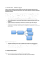
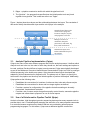
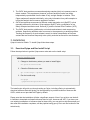
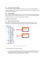
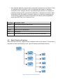
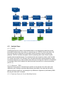
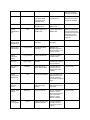
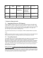
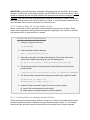
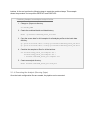
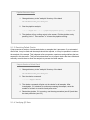
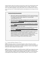
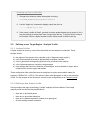
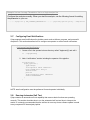
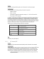
Cpipe User Guide
1. Introduction -­‐ What is Cpipe? ................................................................................................... 3 2. Design Background ...................................................................................................................... 3 2.1. Analysis Pipeline Implementation (Cpipe) ................................................................................ 4 2.2. Use of a Bioinformatics Pipeline Toolkit (Bpipe) .................................................................... 4 2.3. Individual Analysis Tools ................................................................................................................. 5 3. Installation ...................................................................................................................................... 6 3.1. Download Cpipe and Run Install Script ....................................................................................... 6 3.2. Create an Analysis Profile ................................................................................................................ 7 3.3. Create a Batch ....................................................................................................................................... 7 4. Directory Structure ...................................................................................................................... 7 4.1. Main Directory Structure ................................................................................................................. 7 4.2. Batch Directory Structure ................................................................................................................ 8 5. Reference Data ............................................................................................................................... 9 6. Software Process ........................................................................................................................ 10 6.1. Software Flow ..................................................................................................................................... 10 6.2. Analysis Steps ..................................................................................................................................... 11 6.2.1. FastQC ............................................................................................................................................................... 11 6.2.2. Alignment / BWA ......................................................................................................................................... 11 6.2.3. Duplicate Removal (Picard Markduplicates) ................................................................................... 11 6.2.4. GATK Local Realignment .......................................................................................................................... 12 6.2.5. GATK Base Quality Score Recalibration (BSQR) ............................................................................ 12 6.2.6. GATK Haplotype Caller .............................................................................................................................. 12 6.2.7. Filtering to Diagnostic Target Region ................................................................................................. 12 6.2.8. Variant Effect Predictor (VEP) Annotation ...................................................................................... 13 6.2.9. Annovar Annotation ................................................................................................................................... 13 6.2.10. Adding to Database .................................................................................................................................. 13 6.2.11. BEDTools / GATK Coverage ................................................................................................................. 13 6.2.12. Variant Summary ...................................................................................................................................... 13 6.3. Base Dependencies ........................................................................................................................... 14 6.4. Software List ....................................................................................................................................... 14 7. Resource Requirements .......................................................................................................... 16 7.1. Computational Resources (CPU, Memory) ............................................................................... 16 7.2. Storage Requirements ..................................................................................................................... 16 8. Gene Prioritisation .................................................................................................................... 17 9. Operating Procedures .............................................................................................................. 17 9.1. Performing an Analysis ................................................................................................................... 17 9.1.1. Prerequisites .................................................................................................................................................. 17 9.1.2. Creating a Batch for a Single Analysis Profile .................................................................................. 18 9.1.3. Creating a Batch for Multiple Analysis Profiles .............................................................................. 18 9.1.4. Executing the Analysis (Running Cpipe) ........................................................................................... 19 9.1.5. Resolving Failed Checks ............................................................................................................................ 20 9.1.6. Verifying QC Data ......................................................................................................................................... 20 9.2. Stopping an Analysis that is Running ......................................................................................... 22 9.3. Restarting an Analysis that was Stopped .................................................................................. 23 9.4. Diagnosing Reason for Analysis Failure .................................................................................... 23 9.5. Defining a new Target Region / Analysis Profile .................................................................... 24 9.5.1. Analysis Profiles ........................................................................................................................................... 24 9.5.2. Defining a New Analysis Profile ............................................................................................................ 24 9.6. Adjusting Filtering, Prioritization and QC Thresholds ......................................................... 25 9.6.1. Threshold Parameters ............................................................................................................................... 25 9.6.2. Modifying Parameters Globally ............................................................................................................. 26 9.6.3. Modifying Parameters for a Single Analysis Profile ..................................................................... 26 9.6.4. Modifying Parameters for a Single Analysis .................................................................................... 26 9.7. Configuring Email Notifications ................................................................................................... 27 9.8. Running Automated Self Test ........................................................................................................ 27 10. Cpipe Script Details ................................................................................................................ 28 10.1. QC Excel Report ............................................................................................................................... 28 10.1.1. QC Summary PDF ...................................................................................................................................... 29 10.1.2. Variant Summary Script: vcf_to_excel .............................................................................................. 30 10.1.3. Sample Provenance PDF Script ........................................................................................................... 30 11. Software Licensing .................................................................................................................. 32 12. Glossary ...................................................................................................................................... 32 1. Introduction - What is Cpipe?
Cpipe is a variant detection pipeline designed to process high throughput sequencing data
(sometimes called "next generation sequencing" data), with the purpose of identifying potentially
pathogenic mutations.
Software components are essential to every stage of modern sequencing. Cpipe covers only a
specific part of the process involved in producing a diagnostic result. The scope begins with a
set of short sequencing reads in FASTQ format. It ends with a number of outputs, as follows:
•
•
•
•
A set of identified variants (differences between the sample DNA and the human
reference genome) identified by their genomic position and DNA sequence change
A set of annotations for each mutation that describe a predicted biological context of the
mutations.
Quality measures that estimate the confidence in predictions about the mutations
Quality control information that allows accurate assessment of the success of the
sequencing run, including a detailed report of any regions not sequenced to a sufficiently
high standard
Mutations FASTQ Reads Software Pipeline (Cpipe) Annotations Quality Control Measures Cpipe does not currently cover:
•
•
Software processes that occur prior to sequencing, that are part of the sequencing
machines or steps after sequencing that are used to produce reads in FASTQ format.
Software that is used to view, manipulate, store or interpret mutations downstream from
the variant data is output by this process
2. Design Background
Cpipe uses an architecture that is comprised of three separate layers:
1. A set of core bioinformatics tools that are executed to perform the analysis
2. Bpipe - a pipeline construction toolkit with which the pipeline is built
3. The "pipeline" - the program that specifies how the bioinformatics tools are joined
together into a pipeline. This is what we refer to as "Cpipe".
Figure 1 depicts these three layers and the relationships between the layers. The remainder of
this section briefly describes each layer and the role it plays in the analysis.
Command Cpipe Specifies flow of data, order of execution of programs, locations of inputs, outputs, and programs to execute. Bpipe Manages execution of commands, keeps file provenance, audit trails, log files, sends notifications Command Command Individual analysis tools. Perform individual steps of the analysis. Figure 1 Layered architecture of the Cpipe Architecture
2.1. Analysis Pipeline Implementation (Cpipe)
Cpipe is the name of the main software program that runs the analysis process. It defines which
analysis tools are to be run, the order in which they should run, the exact settings and options to
be used, and how files should flow as inputs to each command. Cpipe was originally developed
as part of the Melbourne Genomics Health Alliance Demonstration Project, an effort to prototype
clinical sequencing in the health care system. Cpipe has since been further developed and
adapted by clinical laboratories for diagnostic use. The primary role of Cpipe is to specify the
tools used in the pipeline and how they are linked together to perform the analysis. Additionally,
Cpipe performs the following roles:
•
•
•
•
Establishes the conventions for locations of reference data, tools and software scripts
Establishes the conventions for where and how target regions are defined
Provides a system for configuration of the pipeline that allows settings to be easily
customised, versioned and controlled
Provides a set of custom scripts that perform quality control checks, summarize pipeline
outputs and collate data to prepare it for use in clinical reports
2.2. Use of a Bioinformatics Pipeline Toolkit (Bpipe)
Analysis of modern, high throughput genomic sequencing data requires many separate tools to
process data in turn. Coordinating and managing the execution of so many separate commands
in a controlled manner requires many features that are not provided by general purpose
programming languages. For this reason, Cpipe uses a dedicated pipeline construction
language called Bpipe[1]. Bpipe eases construction of analysis pipelines by automatically
providing features needed to ensure robustness and traceability. These features include:
1. Traceability
a. All commands executed are logged with all components fully resolved to
concrete files and executable commands
b. Versions of all tools used in processing every file are tracked and documented in
a database
c. All output from every command is captured in a log file that can be archived for
later inspection
2. Robustness
a. All commands are explicitly checked for successful execution so that a command
that fails is guaranteed to cause termination of processing of the sample and
reporting of an error to the operator
b. The outputs expected from a command are specified in advance, and Bpipe
verifies that expected outputs were successfully created
Bpipe is not further defined in this document. Extensive documentation is available online
[http://bpipe.org] and it is supported by a comprehensive test framework containing 164
regression tests that ensure critical features operate correctly.
2.3. Individual Analysis Tools
The core of the bioinformatics analysis applied by Cpipe is a set of tools that produce the
analytic result. The set of tools chosen are primarily based on the GATK [2] best practise
guidelines for analysis of exome sequencing data, which are published by the Broad Institute
(MA, USA). These guidelines are widely accepted as an industry standard for analysis of exome
data. However the guidelines are developed for use in a research setting, and thus are not
appropriate for use in clinical settings without modification. Cpipe therefore adapts the
guidelines to a) conform to necessary constraints and b) add required features, needed for use
in a clinical diagnostic setting.
The following are the key adaptations made to the GATK best practices:
1. The GATK best practice guidelines are designed to perform a whole exome analysis that
reports all variants found. Diagnostic use, however, is usually targeted to a particular
clinically relevant gene list. To enable this, the Cpipe allows specification of subset of
genes (the "diagnostic target region") to be analyzed on a per-sample basis. This
diagnostic target is combined with other settings that may be specific to the particular
target region to form an overall "Analysis Profile" that controls all the settings for a
particular analysis being conducted. Cpipe filters out all variants detected outside the
diagnostic target region from appearing in the results.
2. The GATK best practice guidelines do not include quality control steps. Cpipe adds
many quality control steps to the GATK best practices
3. The GATK best practices recommend analyzing samples jointly to increases power to
detect variants. This requirement, however, prevents analysis results from being
independently reproducible from the data of only a single sample in isolation. Thus
Cpipe analyses all samples individually, using only information from public samples to
inform the analysis about common population variants.
4. GATK best practices recommend a different variant annotation tool (SnpEFF) to that
generally preferred by clinicians. Cpipe replaces SnpEFF with a combination of two
widely accepted annotation tools: Annovar [3], and the Variant Effect Predictor (VEP).
5. The GATK best practice guidelines do not include mechanisms to track sequencing
artefacts. Sequencing artefacts arise from errors in the sequencing or analysis process.
Tracking the frequency of such variants is an aid to clinical interpretation as it allows
variants that are observed frequently to be quickly excluded as causal for rare diseases.
3. Installation
Cpipe is hosted at Github. To install Cpipe follow these steps.
3.1. Download Cpipe and Run Install Script
Follow the steps below to get the Cpipe source code and run the install script.
Steps for Installing Cpipe
1. Change to the directory where you want to install Cpipe:
cd /path/to/install/dir
2. Clone the Github source code:
git clone https://github.com/MelbourneGenomics/cpipe.git
3. Run the install script
cd cpipe
./pipeline/scripts/install.sh
The install script will guide you through setting up Cpipe, including offering to automatically
download reference data and giving you the opportunity to provide locations of Annovar and
GATK, which are not provided with Cpipe by default.
Please note that the installation will take a significant amount of time if you wish to use the built
in facilities to download and install reference data for hg19, Annovar and VEP. If you have your
own existing installations of reference data for these tools, you may wish to skip these steps and
then after the installation completes, edit the pipeline/config.groovy file to set the locations of the
tools directly.
3.2. Create an Analysis Profile
The next step after running the installation script will be to configure an analysis profile that
matches the target region for your exome capture and the genes you want to analyse. Proceed
by following steps in Section 9.5.
3.3. Create a Batch
Once you have defined an analysis profile you can then analyse some data using that analysis
profile. To do this, follow the steps outlined in Section 9.1.2. The process for creating the batch
will end with instructions for how to run the analysis for that batch.
4. Directory Structure
4.1. Main Directory Structure
Cpipe defines a standard directory structure that is critical to its operation (Figure 2). This
directory structure is designed to maximize the safety and utility of the pipeline operation.
Analysis data Analysis Profiles Figure 2 Directory structure d efined for Cpipe Two important features of this structure include:
•
For every batch of data that is processed, a dedicated directory holding all data related
to the batch is created. This reduces the risk that operations intended for a particular
batch of data will be accidently applied to the wrong batch.
•
Each separate diagnostic analysis that is performed is configured by an Analysis Profile.
The analysis profile is defined by a set of configuration files stored in a dedicated
subdirectory of the "designs" directory. By standardizing the definition of analyses into
predefined analysis profiles, potential misconfiguration of analyses is prevented. When
configuring a batch for analysis, an operator needs only to specify the analysis profile.
This profile then applies all required configuration and settings (such as appropriate
target region BED files) for the analysis to use.
Directory
Description / Notes
batches
sequencing data storage and analysis results
designs
configuration of different target regions
pipeline
pipeline script and configuration files
tools
third party tools
hg19
primary reference data (human genome reference sequence, associated files)
4.2. Batch Directory Structure
Within each batch directory, Cpipe defines a standard structure for an analysis. This structure is
designed to ensure reproducibility of runs. Figure 3 illustrates the standard structure.
Figure 3 Cpipe batch directory structure The first level of directories contains three entries:
•
•
•
design - all the configuration and target region BED files are copied to this directory with
the first run of the analysis. This is done to ensure reproducibility. It means that later on,
the whole analysis can be reproduced even if the source configuration for the analysis
profile has been updated, as all the design files are kept specific to each batch.
data - all the source data, ie: reads in FASTQ format. This data is kept separate from all
analysis outputs because it is the raw data for the analysis. It means that the whole
analysis can be deleted and re-run without any risk of affecting the source data
associated with the analysis.
analysis - all computational results of the analysis are stored in the analysis directory.
This directory has its own structure as detailed below. This directory is made separate
so that all output from a run of the pipeline can be easily deleted and re-run while being
sure not to disturb the design files or the source data.
Inside the analysis directory a set of directories representing outputs of the analysis are created.
These are:
•
•
•
•
•
fastqc - output from the FASTQC [4] tool. This is one of the first steps run in the analysis.
Keeping this directory separate makes it easy to check at the start of an analysis to
inspect the quality of data.
align - all the files associated with alignment are kept in this directory. This includes the
original BAM files containing the initial alignment as well as BAM files from intermediate
steps that are used to produce the final alignment
variants - all variant calls in VCF format are produced in this directory, as well as all
outputs associated with variant annotation (for example, Annovar outputs)
qc - this directory contains intermediate results relating to quality control information. If
problems are flagged by QC results, more detail can be found in the files in this directory
results - all the final results of the analysis appear in this directory. By copying only this
directory, all the key outputs from the pipeline can be captured in a single operation.
5. Reference Data
Many parts of the analysis depend on reference data files to operate. These files define well
established The following table describes the inputs that are used in the analysis process.
Input File
Source
Description
1
HG19 Reference
Sequence
ftp://[email protected]
/bundle
Human genome reference sequence
2
dbsnp_138.hg19.vcf
ftp://[email protected]
HG19 dbSNP VCF File, version 138, defines
known / population variants
/bundle
3
Mills_and_1000G_gol
d_standard.indels.hg1
9.vcf
ftp://[email protected]
/bundle
Defines common / known highly confident
indels.
4
Exon definition file
UCSC refGene database [url]
Defines the start and end of each exon
Additional reference data files are downloaded by the annotation tools used. Specifically, VEP
and Annovar. See pipeline/scripts/ download_annovar_db.sh for the full list of databases
downloaded for annotation by Annovar.
6. Software Process
This section describes the analysis process used to detect mutations in sequencing data in
detail.
6.1. Software Flow
The analysis process proceeds conceptually as a sequence of steps, starting with files of raw
reads. Figure 4 shows a linearized version of the steps through which the analysis processes
FASTQ files from a single sample to produce annotated mutations. In the physical realization of
these steps, certain steps may be executed in parallel and some steps may receive inputs from
others that are not adjacent in the diagram. For the purposes of explanation, however, this
section treats them as an equivalent series of sequential steps.
Sequencing
Data
Alignment
(BWA)
FastQC
Annovar
VEP
Variant
Summary
Annotated
Mutations
Picard
MarkDuplicates
Filter to
Diagnostic
Target
Add to
Database
GATK
Haplotype
Caller
QC
Summary
GATK Local
Realignment
GATK Base
Quality Score
Recalibration
BEDTools
Coverage
QC Excel
Report,
Gap Analysis
Provenance
PDF
Figure 4 Linearised Software Process 6.2. Analysis Steps
6.2.1. FastQC
FastQC[4] performs a number of automated checks on raw sequencing reads that provide
immediate feedback about the quality of a sequencing run. FASTQC scans each read in the
input data set prior to alignment and calculates metrics that detect common sequencing
problems. FASTQC includes automated criteria for detecting when each of these metrics
exceeds normal expected ranges. Two measures (Per base sequence content, and Per base
GC content) are known to fail routinely when using Nextera exome capture technology. Apart
from these measures, any other measure that receives a FAIL flag from FASTQC is considered
an automatic failure for the sample and requires manual intervention to continue processing
(see 9.1.5).
6.2.2. Alignment / BWA
Alignment is the process of determining the position in the genome from which each read
originated, and of finding an optimal match between the bases in the read and the human
genome reference sequence, accounting for any differences. Alignment is performed by BWA
[5] using the 'bwa mem' command.
6.2.3. Duplicate Removal (Picard Markduplicates)
Preparation of samples for sequencing usually requires increasing the quantity of DNA by use of
polymerase chain reactions (PCR). PCR creates identical copies of single DNA molecules. The
number of copies is often non-uniform between different molecules and thus can bias the
assessment of allele frequency of variants. To mitigate this, a common practise is to only
analyse data from unique molecules. The duplicate removal procedure removes all pairs of
reads with identical start and end positions so that downstream analysis is performed only on
unique molecules. This step also produces essential metrics that are reported in QC output by
downstream steps.
6.2.4. GATK Local Realignment
The initial alignment by BWA is performed for each read pair independently, and without any
knowledge of common variation observed in the population. A second alignment step examines
all the reads overlapping each genomic position in the target region and attempts to optimise
the alignment of all the reads to form a consensus among all the reads at the location. This
process accepts a set of "gold standard" variants (see Section 5) as inputs which guide the
alignment so that if a common population variant exists at the location the alignment will be
produced that is concordant with that variant.
6.2.5. GATK Base Quality Score Recalibration (BSQR)
Sequencing machines assign a confidence to every base call in each read produced. However it
is frequently observed that these quality scores do not accurately reflect the real rate of actual
base call errors. To ensure that downstream tools use accurate base call quality scores, the
GATK BQSR tool identifies base calls that are predicted to be errors with high confidence and
compares the observed quality scores with the empirical likelihood that base calls are erroneous.
This is used to then write out corrected base call quality scores that accurately reflect real error
probabilities.
6.2.6. GATK Haplotype Caller
The GATK Haplotype Caller is the main variant detection algorithm employed in the analysis. It
operates by examining aligned reads to identify possible haplotypes at each possible variant
location. It then uses a hidden Markov model to estimate the most likely sequence of haplotype
pairs that could be represented by the sequencing data. From these haplotypes and their
likelihoods, genotype likelihoods for each individual variant is computed and when the likelihood
exceeds a fixed threshold, the variant is written as output to a VCF file.
Note: variant calling is performed over the whole exome
target region, not just the diagnostic region. The
purpose of this is to allow internal database variant
tracking to observe variant frequencies across the whole
exome for all samples. This aids in ascertaining low
frequency population variants and sequencing artefacts.
6.2.7. Filtering to Diagnostic Target Region
The variants are called over the whole target region of the exome capture kit. However we wish
only to report variants that fall within the prescribed diagnostic target region. At this step,
variants are filtered prior to any annotation. This ensures that there cannot be incidental findings
from genes that were not intended for testing.
6.2.8. Variant Effect Predictor (VEP) Annotation
VEP is a tool produced by the Ensembl [6] organization. It reads the VCF file from
HaplotypeCaller and produces a functional prediction about the impact of each variant based on
the type of sequence change, the known biological context at the variant site, and from known
variation at the site in both humans and other species.
6.2.9. Annovar Annotation
Annovar is a variant annotation tool similar to VEP. It accepts a VCF file as input, and produces
a CSV file containing extensive information about the functional impact of each variant. Annovar
annotations are the primary annotations that drive the clinically interpretable output of the
analysis.
6.2.10.
Adding to Database
Cpipe maintains an internal database that tracks variants over time. This variant database is
purely used for internal tracking purposes. It tracks every variant that is processed through the
pipeline so that the count of each variant can be later added to the variant summary output.
Note: the variant database is the only part of the
analysis pipeline that carries state between analysis
runs. To ensure reproducibility, the analysis first adds
variants to the database but then afterwards makes a
dedicated copy of the database that is preserved to
ensure any future reanalysis can reproduce the same
result.
6.2.11.
BEDTools / GATK Coverage
The total number of reads (or coverage depth) overlapping each base position in the diagnostic
target region is a critical measure of the confidence with which the genotype has been tested.
To measure the coverage depth at every base position, two separate tools are run. The first is
BEDTools [7], and the second is GATK DepthOfCoverage. BEDTools produces per-base
coverage depth calculations that are consumed by downstream tools to produce the gap
analysis. GATK DepthOfCoverage is used to calculate high level coverage statistics such as
median and mean coverage and percentiles for coverage depth over the diagnostic coverage
region.
6.2.12.
Variant Summary
Clinical assessment of variants requires bringing together a complete context of information
regarding each variant. As no single step provides all the information required, a summary step
takes the Annovar annotation, the VEP annotation, and the variant database information and
merges all the results into a single spreadsheet for review. This step also produces the same
output in plain CSV format. The CSV format contains exactly the same information, but is
optimised for reading by downstream software, in particular, for input to the curation database.
6.3. Base Dependencies
The table below lists base dependencies that are required by other tools and are not used
directly. Base dependencies are listed separately because they are provided by the underlying
operating system and are not considered part of the pipeline software itself. Nonetheless, their
versions are documented to ensure complete reproducibility.
Software
CentOS
Java
Version
6.6
OpenJDK 1.7.0_55
Description / Notes
Base Linux software distribution that provides all basic Unix utilities
that are used to run the pipeline
Dependency for many other tools implemented in Java
Groovy
2.3.4
Dependency for other tools implemented in Groovy
Python
2.7.3
Dependency for many other tools implemented in Python
Perl
5.10.1
Dependency for many other tools implemented in Perl
6.4. Software List
The table below lists the bioinformatics software dependencies for Cpipe. These dependencies
directly affect results output by the bioinformatics analysis.
It is important to note that each software tool is run with options that affect its behavior. These
options are not specified in this section. These options are specified in the software pipeline
script, which maintained using a software change management tool (Git). An example script
representing the full execution of the software is supplied as an appendix to this document
(TBC).
Software
Version
Inputs
Outputs
Description /
Notes
create_batch
.sh
595f9ab
Gene definition BED
file, UCSC refGene
database
BED file containing all
exons for genes in
input file, potentially
with UTRs trimmed
In house script
FASTQC
v0.10.1
Sanger ASCII33
encoded FASTQ
Format
HTML and Text
summary of QC
results on raw reads
Output summary is
reviewed to ensure
that read quality is
sufficient and no other
failures or unusual
warnings are present
BWA
0.7.5a
Sanger ASCII33
encoded FASTQ
Format (same as
FASTQC step)
Sequence Alignment
in SAM format
Samtools
0.1.19
Sequence Alignment
in SAM format
Sorted Alignment in
BAM format
Picard
MarkDuplicat
es
1.65
Sorted Alignment in
BAM format
Filtered Alignment in
BAM format
GATK
Quality Score
Recalibration
3.2-2-gec30cee
Filtered BAM
alignment
Recalibrated BAM
alignment
GATK Local
Realignment
3.2-2-gec30cee
Recalibrated BAM
alignment
BAM file with
alignment adjusted
around common and
detected Indels
GATK
Haplotype
Caller
3.2-2-gec30cee
Realigned BAM file
VCF file containing
variants called
VCF file
CSV file with variants
and annotations
Annovar CSV file,
gene definition BED
Annovar CSV file
containing exonic
regions plus splice
variants
Recalibrated BAM file
Plot of distribution of
DNA fragment sizes,
text file containing
percentiles of fragment
sizes
Annovar
August 2013
add_splice_v
ariants
6a2b228f
Picard
CollectInsert
SizeMetrics
1.65
Variant Effect
Predictor
(VEP)
74
VCF file filtered to
diagnostic target
region
VCF file annotated
with annotations from
Ensemble
merge_annot
ations
96aa1f9cc
Annovar CSV file
Merges annotations
based on UCSC
knowngene database
with annotations
based on UCSC
RefSeq database
bedtools
coverageBed
v2.18.2
Realigned BAM, gene
definition BED file
Text file containing
coverage at each
location in genes of
interest
Performs main
alignment step using
'bwa mem' algorithm
Removes reads from
the alignment that are
determined to be exact
duplicates of other
reads already in the
alignment
In house script
In house script
R / custom
script
R 3.0.2
4899d433
Text file from
coverageBed
Plots and statistics
showing coverage
distribution and gaps
In house script
vcf_to_excel
dd139a28
Augmented Annovar
CSV files, VEP
annotated VCF files
Excel file containing
variants identified,
combined with
annotations and
quality indicators
In house script
qc_excel_rep
ort
37265a29
Merged annovar CSV
outputs, statistics from
R coverage analysis
Excel file containing
QC statistcs for review
In house script
7. Resource Requirements
7.1. Computational Resources (CPU, Memory)
Cpipe uses Bpipe's support to allow it to run in many different environments. By default it will
run an analysis on the same computer that Cpipe is launched on, using up to 32 cores. These
defaults can be changed by creating a "bpipe.config" file in the "pipeline" directory that specifies
how jobs should be run. For more information about configuring Bpipe in this regard, see
http://docs.bpipe.org/Guides/ResourceManagers.html
The minimum required memory to run an analysis is 16GB of available RAM and 4 processor
cores.
NOTE: If a particular analysis is urgent, the operator will interact with the cluster administrator to
reserve dedicated capacity for the analysis operator's jobs, allowing them to proceed.
7.2. Storage Requirements
The storage required to run an analysis depends greatly on the amount of raw sequencing data
that is input to the process. A typical sequencing run containing 12 exomes produces
approximately 120GB of raw data. In such a case, the analysis process produces intermediate
files that consume approximately 240GB of additional space and final output files consuming
180GB. The intermediate files are automatically removed and do not affect the interpretation or
reproducibility of the final results. However sufficient space must exist during the analysis to
allow these files to be created.
Based on the above, an operator should ensure that at least 540GB is available at the time a
new analysis is launched. Typically the full results of the analysis will be stored online for a short
period to facilitate any detailed followup that is required (for example, if quality control problems
are detected). Cleanup of intermediate resources means that approximately 300GB is required
for ongoing storage of the results after the analysis completes.
8. Gene Prioritisation
Cpipe offers a built in system to cause particular genes to be prioritised in an analysis. Genes
can be prioritised at two fundamentally different levels:
•
•
Per-sample - these are specified in the samples.txt file that is created for samples
entering the pipeline
Per-analysis profile - these are specified by creating a file called 'PROFILE_ID.genes.txt'
in the analysis profile directory (found in the "designs" directory of the Cpipe installation).
The "PROFILE_ID" should be replaced with the identifier for the analysis profile.
To specify gene priorities for an analysis profile, first create the analysis profile using the normal
procedure (see Section 9.5), and then create the genes file (named as
designs/PROFILE_ID/PROFILE_ID.genes.txt) with two columns, separated by tabs. The first
column should be the HGNC symbol for the gene to be prioritised and the second column
should be the priority to be assigned. Priority 1 is treated as the lowest priority and higher
priorities are treated as more important. An example of the format of a gene priority list is shown
below:
DMD
3
SRY
3
PRKAG2
1
WDR11
1
Please note that gene priority 0 is reserved for future use as specifying genes to be excluded
from analysis.
9. Operating Procedures
9.1. Performing an Analysis
This section explains the exact steps used to run the bioinformatics pipeline (Cpipe) to produce
variant calls.
9.1.1. Prerequisites
Before beginning, several pre-requisites should be ensured:
1.
2.
3.
4.
The FASTQ source data is available
An analysis profile is determined
A unique batch identifier has been assigned
Sufficient storage space is available (see Section 7.2)
IMPORTANT: in the following steps, examples will be shown that use "batch001" as the batch
identifier, CARDIAC101 as the analysis profile, and NEXTERA12 as the exome capture. These
should be replaced with the real batch identifier and analysis profile when the analysis is
executed. Also, the root of the Cpipe distribution is referred to as $CPIPE_HOME. This should
either be replaced with the real top level directory of Cpipe, or an environment variable with this
name could be define to allow commands to be executed as is.
9.1.2. Creating a Batch for a Single Analysis Profile
Before a new batch of data is processed, some initialization steps need to be taken. These
steps create configuration files that define the diagnostic target region, the location of the data
and the association of each data file to a sample.
Creating a Batch From Sequencing Data
1. Change to Cpipe root directory:
cd $CPIPE_HOME
2. Create the batch and data directory
mkdir -p batches/batch_001/data
3. Copy the source data to the batch data directory. The source data can be
copied from multiple sequencing runs into the data directory.
cp /path/to/source/data/*.fastq.gz batches/batch_001/data
4. Run the batch creation script, passing the batch identifier and the analysis
profile identifier:
./pipeline/scripts/create_batch.sh batch_001 CARDIAC101 NEXTERA12
5. The batch creation script should terminate successfully and create files called
batches/batch_001/samples.txt
batches/batch_001/target_regions.txt
6. Inspect the files mentioned in step (5) to ensure correct contents:
a). correct files are associated to each sample
b). target region and analysis profile is correctly specified
9.1.3. Creating a Batch for Multiple Analysis Profiles
Cpipe can analyse multiple analysis profiles in a single run. However the default batch creation
procedure assumes that all the samples belong to the same analysis profile. To use multiple
analysis profiles, the batch creation script should be run multiple times to create separate
batches. At the end, perform the following steps to create the combined steps. This example
shows the procedure for two profiles PROFILE1 and PROFILE2:
Combining Samples from Multiple Analysis Profiles
1. Change to Cpipe root directory:
cd $CPIPE_HOME
2. Create the combined batch and data directory
mkdir -p batches/combined_batch_001/data
3. Copy the source data for ALL samples for all analysis profiles to the batch data
directory.
cp /path/to/source1/data/*.fastq.gz batches/combined_batch_001/data
cp /path/to/source2/data/*.fastq.gz batches/combined_batch_001/data
4. Combine the samples.txt files for all the batches:
cat batches/temp_batch_001/samples.txt \
batches/temp_batch_002/samples.txt \
> batches/combined_batch_001/samples.txt
5. Create an analysis directory:
mkdir batches/combined_batch_001/analysis
9.1.4. Executing the Analysis (Running Cpipe)
Once the batch configuration files are created, the pipeline can be executed.
Pipeline Execution Steps
1. Change directory to the "analysis" directory of the batch
cd batches/batch_001/analysis
2. Start the pipeline analysis:
../../../bpipe run ../../../pipeline/pipeline.groovy ../samples.txt
3. The pipeline will run, writing output to the screen. Exit the pipeline run by
pressing "ctrl+c". Then answer "n" to leave the pipeline running.
9.1.5. Resolving Failed Checks
Cpipe executes a number of automated checks on samples that it processes. If an automated
check fails, it may be fatal and the sample should be rejected, or it may be possible to continue
the analysis of the sample. This judgment relies on operator experience and guidelines that are
separate to this document. This procedure describes how to inspect checks that have failed and
manually override them to allow the analysis to process the failed sample.
Steps to Resolve a Failed Check
1. Change directory to the "analysis" directory of the batch
cd batches/batch_001/analysis
2. Run the checks command:
../../../bpipe checks
3. The checks command will print out the checks for all samples. After
investigation, if it is desired to continue processing the sample, enter the
number of a check to override it and press enter.
4. Restart the pipeline. If it is running, use the stop procedure (see 9.2) and then
the start procedure (see 9.3)
9.1.6. Verifying QC Data
Cpipe produces a range of QC outputs at varying levels of detail. This section describes steps
to take to verify the overall quality of the sequencing output for a sample. The steps in this
section only address aggregate, overall, quality metrics. They do not address QC at the gene,
exon or sub-exon level, for which detailed inspection and judgement about each gene must be
made.
Verifying QC Output From an Analysis
1. Open the QC summary excel spreadsheet file. This file is named according to
the analysis profile and resides in the "results" directory ending with ".qc.xlsx".
For example, for analysis profile CARDIAC101 it would be called
"results/CARDIAC101.qc.xlsx"
2. Check that the mean and median coverage levels for each sample are above
expected thresholds. (NOTE: these thresholds are to be set experimentally
and are not defined in this document).
3. Check percentile of bases that achieve > 50x coverage is above the required
threshold (NOTE: this threshold is to be set experimentally and is not defined
in this document).
4. Open the insert size metrics file, found in
qc/<SAMPLE>.*.recal.insert_size_metrics.pdf where SAMPLE is the sample
identifier. Check that the observed insert size distribution matches
expectations. (NOTE: these expectations are to be set experimentally and is
not defined in this document).
5. Open the sample similarity report, found in qc/similarity_report.txt. Check for
unusual distribution of variants between samples. In particular, no two
samples should be much more similar than other samples. If this is the case,
further investigation should be carried out to rule out sample mixup,
unexpected relatedness, or sample contamination. The last line of the
similarity report will suggest any potentially related samples.
9.1.7. Analysing Related Samples (Trios)
NOTE: Family aware analysis is still under development in Cpipe. This section contains
preliminary information on how to perform trio analysis, however it should not be construed as
implying that Cpipe is fully optimised for trio analysis. In particular, it does not cause Cpipe to
perform joint variant calling on the related samples.
NOTE: The family-mode analysis uses SnpEff annotations. SnpEff is not configured for use by
the default installer. To use family-mode analysis, first configure SnpEff by creating the file
<cpipe>/tools/snpeff/3.1/snpEff.config and editing the data_dir variable. You may then need to
install appropriate SnpEff databases, using the SnpEff "download" command, for example:
java -Xmx2g -jar tools/snpeff/3.1/snpEff.jar download -c
tools/snpeff/3.1/snpEff.config hg19
In order to analyse related samples, Cpipe requires a file in PED format that defines the sexes,
phenotypes and relationships between the different samples. In the following it is assumed that
the PED file is called samples.ped. It should be placed alongside samples.txt in the analysis
directory for the sample batch to be analysed.
The current family analysis outputs a different format spreadsheet ending in ".family.xlsx". Inside
the family spreadsheet, instead of being a tab per sample, there is a tab-per-family. Each family
tab contains columns for each family member. The variants in the family spreadsheet are
filtered such that ONLY variants found in probands are present. Variants found only unaffected
family members are removed. The family member columns contain "dosage" values
representing the number of copies of the variant observed in each family member. That is, for a
homozygous mutation the number would be 2, while for a heterozygous mutation the number
would be 1, and if the variant was not observed in the sample the number is 0.
Running an Analysis in Family Mode
1. Change to the directory where the analysis is running
cd $CPIPE_HOME/batches/batch001/analysis
2. Run the pipeline, passing parameters to enable SnpEFF and family output:
../../../bpipe run \
-p enable_snpeff=true \
-p enable_family_excel=true \
../../../pipeline/pipeline.groovy \
../samples.txt ../samples.ped
9.2. Stopping an Analysis that is Running
An operator may desire to stop an analysis that is midway through execution. This procedure
allows the analysis to be stopped and restarted at a later time if desired.
Stopping a Running Analysis
1. Change to the directory where the analysis is running
cd $CPIPE_HOME/batches/batch001/analysis
2. Use the "bpipe stop" command to stop the analysis
../../../bpipe stop
3. Wait until commands are stopped
9.3. Restarting an Analysis that was Stopped
After stopping an analysis, it may be desired to restart the analysis again to continue from the
point where the previous analysis was stopped.
Restarting a Stopped Analysis
4. Change to the directory where the analysis is running
cd $CPIPE_HOME/batches/batch001/analysis
5. Use the "bpipe retry" command to restart the analysis
../../../bpipe retry
6. Wait until pipeline output shows in console, then press "Ctrl-C". If prompted to terminate
the pipeline from running, answer "n".
9.4. Diagnosing Reason for Analysis Failure
If an analysis does not succeed, the operator will need to investigate the cause of the failure.
This can be done by reviewing the log files associated with the run.
Reviewing Log Files for Failed Run
7. Change to the directory where the analysis is running
cd $CPIPE_HOME/batches/batch001/analysis
8. Use the "bpipe log" command to display output from the run
../../../bpipe log -n 1000
9. If the cause is visible in Step 2, proceed to resolve problem based on log output. If not, it
may be required to review more lines of output from the log. To do that, return to Step 2
but increase 1000 to a higher number until the failure cause is visible in the log.
9.5. Defining a new Target Region / Analysis Profile
9.5.1. Analysis Profiles
A Cpipe analysis is driven by a set of files that define how an analysis is conducted. These
settings include:
a)
b)
c)
d)
e)
the regions of the genome to be reported on (the "diagnostic target region")
a list of transcripts that should be preferentially annotated / reported
a list of genes and corresponding priorities to be prioritized in the analysis
a list of pharmacogenomic variants to be genotyped
other settings that control the behavior of the analysis, such as whether to report splice
mutations from a wider region than default.
These configuration files are defined as a set and given an upper case symbolic name (for
example, CARDIAC101, or EPIL). This symbol is then used throughout to refer to the entire set
of files. For the purpose of this document, we refer to this configuration as an "analysis profile".
9.5.2. Defining a New Analysis Profile
In this procedure the steps for defining a "simple" analysis profile are defined. The simple
analysis profile has the following simplifications:
•
•
•
•
there are no prioritized genes
there are no prioritized transcripts
there are no pharmacogenomic variants to be genotyped
all other settings remain at defaults
Defining a Simple Analysis Profile
Note: in these instructions, the analysis profile is referred to as MYPROFILE. This
should be replaced with the new, unique name for the analysis.
Note: in these instructions, the input target regions are referred to as
INPUT_REGIONS.bed. These are the regions that will be reported in results.
1. Run the target region creation script:
./pipeline/scripts/new_target_region.sh MYPROFILE INPUT_REGIONS.bed
2. Check the output:
head designs/MYPROFILE/MYPROFILE.bed
Verify: Correct genes and expected genomic intervals present at start of file
9.6. Adjusting Filtering, Prioritization and QC Thresholds
Cpipe uses a number of thresholds for filtering and prioritizing variants, and for determining
when samples have failed QC. These are set to reasonable defaults that were determined by
wide consultation with clinicians and variant curation specialists in the Melbourne Genomics
Health Alliance Demonstration Project. This section describes how to change these settings,
either globally for all analyses, for an analysis profile, or for a single analysis.
9.6.1. Threshold Parameters
This section documents some of the parameters that can be customized in Cpipe. Please note
that more parameters may be available, and can be found by reading the documentation found
in the pipeline/config.groovy file (or in pipeline/config.groovy.template).
Software
Default
Description / Notes
LOW_COVERAGE_THRESHOLD
15
The coverage depth below which a region is reported as
having "low coverage" in the QC gap report
LOW_COVERAGE_WIDTH
1
The number of contiguous base pairs that need to have
coverage depth less than the
LOW_COVERAGE_THRESHOLD for a region to be
reported in the QC gap report
MAF_THRESHOLD_RARE
0.01
The population frequency below which a variant can be
categorized as rare. The frequency must be below this
level in all databases configured (at time of writing, ExAC,
1000 Genomes and ESP6500).
MAF_THRESHOLD_VERY_RARE
0.0005
The population frequency below which a variant can be
categorized as very rare. The frequency must be below
this level in all databases configured (at time of writing,
ExAC, 1000 Genomes and ESP6500).
MIN_MEDIAN_INSERT_SIZE
70
The minimum median insert size allowed before a sample
is reported as failing QC
MAX_MEDIAN_INSERT_SIZE
240
The maximum median insert size allowed before a
sample is reported as failing QC
MAX_DUPLICATION_RATE
30
The maximum percentage of reads allowed as PCR
duplicates before a sample is reported as failing QC
CONDEL_THRESHOLD
0.7
The Condel score above which a variant may be
categorized as "conserved" for the purpose of selecting a
variant priority.
2
The distance in bp from end of exon from which a variant
is annotated as a splicing variant.
splice_region_window
9.6.2. Modifying Parameters Globally
To modify a configuration parameter globally for all analysis profiles, it should be set in the
pipeline/config.groovy file. Numeric parameters are simply set by assigning their values directly
as illustrated below.
Example: Set Low Coverage Threshold to 30x
Edit pipeline/config.groovy to add the following line at the end:
LOW_COVERAGE_THRESHOLD=30
9.6.3. Modifying Parameters for a Single Analysis Profile
If you wish to set a parameter for a particular analysis profile, set it in the "settings.txt" file for the
analysis profile. This file is found as designs/PROFILE/PROFILE.settings.txt, where PROFILE is
the id of the analysis profile you wish to set it for. The syntax is identical to that illustrated for
modifying a parameter globally in Section 9.6.2.
9.6.4. Modifying Parameters for a Single Analysis
A parameter value can be overridden on a one-off basis for a particular analysis. This is done by
setting the parameter when starting the analysis with the "Bpipe run" command.
Example: Set Low Coverage Threshold to 30x for a Single Analysis Run
Configure the analysis normally. When you start the analysis, use the following format for adding
the parameter to your run:
../../../bpipe run -p LOW_COVERAGE_THRESHOLD=30 ../../../pipeline/pipeline.groovy ../samples.txt
9.7. Configuring Email Notifications
Cpipe supports email notifications for pipeline events such as failures, progress, and successful
completion. This section describes how to configure an operator to receive email notifications.
Configuring Email Notifications
1. Create a file in the operator's home directory called ".bpipeconfig" and edit it
vi ~/.bpipeconfig
2. Add a "notifications" section including the operator of the pipeline:
notifications {
cpipe_operator {
type="smtp"
to="<operator email address>"
host="<SMTP mail relay>"
secure=false
port=25
from="<operator email address>"
events="FINISHED"
}
}
NOTE: email configuration must be performed for each operator individually.
9.8. Running Automated Self Test
Cpipe contains an automatic self test capability that ensures basic functions are operating
correctly. This section describes how to run the automated self test and how to interpret the
results. It is strongly recommended that the self test is run every time a software update is made
to any component of the analysis pipeline.
The self test performs the following steps:
1. Creates a new batch called "recall_precision_test"
2. Copies raw data for NA12878 chromosome 22 to the batch data directory
3. Configures the batch to analyse using a special profile (NEXTERA12CHR22) that
includes all genes from chromosome 22 within the Nextera 1.2 exome target region.
4. Runs the analysis to completion, creating results directory, final alignments (*.recal.bam)
and final VCFs (*.vep.vcf)
5. Verifies concordance with gold standard variants specified by the Genome In a Bottle
consortium for NA12878 are above 90%.
6. Creates a new batch called "mutation_detection_test"
7. Copies a set of specially created reads containing spiked in variants that correspond to a
range of pathogenic variants including splice site mutations at various positions relative
to exon boundaries, stop gain and stop loss mutations.
8. Verifies that all spiked in mutations are identified correctly in the output
Running Self Test
1. Run the selftest script
./pipeline/scripts/run_tests.sh
2. Check for any reported errors. Explicit failures will be printed to the screen.
10. Cpipe Script Details
Most steps in Cpipe are implemented by third party tools that are maintained externally.
However some steps are implemented by custom software that is maintained internally. This
section gives details of the custom internal software steps.
10.1. QC Excel Report
Purpose
Creates a detailed per-sample report measuring the quality of the sequencing output for
the sample, and a gap analysis detailing every region sequenced to insufficient
sequencing depth for the sample.
Inputs
•
GATK DepthOfCoverage sample_cumulative_coverage_proportions files (1 per
sample)
•
BEDTools coverage outputs (per base coverage information, 1 per sample)
•
Picard Metrics file (output by Picard MarkDuplicates, 1 per sample)
Outputs
Excel file containing detailed quality control information for each input sample
Implementation
For each sample, the following summary information is reported:
•
Median coverage
•
Mean coverage
•
Percentage of diagnostic region with coverage > 1x, 10x, 20x, 50x and 100x
•
Percentage of PCR duplicates
In addition, a gap analysis is created for each sample that specifies all regions below a
predefined coverage threshold (default 20x). The gap analysis is created by scanning
the diagnostic target region and identifying all contiguous stretches of bases that are
covered with less than the threshold number of reads. For each such stretch (or "block")
of low coverage bases, a row is written to the spreadsheet containing the gene, and the
maximum, minimum and median coverage depth for bases inside the block.
Additionally, the following summary statistics are calculated:
Total low regions Total low bp Frac low bp Genes containing low bp Frac Genes containing low bp total number of contiguous regions where coverage depth is below threshold total number of base pairs where the coverage depth is below the threshold Fraction of base pairs where coverage depth is below threshold Total number of genes containing at least 1bp that is below threshold Fraction of genes containing at least 1bp that is below threshold File
scripts/qc_excel_report.groovy
10.1.1.
QC Summary PDF
Purpose
Creates a PDF that summarizes essential quality control information for the sample.
Implementation
The QC PDF script reads per-base coverage information that is calculated by BEDTools.
The script accepts an acceptable coverage threshold as input. For each gene in the
target region it calculates the percentage of base pairs that have read coverage depth
greater than the configured threshold. The script then creates a PDF file containing:
1. a table of genes showing the percentage of bases within each gene above the
acceptable threshold
2. a summary of overall coverage statistics for the sample
File
scripts/qc_pdf.groovy
10.1.2.
Variant Summary Script: vcf_to_excel
Purpose
Summarizes identified mutations and annotations from different tools into a single excel
spreadsheet
Inputs
•
VEP-annotated VCF file per sample
•
Enhanced Annovar annotation summary (CSV) per sample
•
Internal variant database (SQLite format)
Outputs
•
Excel spreadsheet summarizing variants identified for patient
•
CSV file for import to curation database
Implementation
The script reads in VEP-annotated VCF files and Annovar summary annotation files for
each sample in the cohort. For each Annovar annotation the equivalent variant is
retrieved from the sample VCF file. The script then writes a row into the spreadsheet
containing:
•
Annovar variant annotations
•
Priority index for variant
•
Gene category for variant
•
Count of number of observations of variant in internal database
In addition to writing each row to the Excel spreadsheet, the output is also written in CSV
format. The CSV format output is intended to be read by a database import script.
10.1.3.
Sample Provenance PDF Script
Purpose
To ensure reproducibility of processing by documenting the details of the input and
output files and the versions of software tools applied to them.
Implementation
The provenance script is implemented as an Bpipe report template, found in
pipeline/scripts/provenance_report.groovy. Bpipe report templates are scripts that have
full access to the pipeline meta data including all input and output files, their properties
and dependencies. The provenance report documents:
•
the time and date of the beginning and end of processing the sample
•
the patient identifier
•
the timestamps and file sizes of
•
o
the input FASTQ files
o
the initial alignment file (BAM file)
o
the final alignment file (ending in .recal.bam)
o
the raw VCF file
o
the annotation file produced by Annovar (CSV format)
o
the final Excel report containing variant calls
The version numbers of all the critical software components used in generating
the results
11. Software Licensing
This section details the licenses of software components used in Cpipe. This section is provided
for informational purposes only, and it is the responsibility of the user to check and agree to
actual license terms according to their own circumstances.
Software
License / Notes
Open Source
Bedtools
GPLv2
Samtools
MIT
Bpipe
BSD
BWA
GPLv3
Groovy
Apache 2.0
FastQC
GPLv3
VEP
Apache (modified – see http://www.ensembl.org/info/about/code_licence.html)
SQLite
Public Domain
Picard Tools
MIT
Groovy-ngs-utils
LGPL
excel-category
LGPL
IGVTools
LGPL
IGV
LGPL
VEP Condel Plugin
Apache (modified – see http://www.ensembl.org/info/about/code_licence.html)
Proprietary
GATK
Academic only, non-academic, commercial license
Annovar
Academic only, non-academic commercial license
12. Glossary
Term
Meaning
Exome target region
The genomic regions targeted by the exome capture kit
Diagnostic target region
The genomic region from which fully annotated variants will be included for
curation
Batch
A set of samples that are analysed together. Often (but not necessarily) a
complete set of data output by a single run of a sequencing machine.
Sequencing Run
The sequencing of a set of samples on a sequencing machine.
Batch identifier
A unique name that is used to track analysis of a particular set of data
Analysis profile
A diagnostic target region combined with predefined settings for running the
analysis pipeline that are appropriate for that diagnostic application
Annotation
Information about a variant that informs clinical interpretation. Examples include:
effect on protein sequence, population frequencies, predicted pathogenicity,
number of samples observed to carry the mutation
Priority index
An integer index assigned to a variant to indicate the severity of functional impact
on a protein it causes
Operator
A person who is controlling an analysis of a sequencing run
Gene category
An integer index assigned to a gene to indicate the strength of evidence of its
association to a particular disease. Can be specified per-patient for each gene.