Download Programita - Thorsten Wiegand

Extending Point Pattern Analysis for
Objects of Finite Size and Irregular Shape
using the Programita software
A supplementary user manual
with an collection of examples using the Programita software
Draft version
27 of July 2006
written by
Thorsten Wiegand
Department of Ecological Modelling,
UFZ-Centre for Environmental Research,
PF 500136,
04301 Leipzig, Germany,
Tel.: (**49) 341-235 2479
Fax: (**49) 341-235 3500
email: thorsten.wiegand@ ufz.de
2
SUPPLEMENTARY USER MANUAL FOR PROGRAMITA
THORSTEN WIEGAND
3
Contents
Programita.............................................................................................................5
Abstract ..............................................................................................................5
Before starting Programita ................................................................................5
Hardware requirements ..................................................................................5
Terms of use and copyright agreement ..........................................................6
Installation......................................................................................................6
Screen size......................................................................................................7
A quick start .......................................................................................................8
Execute Programita .......................................................................................8
Load a settings file to redo an analysis ..........................................................8
What happens on the screen? .........................................................................9
Show results of previous analyses ...............................................................10
Save the results of the analysis ....................................................................11
Temporary data-files ....................................................................................12
The input data files (*.dat and *.asc data files)................................................14
Preparation of data under matrix-mode .......................................................15
Format of the *.dat matrix data file..............................................................16
The Settings Menu for Point Pattern Analysis.................................................17
Matrix data ...................................................................................................17
Irregularly shaped study region....................................................................18
Irregularly shaped study region for matrix data...........................................18
Maximum scales r and ring width dr ...........................................................18
Background of second-order statistics .............................................................19
Second order statistics......................................................................................19
Definition of the bivariate K- and L-functions.............................................19
Definition of the g-function and of the O-ring statistic ...............................20
Grid-based estimators of second-order statistics .............................................21
Grid-based estimator of K- and L-function ..................................................21
Grid-based estimator of g- and O-function ..................................................22
Selection of ring width.................................................................................22
Considering finite size and irregular shape.....................................................23
Randomization of objects finite size and real shape ........................................24
Overlap between plants................................................................................25
Construction of objects from categorical map .............................................27
Separation of joined objects.........................................................................28
Manual separation of joined objects ............................................................28
Randomization of the position of objects ....................................................30
Edge correction if objects fall partly outside the study rectangle................31
Test of possible bias through edge correction..............................................32
Masking (space limitation)...........................................................................33
Circle approximation....................................................................................34
Point approximation .....................................................................................34
Null models for objects with finite size and irregular shape..........................35
CSR: Randomising plant position for univariate patterns ...............................35
4
SUPPLEMENTARY USER MANUAL FOR PROGRAMITA
CSR and rectangular study region (Example F_CSR_1.res)....................... 35
CSR in irregularly shaped study region with mask (Example F_CSR_2.res)39
Heterogeneous Poisson null model (HP)......................................................... 41
Heterogeneous Poisson (Example F_HP_1.res) .......................................... 43
Heterogeneous Poisson null model: plug-in intensity functions (Example
F_HP_2.res) ..................................................................................................... 46
Toroidal shift: Independence of bivariate patterns .......................................... 48
Toroidal shift (Example F_In_1.res) ........................................................... 48
Antecedent condition: Randomising only pattern 2 ........................................ 50
Antecedent condition (Example F_Ant_1.res) ............................................ 51
Antecedent condition (Example F_Ant_2.res) ............................................ 53
Antecedent condition (Example F_Ant_3.res) ............................................ 54
Antecedent condition (Example F_Ant_4.res) ............................................ 56
Random labelling............................................................................................. 57
Random labeling (Example RL_1.res) ........................................................ 58
References........................................................................................................... 61
THORSTEN WIEGAND
5
Programita
Abstract
The Programita software allows you to perform univariate and bivariate pointpattern analysis with Ripley's L-function, the pair-correlation function, and the
O-ring statistic. Programita contains standard and non-standard procedures for
most practical applications. Procedures for non-standard situations include the
possibility to perform point-pattern analyses for arbitrarily shaped study regions
and Programita offers a wide range of non-standard null models such as heterogeneous Poisson null models or cluster null models.
The grid-based implementation of Programita allows for a straight-forward extension of point pattern analysis to deal with objects of finite size and irregular
shape (e.g., plants). The objects are approximated by using the underlying grid
and may occupy several adjacent grid cells depending on their size and shape.
Null models correspond to that of point pattern analysis but need to be modified
to account for the finite size and irregular shape of plants.
The procedures used by Programita for performing analyses which consider the
finite size and irregular shape of objects are described in detail in Wiegand et al.
2006. This document supplements the manual of Programita, focusing on analyses of objects with finite size and irregular shape.
Before starting Programita
Hardware requirements
Programita is a free unsupported software, developed in Borland Delphi4 under
a WindowsXP environment. Programita is executable under 32-bit operating
systems such as Windows98, Windows 2000, Windows XP or WindowsNT.
Running Programita requires little hard drive space. For example, for grid sizes
< 200 ×200 cells Programita and temporally created files occupy < 10M. However, analysis of larger grid sizes may be slow for small working memory and
low computer speed.
6
SUPPLEMENTARY USER MANUAL FOR PROGRAMITA
Terms of use and copyright agreement
The Programita software is produced by Thorsten Wiegand in his spare time. He
is affiliated at the Dept. Ecological Modelling, UFZ Centre for Environmental
Research Leipzig-Halle. Programita is intended to foster analysis of point patterns in ecology by providing ecologists a tool that contains null models and procedures not supported by most statistical packages, but which are essential for a
throughout analysis of point-patterns. The Programita software is not a commercial venture and may be downloaded and used free of charge for purposes of
scientific research and teaching. Any commercial application of the program
requires the previous permission by the author. Publications must acknowledge
use of the Programita and cite Wiegand and Moloney (2004) which describes
the basic implementation and the procedures used by Programita and Wiegand
et al. (2006) for analyses of finite size and irregular shape.
Installation
There is no setup procedure; installation of Programita requires only the extraction of all files from the zip file Progamita_FiniteSize.zip. Make sure that you
also access the PDF (Manual_FiniteSize_Programita2006.pdf) and HTM versions (Manual_FiniteSize_Programita2006.zip) of the supplement user manual.
Place the files into a directory of your choice; extracting the zip file will place all
files into the sub-directory Programita. Note that you must place all files in the
same directory; for simplicity Programita does not use a path variable. The zipfile contains the following files and file types:
ProgramitaJulio2006.exe
*.asc files
*.dat files
*.int files
*.rep files
*.res files
the executable of Programita, version 26 of July
2006
example data file in ArcView raster format
example data files and temporary files
plug-in files for heterogeneous Poisson
data files to show results of previous analyses
results and settings files
The manual of Programita (Manual_FiniteSize_Programita2006.pdf) and a
HTM version of the manual (Manual_FiniteSize_Programita2006.zip) are provided separately. You can use the HTM version as help because it contains
many textmarks and internal links for easy navigation through the document.
THORSTEN WIEGAND
7
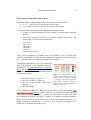
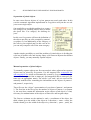
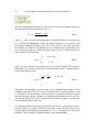
Screen size
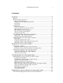
Programita was designed for a screen of 1024 × 768 pixels, but it can be run as
well using an 800 × 600 screen. If you execute Programita in the 1024 × 768
pixel mode, it must look like the segment shown in figure 1. Sometimes windows within Programita are truncated and one cannot see all of some buttons or
headers. In this case, it is as if the window is too small to handle them. To avoid
this problem, check the default letter size in the settings of your computer. Your
computer may scale the letters but not the window sizes and as a consequence,
the windows appear too small.
Figure 1. Correct display of the Programita interface under the 1024 × 768 pixel mode.
8
SUPPLEMENTARY USER MANUAL FOR PROGRAMITA
A quick start
Execute Programita
Execute and adjust Programita to your screen size. Two options
are given, a screen of 800 × 600 pixels, and a larger screen of
1024 × 768 pixels which is the default.
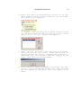
Load a settings file to redo an analysis
There is a convenient way to quickly start with
Programita and to learn the settings. You can read
a file (a *.res-file) that contains all setting of a previous analysis and redo this analysis. For example,
you can repeat all analysis show in the figures 2A C in Wiegand et al. (2006).
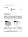
Figure 2. Load an example
settings file.
To load a settings-file, apply the button “Load Settings for Example” (figure 2)
and a list with files containing settings of old analysis will appear (figure 2).
Select a *.res-file, for example fig2A.res, press ”ok”, and then the button
“Calculate Index”. Now Programita performs the analysis of figure 2A in
Wiegand et al. (2006).
THORSTEN WIEGAND
9
What happens on the screen?
After loading the settings-file fig2A.res, Programita will automatically select
all settings for the data and analysis mode and all settings for the null model that
was used in the example fig2A.res.
Two plots will appear: on the left appears a plot showing the original point pattern being analyzed (figure 3a), and on the right appear the patterns of the
Monte Carlo simulations of the null model used for constructing the confidence
limits. After terminating the simulations of the null model, the figure with the
simulated patterns of the null model disappears, and instead a figure with the
result of the analysis appears on the right (figure 3b).
Figure 3a. Left: the point-pattern analyzed in
fig2A in Wiegand et al. (2006). Right: One
realization of the Monte Carlo null model that
conserves the shape of the shrubs (a random
pattern, CSR) used to construct the confidence
limits.
Figure3b. After termination of the
Monte Carlo simulations of the null
model, a figure with the result appears on the right. The figure shows
Wiegand-Moloney's O-ring statistic
(or Ripley's L-function) together
with the confidence limits for the
specific null model chosen. The top
figure shows the results of the univariate point pattern analysis; the
bottom figure shows the results of
the bivariate analysis if a second type
of points was specified. In fig2A
only one type of points was used.
Therefore, there appears no result for
the bivariate analysis.
10
SUPPLEMENTARY USER MANUAL FOR PROGRAMITA
Show results of previous analyses
Programita offers a convenient possibility to show the
results of previous analyses. (This works only if the
option “Combine replicates” was enabled when doing
the original analysis.)
To show the results of a previous analysis, apply the
button “Replicates” (figure 2) and a window with a list
of results files appears (figure 4). Highlight fig.2A.rep,
press “select file”, and “Calculate joined statistic”. The
result of the analysis will appear (figure 5).
Figure 4. A list with result files which were
previously saved.
Figure 5. The results of the previous analysis
fig2A.rep.
THORSTEN WIEGAND
11
Save the results of the analysis
To save the results of the analysis, press the button “save results” that appears
below the graph with the results of the univariate analysis (figure 3b), and insert
a name for the result file. The results file will be saved as ASCII-file name.res in
the same directory where the *.exe file of Programita is located. The results file
(figure 6) contains the settings of this analysis and the results of the univariate
and the bivariate point-pattern analysis. The results file name.res can be used (in
the same way as fig2A.res) in the previous section to load the setting and to repeat the analysis.
Pointpattern analysis of file D:\Programita\Figure2.asc
Method Wiegand-Moloney (ring) with 99 replicates for confidence limits, ring width = 3
Test Model= 12random 1shape
*
400
400 8 smaller
4
** 8
the null assumed homogeneous pattern(s)
Analysis modus= standard
only one point per cell allowed
All cells within the rectangle were considered for calculating the indices
number cells of pattern 1 = 1015
number cells of pattern 2 =
0
the rectangular area contains 130*274 = 35620
cells (= dim1*dim2)
pattern 1 was coded with numbers 11 * 11 * 11 * 11
pattern 2 was coded with numbers 2 * 2 * 2 * 2
the mask was coded with numbers -1 -1 -1
Scale
1
2
3
4
5
6
7
8
9
10
r
r
r
r
r
r
r
r
r
r
r
r
r
r
r
r
r
r
r
r
r
r
O11(r),
0.3999665
0.3003174
0.1851738
0.0968253
0.0579106
0.0391140
0.0329553
0.0361094
0.0425961
0.0484125
E11-,
0.3856460
0.2881745
0.1748624
0.0864759
0.0485426
0.0313220
0.0220457
0.0185628
0.0186002
0.0196974
E11+,
0.4191957
0.3228708
0.2109540
0.1244389
0.0833683
0.0652772
0.0598031
0.0582927
0.0557966
0.0514856
O12(r),
0.0000000
0.0000000
0.0000000
0.0000000
0.0000000
0.0000000
0.0000000
0.0000000
0.0000000
0.0000000
E12-,
0.0000000
0.0000000
0.0000000
0.0000000
0.0000000
0.0000000
0.0000000
0.0000000
0.0000000
0.0000000
E12+,
0.0000000
0.0000000
0.0000000
0.0000000
0.0000000
0.0000000
0.0000000
0.0000000
0.0000000
0.0000000
Figure 6. The *.res results file (fig2A.res). The first lines contain the information on the settings of the analysis; the following part contains a table with the results of the analysis. The first
column gives the spatial scale r of the point-pattern analysis units of cells, the second and third
column provide a summary of the Monte Carlo significance test of the null model ("-": data at
scale r below the confidence limits, "r": inside the confidence limits, and "+": above the confidence limits; second column for univariate analysis, third column for bivariate analysis), columns 4, 5, 6: results of univariate analysis (column 4: univariate O-statistic [or L-function] of
the data, column 5: lower confidence limit, column 6: upper confidence limit), and columns 7,
8, 9: results of bivariate analysis (column 7: univariate O-statistic or [or L-function] of the data,
column 8: lower confidence limit, column 9: upper confidence limit).
12
SUPPLEMENTARY USER MANUAL FOR PROGRAMITA
Temporary data-files
During the analysis, Programita creates a number of temporary data files which
are overwritten by a new analysis. Knowing these files, you may use the
information they contain.
The files tempp1.dat and tempp2.dat.⎯The file tempp1.dat contains a matrix
representation of pattern 1. The first line contains information on the dimensions of the grid: (1, number of lines, 1, number of columns). The following
lines are the data matrix with the pattern. The numbers are not code numbers as
in the matrix data format but give a “1” if the cell is occupied by category of
pattern 1 and a “0” if the cell is not occupied by the category of pattern 1. The
file tempp1.dat does not contain information on an irregularly shaped study region. The file tempp2.dat is the analogue to tempp1.dat for pattern 2.
The file temphab.dat.⎯If you analyze an irregularly shaped study region,
Programita creates a matrix representation of your study region analogously to
the files tempp1.dat and tempp2.dat.
The file tempp12.dat.⎯The file tempp12.dat is the “list in grid” representation of your data, containing the information on cells of pattern 1, pattern 2, and
the study region.
The files Bi_confidence.env and Uni_confidence.env.⎯Programita uses the
lowest and highest O(r) [or L(r)] of the different simulations of the null model
as default confidence limits. However, it automatically produces two temporally
files (Uni_confidence.env, Bi_confidence.env) that contain the O(r) [or L(r)] for
all simulations of the null model. The columns of these files are the scales r = 1,
rmax, and the lines are the different simulations of the null model. You may use
this information to construct confidence limits with different definitions. Note
that Programita offers the possibility to use also the 5th highest and 5th lowest
O(r) [or L(r)] out of 99 (or 999) replicate simulations of the null model for defining 95% (99%) confidence limits (e.g., Stoyan and Stoyan 1994).
The individual O and λK-function.⎯The individual O(r) of a cell (x, y) of
pattern 1 gives the density of pattern 1 cells in a ring with radius r around the
focal cell (x, y). The individual λK(r) of a cell (x, y) of pattern 1 gives the number of pattern 1 cells in a circle with radius r around the focal cell (x, y).
THORSTEN WIEGAND
13
The file temp_indO.dat gives the individual O(r) or λK(r) for each point of the
pattern. The file is comma-delimited and the first two columns give the x- and
y-coordinates of the cell of pattern 1. The next columns give the individual univariate O11(r) or λK11(r) [= O11(r) or K11(r)] for the cell (x, y) at scale r, and
the individual bivariate O12(r) or λK 12 (r) [=O12(r) or K12(r)]] for the cell (x, y)
at scale r. The end of the file gives the settings file (figure 5) used to generate
the data.
The files temppatch1.dat and temppatch2.dat.⎯These files are the “object”
representation of your data of pattern 1 and pattern 2. The first line gives the
number of objects of pattern 1 (or pattern 2), the next lines contain the information on the objects necessary for randomization of the objects of finite size and
irregular shape.
The first two columns are the minimal x- and y- coordinates of the object, the
third column gives the width of the object in x-direction (= xmax-xmin), the
fourth column gives the width of the object in y-direction (= ymax-ymin), the
fifth column the number of cells of the objects, and the following columns give
the pairs of coordinates belonging to the object.
For example, the beginning of the temppatch1.dat is given by:
126
1
185
2
2
6
1
186
1
187
2
186
2
187
2
185
3
186
and indicates that there are a total of 126 objects, and the minimal x- and ycoordinates of the first object are 1 and 185, respectively. The width in x- and ydirection of the object is 2 cells (xmax= 3, xmin=1; ymax=187, ymin = 185),
and the object comprises the six cells (1, 186), (1, 187), (2, 186), (2, 187), (2,
185), and (3, 186).
14
SUPPLEMENTARY USER MANUAL FOR PROGRAMITA
The input data files (*.dat and *.asc data files)
Programita performs point-pattern analysis for two different situations. First, it
calculates the O-ring statistic and the L-function for point patterns which are
basically given as a list of points with and without a predefined grid. This corresponds to conventional point-pattern analysis.
In a second mode, Programita performs point-pattern analysis for categorical
maps which can represent objects of finite size and irregular shape. In this case,
the data input is a matrix with categories that can range from 0 to 999. In the
following, we discuss the data input for categorical maps.
Because Programita works in the matrix mode
with a category and not with number of points,
the Monte Carlo simulation of null models differs slightly from the point mode. Under the
mode "Matrix" the null model does not allow to
have the same category two times in a given
cell. However, if you enable the checkbox
"Only one point per pattern" in the null-model
window (figure 7), Programita allows having a
mixed category where type 1 and type 2 are
together in one cell.
Figure 7. The null-model window
for the mode "Matrix".
THORSTEN WIEGAND
15
Preparation of data under matrix-mode
The input data are a matrix that can have the following code numbers:
• 0, 1, 2, ..., 999 if the cell is inside the study region
• -1 (or -9999) if the cell is outside the study region (mask)
Programita reads two different data formats in the matrix-mode:
1. a space (or tab) delimited ASCII-file with the *.dat extension with line
breaks.
2. the ASCII format of ArcView (a *.asc-file) without line breaks. The
head of the *.asc-file must look like this:
ncols 144
nrows 45
xllcorner 1
yllcorner 1
cellsize 1
nodata_value -9999
ncols gives the number of columns, nrows the number of rows, xllcorner the
smallest x-coordinate, and yllcorner the smallest y-coordinate. The cell size must
be "1" and the value for no data (the mask) must be -9999.
The matrix mode allows you to use a data matrix with different code numbers, however,
calculation of Wiegand-Moloney's O-ring statistic and Ripley's L-function Programita requires a reduction of the original code numbers
to the four categories:
Figure 8. Transformation of the
•
•
•
•
original code numbers of the data
matrix to the three categories: pattern
the cell is of type 1 (pattern 1)
1, pattern 2, and mask outside the
the cell is of type 2 (pattern 2)
study region. All other categories
the cell is outside the study region which are not set are automatically
(mask)
defined as empty cells.
the cell is empty
If you enable the "Matrix" or "Data are given as matrix" option, the window Give
code number for patterns (figure 8) appears and ask you to group your code numbers
into the final categories "pattern 1", "pattern 2", and "mask". All other cells with
code numbers not defines as pattern 1, pattern 2, or mask are defined automatically as empty cells. You can combine up to four code numbers (but not -1) to
define "pattern 1" and "pattern 2", and up to four categories (including -1) to
define the area outside the study region.
16
SUPPLEMENTARY USER MANUAL FOR PROGRAMITA
Thus, you can mask, if required, additionally cells which are part of the original
study region. For example, if you study vegetation maps with category 0: bare
ground, category 1: grass tufts (size of one cell) and category 2: shrubs (size of
several cells) you may mask the area occupied by shrubs for studying the spatial
pattern of the grass tufts. If you do not exclude the area occupied by shrubs
(which cover perhaps 10% or so of the study region) a simple null model that
randomizes the locations of the grass tufts (CSR) will distribute tufts at locations
where they cannot occur in the field. This may introduce a bias in the analysis.
The possibility to use up to 1000 categories is a convenient feature because you
can use the same data for different analyses. Be sure that a given code number
does not appear in different categories. A given cell can either be pattern 1, pattern 2, empty, or mask!
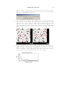
Format of the *.dat matrix data file
The *.dat matrix data-file is a space (or tab) delimited ASCII-file. The first line
contains information on the dimensions of the grid: (1, number of lines, 1, number of columns). The following lines are the data matrix with the different code
numbers. In contrast to the ArcView ASCII matrix format, you need to insert
line breaks. Note that the visualization of Programita corresponds to the transposed matrix. (figure 9).
Figure 9. Example of a *.dat input data-file for the matrix mode. Shown are the file
small_matrix.dat (left) and the visualization in Programita (right). Red: cells of pattern 1 (code
1), green: cells of pattern 2 (code 2), grey: empty cells (code 0), black: mask with cells outside
the study region (code -1). The first line contains information on the grid: (1, number of lines, 1,
number of columns). Note that the visualization of Programita corresponds to the transposed
matrix.
THORSTEN WIEGAND
17
The Settings Menu for Point Pattern Analysis
If you select in the menu What do you want to do?
"Point-pattern analysis", Programita allows you to
select different types of analysis, input data, input
data formats, etc. If you do not use a *.res settingsfile that stores the settings from a previous analysis
you need to carefully select all settings manually
from the settings menu before performing any analysis.
Programita calculates Ripley's L function (“Circle”
in Which method will you use) and Wiegand-Moloney's
O-ring statistic (“Ring” in Which method will you use) in
a grid-based implementation for a given data-file
(selected in Input data file).
In the window How are your data organized? you can
select between two types of input data: (1) data
which are given as a list of points and (2) categorical
data which are organized as a matrix.
Matrix data
If your data are a matrix (categorical data), you need
to select “Matrix” in How are your data organized?, “Data
are given as matrix map” in Select modus of data, and
specify in the window Give code numbers for pattern
which code numbers of your data matrix make up
pattern 1, pattern 2, and the mask. The mask defines
the area outside the study region if your study region
is irregularly shaped.
Figure 10. The settings menu
for Point-pattern analysis.
18
SUPPLEMENTARY USER MANUAL FOR PROGRAMITA
Irregularly shaped study region
You can consider any arbitrarily shaped study
region supported by the grid structure. If you select in the window Give modus of analysis the option
"Irregularly shaped study region" some cells of
the rectangular grid are not considered during the
Monte Carlo simulation of the null models, and cells outside the study region are
not counted for the numerical implementation of the L-function and the O-ring
statistic. In contrast, if you select "Analyze all data in rectangle" the study region
is the rectangle defined by your grid and all cells of the rectangle count and all
cells are considered for simulation of the Monte Carlo Null models.
Irregularly shaped study region for matrix data
If your data are organized as matrix you can
define a mask (cells outside the study region)
with the category "-1", but additionally you can
use any code number of your data matrix as
mask.
Maximum scales r and ring width dr
The analysis is performed for spatial scale r = 1,
… rmax. The default value of the maximal scale
rmax is half of the dimension of the smaller side
of the grid; however, rmax can be changed with
the button set maximal radius rmax.
If you select the O-ring statistic, you can change the ring width dr in the box ring
width. The default ring width dr is one cell; however, if the rings are too narrow
Programita will produce jagged plots for O(r) as not enough points will fall into
the different distance classes. In this case, you may select a larger ring width.
THORSTEN WIEGAND
19
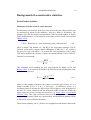
Background of second-order statistics
Second order statistics
Definition of the bivariate K- and L-functions
For stationary and isotropic point processes all second order characteristics can
be expressed by means of the intensity λ and K(r), Ripley’s K function. The
quantity λK(r) has the intuitive interpretation of the expected number of further
points within distance r of an arbitrary point of the process which is not counted
(Ripley 1981):
λ K(r) = E[#(points ≤ r from an arbitrary point of the pattern)]
(A1)
where # means “the number of”, and E[] is the expectation operator. The Kfunction yields under compete spatial randomness (CSR) K(r) = πr2, which is
the area of a circle with radius r. To remove the scale dependence of K(r) under
CSR and to stabilize the variance, a square root transformation of K(r), called Lfunction is used instead:
L (r ) = (
K (r )
− r)
π
(A2)
The commonly used estimator for K(r) was proposed by Ripley (1976) and
Ripley (1981). It is based on all distances dij between the ith and jth point of the
pattern and is given by:
A n n I (d )
Kˆ (r ) = 2 ∑∑ r ij
n i =1 j =1 wij
(A3)
where n is the number of points of the pattern in a study region of area A, Ir is a
counter variable [Ir(dij) =1 if dij ≤ r, and Ir(dij) = 0 otherwise], and wij is a
weighting factor to account for edge effects. The weight wij is the proportion of
the area of a circle centred at the ith point with radius dij that lies within the
study region (for reviews on edge correction see e.g., Haase 1995, or Goreaud &
Pélissier 1999). This edge correction is based on the assumption that the region
surrounding the study region has a point density and distribution pattern similar
to the nearby areas within the boundary.
The bivariate quantity λ2K12(r) follows in a straight-forward manner and has the
20
SUPPLEMENTARY USER MANUAL FOR PROGRAMITA
intuitive interpretation of the expected number of type 2 points within distance r
of an arbitrary type 1 point.
Definition of the g-function and of the O-ring statistic
The pair-correlation function g(r) (Stoyan & Stoyan 1994) is related to the Kfunction by
g (r ) =
1 dK (r )
.
2π r dr
(A4)
Stoyan and Penttinen (2000) provide a heuristic definition: g(r) is related to the
probability p(r) that each of two infinitesimally small discs dx and dy (which are
a distance r away) contain a point of the process:
p(r) = λ2g(r)dxdy
(A5)
Rearrangement of equation A4 and dK(r) = K(r+dr) - K(r) yields
λg(r) = λ [K(r+dr) - K(r)] /(2πr dr)
(A6)
where 2πr dr is the area of a ring with radius r and infinitesimal width dr. Thus,
for isotropic patterns the quantity λK(r) - λK(r+dr) = 2πdr λg(r) may be interpreted, in analogy to equation A1, as the expected number of points in a ring
with radius r and width dr centred at an arbitrary point of the process:
λ g(r) 2πrdr = E[#(r < points < r + dr from an arbitrary point of the pattern)] (A7)
where # means “the number of”, and E[] is the expectation operator. The O-ring
statistic
O(r) = λg(r)
(A8)
is thus the conditional intensity of points at distance r from an arbitrary point of
the pattern.
For a homogeneous Poisson process (= CSR) g(r) = 1. Values g(r) > 1 indicate
that interpoint distances around r are relatively more frequent than they would
be under CSR. If this is the case for small values of r, typically there is clustering. Conversely, values g(r) < 1 indicate that interpoint distances around r are
relatively less frequent than they would be under CSR. If this is the case for
small values of r, the pattern shows regularity.
THORSTEN WIEGAND
21
Grid-based estimators of second-order statistics
The study area is divided into a grid of cells. The size of the cells should be defined as the minimal resolution necessary to respond to the scientific question to
be answered and is limited by the measurement uncertainty of point coordinates
(Wiegand & Moloney 2004). The calculation of point-to-point distances necessary for estimation of second-order statistics is then based on distances between
cells, and counting cells and points in cells.
Grid-based estimator of K- and L-function
Wiegand & Moloney (2004) proposed a simple grid-based estimator of the
bivariate K-function for arbitrarily shaped study regions, which is based on the
mean number of type 2 points found in (complete or incomplete) circles of radius r around all type 1 points k [= P12(r)], divided by the area of these circles
[= A(r)]:
1 n1
∑ Points 2[C1,k (r )]
2 P12 ( r )
2 n1 k =1
ˆ
λ2 K12 (r ) = πr
= πr
1 n1
A(r )
∑ Area[C1,k (r )]
n1 k =1
(A9)
where λ2 = n2/A is the intensity of pattern 2, ni is the number of type i points (i =
1, 2) in the study region, C1,k(r) is the circle with radius r centred on the kth type
1 point, the operator. Points2[X] counts the points of the pattern 2 in a region X
of area A, and the operator Area[X] determines the total number of cells of the
region X.
The circles are incomplete if the focal point has a distance smaller than r to the
border of the study region. Note that this estimator does not scale the number of
points in incomplete circles to the expected number within complete circles as is
commonly done in point pattern analysis (for reviews on edge correction see
e.g., Haase 1995, or Goreaud & Pélissier 1999). The grid-based estimator is
therefore not affected by the problem that the weights may become unbounded
if r becomes larger.
The grid-based estimator of the L-function using equations A2 and A9 yields:
A P12 (r )
λ Kˆ
Lˆ12 (r ) = r ( 2 212 − 1) = r (
− 1) .
n2 A1 (r )
πr
(A10)
22
SUPPLEMENTARY USER MANUAL FOR PROGRAMITA
Grid-based estimator of g- and O-function
An analogous grid-based estimator of the bivariate pair-correlation function
g12(r) is given by
1 n1
Points 2 [ R1w, k (r )]
∑
n
λ2 gˆ12 (r ) = 1 k =1n1
(A11)
1
w
∑ Area[ R1, k (r )]
n1 k =1
where Rw1,k(r) is the ring with radius r and width w centred on the kth type 1
point (Wiegand & Moloney 2004). For the univariate case, this estimator was
e.g., used in Condit et al. (2000).
Selection of ring width
The estimator equation (A11) involves a technical decision on the width w of
the rings. The use of rings that are too narrow will produce jagged plots, as not
enough points will fall into the different distance classes. On the other hand, if
the rings are too wide, the pair-correlation function will lose the advantage that
it can isolate specific distance classes. More sophisticated estimators of the paircorrelation function use kernel functions such as the Epanečnikow kernel with a
bandwidth h instead of rings with width w (see Stoyan & Stoyan (1994) and
references therein).
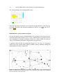
Figure A2. Numerical implementation of the L- function and the O-ring statistic for an irregularly shaped study region. Points of pattern 2 are represented by closed circles, the focal point i
of pattern 1 as open circle within the red cell. Note that we approximate circles and rings with
the underlying grid structure. Study region: grey and white cells, area outside the study region:
black cells. (Left): For numerical implementation of Ripley’s bivariate L-function we count the
number of points of pattern 2 inside the part of the circles around point i of pattern 1 which falls
inside the study region (i.e., the gray shaded area), and the number of cells within this area.
(Right): For implementation of the bivariate O-function we count the number of points of pattern 2 inside the part of the ring around point i of pattern 1 which falls inside the study region
(i.e., the gray shaded area), and the number of cells within this area.
THORSTEN WIEGAND
23
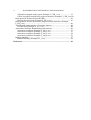
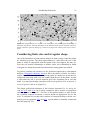
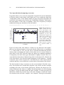
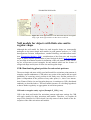
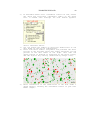
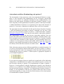
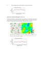
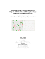
Figure F1. Categorical map of a 27.4m × 13m study plot in the semiarid grass-shrub steppe in
Patagonia (Argentinia), showing individuals of the dominant shrub species Adesmia campestris
(black), Mulinum spinosum (dark grey), and Senecio filaginoides (white). Each cell is 10cm ×
10cm.
Considering finite size and irregular shape
One of the limitations of point pattern analysis in plant ecology is that the plants
are idealized as points. The point approximation is valid where the size of the
plants is small in comparison with the spatial scales investigated, but may obscure the real spatial relationships at smaller scales, the relationship in which
ecologists are mostly interested when interactions among plants are studied.
Programita contains an extension of the grid-based approach to point-pattern
analysis (Wiegand & Moloney 2004) to deal with objects of finite size and irregular shape. The basic idea is to represent plants in a study area by means of a
categorical raster map with a cell size smaller than the size of the plants. A plant
is represented by one or several adjacent grid cells, depending on its size and
shape, in a map representing categories such as bare ground, cover of species 1,
cover of species 2 and so on (figure F1).
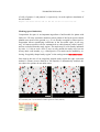
The simple grid-based estimators of the bivariate functions K12, L12 and g12(r)
(eqn A9, A10, and A11) can be easily extended to allow analysis of categorical
raster maps such as Figure F1. The size of the smallest plants, or other criteria
for a minimal required resolution, is used to define an appropriate size for the
cells. To calculate the second-order statistics of categorical maps with the estimators given in equations A10, and A11, a point pattern is formally constructed
from the map (Fig. F2):
24
SUPPLEMENTARY USER MANUAL FOR PROGRAMITA
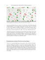
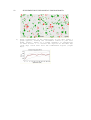
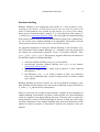
Figure F2. Left: categorical map with a bivariate pattern (red: shrubs of species 1, green: shrubs
of species 2). Right: Point pattern formally constructed from the categorical map shown on the
left. Note that the grid lines indicate 5 × 5 blocks of cells and not the cell size.
A given cell obtains one type 1 point if it is covered by one of the categories
assigned to pattern 1 (e.g. all shrub species) and one type 2 point if it is covered
by one of the categories assigned to pattern 2 (e.g. all grass species), but is
classed as empty if it is not covered by either pattern 1 or 2 but is located within
the study area, and is assigned to the “mask” if the cell is outside the study area.
Although this approach corresponds with conventional point pattern analysis, the
explicit consideration of real world structures (i.e. objects of finite size and irregular shape) prevents an analytical treatment. This extension is therefore a
simulation-based approach for testing specific “ad hoc” hypotheses about the
spatial dependencies of objects in a particular system.
Randomization of objects finite size and real shape
The key for successful application of Programita is the selection of an appropriate null model that responds to the specific biological question asked. The
approach for dealing with objects of finite size and irregular shape allows for
testing specific null models adapted to the biology of the study system and provides a considerable degree of added realism. However, remember that the null
model constitutes a point of reference against which the data are compared.
Therefore the null model must not necessarily describe all particularities of the
real system.
THORSTEN WIEGAND
25
Specific null hypotheses on the considered system can be tested through analysis of the spatial pattern of plants with real shape and finite size. For example,
are plants of a given species randomly (but without overlaps) distributed over
the study area, are the spatial patterns of two species independent, or do plants
of species 2 suffer competition (or facilitation) from plants of species 1? In a
later section we present several important benchmark null models to address
these questions.
Although conceptually analogous to the most simple null models in point pattern analysis (i.e., CSR, heterogeneous Poisson, independence, random labelling, and antecedent condition; Wiegand & Moloney 2004), consideration of the
finite size and irregular shape of plants requires specification of more biological
detail. Specifically, we need to introduce rules and options to decide on the
overlap between plants, explain how to construct objects from a categorical
map, how to randomize the position of the objects, and how to take edge effects
into account which may arise if randomized objects partly overlap the limits of
the study region. How this is implemented in Programita is explained in the
following.
Overlap between plants
An important difference between conventional point-pattern analysis and analysis of categorical maps is that points cannot overlap (except where they occupy
exactly the same location), but for randomisation of the position of plants of finite size rules are needed to determine if they are allowed to overlap or not.
Since a category (and not a number of points) is assigned to each cell, overlap of
two plants of the same pattern is not allowed. (However, to avoid that several
small plants may occupy the same grid cell the size of the grid cell may be reduced.)
Depending on the null hypothesis, we may (or may not) allow overlap of plants
of two different patterns. This difference is important for data collection and
mapping, as for the application of null models. For example, allowing overlap of
the two component patterns of a bivariate pattern is relevant for a null model to
approximate, for instance, “third dimension” effects which may occur if smaller
plants such as grass tufts grow inside larger unpalatable shrubs.
After selecting “Matrix” in How are your data organized?, “Data are given as matrix
map” in Select modus of data, and after specifying in the window Give code numbers
26
SUPPLEMENTARY USER MANUAL FOR PROGRAMITA
which code numbers of your data matrix make up pattern 1, pattern 2,
and the mask, apply the check box “Calculate confidence limits”. A window for
selection of the null model appears (Figure N1) appears. The check box “Only
one point per cell” is always enabled in the matrix
mode. To allow overlap of objects of pattern 1
and pattern 2 enable the check box “Only one
point per pattern”.
for pattern
Figure N2 top right shows a randomization of
pattern 2 without overlap to pattern 1 (null model
“Pattern 1 fix, pattern 2 random”), and figure N2
bottom shows randomization of pattern 2 with the
same null model but allowing overlap to pattern
1.
Figure N1. Window for selection
of null model
Figure N2. Rules for overlap between objects
in null models. Top left: data pattern without
overlap (pattern 1: red, pattern 2: green). Top
right: randomization of objects of pattern 2
(Null model “Pattern 1 fix, pattern 2 random”) without overlap to objects of pattern 1.
Bottom right: randomization of objects of
pattern 2 with overlap to objects of pattern 1.
Overlap is indicated by orange color. Note
that only a few objects overlap.
THORSTEN WIEGAND
27
Construction of objects from categorical map
A categorical map, such as figure N2 top left, contains intuitively discernable
discrete objects; however, in order to randomize the position of these objects for
a given null model Programita must first define objects. This is done with a
percolation algorithm which summarizes all adjacent cells of the same type (i.e.,
type 1 or type 2) as one object.
If pattern 1 of your categorical map comprises objects of finite size and irregular
shape, enable in the window for the selection of the null model (figure N1) the
check box “Pat1”. If pattern 2 of your categorical map comprises objects of finite size and irregular shape, enable additionally check box “Pat2”. After enabling “Pat1” and/or “Pat2”, a small window “Patch determination” opens which
allows you to select specific settings for the definition of the objects.
First, to avoid very large objects, you can define
a maximal size of the objects, given in number
of cells (max patch size pat 1, and max patch
size pat 2). If you e.g., select 100, the algorithm
assigns the first encountered 100 adjacent cells
to a given object, but does consider further adjacent cells as a separate object.
Second, there are three different neighbourhoods used to define adjacency to a
given cell:
• the 4 cell neighbourhood includes only the four immediate (north, east,
south, west) neighbours,
• the 8 cell neighbourhood includes the eight immediate neighbours including the four diagonal neighbours,
• the 12 cell neighbourhood includes the eight immediate neighbours and
additionally the four next (north, east, south, west) neighbours.
The 4 and 8 cell neighbourhood assigns only cells which touch directly to objects, whereas the 12 cell neighbourhood allows you to have objects with small
gaps.
.
28
SUPPLEMENTARY USER MANUAL FOR PROGRAMITA
Separation of joined objects
In some cases discrete objects of a given pattern may touch each other. In this
case the automatic algorithm implemented in Programita will join the two objects to one single object.
One possibility to avoid this problem is to create a
new category for touching objects and to enable
the check box “Use category for defining objects”.
In this case Programita will base the definition of
the objects not only on cells occupied by pattern 1
(or pattern 2), but additionally on the category of
the cells in your original map. In this case an object can only comprise cells of the same category.
Another simple possibility to avoid the problem of joined objects is dividing the
cells into 4 smaller cells and leaving empty cells between adjacent but distinct
objects. Finally, you may manually separate objects.
Manual separation of joined objects
To manually separate objects run first one analysis where adjacent but separate
objects may be joined by Programita. Use the temporal files temppatch1.dat
and temppatch2.dat which are automatically created by Programita and change
the name of temppatch1.dat to name.pa1 and temppatch2.dat to name.pa2 (for
name use an appropriate name). The subfix *.pa1 and *.pa2 are reserved for
manually modified files containing the information on the objects of pattern 1
and pattern 2, respectively.
These files are the “object” representation of your data of pattern 1 and pattern
2. The first line in the files gives the number of objects of pattern 1 (or pattern
2), the next lines contain the information on the objects (each object is a line)
necessary for randomization of the objects of finite size and irregular shape.
The first two columns are the minimal x- and y- coordinates of the object, the
third column gives the width of the object in x-direction (= xmax - xmin), the
fourth column gives the width of the object in y-direction (= ymax - ymin), the
THORSTEN WIEGAND
29
fifth column the number of cells of the objects, and the following columns give
the pairs of coordinates belonging to the object.
For example, the beginning of the temppatch1.dat may be given by:
1
1
185
2
2
6
1
186
1
187
2
186
2
187
2
185
3
186
This indicates that there is 1 object, and the minimal x- and y-coordinates of the
object are 1 and 185, respectively. The width in x- and y-direction of the object
is 2 cells (xmax= 3, xmin=1; ymax=187, ymin = 185), and the object comprises
six cells (1, 186), (1, 187), (2, 186), (2, 187), (2, 185), and (3, 186). This is the
objects with its coordinates:
__185__186__187_
1⎟
X
X
2⎟ X
X
X
3⎟
X
You can now split this object manually into two objects:
object 1 with coordinates: (1, 186), (1, 187), (2, 187), and
object 2 with coordinates: (2, 186), (2, 185), (3, 186):
__185__186__187_
1⎟
X
X
2⎟
X
3⎟
__185__186__187_
1⎟
2⎟ X
X
3⎟
X
To split them you need to modify the file accordingly:
2
1
186
1
1
3
1
186
1
187
2
187
2
185
1
1
3
2
186
2
185
3
186
i.e., adding one objects (2), changing the minimal x- and y-coordinates, the
width, the number of cells belonging to the object, and the coordinates of the
cells.
To help you with this task, Programita creates two temporal files temppatchNr1.dat and temppatchNr2.dat which are a matrix representation of pattern
1 and pattern 2, respectively, but every object is coded with a number numbered
according to the order in the list of objects given in temppatch1.dat and temppatch2.dat:
The beginning of temppatch1.dat is:
49
5 2 4 6 23 5 4 6 4 6 5 6 3 7 4 7 5 7 3 7 6 5 6 6 2 7 2 8 5 8 3 8 6 8 2 7 7 8 7 6 7 9 5 9 6 9 4 7 8 8 8
17 3 1 1 4 17 3 17 4 18 3 18 4
30
SUPPLEMENTARY USER MANUAL FOR PROGRAMITA
The corresponding part of temppatchNr1.dat is:
1
130
0 0
0 0
0 0
0 0
0 0
0 1
0 1
0 1
0 0
0 0
0 0
0 0
0 0
0 0
0 0
0 0
0 0
0 0
0 0
1
0 0
0 0
0 0
0 0
0 1
1 1
1 1
1 0
0 1
0 0
0 0
0 0
0 0
0 0
0 0
0 0
2 2
2 2
0 0
130
0 0 0
0 0 0
0 0 0
0 0 0
0 1 0
1 0 1
1 1 1
1 1 1
1 1 0
0 0 0
0 0 0
0 0 0
0 0 0
0 0 0
0 0 0
0 0 0
0 0 0
0 0 0
0 0 0
x:
1 2 3 4 5 6 7 8 9 ......
0
0
0
0
0
0
1
1
0
0
0
0
0
0
0
0
0
0
0
0
0
0
0
0
0
0
0
0
0
0
0
0
0
0
0
0
0
0
0
0
0
0
0
0
0
0
0
0
0
0
0
0
0
0
0
0
0
0
0
0
0
0
0
0
0
0
0
0
0
0
0
0
0
0
0
0
0
0
0
0
0
0
0
0
0
0
0
0
0
0
0
0
0
0
0
0
0
0
0
0
0
0
0
0
0
0
0
0
0
0
0
0
0
0
0
0
0
0
0
0
0
0
0
0
0
0
0
0
0
0
0
0
0
0
0
0
0
0
0
0
0
0
0
0
0
0
0
0
0
0
0
0
y
y
y
y
y
y
y
y
y
=1
=2
=3
=4
=5
=6
=7
=8
=9
Note that the matrix counts the x-axis from left to right, and the y-axis from top
to bottom. Therefore, the minimal coordinates of object 1 are (5, 2), and of object 2: (17, 3).
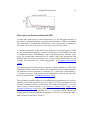
Randomization of the position of objects
Several null models require randomisation of the position of the objects. In conventional point-pattern analysis this is easy: randomisation of points involves
only assignation of random coordinates. However, a plant of finite size may occupy several adjacent cells and its shape needs to be preserved.
Programita achieves this by rotating the objects by 0, 90, 180, or 270 degrees
(each of the four variants being equally probably) and by randomly shifting the
rotated plant as a whole (Figure N3).
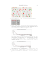
Figure N3. Randomization of position of objects. Left: data pattern, right: randomization of
position of original objects of the data pattern. Arrows indicate for some objects their rotated and
moved counterparts of the null model.
THORSTEN WIEGAND
31
Edge correction if objects fall partly outside the study rectangle
The finite size of the plants requires edge correction since randomly displaced
plants may fall partly outside the arbitrarily selected study rectangle. This would
reduce in the null model the proportion λ of occupied cells and produces a (positive) bias towards aggregation. Programita includes three methods to mitigate
this effect (figure N4).
Plants are not allowed to fall outside.⎯ Randomized plants are not allowed to fall partly outside the study rectangle. This produces a negative
bias towards regularity since fewer plants of the
null model are distributed close to the border.
Thus, the intensity of cells simulated by the null
model is smaller at the border and larger in the
inner parts of the plot (Figure N5).
Figure N4. Option window for
edge correction applied for
randomization of position of
objects
Toroidal correction.⎯ The second method avoids the negative bias produced
by the first method by treating the rectangular study plot encompassing the study
region as a torus, i.e., the part of a plant outside the rectangle is made to appear
at the corresponding opposite border. However, breaking relatively large plants
into two smaller plants produces a slight positive bias.
Smaller study area.⎯ A third method uses the torus correction, but calculates
the second-order statistics only inside an inner rectangle excluding cells close to
the border (guard area). You can select the wide of the guard area (figure N4).
For a guard area wider than the diameter of the largest plants the biases of the
first and the second method disappear, but this may reduce the size of the study
rectangle considerably. Therefore, the guard area may be selected wider than the
diameter of most plants, but still small enough to yield a large enough study rectangle.
To randomise the plants of a given pattern under the above rules, Programita
performs repeated trials for each individual plant. If the provisionally distributed
plant (which was randomly mirrored and shifted) overlaps with an already distributed plant of the same pattern (or the other pattern if appropriate) or falls
partly outside an irregularly shaped study area this trial is rejected. The procedure is repeated until a location is found where both rules are met.
32
SUPPLEMENTARY USER MANUAL FOR PROGRAMITA
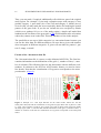
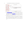
Test of possible bias through edge correction
Programita allows you to assess the magnitude of possible bias in the distribution
of objects relative to the border of the study area. If you enable the check box
“Output data on bias” in the Option window for edge correction (FigureN4), the
results file will contain at the end the line “DistDistanceToBorder” which gives
the total number of cells with x-coordinate x that were occupied by an object
randomized during any simulation of the null model:
DistDistanceToBorder 0,1,2...
0
63 139 203 268 301 310 322 330 369 403 416 ...
450
Number of cells distributed
400
350
300
250
200
Method 1
Method 2
150
Mean
100
Inner mean
50
0
1
21
41
61
81
x-coordinate
101
121
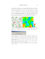
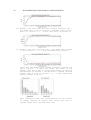
Figure N5. Distribution of
objects of finite size relative to the borders of the
study area. Shown is the
total number of cells in 99
simulations (of the null
model shown in figure N3)
which were occupied by a
cell of pattern 1. Filled
circles: method “Plants are
not allowed to fall outside”,
open circles: method “Toroidal correction”. Horizontal: expected number of
cells.
Figure N5 shows that with method 1 “Plants are not allowed to fall outside”
there are less objects of pattern 1 close to the border (filled circles, x-coordinates
1, 2, 3, and 4, and 127, 128, 129, and 130) as expected (horizontal line) because
objects partly overlapping the border of the study area are rejected. However,
more than 4 cells away from the border the objects are randomly distributed.
Consequently, the inner mean (gray horizontal) is slightly elevated. This is because hardly an object has a diameter larger than 4 cells (figure N3). The bias for
cells closer than 4 cells from the border disappears for the method 2 “Toroidal
correction” (open circles in figure N5). Note that the size of the objects and the
condition that they are not allowed to overlap leads to fluctuations in the density.
The third method of edge correction uses the second method (Toroidal correction), but measures the second-order properties only inside an inner rectangle
excluding cells close to the border (guard area). Because the objects are randomly distributed, this leads to a slightly fluctuating number of cells belonging
to pattern 1 of the null model inside the inner rectangle. To check the degree of
fluctuation (which may become large if the inner rectangle is small) the results
file contains at the end a line “Anzpat1” and “Anzpat2” which gives the number
THORSTEN WIEGAND
33
of cells of pattern 1 and pattern 2, respectively, in each replicate simulation of
the null model:
Anzpat1= 364 350 427 406 407 342 371 349 362 375 383 373 374 376 397 378
Masking (space limitation)
Competition for space is an important ingredient of null models for plants with
finite size. We may encounter situations where plants of the focal species cannot
inhabit some areas of the ground, e.g., if it is already occupied by other species.
Programita allows considering restrictions in the accessible space in an easy
way. All non-accessible cells are summarized as a third pattern (called “mask”)
and are excluded from the study region. The mask may be cells already indicated
by code -1 (*.dat) or code -9999 (*.asc) as cells outside the study area, but can
be any other code number, e.g., a third species. The mask can be enabled by selecting “Irregularly shaped study region” in the settings menu Give modus of analysis.
Note that in the case of an irregularly shaped study region the edge correction
method 1 (Plants are not allowed to fall outside) is automatically enabled; the
two other two options do not make sense.
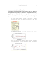
Figure N6 Masking. Data file m_ter_22.dat. Two strips in the left and in the bottom of the plot
are excluded (code 11) and shrubs of other species as well (code 22).
34
SUPPLEMENTARY USER MANUAL FOR PROGRAMITA
Circle approximation
Programita offers an option to analyze the effect of the irregular shape by approximating objects with irregular shape by circular objects of the same size. To
this end enable the check box “Circle” in the window for specifying the null
model below the real shape check boxes.
Figure N7. Circle approximation. Left: data with objects of irregular
shape, right: null model with approximation of objects by circle of
same size. Note that the circles are sometimes not perfectly circular because they have to be approximated by the underlying grid.
Point approximation
Programita offers an option to compare the analysis with objects of finite size
and irregular shape to the common point approximation. Programita approximates the objects by a point with coordinates being the average x- and y- coordinates of the cells belonging to the object.
To this end enable the check box “Point” in the window for specifying the null
model below the real shape check boxes.
THORSTEN WIEGAND
35
Figure N7. Point approximation. Left: data with objects of irregular
shape, right: Point approximation of data shown on the left.
Null models for objects with finite size and irregular shape
Although the null model for finite size and irregular shape are conceptually
analogous to the most simple null models in point pattern analysis (i.e., CSR,
heterogeneous Poisson, independence, random labelling, and antecedent condition; Wiegand & Moloney 2004), consideration of the finite size and irregular
shape of plants requires specification of more biological detail. In the last section
we provided all technical details for definition of the null models, in the following we will present several examples for null models which use the feature of
categorical maps and objects of finite size and irregular shape.
CSR: Randomising plant position for univariate patterns
The most simple and most widely used null model for univariate point patterns is
complete spatial randomness (CSR) where any point of the pattern has an equal
probability of occurring at any position in the study area, and the position of a
point is independent of the position of any other point (i.e., there is no interaction). Plants of finite size and irregular shape are, in analogue to CSR, distributed
randomly as described above. This null model operates as a dividing hypothesis
to detect further regularity or aggregation in univariate patterns.
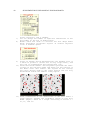
CSR and rectangular study region (Example F_CSR_1.res)
CSR is the basic null model for univariate patterns and most settings for CSR
will apply equally for other univariate null models. Therefore, we explain all
steps of the analysis for CSR in detail, but skip some of these details in the description of the other univariate null models.
36
SUPPLEMENTARY USER MANUAL FOR PROGRAMITA
_________________________________________________________________
Input data file: Figure2.asc
How are your data organized: Matrix
Give modus of analysis Analyze all data in rectangle
Which method will you use? Ring (or Circle)
Ring width: 1 (if intensity λ of cells is too low, select larger ring widths)
Set maximal radius rmax: 30 (too large scales slow down Programita)
Select modus of data: Data are given as matrix map
Give code numbers for pattern: Pattern 1:12 12 12 12 (shrub species Mulinum spinosum)
Pattern 2: 33 33 33 33 (code does not occur)
______________________________________________________________________________
_
1)
highlight the data file "Figure2.asc" in the window Input
2)
3)
4)
select "Matrix" in How are your data organized
select "Analyze all data in rectangle" in Give modus of analysis
select the code numbers for pattern 1 and pattern 2 in Give
code numbers for patterns: write 12 in all windows reserved for
pattern 1 (the species Mulinum spinosum) and write 33 in
all windows reserved for pattern 2 (the code 33 does not
occur in Figure2.asc, therefore you define a univariate
pattern).
5)
data file
select "Ring (Wiegand-Moloney)" in Which method will you use? if
you like to use the O-ring statistic [and Circle (Ripley)
if you like to use the L-function]
6) select an appropriate ring width dr in the box ring width.
Usually a ring width of one cell is appropriate, however,
if the intensity λ of points in the study region is too
low, the graph of the O-ring statistic will be jagged and
selection of a larger ring width dr is appropriate
7) click the button "change" in set maximal radius rmax to define
the maximal scale r of the analysis and insert "30". A too
large scale rmax will slow down Programita.
8) select "Data are given as matrix map" in Select modus of data
9) Click button "Calculate index". Your pattern appears on
the left, and the O-ring function of your data appears on
the right.
10) To determine Monte Carlo confidence limits for CSR, enable
the check box "Calculate confidence limit" on the upper
left. A window with settings for null models appears. Select "Pattern 1 and 2 random":
THORSTEN WIEGAND
37
11) You can change the number of replicate simulations of the
null model in the box "# simulations". If you want to use
the 5th lowest and highest values of 99 (or 999) Monte
Carlos simulations as confidence limits enable the check
box “99” or “999”.
12) Enable check box “Pat1” to activate the real shape modus
where Programita recognizes objects of several adjacent
cells. Two windows open, ”Patch determination” appear on the
left over the map and ”Options for edge correction” right of the
window for specification of the null model:
13) Select in window “Patch determination” the maximal size of
a shrub of pattern 1 (select 400 as very large value), and
the type of neighborhood and confirm with “ok”.
14) Select in the window “options for edge correction” the
rules for randomization of the objects.
15) Press "Calculate index". Now Programita performs the simulations of the CSR null model and shows you the pattern of
the Monte Carlo null models. After termination of the
simulations of the null model a graph appears, showing the
O-ring function of your data (left) and the confidence
limits of your null model (right):
38
SUPPLEMENTARY USER MANUAL FOR PROGRAMITA
16) To save the results of the analysis, press the button
"Save results", which appears below the graph with the results of the univariate analysis, and insert a name for
the result-file. The results-file will be saved as ASCIIfile with a *.res extension in the same directory where
programita.exe is located. It contains the settings of
your analysis and the results of the univariate (and the
bivariate) point-pattern analysis.
17) Programita uses as default the lowest and highest O(r) of
the different simulations of the null model as confidence
limits. However, it automatically produces two temporally
files (Uni_confidence.env, Bi_confidence.env) that contain
the O(r) for all simulations of the null model. The columns of these files are the scales r0 = 1, rmax, and the
lines are the different simulations of the null model. The
temporary files are overwritten if you start a new analysis.
THORSTEN WIEGAND
39
CSR in irregularly shaped study region with mask (Example F_CSR_2.res)
This example shows application of the mask. Competition for space is an important ingredient of null models for plants with finite size. One may encounter
situations where plants of the focal species cannot inhabit some areas of the
ground, e.g., if it is already occupied by other species. Programita facilitates an
elegant extension of the null models CSR and antecedent condition to consider
restrictions in the accessible space. All non-accessible cells are summarized as a
third pattern (called “mask”) and are excluded from the study region.
Masking is especially important for the null model antecedent condition. Not
considering the plants of the third pattern will reduce the intensity of pattern 2,
which then appears to be aggregated in respect to pattern 1. For univariate analysis (i.e., CSR) this effect is only important if larger continuous areas are nonaccessible (e.g., example in Wiegand & Moloney 2004).
_________________________________________________________________
Input data file: m_ter_22.dat
How are your data organized: Matrix
Give modus of analysis Irregularly shaped study region
Which method will you use? Ring (or Circle)
Ring width: 1 (if intensity λ of cells is too low, select larger ring widths)
Set maximal radius rmax: 30 (too large scales slow down Programita)
Select modus of data: Data are given as matrix map
Give code numbers for pattern: Pattern 1: 1 1 1 1 (shrub species 1)
Pattern 2: 2 2 2 2 (code does not occur)
Mask:
22 11 -1 -1 (22: other shrubs, 11: outside strips)
_________________________________________________________________
1)
Highlight the data file "m_ter_22.dat" in the window Input
2)
3)
4)
select "Matrix" in How are your data organized
Enable the check box “Irregularly shaped study region”.
Select the code numbers for pattern 1, pattern 2, and the
mask in Give code numbers for patterns: write 1 in all boxes reserved for pattern 1 (shrub species 1) and write 2 in all
boxes reserved for pattern 2 (the code 2 does not occur in
m_ter_22.dat, therefore you define a univariate pattern),
write in the boxes reserved for the mask 22 (other shrub
species) and 11 (the outside strips):
5)
Click button "Calculate index". Your pattern appears on
the left, and the O-ring function of your data appears on
the right.
To determine Monte Carlo confidence limits for CSR, enable
the check box "Calculate confidence limit" on the upper
left. A window with settings for null models appears:
6)
data file
40
SUPPLEMENTARY USER MANUAL FOR PROGRAMITA
7)
8)
Select "Pattern 1 and 2 random".
You can change the number of replicate simulations of the
null model in the box ”# simulations“.
Enable check box “Pat1” to activate the real shape modus
where Programita recognizes objects of several adjacent
cells. A windows opens:
9)
Select in window “Patch determination” the maximal size of
a shrub of pattern 1 (select 400 as very large value), and
the type of neighborhood and confirm with “ok”.
10) Press "Calculate index". Now Programita performs the simulations of the CSR null model and shows you the pattern of
the Monte Carlo null models. The objects do not overlap
the black “holes” made by the other species and are only
distributed inside the smaller study region.
11) After termination of the simulations of the null model a
graph appears, showing the confidence limits of your null
model (right). There is a slight clustering at scales r =
10, 11, and 12:
THORSTEN WIEGAND
41
Heterogeneous Poisson null model (HP)
If a univariate point pattern is not homogeneous (i.e., the first order intensity of
the pattern is not approximately constant), the null model of CSR is not suitable
for exploration of second-order characteristics, and a null model accounting for
first-order effects has to be used to reveal “true” second-order effects.
A common assumption is that small-scale departures from homogeneity (CSR)
are due to interactions among the points whereas larger-scale departures are due
to exogenous factors. Unfortunately, large-scale heterogeneity critically influences the second-order characteristics at smaller scales and appropriate null
models need to be used to reveal the “true” second order characteristics; see for
example the discussion on “virtual aggregation” in Wiegand and Moloney
(2004).
The heterogeneous Poisson process is the most simple alternative to CSR if the
point pattern shows first-order effects. The constant intensity of the homogeneous Poisson process is replaced by a function λ(x, y) that varies with location (x,
y), but the occurrence of any point remains independent of that of any other (Pélissier & Goreaud 2001; Wiegand & Moloney 2004).
The grid-based approach allows for straightforward generalization of a heterogeneous Poisson null model for objects of finite size if the heterogeneity occurs
for scales well above the size of the plants. The intensity function λ(x, y) is estimated using a kernel estimate (e.g., Bailey & Gatrell 1995; Diggle 2003;
Wiegand & Moloney 2004). Programita includes two different kernel functions
for estimating the intensity function λˆR ( x, y ) : a moving window estimate (the
default) and an estimate using the Epanečnikov kernel. To use the Epanečnikov
kernel enable the check box “kernel”:
42
SUPPLEMENTARY USER MANUAL FOR PROGRAMITA
The first method implemented in Programita uses a moving-window estimate of
the non-constant first-order intensity λ(x, y):
λˆR ( x, y ) =
Points[C( x , y ) ( R)]
(HP1)
Area[C( x , y ) ( R)]
where C(x, y)(R) is a circular moving window with radius R that is centered in cell
(x, y), the operator Points2[X] counts the points of pattern 2 in a region X, and
the operator Area[X] determines the area of the region X. As edge correction,
the number of points in an incomplete circle is divided by the proportion of the
area of the circle that lies within the study region. This is a simple kernel estimate with the kernel function:
⎧1
⎪
eR (d ) = ⎨
⎪0
⎩
0≤d ≤R
(HP2)
d>R
where d is the distance between the focal cell and the counted cell and R the
bandwidth. The second method uses an Epanečnikov kernel recommended by
Stoyan and Stoyan (1994):
⎧3
d2
⎪ 4h (1 − R 2 )
⎪
eh ( R) = ⎨
⎪
0
⎪
⎩
0≤d ≤R
(HP3)
d>R
All points xi surrounding a given location x were counted within distance R, but
weighted with the kernel eR(d), where d is the distance between locations x and
xi. In general, the Epanečnikov kernel produces a smoother intensity function
than the mowing window estimate. An appropriate bandwidth R needs to be larger than the typical size of the plants but smaller than the range over which the
environmental gradient may vary.
For implementation of the heterogeneous Poisson process a given plant is provisionally placed at a random location of the study region, but this plant is only
retained with a probability proportionally to λˆR ( x, y ) , averaged over all cells of
the plant. This procedure is repeated until n points are distributed.
THORSTEN WIEGAND
43
Heterogeneous Poisson (Example F_HP_1.res)
This example applies a heterogeneous Poison null model to the previous example.
_________________________________________________________________
Input data file: m_ter_22.dat
How are your data organized: Matrix
Give modus of analysis Irregularly shaped study region
Which method will you use? Ring (or Circle)
Ring width: 1 (if intensity λ of cells is too low, select larger ring widths)
Set maximal radius rmax: 30 (too large scales slow down Programita)
Select modus of data: Data are given as matrix map
Give code numbers for pattern: Pattern 1: 1 1 1 1 (shrub species 1)
Pattern 2: 2 2 2 2 (code does not occur)
Mask:
22 11 -1 -1 (22: other shrubs, 11: outside strips)
______________________________________________________________________________
1)
2)
3)
4)
Click button "Calculate index". Your pattern appears on
the left, and the O-ring function of your data appears on
the right.
To determine Monte Carlo confidence limits for CSR, enable
the check box "Calculate confidence limit" on the upper
left. A window with settings for null models appears:
Select "Pattern 1 and 2 random".
You can change the number of replicate simulations of the
null model in the box “# simulations“.
Enable check box “Pat1” to activate the real shape modus
where Programita recognizes objects of several adjacent
cells. A windows opens:
44
SUPPLEMENTARY USER MANUAL FOR PROGRAMITA
5)
6)
7)
Select in window “Patch determination” the maximal size of
a shrub of pattern 1 (select 400 as very large value), and
the type of neighborhood and confirm with “ok”.
Enable the check box “Heterogeneous Poisson” in the null
model window. A small settings window for the heterogeneous Poisson process appears:
if you want to use the Epanečnikov kernel enable the check
box “kernel”, insert the radius R = 20 of the moving window (or the bandwidth R if you use the kernel estimator)
and specify which data should be used for construction of
the first-order intensity. Since you have only one pattern
enable “Test only for pattern 1”.
Press "Calculate index". Now Programita calculates the
moving window estimate of the first-order intensity:
On the left the pattern data, on the right the estimated
first-order intensity. The small black gaps are plants of
other species which are excluded from the study area. This
is the intensity estimate using the Epanečnikov kernel
with bandwidth R= 20:
Note that it provides a
somewhat smoother estimate
of the intensity since cells
further away are weighted
lower, but the general pattern does not change. The
bandwidth R has a much larger impact on the intensity
function than the specific
selection of the kernel.
If you want to save the intensity function to use it in
other analyses as plug-in file (see next example) select
OK, otherwise select “Abbrechen”. If you save the file,
the name of the plug-in file will be int_name_R_r.int
THORSTEN WIEGAND
45
where “name” is the name of the data file (here m_ter_22),
and r is the selected value for the radius of the moving
window or bandwidth (here 20).
8)
Programita now performs the simulations of the heterogeneous Poisson null model and shows you the pattern of the
Monte Carlo null model on the right. The objects do not
overlap the black “holes” made by the other species and
are only distributed inside the smaller study region but
more frequently in the pink and red areas of the intensity
map.
9)
After termination of the simulations of the null model a
graph appears, showing the confidence limits of your null
model (right). The slight clustering at scales r = 10, 11,
and 12 visible after applying the CSR null model disappears with the heterogeneous Poisson null model:
46
SUPPLEMENTARY USER MANUAL FOR PROGRAMITA
Heterogeneous Poisson null model: plug-in intensity functions
(Example F_HP_2.res)
The heterogeneous Poisson null model uses the larger-scale intensity of the pattern for construction of the (first-order) intensity function to reveal the smallscale second-order characteristics of the pattern. In some cases, however, you
may have additional information on variables that determine the environmental
heterogeneity, e.g., elevation, or soil type. In this case Programita allows you to
use a plug-in file containing the intensity function.
The plug-in a file has the extension *.int and the following design:
1 150 1 150
1
1 1
1
2 1
1
3 1
15573
1.0000
0.857860
0.799896
0.749270
...
130
130
129 1
130 1
0.074526
0.079002
The first line contains, as usual, the information on the grid size: there are 150
cells in x-direction and 150 cells in y direction, the file contains information on a
total of 15573 cells (if the study area has irregular shape cells outside the study
area do not appear in the list) and the grid size is 1.000 (this information is for
the point modus, in matrix modus it is always 1 since you cannot change the cell
size).
The first column gives the x-coordinate, the second column the y-coordinate, the
third column is always 1, and the fourth column gives the value of the intensity
function at the given cell. Note that the intensity function must be scaled to a
maximum value of 1 and should not have negative values.
Be sure that the dimensions of the study rectangle and of the plug-in file match
exactly!
This example is the same as the previous example, but a plug-in file is used to
provide the intensity. Steps 1 - 5 are the same as in example F_HP_1.res.
_________________________________________________________________
Input data file: m_ter_22.dat
How are your data organized: Matrix
Give modus of analysis Irregularly shaped study region
Which method will you use? Ring (or Circle)
Ring width: 1 (if intensity λ of cells is too low, select larger ring widths)
Set maximal radius rmax: 30 (too large scales slow down Programita)
Select modus of data: Data are given as matrix map
Give code numbers for pattern: Pattern 1: 1 1 1 1 (shrub species 1)
Pattern 2: 2 2 2 2 (code does not occur)
Mask:
22 11 -1 -1 (22: other shrubs, 11: outside strips)
______________________________________________________________________________
THORSTEN WIEGAND
6)
47
Enable the check box “Heterogeneous Poisson” in the null
model window. A small settings window for the heterogeneous Poisson process appears:
to plug-in a file containing the intensity function enable
the check-box “Intensity function from file” and a window
with a list of all *.int plug-in files appears:
7)
Select the file you wand to use (int_m_ter_22_R_20.int).
Since you have only one pattern, enable “pat 1” (the intensity function is used for randomization of pattern 1)
and press “ok”. The intensity function appears on the
right. Click OK in the message window
8)
Press "Calculate index". Programita now performs the simulations of the heterogeneous Poisson null model and shows
you the pattern of the Monte Carlo null model on the
right.
48
SUPPLEMENTARY USER MANUAL FOR PROGRAMITA
Toroidal shift: Independence of bivariate patterns
The null model testing for independence of two point patterns assumes that two
independent stochastic processes created the two component patterns (e.g.,
Goreaud & Pèlissier 2003). Departure from independence indicates that the two
patterns display attraction or repulsion, regardless of the univariate pattern of
either group by itself. Thus, the separate second-order structures of the patterns
in their observed form has to be preserved, the dependence between the two patterns, however, has to be broken (Goreaud & Pèlissier 2003).
This can be achieved by simulations that involve random shifts of the whole of
one component pattern relative to the other. The same idea applies for plants of
finite size and irregular shape: pattern 1 remains fixed whereas pattern 2 is randomly shifted as a whole across the study area, using a torus (toroidal shift).
Note that this null model uses the torus method to treat plants that fall partly outside the study rectangle. For this reason no objects need to be defined and randomized (i.e., you do not need to enable real shape “Pat1” and/or “Pat2”), and
the torus method requires that objects of different patterns are allowed to overlap. The latter may introduce a bias towards repulsion at small scales if the objects are known not to overlap. As an alternative, a univariate null model could
be introduced to describe the second order structure of pattern 2 and, if appropriate, an overlap of plants could be prohibited.
Toroidal shift (Example F_In_1.res)
This example applies a heterogeneous Poison null model to the previous example.
________________________________________________________________
Input data file: m_te22.dat
How are your data organized: Matrix
Give modus of analysis Analyze all data in rectangle
Which method will you use? Ring (or Circle)
Ring width: 1 (if intensity λ of cells is too low, select larger ring widths)
Set maximal radius rmax: 30 (too large scales slow down Programita)
Select modus of data: Data are given as matrix map
Give code numbers for pattern: Pattern 1: 1 1
1 1 (shrub species 1)
Pattern 2: 2 22 22 22 (other shrub species)
______________________________________________________________________________
_
1)
Click button "Calculate index". Your pattern appears on
the left, and the O-ring function of your data appears on
the right.
THORSTEN WIEGAND
2)
3)
4)
5)
49
To determine Monte Carlo confidence limits for CSR, enable
the check box "Calculate confidence limit" on the upper
left. A window with settings for null models appears:
Select "Toroidal shift".
You can change the number of replicate simulations of the
null model in the box "# simulations".
Press "Calculate index". Programita now performs the simulations of the Toroidal shift null model and shows you the
pattern of the null model on the right. Note that the
green pattern is shifted as indicated by the black arrows,
and the objects may overlap (indicated by orange color).
After termination of the simulations of the null model a
graph appears, showing the confidence limits of your null
model (right).
50
SUPPLEMENTARY USER MANUAL FOR PROGRAMITA
Antecedent condition: Randomising only pattern 2
The investigation of some processes, such as investigating facilitation or competition, is less concerned with independence but try to disprove instead that
plants of one pattern are randomly distributed in the neighbourhood of the
plants of the other pattern. Facilitation is indicated if plants of pattern 2 occur
more frequently in the neighbourhood of plants of pattern 1 than expected under
a random distribution of pattern 2 (or expected by the larger-scale intensity of
pattern 2). Conversely, competition is indicated if they occur less frequently.
The appropriate bivariate null model for this question keeps the plants of pattern
1 fixed and distributes the plants of pattern 2 randomly over the area of the
study area not occupied by plants of pattern 1 (called antecedent condition;
Wiegand & Moloney 2004). Note that the null models “antecedent condition”
and “independence” are not the same because “antecedent condition” does not
preserve the observed second-order structure of pattern 2 and thus makes a specific assumption on the second-order structures of pattern 2. If plants of pattern
2 show large-scale variations in their intensity, one may distribute them in accordance to a heterogeneous Poisson null model which keeps the larger-scale
intensity of the pattern (determined as kernel estimate, eq. HP1, HP2, and HP3)
but destroys all second-order structures at smaller scales.
With a bivariate pattern you have different possibilities to randomize pattern 2 if
you select a heterogeneous Poisson null model: you can use pattern 1, pattern 2
or the joined pattern 1 and 2 for construction of the first-order intensity used for
distributing the objects of pattern 2. Which option is appropriate depends on
your biological hypothesis.
If you want to investigate if there are small-scale second-order effects indicating
competition or facilitation between plants of two different species you may use
the first-order intensity of pattern 2 for randomization of plants of pattern 2.
However, if you hypothesis is that the distribution of pattern 2 may depend on
pattern 1 (e.g., if pattern 2 are seedlings and pattern 1 the parent trees) you may
use the first-order intensity of pattern 1 for randomization of plants of pattern 2.
Finally, if your hypothesis is that the two patterns follow the same environmental heterogeneity you may use the first-order intensity of the joined pattern
for randomization of plants of pattern 2.
THORSTEN WIEGAND
51
Antecedent condition (Example F_Ant_1.res)
This example applies a null model under antecedent condition to the previous
example.
________________________________________________________________
Input data file: m_te22.dat
How are your data organized: Matrix
Give modus of analysis Analyze all data in rectangle
Which method will you use? Ring (or Circle)
Ring width: 1 (if intensity λ of cells is too low, select larger ring widths)
Set maximal radius rmax: 30 (too large scales slow down Programita)
Select modus of data: Data are given as matrix map
Give code numbers for pattern: Pattern 1: 1 1 1 1 (shrub species 1)
Pattern 2: 22 2 2 2 (other shrub species)
______________________________________________________________________________
_
1)
2)
3)
4)
Click button "Calculate index". Your pattern appears on
the left, and the O-ring function of your data appears on
the right.
To determine Monte Carlo confidence limits for CSR, enable
the check box "Calculate confidence limit" on the upper
left. A window with settings for null models appears:
Select "Pattern 1 fix, pattern 2 random".
You can change the number of replicate simulations of the
null model in the box “# simulations“.
Press "Calculate index". Programita now performs the simulations of the null model and shows you the pattern of the
null model on the right. Note that only the green pattern
(= pattern 2) is randomized whereas the red pattern (=
pattern 1) does not change:
52
SUPPLEMENTARY USER MANUAL FOR PROGRAMITA
5)
After termination of the simulations of the null model a
graph appears, showing the confidence limits of your null
model (right). There is a slight tendency to aggregation
at small scales r = 1-3:since the objects in the data map
(left map) touch more that the randomized objects (right
map):
THORSTEN WIEGAND
53
Antecedent condition (Example F_Ant_2.res)
This example repeats analysis of the previous example F_Ant_1.res, but allows
overlap between objects of pattern 1 and pattern 2. Comparison between examples F_Ant_1.res and F_Ant_2.res demonstrates the difference such “small”
difference in settings of the null model can make. Therefore you must carefully
select the null model in accordance to the scientific question and knowledge on
hand.
To allow overlap between pattern 1 and pattern 2 enable
the check box “Only one point per pattern” in the null
model window:
The departure from the null model observed in the previous example disappears:
Here for comparison the results without overlap. Note the
stark differences in the confidence limits at smaller
scales r < 10:
54
SUPPLEMENTARY USER MANUAL FOR PROGRAMITA
Antecedent condition (Example F_Ant_3.res)
This example applies a null model with antecedent condition to example
F_Ant_1.res, but uses a heterogeneous Poisson null model for distribution of
pattern 2 instead of CSR.
________________________________________________________________
Input data file: m_te22.dat
How are your data organized: Matrix
Give modus of analysis Analyze all data in rectangle
Which method will you use? Ring (or Circle)
Ring width: 1 (if intensity λ of cells is too low, select larger ring widths)
Set maximal radius rmax: 30 (too large scales slow down Programita)
Select modus of data: Data are given as matrix map
Give code numbers for pattern: Pattern 1:
1 1 1 1 (shrub species 1)
Pattern 2: 22 2 2 2 (other shrubs)
_____________________________________________________________________________
_
1)
2)
3)
Click button "Calculate index". Your pattern appears on
the left, and the O-ring function of your data appears on
the right.
To determine Monte Carlo confidence limits for CSR, enable the check box "Calculate confidence limit" on the
upper left. A window with settings for null models appears:
Select "Pattern 1 fix, pattern 2 random" and enable the
check box “Pat 2” to consider objects of finite size and
irregular shape for pattern 2. You do not need to enable
“Pat 1” since pattern 1 is unchanged in this null model
and does therefore not require definition of objects.
Enable the check box “Heterogeneous Poisson” in the null
model window. A small settings window for the heterogeneous Poisson process appears:
THORSTEN WIEGAND
4)
55
insert the radius R of the moving window (=20) and specify which data should be used for construction of the
first-order intensity. With a bivariate pattern you have
different possibilities: You can use pattern 1 (“Test
only for pattern 1”), pattern 2 (“Test only for pattern
2”) or pattern 1 and 2 (“Test for joined pattern 1 and
2”) for construction of the first-order intensity used
for distributing the objects of pattern 2. Which option
is most appropriate depends on your biological hypothesis. In this example select “Test only for pattern 2”.
Press "Calculate index". Now Programita calculates the
moving window estimate of the first-order intensity:
On the left Programita shows the pattern data, on the
right the estimated first-order intensity. The blue holes
are cells occupied by pattern 1. A message window appears:
5)
6)
7)
If you want to save the intensity function to use it in
other analyses as plug-in file select OK, otherwise select “Abbrechen”. If you save the file, the name of the
plug-in file will be int_name_R_r.int where “name” is the
name of the data file (here m_ter_22), and r is the selected value for the radius of the moving window or bandwidth (here 20).
Programita now performs the simulations of the heterogeneous Poisson null model and shows you the pattern of the
Monte Carlo null model on the right.
After termination of the simulations of the null model a
graph appears, showing the confidence limits of your null
model (right).
56
SUPPLEMENTARY USER MANUAL FOR PROGRAMITA
Antecedent condition (Example F_Ant_4.res)
To show the influence of the selection of the pattern for definition of the first
order intensity we repeat the previous example (F_Ant_3.res), but use the data
of pattern 1 and pattern 2 for construction if the first-order intensity.
Compare the difference of the first-order intensity to
the previous example! However, since both pattern 1 and
pattern 2 follow CSR, there is no difference in the result to the previous example:
THORSTEN WIEGAND
57
Random labelling
Random labelling is the appropriate null model for a null hypothesis corresponding to the absence of interaction between the two types of points if the
points of both patterns were created by one process (e.g., trees), but a subsequent process created the labels “pattern 1” (= surviving trees) and “pattern 2”
(= dead trees) (Goreaud & Pèlissier 2003). The null model of random labelling
then assumes that the process which assigned label to plants was a random process. In a wider sense, random labelling is an appropriate null model to test the
null hypothesis that the labels do not show any spatial structure.
An important ingredient of testing for random labelling is the invariance of gand K-functions under random thinning (i.e., randomly removing points does
not change the second-order properties of uni- or bivariate patterns). Thus,
g11(r) = g22(r) = g12(r) = g21(r). This property suggests different test statistics to
test different aspects of random labelling:
•
•
•
•
univariate random labeling uses g11(r) as test statistic,
conventional bivariate random labeling uses g12(r) as test statistic
(Goreaud & Pèlissier 2003),
the differences g22(r) - g11(r) which tests if pattern 2 is more clustered
than pattern 1,
the difference g12(r) - g11(r) which evaluates if there are (relatively)
more type 2 points than type 1 points in rings (circles) of radius r around
type 1 points.
Random labelling for objects of finite size can be performed in analogy to random labelling of point patterns: here one needs to randomly assign case labels to
n1 of the n1 + n2 objects of the joined pattern.
However, the finite size of objects may introduce violation of the assumption of
random thinning if the number of plants is small and the size class distribution
of the two patterns is not approximately the same. Therefore care is required by
interpreting the results of random labelling for objects of finite size and irregular shape. Departures from random labelling may stem from differences in the
number of objects in pattern 1 and pattern 2 and the size structure of the two
patterns.
58
SUPPLEMENTARY USER MANUAL FOR PROGRAMITA
Random labeling (Example RL_1.res)
In this example we hypothesize that the labels pattern 1 and pattern 2 of objects
of a bivariate pattern are randomly distributed and apply the random labeling
null model. To test the random labeling hypothesis more comprehensibly we use
several test statistics.
________________________________________________________________
Input data file: Figure2.asc
How are your data organized: Matrix
Give modus of analysis Analyze all data in rectangle
Which method will you use? Ring (or Circle)
Ring width: 1 (if intensity λ of cells is too low, select larger ring widths)
Set maximal radius rmax: 30 (too large scales slow down Programita)
Select modus of data: Data are given as matrix map
Give code numbers for pattern: Pattern 1: 13 13 13 13 (shrub species 1)
Pattern 2: 12 12 12 12 (shrub species 2)
_____________________________________________________________________________
1)
2)
3)
4)
5)
highlight the data file "Figure2.asc" in window Input data file.
select "Matrix" in How are your data organized
select "Analyze all data in rectangle" in Give modus of analysis
select "Data are given as matrix map" in Select modus of data
select the code numbers for pattern 1 and pattern 2 in
Give code numbers for patterns: write 12 in all windows reserved
for pattern 1 (the first shrub species) and write 13 in
all windows reserved for pattern 2 (the second shrub species).
6)
enable the check box "Calculate confidence limit" on the
upper left. A window with settings for null models appears. Enable the check boxes “Pat 1” and “Pat 2” and select "Random labeling":
7)
click "Calculate index". Programita now performs the
simulations of the random labeling null model and shows
you the pattern of the null model on the right. Note that
the cells occupied by pattern 1 or pattern 2 are exactly
the same, but the color (= pattern 1 or pattern 2)
changes:
THORSTEN WIEGAND
59
8)
After termination of the simulations a window appears:
9)
Enable first g12 to test for univariate random labeling.
Programita shows the univariate g11-function (instead of
the O-ring statistic) together with the confidence limits
for the univariate random labeling null model:
The results show that the cases (pattern 1) have the same
second-order structure than the joined pattern of case
and control; although there is a non-significant tendency
to be more clustered at scales r < 10. Interestingly, exchanging case and controls (i.e., enabling g21) yields a
different results:
for scales r = 1- 7, pattern 2 is significantly less
clustered than the joined pattern.
10) Using the test statistic g12 - g11 shows that cells of
pattern 2 surround cells of pattern 1 as cells of pattern
1:
60
SUPPLEMENTARY USER MANUAL FOR PROGRAMITA
11) However, the test with the test inverse statistic g21 g22 shows that cells of pattern 1 surround cells of pattern 2 at scales r = 1 - 7 less than cells of pattern 2:
12) Finally, the test statistic g22 - g11 shows that pattern
2 is at scales r = 1 - 7 less clustered than pattern 1:
Since the departures from random labeling occurred for
small scales r < 8 which are within the radius of the
shrubs, they may be due to slight differences in the size
distribution of pattern 1 and pattern 2. Indeed, Mulinum
shrubs (code 12) are at scales r = 1 - 7 (dm) larger than
Senecio shrubs (code 13):
This illustrates that the interpretation of the results
of random labeling of objects with finite site and irregular shape has to be done with care.
THORSTEN WIEGAND
61
References
Bailey, T. C. and Gatrell, A. C. 1995. Interactive spatial data analysis. - Longman Scientific &
Technical
Besag, J. 1977. Contribution to the discussion of Dr. Ripley's paper. - Journal of the Royal Statistical Society B 39: 193-195.
Diggle, P.J. 2003. Statistical analysis of point patterns. Second edition. Arnold, London
Dixon, P. M. 2002. Ripley's K function. - Encyclopedia of Environmetrics 3: 1796-1803.
Goreaud, F. and Pelissier, R. 1999. On explicit formulas of edge effect correction for Ripley's
K- function. - Journal of Vegetation Science 10: 433-438
Goreaud F., and R. Pèlissier. 2004. Avoiding misinterpretation of biotic interactions with the
intertype K12-function: population independence vs. random labeling hypotheses. Journal of
Vegetation Science: 14: 681-692.
Haase, P. 1995. Spatial pattern analysis in ecology based on Ripley's K- function: Introduction
and methods of edge correction. - Journal of Vegetation Science 6: 575-582
Naves, J., T. Wiegand, E. Revilla, and M. Delibes. 2003. Endangered species balancing between natural and human constrains: the case of brown bears (Ursus arctos) in northern
Spain. Conservation Biology 17:1276-1289.
Ripley, B. D. 1981. Spatial statistics. - Wiley
Schadt, S., E. Revilla, T. Wiegand, F. Knauer, P. Kaczensky, U. Breitenmoser, L. Bufka, J.
Cerveny, P. Koubek, T. Huber, C. Stanisa, and L. Trepl 2002. Assessing the suitability of
central European landscapes for the reintroduction of Eurasian lynx. Journal of Applied
Ecology 39:189-203.
Stoyan, D. and Stoyan, H. 1994. Fractals, Random Shapes and Point Fields. Methods of geometrical statistics. - John Wiley & Sons
Upton, G. and Fingleton, B. 1985. Spatial data analysis by example: volume 1: point pattern and
quantitative data. - John Wiley & Sons.
Wiegand T., and K. A. Moloney. 2004 Rings, circles and null-models for point pattern analysis
in ecology. Oikos 104: 209-229.
Wiegand, T., Kissling, W.D., Cipriotti, P.A., and Aguiar, M.R. 2006. Extending point pattern
analysis to objects of finite size and irregular shape. Journal of Ecology