Download Chapter 4 NextOffice Calc

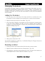
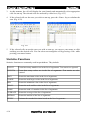
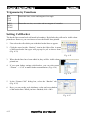
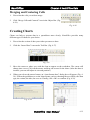
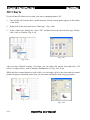
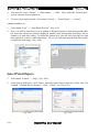
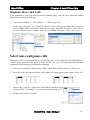
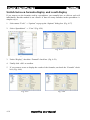
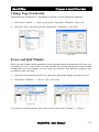
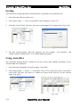
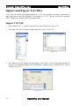
NextOffice
Chapter 4 NextOffice Calc
Chapter 4 NextOffice Calc
Calc is the spreadsheet application of NextOffice, with functions and capabilities comparable to
MS Excel. A spreadsheet usually comprises text, numbers and formulas. You can even make use
of “Function” to perform complicated calculations.
You can also use spreadsheet for managing, sorting, searching and filtering information. Data in
a spreadsheet can be converted into a chart to make the presentation clearer. When changes are
made in the spreadsheet, the changes will automatically be reflected in the chart.
Title bar
Toolbar
Menu
Object
toolbar
Cell
Status bar
Fig. 4-1
A spreadsheet can contain many worksheets and each worksheet may contain many cells
arranged in rows and columns. Each cell can contain a formula, text or numbers.
To directly enter information into a cell, you can double click on it with your mouse.
Alternatively, you can first select your desired cell and then input data into the “Input Line” field
on the top. Confirm your input by pressing the <Enter> key.
When entering information into a cell, you will see the information being displayed in both the
cell and the “Input Line” at the same time (Fig. 4-2). A cell can hold more text than it can show.
If the adjacent cell on its right is blank, its content displayed can be extended to it. However, if
the adjacent cell on the right is not blank, you will see a small red triangle on the right margin of
the cell. This triangle indicates that there is more text in this cell than displayed.
Fig. 4-3
Fig. 4-2
NextOffice User Manual
4-1
NextOffice
Chapter 4 NextOffice Calc
Sometime, the content is longer than it can displayed. In this case, it simply displays marker
“###”. You can widen the cell or set your cell property to “Optimal width” (Select menu
“Format” → “Column” → “Optimal Width”). (Fig. 4-4, 4-5)
Fig. 4-5
Fig. 4-4
Setting up the cells
Auto-fill in Data
When you input sequential data such as months or days of the week, you can make use of sortlists. Instead of filling in every cell, you can quickly drag and fill out the content.
1.
For example, input days of the week. In the first cell, enter the word “Monday”. (Fig. 4-6)
2.
Position the cursor to the bottom right corner of the cell. The cursor will turn into a small
cross.
Fig. 4-7
Fig. 4-6
3.
At this point, hold down the mouse button and drag it down or drag it to the right. The
subsequent sequential data will be listed. You can also drag the mouse up or to the left,
depending on how you wish to arrange the data. (Fig. 4-7)
4.
Release the mouse button when you reach the last cell.
4-2
NextOffice User Manual
NextOffice
Chapter 4 NextOffice Calc
Automatic Line Break in Cell
As mentioned before, if the length of the text is longer than the cell can show, the extra text can
still be displayed if the adjacent cell on the right is blank. However, if the adjacent cell on the
right is not blank, apart from enlarging the cell, you can also display the text by using the
“Automatic Line Break” option.
1.
First select the cell.
2.
Right click on the mouse and select “Format Cells”. (Fig. 4-8)
Fig. 4-8
3.
In the “Format Cell” dialog box, select the “Alignment” tab and check “Automatic Line
Break” check box. Finally, click <OK> to confirm. (Fig. 4-9)
Fig. 4-9
NextOffice User Manual
4-3
NextOffice
Chapter 4 NextOffice Calc
Restricting Input Data Validity
When entering data, you can set the validity of the data. For example, you can set dates as the
only valid data that can appear in column C. This can prevent erroneous data entry.
1.
Select column C.
2.
Select menu “Data” → “Validity”. (Fig. 4-10)
Fig. 4-10
3.
Click on the “Criteria” tab and in the “Allow” field, select “Date”. (Fig. 4-11)
4.
Click on the “Error Alert” tab and check the “show error message when invalid values are
entered” check box. (Fig. 4-12)
Fig. 4-11
5.
4-4
Fig. 4-12
Finally, click <OK>.
NextOffice User Manual
NextOffice
Chapter 4 NextOffice Calc
Managing Row and Column
Managing rows and columns are quite similar. We will use rows as an example. To select the
entire row, for example “Row 1”, click on the row tab marked “1”. (Fig. 4-13)
Fig. 4-13
Changing Row Height
To change the height of a row, position the mouse cursor in between the row tabs. The cursor
will turn to a double-ended arrow and you can then click and drag the mouse cursor up and down
to adjust the height.
Alternatively, you can select the rows, and right click with your mouse on the row tabs and select
“Height” to adjust the height of the rows (Fig. 4-14, 4-15). By choosing “Optimal Row Height”,
Calc will automatically set the optimal row height for you. (Fig. 4-16, 4-17)
Row Height
Fig. 4-15
Fig. 4-14
NextOffice User Manual
4-5
NextOffice
Chapter 4 NextOffice Calc
Optimal Row Height
Fig. 4-17
Fig. 4-16
Insert or Delete Rows
To insert or delete a row, right click on a row tab and select “Insert Rows” (Fig. 4-18) or “Delete
Rows” accordingly. (Fig. 4-19)
Fig. 4-19
Fig. 4-18
Show or Hide Row
To hide or show a row, right click on a row tab and select “Hide” (Fig. 4-20) or “Show”
accordingly. (Fig. 4-21)
Fig. 4-21
Fig. 4-20
4-6
NextOffice User Manual
NextOffice
Chapter 4 NextOffice Calc
Managing Worksheets
A spreadsheet can contain a number of worksheets. On the bottom of the window, you can see
different tabs each identifying a worksheet, marked “Sheet 1”, “Sheet 2”, etc. By default, a new
spreadsheet contains only 3 worksheets. However, you can add or delete worksheets at any time
according to your needs. You can also name each worksheet to clearly show that information
each one contains.
Adding New Worksheet
1.
Move the mouse cursor to the bottom of the window and click on a worksheet tab to select
the worksheet. The new worksheet can be inserted before or after the selected worksheet.
2.
Right click on the mouse and select “Insert Sheet”. (Fig. 4-22)
3.
In the “Insert Sheet” dialog box, select whether you wish to insert the new worksheet before
or after the current worksheet, the name of the new worksheet and the number of
worksheets. If you insert more than 1 worksheet, they will automatically be numbered and
arranged accordingly. (Fig. 4-23)
Fig. 4-22
4.
Fig. 4-23
When you have finished click <OK>.
You can delete worksheets in a similar way. A confirmation dialog box will appear and you can
click “Yes” to confirm the deletion.
Renaming worksheet
1.
Position your mouse cursor on the tab label of the sheet that you want to rename.
2.
Right click on the worksheet tab and select “Rename Sheet”. (Fig. 4-24)
3.
In the dialog box, enter the new name and then click <OK>. The name of the worksheet can
contain English words or Chinese characters or numbers. (Fig. 4-25)
NextOffice User Manual
4-7
NextOffice
Chapter 4 NextOffice Calc
Fig. 4-25
Fig. 4-24
Navigating Worksheets
If you have inserted many worksheets and their tabs cannot all be displayed, the “Tab bar” will
show more navigation options: (Fig. 4-26)
Fig. 4-27
Fig. 4-26
1.
Move to the first or last worksheet.
2.
Move to the preceding or following worksheet.
3.
When the mouse is placed here, the cursor will change into a double-ended arrow and you
then drag the mouse to widen the tab bar to display more worksheet tabs. (Fig. 4-27)
Hide Grid Lines
To not display the grid lines, select menu “Tools” → “Options” → “Spreadsheet” → “View”
(Fig. 4-28), un-check the “Grid lines” check box. (Fig. 4-29)
Fig. 4-29
Fig. 4-28
4-8
NextOffice User Manual
NextOffice
Chapter 4 NextOffice Calc
Formulas and Charts
Basic Formula Symbols
Formulas provide basic functions to the spreadsheet. When setting the formulas, you have to
enter different formula symbols. Following is a concise guideline:
Symbols
Description
Examples
=
Equal
=123 + 456
+
Add
=A1 + 19
-
Subtract
=B3 – C6
*
Multiple
=10*10
/
Divide
=100 / 25
^
Index
=10^2 (10 to the power of 2 )
<
Less than a condition
=if(A1<A2; “too much”, “drop some”)
>
Greater than a condition
=if(A1>A2; “too little”; “add more”)
<=
Less than or equal to a condition
=if(B1<=100; “too little return”; “deal!”)
>=
Greater than or equal to a condition
=if(B1>=300; “too expensive”; “deal!”)
<>
Not equal to a condition
=if(D1<>D2; “no discrepancy”; “balance”)
:
A range of cells
=sum(A1:A9) (summation of cells from A1
to A9)
;
A range of non-contiguous cells
=sum(A1;A3;A5) (summation of cell A1, A3
and A5)
* Note the “=” symbol is very important. All formulas must be preceded by the “=” symbol or
they will consider as a string instead of formulas.
Short cut to Sum function
In the “Formula Bar”, there is a small “Sum” icon which can be used to
quickly add up numbers.
1.
First, click on the cell you wish your sum to appear in.
2.
Then click on the “Sum” icon in the “Formula bar”. (Fig. 4-30)
Fig. 4-30
NextOffice User Manual
4-9
NextOffice
Chapter 4 NextOffice Calc
3.
At this moment, the cell will display the sum formula and automatically select appropriate
cells for sum up. The selected cells are enclosed by a blue box. (Fig. 4-31)
4.
If the selected cells are the ones you wish to sum up, press the <Enter> key to calculate the
sum. (Fig. 4-32)
Fig. 4-31
5.
Fig. 4-32
If the selected cells are not the ones you wish to sum up, you can use your mouse to click
and drag over the desired cells. You can select non-contiguous cell by pressing <Ctrl> while
pressing your mouse button.
Statistics Functions
Statistics functions are commonly used in spreadsheets. They include:
COUNT
Count how many numbers are in the list of arguments. Text entries are ignored.
COUNTA
Count how many values are in the list of arguments. Text entries are also
counted.
MAX
Return the maximum value in the list of arguments.
LARGE
Return the n-th largest value in the list of arguments.
MIN
Return the minimum value in the list of arguments.
SMALL
Return the n-th smallest value in the list of arguments.
RANK
Return the rank of a number in the list of arguments.
AVERAGE
Return the average of the list of arguments.
MEDIAN
Return the median of the list of arguments.
STDEV
Estimate the standard deviation based on the list of arguments.
4-10
NextOffice User Manual
NextOffice
Chapter 4 NextOffice Calc
Date and Time Functions
Date and Time functions are used to manipulate data like: year, month, day, hour, minute, second
and weekdays.
TODAY
Return the current computer system date.
NOW
Return the current computer system date and time.
DAYS
Calculate the difference between 2 date values.
YEAR,
DAY,
MONTH,
HOUR,
MINUTE,
SECOND
Return the value of year, day, month, hour, minute and second respectively.
Today and Now are updated automatically when you re-open or modify the document.
Logic Functions
Using logic functions.
AND
Return true if both TRUE, otherwise return FALSE
OR
Return false if both FALSE, otherwise return TRUE
NOT
Reverse the boolean result
IF
Specify a logic test to be performed based on the boolean result
Mathematical Functions
MOD
Return the remainder after a number is divided by a denominator
ABS
Return the absolute value of a number
INT
Round a decimal number down to the nearest integral value
ROUND
Return a decimal number rounded to a certain number of decimal places
COUNTIF
Return the number of elements that meets with certain criteria within a cell range
SUMIF
Add the cells specified in a given criteria
RAND
Return a random number between 0 and 1
NextOffice User Manual
4-11
Chapter 4 NextOffice Calc
NextOffice
Trigonometry Functions
SIN,
COS,
TAN
Return the sine, cosine and tangent of an angle
ASIN,
ACOS,
ATAN
Return the arc sine, arc cosine and arc tangent of a number
Setting Cell Border
The border lines around each cell mark its boundary. By default, they will not be visible when
printed out. However, you can choose to have the border lines printed.
1.
First select the cells which you wish their border lines to appear.
2.
Click the arrow besides “Borders” icon in the Object Bar. A menu
of different border line types will pop-up for you to choose from.
(Fig. 4-33)
Fig. 4-33
3.
When border lines have been added in, they will be visible when
printed out.
4.
If you want further settings with borders, you can select menu
“Format” → “Cell” to make further customization. (Fig. 4-34)
Fig. 4-34
5.
In the “Format Cells” dialog box, select the “Borders” tab.
(Fig. 4-35)
6.
Here, you can set the style, thickness, color and even shadow
of the border lines. When you have finished, click <OK>.
Fig. 4-35
4-12
NextOffice User Manual
NextOffice
Chapter 4 NextOffice Calc
Merging and Centering Cells
1.
First select the cells you wish to merge.
2.
Click “Merge Cells and Centered” icon in the Object Bar. (Fig.
4-36)
Fig. 4-36
Creating Charts
Charts can help to present data in a spreadsheet more clearly. NextOffice provides many
different types of charts for your choice.
1.
First select the section of data you wish to present as a chart.
2.
Click the “Insert Chart” icon on the Tool Bar. (Fig. 4-37)
Fig. 4-37
3.
Move the cursor to where you wish the chart to appear on the worksheet. The cursor will
change into a cross. Click on the mouse and drag out an area for the chart. (After the chart is
inserted, you can still adjust its size and position.)
4.
When you release the mouse button, an “Auto-format chart” dialog box will appear (Fig. 438). Follow the guidelines to set the chart format, such as choosing the axes labels, the chart
type, the variant, the title, the axes etc. Finally, click <OK> to confirm. (Fig. 4-39)
Fig. 4-38
Fig. 4-39
NextOffice User Manual
4-13
NextOffice
Chapter 4 NextOffice Calc
3D Charts
If you feel that 2D charts are too plain, you can try changing them to 3D.
1.
First, double click on the chart. At this moment, 8 black control points appear on the border
of the chart.
2.
Right click on the chart and select “Chart type”. (Fig. 4-40)
3.
In the “Chart type” dialog box, select “3D” and then choose the desired chart type. Finally,
click <OK> to confirm. (Fig. 4-41)
Fig. 4-41
Fig. 4-40
After you have finished creating a 3D chart, you can right click on the chart and select “3D
effects” to adjust effects, such as shading, illumination, etc. (Fig. 4-42, 4-43)
While the black control points are still visible, you can single click on the chart and red control
points will appear around the chart. Now you can rotate and tilt the chart using your mouse.
Fig. 4-42
Fig. 4-43
4-14
NextOffice User Manual
NextOffice
Chapter 4 NextOffice Calc
Printing in Calc
There are some differences between printing in a spreadsheet and other applications.
Page Header and Footer
1.
Select menu “Format” → “Page” and a “Page Style” dialog box will appear. (Fig. 4-44)
2.
Select the “Header” (or “Footer”) tab and check the “Header on” check box. Then click
“Edit”.
3.
Now, you can select the file name, sheet name, page number, number of pages, date or time
to be displayed on the header (or footer) as well as the font type. (Fig. 4-45)
Fig. 4-45
Fig. 4-44
Setting Print Range
1.
First select the section you wish to print.
2.
Select menu “Format” → “Print Ranges” → “Define”. (Fig. 4-46)
3.
If you have define a print region before and now you want to define more, then select
“Format” → “Print ranges” → “Add”.
Fig. 4-46
NextOffice User Manual
4-15
NextOffice
Chapter 4 NextOffice Calc
4.
You may also select “Format” → “Print Range” → “Edit”. Then, under the “Print Region”
section, enter the desired print area.
5.
To cancel print region section, select menu “Format” → “Print Region” → “Cancel”.
Another method is to:
1.
Select menu “View” → “Page Break Preview”. (Fig. 4-47)
2.
Now, you will see that the areas to be printed is displayed against a white background while
the areas that will not be printed is displayed against a gray background. Each page will be
framed by a dark blue border. To define the printed area, you can first select the area and
then right click to select “Add Print Range”. Or you can click and drag the dark blue border
to adjust the print ranges. (Fig. 4-48)
Fig. 4-47
Fig. 4-48
Select Print Objects
1.
Select menu “Format” → “Page”. (Fig. 4-49)
2.
In the pop-up dialog box, click “Sheet” and select print objects under the “Print” title. For
example, “Column and row headers”, “Grid”, “Charts”, etc. (Fig. 4-50)
Fig. 4-49
4-16
Fig. 4-50
NextOffice User Manual
NextOffice
Chapter 4 NextOffice Calc
Duplicate Rows and Cells
If the spreadsheet is too big and runs across multiple pages, you can set to print out column
labels and row labels on each page.
1.
Select menu “Format” → “Print Ranges” → “Edit”. (Fig. 4-51)
2.
In the “Row to Repeat” or “Column To Repeat” field of the pop-up dialog box, select the
row or column which you want to appear in every page. If the title is in Row 1, enter “$1” as
the row. If the title is in A column, enter “$A” in column. Then press <OK>. (Fig. 4-52)
Fig. 4-52
Fig. 4-51
Select non-contiguous cells
Sometimes we have to format different cells in a same way. If we format each cell individually, it
could be quite inefficient and prone to error. In this case, you can format adjacent and noncontiguous cells collectively by doing the following:
1.
Select a cell you wish to format. Press “Shift” and left click with your mouse. (Fig. 4-53)
2.
Press the <Ctrl> key and left click to select other cells applying the same format. (Fig. 4-54)
Fig. 4-54
Fig. 4-53
3.
Release the <Ctrl> key, right click on the mouse and then select
“Format Cells”. You can now set your desired format. (Fig. 4-55)
4.
Finally, click <OK> to confirm.
Fig. 4-55
NextOffice User Manual
4-17
NextOffice
Chapter 4 NextOffice Calc
Switch between formula display and result display
If you want to see the formulas used in a spreadsheet, you normally have to click on each cell
individually. But this method is not effective if there are many formulas in the spreadsheet. A
simpler way is:
1.
Select menu “Tools” → “Options” to pop-up the “Options” dialog box. (Fig. 4-57)
2.
Select “Spreadsheet” → “View” (Fig. 4-58)
Fig. 4-58
Fig. 4-57
3.
Under “Display”, check the “Formula” check box. (Fig. 4-59)
4.
Finally click <OK> to confirm.
5.
If you want to revert to display the results of the formulas, un-check the “Formula” check
box. (Fig. 4-60)
Fig. 4-59
4-18
Fig. 4-60
NextOffice User Manual
NextOffice
Chapter 4 NextOffice Calc
Change Page Orientation
The default page orientation of a spreadsheet is portrait. It can be changed to landscape:
1.
Select menu “Format” → “Page” to pop-up the “Page Style” dialog box. (Fig. 4-61)
2.
Select the “Page” tab and specify the orientation as “Landscape”. (Fig. 4-62)
Fig. 4-61
Fig. 4-62
Freeze and Split Window
If the rows and columns in the spreadsheet are too long and cannot be displayed in full view, you
can choose to freeze some of the rows and columns. By freezing their position and scrolling
through other rows and columns you can easily cross-reference two different sections in your
spreadsheet at the same time.
1.
Select the cell just underneath the rows and on the right of the columns you wish to freeze.
2.
Select menu “Window” → “Freeze”. (Fig. 4-63, 4-64)
Fig. 4-63
Fig. 4-64
If you want to scroll through the frozen area as well, select menu “Window” → “Freeze”.
NextOffice User Manual
4-19
NextOffice
Chapter 4 NextOffice Calc
Sorting
You can use the sorting functions to sort the data in a spreadsheet in a particular way:
1.
First select the cells you wish to sort.
2.
Select menu “Data” → “Sort” to pop-up the “Sort” dialog box. (Fig. 4-65)
3.
Select the “Sort Criteria” tab. Here, you can set a maximum of 3 sorting criteria. (Fig. 4-66)
Fig. 4-65
Fig. 4-66
4.
For more sorting options, select the “Options” tab. For example, “Case Sensitive” and
“Range contains column labels” are available additional options.
Using Auto-filter
The Auto-filter function inserts a combo box on one or more data columns and allows you to
select the data to be displayed.
1.
First select the column that you wish to apply “Auto-filter”.
2.
Select menu “Data” → “Filter” → “Auto-filter” (Fig. 4-67) or click once in the “Auto-filter”
icon on the Tool Bar. You will see a combo box arrow in the first row of your selected
range. (Fig. 4-68)
Fig. 4-67
Fig. 4-68
4-20
NextOffice User Manual
NextOffice
3.
Chapter 4 NextOffice Calc
Single click on the drop-down arrow in the column heading and select an item. Only those
rows whose contents meet the filter criteria are displayed. The other rows will be hidden.
Using Standard Filtering
For standard filter, you can set a maximum of 3 filtering criteria.
1.
First select the area you wish to use standard filter on. (Fig. 4-69)
2.
Select menu “Data” → “Filter” → “Standard Filter” to bring up the “Standard Filter” dialog
box. (Fig. 4-70)
Fig. 4-70
Fig. 4-69
3.
For example, you may want to filter out from some weather data, such as only temperatures
exceeding 20 degrees, humidities greater than 80%, and months with rainfall exceeding
80mm. You can input these criteria in the relevant fields in the dialog box.
4.
Finally click <OK> to confirm.
You can also copy the filter results into another cell:
Click on “More” button for more filter options. You can check the “Copy results to...” check box
then click on the “Shrink” icon on the far right. The dialog box will shrink and you can select the
cell you wish to copy the results into. Then you can click on the icon on the far right of the
dialog box again to resize its size. Finally click <OK>.
NextOffice User Manual
4-21
NextOffice
Chapter 4 NextOffice Calc
Import and Export Text Files
“CSV” files are text files that contain plain text. “CSV” files usually use commas, semicolons, or
other characters as the field delimiters. Text strings in a “CSV” file are enclosed by quotation
marks, numbers are written without quotation marks.
Import CSV File
1.
Select menu “File” → “Open” to pop-up the “Open” dialog box. (Fig. 4-71)
2.
Select the CSV file you wish to import and click “Open”. (Fig. 4-72)
Fig. 4-72
Fig. 4-71
3.
An “Import Text File” dialog box will appear. Click <OK>. You can select the typeface for
the text to be imported and also the field delimiters. When you have finished, click <OK> to
confirm. (Fig. 4-73)
Fig. 4-73
4-22
NextOffice User Manual
NextOffice
Chapter 4 NextOffice Calc
Export CSV File
1.
Select the spreadsheet you wish to export as a “CSV” file.
2.
Select menu “File” → “Save as” to pop-up the “Save as...” dialog box. (Fig. 4-74)
3.
In the “File type” field, select the format “Text CSV”. Enter the name for the file and click
“Save”. (Fig. 4-75)
Fig. 4-74
Fig. 4-75
4.
An “Export to text files” dialog box will appear. Select the character set, the field and the
text delimiters then click <OK> to confirm. (Fig. 4-76)
Fig. 4-76
Note that if the text uses commas for decimal or thousands separators, do not select the comma as
a delimiter. Or, if the text uses double quotation marks, you must use single quotation marks as a
separator.
NextOffice User Manual
4-23